Singular vortex pairs follow magnetic geodesics

Abstract.

We consider pairs of point vortices having circulations $\Gamma_{1}$ and $\Gamma_{2}$ and confined to a two-dimensional surface $S$. In the limit of zero initial separation $\varepsilon$, we prove that they follow a magnetic geodesic in unison, if properly renormalized. Specifically, the “singular vortex pair” moves as a single charged particle on the surface with a charge of order $1/\varepsilon^{2}$ in a magnetic field $B$ which is everywhere normal to the surface and of strength $|B|=\Gamma_{1}+\Gamma_{2}$. In the case $\Gamma_{1}=-\Gamma_{2}$, this gives another proof of Kimura’s conjecture [11] that singular dipoles follow geodesics.

1. Introduction

One of the most classical areas of hydrodynamics is the study of the motion of point vortices in 2D ideal fluids. In this paper we are describing the limiting motion of a vortex pair on arbitrary surfaces. Let $S$ be a closed surface embedded in $\mathbb{R}^{3}$ with an induced area form $\mu_{S}$. (For most of our considerations one does not need the embedding and can trace the vortex motion on an abstract 2D surface, but we assume it now to simplify the introduction.) Consider a pair of vortices located at $z_{1},z_{2}\in S$ and the singular vorticity form

$$\omega(x)=\Gamma_{1}\delta_{z_{1}(t)}(x)+\Gamma_{2}\delta_{z_{2}(t)}(x)-\frac{\Gamma_{1}+\Gamma_{2}}{{\rm Area}(S)}\,.$$ (1.1)

Here the constant term is understood as a multiple of the area form, $(\Gamma_{1}+\Gamma_{2})\mu_{S}/{\rm Area}(S)$, which ensures that the vorticity form is exact, i.e. it has zero total integral over $S$. (By abusing the notation we omit $\mu_{S}$ below.) Vortex positions evolve in time according to the Kirchoff–Helmholtz equations, see §2. We are interested in the dynamical properties of the vortices as the width of the vortex pair tends to zero:

$$\|z_{1}(0)-z_{2}(0)\|=\varepsilon\to 0\,,$$ (1.2)

where $\|\cdot\|$ is the distance in $\mathbb{R}^{3}$. In the case of a dipole $\Gamma_{1}=-\Gamma_{2}$, Kimura conjectured (and proved for surfaces of constant curvature) that when the width tends to zero the (singular) dipole moves along a geodesic on the surface [11]. As such, Kimura noted that singular vortex dipoles are “curvature checkers”. The general case was proved by Boatto and Koiller [3] using Gaussian geodesic coordinates (see also [9]) and by Gustafsson [10] using complex analytic techniques.

In this paper, we extend this picture to more general vortex pairs with different circulations. We prove that singular vortex pairs evolve as a charged particle confined to $S$ solely under the influence of a magnetic field of constant strength proportional to the sum $\Gamma_{1}+\Gamma_{2}$ and everywhere normal to the surface. As such, general vortex pairs follow magnetic geodesics. Only in the case of the exact dipole $\Gamma_{1}=-\Gamma_{2}$ does the magnetic effect disappear and it follows the ordinary geodesic.

Recall that a curve $X:\mathbb{R}\to S$ parametrized by $t\in\mathbb{R}$ is a magnetic geodesic if it is a solution of the following magnetic geodesic equation:

$$\ddot{X}(t) =\mathrm{I\!I}_{X(t)}(\dot{X}(t),\dot{X}(t))+\mathsf{q}\,\dot{X}(t)\times B(X(t))$$ (1.3)

where $\mathrm{I\!I}_{x}(v,u)$ is the second fundamental form of the surface $S\subset\mathbb{R}^{3}$, a constant $\mathsf{q}$ is the charge, and $B$ is the magnetic vector field, which is everywhere orthogonal to the surface. The geodesic is defined by setting the initial conditions $X(0)$ and $\dot{X}(0)$.

Our main result is the following statement:

Theorem 1.1.

Let $z_{1}^{\varepsilon}(t)$ and $z_{2}^{\varepsilon}(t)$ be two point vortices on $S$ such that $\|z_{1}^{\varepsilon}(0)-z_{2}^{\varepsilon}(0)\|=\varepsilon$. The paths $\{z_{i}^{\varepsilon}(t)\}_{t\in\mathbb{R}}$ have following asymptotics: for any fixed moment $t\in\mathbb{R}$ they tend to the corresponding magnetic geodesic as $\varepsilon\to 0$, provided that renormalizations of $\Gamma_{i}$ enforce

$$\frac{\Gamma_{2}-\Gamma_{1}}{\varepsilon}=O(1)\qquad\text{and}\qquad\frac{\Gamma_{1}+\Gamma_{2}}{\varepsilon^{2}}=O(1)\qquad\text{as}\qquad\varepsilon\to 0.$$ (1.4)

Namely, there is a family of curves $X_{\varepsilon}:\mathbb{R}\to S$ such that for $i=1,2$

$$\|{z}_{i}^{\varepsilon}(t)-X_{\varepsilon}(t)\|\to 0\quad\text{as}\quad\varepsilon\to 0$$

where $X_{\varepsilon}(t)$ solves the magnetic geodesic equation (1.3) for the magnetic field

$$B(x)=({\Gamma_{1}+\Gamma_{2}})\hat{n}_{S}(x),$$ (1.5)

normal to the surface $S$ and the charge $\mathsf{q}=\frac{1}{2\pi\varepsilon^{2}}$. The initial conditions at $t=0$ are

$$X_{\varepsilon}(0)=\mathsf{p},\qquad\dot{X}_{\varepsilon}(0)=\left(\frac{\Gamma_{2}-\Gamma_{1}}{2\varepsilon}\right)\mathsf{w}\times\hat{n}_{S}(\mathsf{p}),$$ (1.6)

where $\mathsf{p}=\lim_{\varepsilon\to 0}\frac{1}{2}(z_{1}^{\varepsilon}(0)+z_{2}^{\varepsilon}(0))$ is the midpoint of the vortex pair and $\mathsf{w}=\lim_{\varepsilon\to 0}\frac{z_{1}^{\varepsilon}(0)-z_{2}^{\varepsilon}(0)}{\|z_{1}^{\varepsilon}(0)-z_{2}^{\varepsilon}(0)\|}$ is the initial unit separation vector.

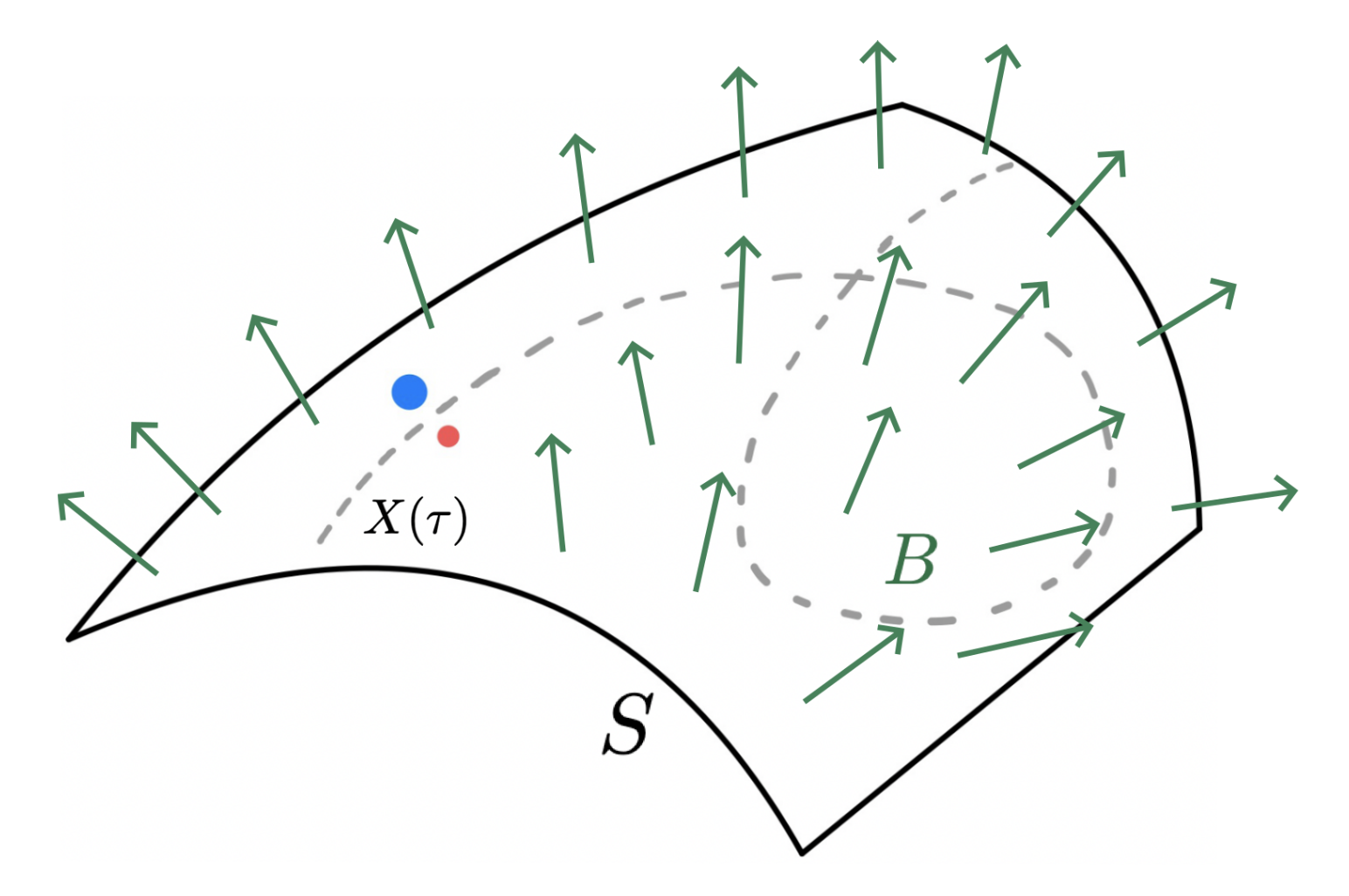
Figure 1. An asymmetric vortex pair follows a magnetic geodesic on a surface.

Corollary 1.2.

For a dipole, $\Gamma_{1}=-\Gamma_{2}$, the magnetic field vanishes and Eqn. (1.3) describes the geodesics on $S$. Thus, in the limit $\varepsilon\to 0$, dipoles move along the geodesics on the surface $S$.

Theorem 1.1 can be understood as follows. Two vortices at a distance of order $\varepsilon$ move each other with the velocity of order $\Gamma/\varepsilon$. So the initial speed of the limiting magnetic geodesic is also of order $\Gamma/\varepsilon$. At the time of order $O(1)$ they could diverge at the distance of order $\Gamma/\varepsilon$. By aligning their initial velocities this distance is made of order $O(1)$. The theorem says that if, in addition, the acceleration satisfies the magnetic geodesic equation, then this distance will be of order $\varepsilon$, i.e. given by the next term in the $\varepsilon$-expansion. In this context, this is equivalent to the statement that the latter distance goes to zero as $\varepsilon\to 0$.

It is interesting to compare this setting with the gyroscope motion described by Cox and Levi [4]. The averaged motion of a gyroscope follows a magnetic geodesic in a magnetic field proportional to the Gaussian curvature of the surface $S$. Here, for the vortex pair, the magnetic field is constant and proportional to the sum of vortex strengths, $\Gamma_{1}+\Gamma_{2}$.

Remark 1.3 (Units).

Note that circulation has units of (vorticity)$\times$(area) = $\mathsf{L}^{2}/\mathsf{T}$. The units of the magnetic field (setting mass $\mathsf{m}=1$) are $1/(\mathsf{T}^{2}\mathsf{Amp})=1/(\mathsf{T}\mathsf{C})$ where $\mathsf{C}$ denotes one unit of charge $\mathsf{q}$. In our “magnetic dictionary” the coulomb charge units translate to the inverse area: $\mathsf{C}\equiv 1/\mathsf{L}^{2}$. The quantity $\mathsf{q}B$ has units $1/\mathsf{T}$.

Remark 1.4 (Scalings).

In order for the initial speed and $\mathsf{q}B$ to be finite as $\varepsilon\to 0$, one requires (1.4). This could be accomplished, for instance, by taking

$$\Gamma_{i}=c_{i}\mathsf{v_{0}}\varepsilon$$ (1.7)

where $\mathsf{v_{0}}$ is fixed with units of velocity and $c_{1}$ and $c_{2}$ are dimensionless functions of $\varepsilon$ satisfying

$$c_{1}=c_{1}(\varepsilon)=\frac{\mathsf{c}}{2}\varepsilon+1,\qquad c_{2}=c_{2}(\varepsilon)=\frac{\mathsf{c}}{2}\varepsilon-1.$$ (1.8)

One should imagine here a limit where circulations are scaled down in proportion to the inter-vortex distance, while simultaneous becoming closer to a vortex dipole at a rate which maintains a finite effect of the Lorentz force.

Example 1.5 (Motion on the plane).

On the plane, two point vortices with circulations $\Gamma_{1}$ and $\Gamma_{2}$ sitting at $z_{1}$ and $z_{2}$ rotate about the center of vorticity located at $z_{c}=(z_{1}\Gamma_{1}+z_{2}\Gamma_{2})/(\Gamma_{1}+\Gamma_{2})$ with angular velocity $\xi=(\Gamma_{1}+\Gamma_{2})/(2\pi\varepsilon^{2})$, where $\varepsilon$ is the pair width $\varepsilon=\|z_{1}-z_{2}\|$, see e.g. [13]. In the magnetic field $B$ the angular velocity of a particle of mass $\mathsf{m}$ and charge $\mathsf{q}$ is $\xi=\mathsf{q}B/\mathsf{m}$, i.e. $B$ is proportional to $\xi$. For $\Gamma_{1}=-\Gamma_{2}$, we obtain $B=0$ and hence we get a standard geodesic (a straight line) for a pure vortex dipole. To keep the circular orbit having finite non-zero radius as $\varepsilon\to 0$, we may scale $\Gamma_{i}$ as in (1.7), (1.8). In this case, the limit is just circular motion around point $z_{c}^{*}=\frac{1}{\mathsf{v_{0}}}\mathsf{w}+\mathsf{p}$ with angular velocity $\xi=\frac{\mathsf{v_{0}}}{2\pi},$ where $\mathsf{w}$ is the (normalized) initial separation vector of the vortex pair. This corresponds to a charged particle in a magnetic field of strength proportional to $\xi$, initial position $\mathsf{p}$ and initial velocity $\mathsf{w}^{\perp}$.

2. Point vortex motion on surfaces

Let $S$ be a closed surface of genus $\mathfrak{g}=0$ embedded in $\mathbb{R}^{3}$. See Remark 2.1 for more general surfaces, which require consideration of evolving harmonic velocities. We recall the main properties of the motion of point vortices on such surfaces, see e.g. [3, 12, 16, 5, 9], as well as [13] for a comprehensive review. The evolution equations for such point vortices were first derived by Helmholtz as a finite-dimensional approximation of a two-dimensional ideal fluid. They describe the motion of vorticity that is a finite linear combination of Dirac $\delta$-functions located at points $z_{i}\in S$ and carrying circulations $\Gamma_{i}\in\mathbb{R}$ in a constant background vorticity field. Specifically,

$$\omega(x,t)=\sum_{i=1}^{N}\Gamma_{i}\Big{(}\delta_{z_{i}(t)}(x)-\frac{1}{{\rm Area}(S)}\Big{)}.$$ (2.1)

The constant vorticity $\frac{1}{{\rm Area}(S)}\sum_{i=1}^{N}\Gamma_{i}$ ensures the mean-zero condition: $\iint_{S}\omega(t)\mu_{S}=0,$ as required for $\omega$ to represent the curl of a vector field.

Let $\tilde{\Delta}$ denote the Laplace-Beltrami operator on $S$ with respect to the metric induced by embedding of $S$ into $\mathbb{R}^{3}$. The Green function $G_{S}$ for $\tilde{\Delta}$ is characterized by

$$\tilde{\Delta}_{p}G_{S}(p,q) =\delta_{q}(p)-\frac{1}{{\rm Area}(S)},$$ (2.2)

$$G_{S}(p,q) =G_{S}(q,p),$$ (2.3)

$$\iint_{S}G_{S}(p,q) \ \mu_{S}(q)=0,$$ (2.4)

$$G_{S}(p,q)\ +\ \frac{1}{2\pi}\log d_{S}(p,q)\qquad\text{is bounded}$$ (2.5)

where $d_{S}(p,q)$ is the geodesic distance with respect to the induced metric and $\mu_{S}(q)$ is the induced area form on $S$, see [3, 15, 8]. Such $G_{S}$ is the kernel for the integral operator solving Poisson’s equation

$$\Delta^{-1}f(p)=\iint_{S}G_{S}(p,q)f(q)\mu_{S}(q).$$ (2.6)

To write the equations of motion for the vortices, we must introduce a regular part of $G$ (sometimes called the Robin function in the literature)

$$R_{S}(p,q):=\begin{cases}G_{S}(p,q)+\frac{\log d_{S}(p,q)}{2\pi}&p\neq q\\ \lim_{p\to q}\big{[}G_{S}(p,q)+\frac{\log d_{S}(p,q)}{2\pi}\big{]}&p=q\end{cases}.$$ (2.7)

Vortex dynamics for $N$ vortices (2.1) are then Hamiltonian with the Hamiltonian function

$$H(z_{1},\dots,z_{N})=\sum_{1\leq i<j\leq N}\Gamma_{i}\Gamma_{j}G_{S}(z_{i},z_{j})+\frac{1}{2}\sum_{\ell=1}^{N}\Gamma_{\ell}^{2}R_{S}(z_{\ell},z_{\ell}),$$ (2.8)

and the symplectic form given by the weighed combination of the induced area form $\mu_{S}$ on $S$:

$$\Omega(z_{1},\dots,z_{N})=\sum_{\ell=1}^{N}\Gamma_{\ell}\mu_{S}(z_{\ell}).$$ (2.9)

For a pair of vortices, the Hamiltonian is simply

$$H(z_{1},z_{2})=\Gamma_{1}\Gamma_{2}G_{S}(z_{1},z_{2})+\frac{1}{2}\Gamma_{1}^{2}R_{S}(z_{1},z_{1})+\frac{1}{2}\Gamma_{2}^{2}R_{S}(z_{2},z_{2}).$$ (2.10)

If $J$ represents the almost complex structure on $S$ (rotation by ninety degrees in the tangent plane), the equations of motion for $z_{1}$ and $z_{2}$ read

$$\Gamma_{i}\dot{z}_{i}(t)=J(z_{i})\tilde{\nabla}_{i}H(z_{1}(t),z_{2}(t))\quad\text{for}\,\,i=1,2$$

where $\tilde{\nabla}$ is the covariant derivative associated to the induced metric on the surface.

Remark 2.1 (Surfaces of genus $\mathfrak{g}\geq 1$).

The Hamiltonian system (2.8) is the correct description only if the surface has trivial homology (genus $\mathfrak{g}=0$). If $\mathfrak{g}\geq 1$, then the harmonic component ($2\mathfrak{g}$ degrees of freedom) must be simultaneously evolved, and contribute to the evolution of the vorticity, see [18] and [6, §2.2]. Recent work [9] derives the correct Hamiltonian point vortex dynamics which includes the fluid cohomology. However, since the velocity of the harmonic part is of lower order as the width tends to zero, it does not effect the result that the singular pair follows a magnetic geodesic. Thus, for simplicity or presentation, we omit this coupling.

As described in the introduction, we will prove that in an appropriate coincidence limit of two vortices, the motion is that of magnetic geodesics on $S$. For clarity and completeness, we now briefly review standard geodesic motion on $S$ before proceeding to our main result.

3. Review: Geodesic motion on a surface

Let us describe the motion of a geodesic on a immersed codimension-1 submanifold $S$ of $\mathbb{R}^{n}$

$$S:=\{x\in\mathbb{R}^{n}\ :\ f(x)=0\}$$ (3.1)

defined by the non-degenerate zero level set of a function $f:\mathbb{R}^{n}\to\mathbb{R}$. The unit normal

$$\hat{n}_{S}(x):=\frac{\nabla f(x)}{\|\nabla f(x)\|}$$ (3.2)

is well defined everywhere in a tubular neighborhood of the surface $S$. The geodesic motion is that of an ideal mechanical particle, i.e. there is no friction force acting on the particle moving along the submanifold. This mechanical system for a particle of mass $\mathsf{m}$ is defined by Newton’s equations

$$\mathsf{m}\ddot{X}(t) =\lambda(t)\nabla f(X(t)),$$ (3.3)

$$({X},\dot{X})|_{t=0} =(X_{0},V_{0})\in T_{X_{0}}S,$$ (3.4)

where $\lambda=\lambda(t)$ is determined in order to satisfy the constraint equation

$$f(X(t))=f(X(0)).$$ (3.5)

Equations (3.3)–(3.4) subject to the constraints (3.5) describe the geodesic motion on $S$.

Lemma 3.1.

The Lagrange multipliers $(t)$ are given by the formula

$$\lambda(t):=-\frac{({\rm Hess}\ f)|_{X(t)}(\dot{X}(t),\dot{X}(t))}{\|\nabla f(X(t))\|^{2}}.$$ (3.6)

Indeed, to obtain equations for the Lagrange multipliers $\lambda:=\lambda(t)$, we differentiate (3.5) twice:

$$\ddot{X}(t)\cdot\nabla f(X(t))=-({\rm Hess}\ f)|_{X(t)}(\dot{X}(t),\dot{X}(t)),$$ (3.7)

which, as a consequence of (3.3), leads to $\|\nabla f(X(t))\|^{2}\lambda(t)=-({\rm Hess}\ f)|_{X(t)}(\dot{X}(t),\dot{X}(t)).$ Since $\nabla f|_{S}\neq 0$, the formula (3.6) follows.

The system (3.3), (3.4) and (3.6) complete the description of geodesic motion. We now relate this picture with a more geometric description. Recall that the orthogonal projection onto the tangent space to $S$ at $x$ is

$$\mathbf{P}_{x}=I-\hat{n}_{S}(x)\otimes\hat{n}_{S}(x).$$ (3.8)

The second fundamental form of the submanifold $S$ is given by

$$\mathrm{I\!I}_{x}(v,w)=\mathbf{P}_{x}^{\perp}(\nabla_{v}w)\quad\text{for any vectors}\quad v,w\in T_{x}S$$ (3.9)

and $\mathbf{P}_{x}^{\perp}$ is the orthogonal projection onto the fiber at $x\in S$ of the normal bundle.

Lemma 3.2.

Explicitly, the second fundamental form has the following expression: for $x\in S$

$$\mathrm{I\!I}_{x}(u,v)=-\frac{({\rm Hess}\ f)|_{x}(u,v)}{\|\nabla f(x)\|^{2}}\nabla f(x).$$ (3.10)

Indeed, present $\mathbf{P}_{x}^{\perp}(\nabla_{v}w)=\beta\nabla f$ for an appropriate $\beta\in\mathbb{R}$ to be determined. Taking the inner product with $\nabla f$, we find the identity $\nabla f\cdot(\nabla_{v}w)=\|\nabla f\|^{2}\beta$. Since $w\cdot\nabla f|_{x}=0$ as $w\in T_{x}S$, we find $\nabla f\cdot(\nabla_{v}w)=-{\rm Hess}f(w,v)$ and thus $\beta=-\frac{{\rm Hess}f(w,v)}{\|\nabla f\|^{2}}$. This implies formula (3.10) for $\mathrm{I\!I}_{x}$.

Remark 3.3.

Introducing the momentum variable $P(t):=\mathsf{m}\dot{X}(t)$, the geodesic equations (3.3)–(3.4) may be intrinsically (and without constraints) written as a first order system

$$\dot{X}(t) =\tfrac{1}{\mathsf{m}}P(t),$$ (3.11)

$$\dot{P}(t) =\mathrm{I\!I}_{X(t)}(\tfrac{1}{\mathsf{m}}P(t),\tfrac{1}{\mathsf{m}}P(t)).$$ (3.12)

This is nothing but the equations for geodesic motion, which could be seen by noting $\mathbf{P}_{X(t)}\ddot{X}(t)=0$.

4. A geometric proof sketch of the Theorem

Here we present a geometric reasoning for the validity of the main theorem.

Recall that any geodesic problem in Riemannian geometry can be reformulated in terms of symplectic geometry. Namely, geodesics on a manifold $S$ (of any dimension) are extremals of a quadratic Lagrangian on $TS$ (coming from the metric on $S$). They can also be described by the Hamiltonian flow on $T^{*}S$ for the quadratic Hamiltonian function $(p,p)_{q}/2$ obtained from the kinetic Lagrangian $(\dot{q},\dot{q})_{q}/2$ (via the Legendre transform, where $(\cdot,\cdot)_{q}$ are the inner products in the corresponding tangent and cotangent spaces at the point $q\in S$). Magnetic geodesics are by definition projections to $S$ of the Hamiltonian trajectories with the same Hamiltonian $(p,p)_{q}/2$ but instead of the canonical symplectic structure $\Omega_{\rm can}:=dp\wedge dq=\sum_{i}dp_{i}\wedge dq_{i}$ on $T^{*}S$ one considers the sum $\Omega_{\rm mag}:=\sum_{i}dp_{i}\wedge dq_{i}+\sum_{i<j}B(q)dq_{i}\wedge dq_{j}$ related to the magnetic field $B(q)$ on $S$.

Recall that the vortex pair with strengths $\Gamma_{1}$ and $\Gamma_{2}$ on $S$ is a Hamiltonian system on $S\times S$ with the symplectic structure $\Omega_{\rm pair}=\Gamma_{1}dz_{1}\wedge d\bar{z}_{1}+\Gamma_{2}dz_{2}\wedge d\bar{z}_{2}$ and the Hamiltonian $H(z_{1},z_{2})=\Gamma_{1}\Gamma_{2}G_{S}(z_{1},z_{2})+R(z_{1},z_{2})$ where the Green function $G_{S}(z_{1},z_{2})$ on the surface $S$ has singularity of order $\log\|z_{1}-z_{2}\|$, while $R$ is a combination of the (smooth) Robin functions, see (2.8).

First consider the case of a pure vortex dipole, $\Gamma_{1}=-\Gamma_{2}=:\Gamma$ in the limit $\|z_{1}-z_{2}\|\to 0$. This means that we need to consider a neighborhood of the diagonal $\Delta=\{z_{1}=z_{2}\}\subset S\times S$. Note that this diagonal is a Lagrangian submanifold, i.e. $\Omega_{\rm pair}|_{\Delta}=0$, and hence its neighbourhood $U(\Delta)$ is symplectomorphic to the cotangent bundle $T^{*}\Delta$ with the symplectic structure $({\rm const})\cdot dp\wedge dz$ for $z:=z_{1}=z_{2}$ and $p:=z_{1}-z_{2}$, see [1]. In this neighbourhood $U(\Delta)\subset T^{*}\Delta$ the singular part of the Hamiltonian $H$ is $\Gamma^{2}\log\|p\|$ and it depends only on $\|p\|=\|z_{1}-z_{2}\|$, the distance to $\Delta$. Then the principal part of the corresponding Hamiltonian field $J\nabla H$ in $U$ is directed in the same way as the Hamiltonian field $J\nabla\widetilde{H}$ for the Hamiltonian function $\widetilde{H}:=\|p\|^{2}$ of the geodesic flow. Note, however, that the vortex pair field increases as $1/\|p\|=1/\|z_{1}-z_{2}\|$ as $\varepsilon:=\|z_{1}-z_{2}\|=\|p\|\to 0$, while the geodesic field decays as $\|p\|$ as $\|p\|\to 0$. This explains the infinite speed of the vortex dipole as its width goes to zero and the necessity of its renormalization. The renormalization boils down to the division by $\varepsilon^{2}$ and it makes the corresponding Hamiltonian fields of the dipole and the geodesic coincide in the principle order, which completes the proof. (One can trace similar type arguments in the proof below, as well as in [3, 10].)

Now turn to a general vortex pair with different (not necessarily opposite) $\Gamma_{1}$ and $\Gamma_{2}$. The corresponding Hamiltonian is almost the same (it differs from $H$ by a constant factor), but the symplectic structure $\Omega_{\rm pair}$ restricted to the diagonal $\Delta$ is non-zero anymore, but it is $\Omega_{\rm pair}|_{\Delta}=(\Gamma_{1}+\Gamma_{2})dz\wedge d\bar{z}$. According to the Givental–Weinstein theorem, a symplectic structure in a neighborhood of a submanifold in a symplectic space is fully defined by the restriction of the symplectic structure to that submanifold, see [1]. Hence one can regard a neighborhood $U(\Delta)\subset S\times S$ as the cotangent bundle $T^{*}\Delta$ equipped with a magnetic symplectic structure $\Omega_{\rm can}+(\Gamma_{1}+\Gamma_{2})dz\wedge d\bar{z}$. This structure is, in fact, the magnetic symplectic structure $\Omega_{\rm mag}$ above with the constant magnetic field $B=\Gamma_{1}+\Gamma_{2}$ on $S$. Since the Hamiltonian is (almost) the same as for the case of the dipole, the same consideration of its principal part is applicable here. Thus after a renormalization, the corresponding Hamiltonian trajectories are tracing magnetic geodesics on $\Delta$ in the principal order, as claimed.

Note that in the geometric setting above one does not need the surface $S$ to be embedded into the space $\mathbb{R}^{3}$, and the statement on a vortex pair tracing magnetic geodesics holds for an abstract two-dimensional Riemannian manifold.

5. Analytical proof of the Theorem

As in Section 3, we consider a closed embedded surface $S:=\{x\in\mathbb{R}^{3}\ :\ f(x)=0\}$ of genus $\mathfrak{g}=0$ in three-space defined by the zero set of a smooth function $f:\mathbb{R}^{3}\to\mathbb{R}$. The considerations below are local and apply in far greater generality. For surfaces of higher genus $\mathfrak{g}\geq 1$, the point vortex system must be modified to account for an evolving harmonic velocity, see Remark 2.1.

Recall the unit normal to this surface is $\hat{n}_{S}(x):=\frac{\nabla f(x)}{\|\nabla f(x)\|}$. Let $\hat{\tau}_{1}(x)$ and $\hat{\tau}_{2}(x)$ be an orthonormal basis of the tangent space at a given point $x\in S$ arranged so that $(\hat{\tau}_{1},\hat{\tau}_{2},\hat{n})$ is a right triple. Let $J(x)$ be the operator which preserves $\hat{n}$ and takes $\hat{\tau}_{1}$ to $\hat{\tau}_{2}$, such that $J^{2}=-I$, that is

$$J(x)v=v\times\hat{n}_{S}(x)\qquad\text{for any }\quad x\in S,\ v\in T_{x}S.$$ (5.1)

From the discussion in Section 2, for a pair of vortices the Hamiltonian is

$$H(z_{1},z_{2})=\Gamma_{1}\Gamma_{2}G_{S}(z_{1},z_{2})+\frac{1}{2}\Gamma_{1}^{2}R_{S}(z_{1},z_{1})+\frac{1}{2}\Gamma_{2}^{2}R_{S}(z_{2},z_{2}).$$ (5.2)

The following Lemma isolates the leading singular behavior of the Green function

Lemma 5.1.

The Green function of the surface Laplacian (2.2) may be expressed as

$$G_{S}(p,q)=-\frac{1}{2\pi}\log d_{S}(p,q)+R_{S}(p,q)$$ (5.3)

where, for all $\alpha\in(0,1)$, there is a constant $C=C(S,\alpha)$ such that the “regular part” (2.7) satisfies

$$\|R_{S}(\cdot,q)\|_{C^{2,\alpha}(S)}\leq C\qquad\text{for all}\qquad q\in S.$$ (5.4)

Proof.

For dimensions $d=3,4,5$, this result appears as Theorem 3.5 (a) of [17]. Our setting of $d=2$ follows in the same fashion. Here we provide a direct, simple proof for completeness. Note

$$\tilde{\Delta}_{p}R_{S}(p,q) =\tilde{\Delta}_{p}G_{S}(p,q)+\frac{1}{2\pi}\tilde{\Delta}_{p}\log d_{S}(p,q)$$

$$=\delta_{q}(p)-\frac{1}{{\rm Area}(S)}+\frac{1}{2\pi}\tilde{\Delta}_{p}\log d_{S}(p,q).$$ (5.5)

We now claim that

$$\tilde{\Delta}_{p}\log d_{S}(p,q)=-\delta_{q}(p)-\frac{1}{3}K(p)+O(d_{S}),$$ (5.6)

where $K(p)$ is the surface Gaussian curvature at $p$, and $O(d_{S})$ denotes a term bounded by $\|\cdot\|\leq Cd_{S}(p,q)$. Indeed, setting $r=d_{S}(p,q)$, for points $p,q$ such that $r>0$

$$\tilde{\Delta}_{p}\log d_{S}(p,q) =\frac{1}{r}\left(\tilde{\Delta}_{p}d_{S}(p,q)-\frac{1}{r}\right)=\frac{1}{r}\left(H_{p,q}(q)-\frac{1}{r}\right)$$ (5.7)

where $H_{p,q}(q)$ is the mean curvature of the geodesic sphere (here: circle) of radius $r$, see [2, Prop. A.4]. Then there is an expansion (in dimension 2) of the mean curvature (see [7, Lemma 3.4]):

$$H_{p,q}(q)=\frac{1}{r}-\frac{1}{3}R_{ij}(p)\frac{x^{i}x^{j}}{r}+O(r^{2})$$ (5.8)

where $R_{ij}(p)$ is the Ricci tensor evaluated at the point $p$. In dimension 2, the Ricci tensor is proportional to the metric through the Gauss curvature, $R_{ij}=Kg_{ij}$. Moreover, at $p$ we have $g_{ij}(p)=\delta_{ij}$ so that $g_{ij}(p)x^{i}x^{j}=|x|^{2}=r^{2}$ since $q$ is on the geodesic circle centered at $p$. This yields

$$H_{p,q}(q)=\frac{1}{r}-\frac{1}{3}K(p)r+O(r^{2}).$$ (5.9)

Inserting into (5.7) and (5.5), we obtain

$$\tilde{\Delta}_{p}R_{S}(p,q)=-\frac{1}{6\pi}K(p)-\frac{1}{{\rm Area}(S)}+O(d_{S}).$$ (5.10)

The right hand side of (5.10) is $C^{0,1}$. It follows from elliptic regularity that $R_{S}(\cdot,q)\in C^{2,\alpha}(S)$. ∎

With Lemma 5.1 in hand, we write the Hamiltonian as

$$H(z_{1},z_{2})=-\frac{\Gamma_{1}\Gamma_{2}}{2\pi}\log\|z_{1}-z_{2}\|+\mathsf{Reg}_{S}(z_{1},z_{2})$$ (5.11)

where the regular part $\mathsf{Reg}_{S}(p,q)$ (bounded in $C^{2,\alpha}(S\times S)$) is

$$\mathsf{Reg}_{S}(p,q):=-\frac{\Gamma_{1}\Gamma_{2}}{2\pi}\log\frac{d_{S}(p,q)}{\|p-q\|}+\Gamma_{1}\Gamma_{2}R_{S}(p,q)+\frac{1}{2}\Gamma_{1}^{2}R_{S}(p,p)+\frac{1}{2}\Gamma_{2}^{2}R_{S}(q,q).$$ (5.12)

By (5.1), the symplectic gradient of any function $\phi$ can is represented as $J(z)\tilde{\nabla}\phi(z)=\nabla\phi(z)\times\hat{n}_{S}(z),$ where $\nabla$ is the gradient in the ambient $\mathbb{R}^{3}$. As such, the equations of motion read

$$\dot{z}_{1}(t) =-\frac{\Gamma_{2}}{2\pi}\frac{z_{1}-z_{2}}{\|z_{1}-z_{2}\|^{2}}\times\hat{n}_{S}(z_{1})+\frac{1}{\Gamma_{1}}\nabla_{1}\mathsf{Reg}_{S}(z_{1},z_{2})\times\hat{n}_{S}(z_{1}),$$

$$\dot{z}_{2}(t) =\phantom{-}\frac{\Gamma_{1}}{2\pi}\frac{z_{1}-z_{2}}{\|z_{1}-z_{2}\|^{2}}\times\hat{n}_{S}(z_{2})+\frac{1}{\Gamma_{2}}\nabla_{2}\mathsf{Reg}_{S}(z_{1},z_{2})\times\hat{n}_{S}(z_{2}).$$

We introduce relative coordinates

$$z_{\rm abs}:=\tfrac{1}{2}(z_{1}+z_{2}), \qquad z_{\rm rel}:=\tfrac{1}{2}(z_{1}-z_{2}),\qquad w:=\|z_{\rm rel}\|.$$ (5.13)

With these notations, we may write

$$\dot{z}_{1}(t) =-\frac{1}{\pi w^{2}}\Big{[}\Gamma_{2}z_{\rm rel}\times\hat{n}_{S}(z_{\rm abs})+F_{1}(z_{\rm abs},z_{\rm rel})\Big{]},$$ (5.14)

$$\dot{z}_{2}(t) =\phantom{-}\frac{1}{\pi w^{2}}\Big{[}\Gamma_{1}z_{\rm rel}\times\hat{n}_{S}(z_{\rm abs})+F_{2}(z_{\rm abs},z_{\rm rel})\Big{]},$$ (5.15)

where we have defined

$$F_{1}(a,b) :=\Gamma_{2}b\times\Big{(}\hat{n}_{S}(a+b)-\hat{n}_{S}(a)\Big{)}-\tfrac{\pi}{\Gamma_{1}}\|b\|^{2}(\nabla_{p}\mathsf{Reg}_{S})(a+b,a-b)\times\hat{n}_{S}(a+b),$$ (5.16)

$$F_{2}(a,b) :=\Gamma_{1}b\times\Big{(}\hat{n}_{S}(a-b)-\hat{n}_{S}(a)\Big{)}+\tfrac{\pi}{\Gamma_{2}}\|b\|^{2}(\nabla_{q}\mathsf{Reg}_{S})(a+b,a-b)\times\hat{n}_{S}(a-b).$$ (5.17)

Combining (5.13), (5.14)–(5.15) and using $z_{1}=z_{\rm abs}+z_{\rm rel}$ and $z_{2}=z_{\rm abs}-z_{\rm rel}$ yields

Lemma 5.2.

The evolution for $z_{\rm abs}$, $z_{\rm rel}$ and $w=\|z_{\rm rel}\|$ read

$$\dot{z}_{\rm abs}(t) =\phantom{-}\frac{1}{2\pi w^{2}}\Big{[}(\Gamma_{1}-\Gamma_{2})z_{\rm rel}\times\hat{n}_{S}(z_{\rm abs})+\mathsf{E}_{{z}_{\rm abs}}(z_{\rm abs},z_{\rm rel})\Big{]},$$ (5.18)

$$\dot{z}_{\rm rel}(t) =-\frac{1}{2\pi w^{2}}\Big{[}(\Gamma_{1}+\Gamma_{2})z_{\rm rel}\times\hat{n}_{S}(z_{\rm abs})+(\Gamma_{2}-\Gamma_{1})z_{\rm rel}\times(z_{\rm rel}\cdot\nabla\hat{n}_{S}(z_{\rm abs}))$$

$$\qquad\qquad\qquad+\mathsf{E}_{{z}_{\rm rel}}(z_{\rm abs},z_{\rm rel})\Big{]},$$ (5.19)

$$\dot{w}(t) =-\frac{1}{2\pi w^{2}}\frac{{z}_{\rm rel}}{w}\cdot\mathsf{E}_{{z}_{\rm rel}}(z_{\rm abs},z_{\rm rel}),$$ (5.20)

where

$$\mathsf{E}_{{z}_{\rm abs}}(a,b):=F_{2}(a,b)-F_{1}(a,b),\quad\mathsf{E}_{{z}_{\rm rel}}(a,b):=F_{1}(a,b)+F_{2}(a,b)-(\Gamma_{2}-\Gamma_{1})b\times(b\cdot\nabla\hat{n}_{S}(a)).$$ (5.21)

Using the results of Lemma A.1 in Appendix A, we estimate lower–order contributions in the evolutions (5.18)–(5.20). We use the big–$O$ notation to mean $f=O(g)$ provided $\|f\|\leq C\|g\|$ for a $g$–independent constant $C>0$. We arrive at the following bounds

Lemma 5.3.

With $\Gamma=\max\{|\Gamma_{1}|,|\Gamma_{2}|\}$, the evolution for $z_{\rm abs}$, $z_{\rm rel}$ and $w$ satisfy

$$\dot{z}_{\rm abs}(t) =\phantom{-}\frac{1}{2\pi w^{2}}\Big{[}(\Gamma_{1}-\Gamma_{2}){z}_{\rm rel}\times\hat{n}_{S}(z_{\rm abs})+O(\Gamma w^{3})+O((\Gamma_{1}+\Gamma_{2})w^{2})\Big{]},$$ (5.22)

$$\dot{z}_{\rm rel}(t) =-\frac{1}{2\pi w^{2}}\Big{[}(\Gamma_{1}+\Gamma_{2}){z}_{\rm rel}\times\hat{n}_{S}(z_{\rm abs})+(\Gamma_{2}-\Gamma_{1})z_{\rm rel}\times(z_{\rm rel}\cdot\nabla\hat{n}_{S}(z_{\rm abs}))$$

$$\qquad\qquad\qquad+O(\Gamma w^{3})+O((\Gamma_{1}+\Gamma_{2})w^{2})\Big{]},$$ (5.23)

$$\dot{w}(t) =-\frac{1}{2\pi w^{2}}\Big{[}O(\Gamma w^{4})+O((\Gamma_{1}+\Gamma_{2})w^{3})\Big{]}.$$ (5.24)

Here we introduce the new time variable

$$\tau(t)=\int_{0}^{t}\frac{\varepsilon^{2}}{w^{2}(s)}{\rm d}s$$ (5.25)

along with its inverse function $t(\tau)$. We thus have ${z}(t(\tau))=\tilde{z}(\tau)$, and abusing notation we write ${z}(\tau):=\tilde{z}(\tau)$. In this new time, we have

$$\dot{z}_{\rm abs}(\tau) =\phantom{-}\frac{1}{2\pi\varepsilon^{2}}\Big{[}(\Gamma_{1}-\Gamma_{2})z_{\rm rel}\times\hat{n}_{S}(z_{\rm abs})+\mathsf{E}_{{z}_{\rm abs}}(z_{\rm abs},z_{\rm rel})\Big{]},$$ (5.26)

$$\dot{z}_{\rm rel}(\tau) =-\frac{1}{2\pi\varepsilon^{2}}\Big{[}(\Gamma_{1}+\Gamma_{2})z_{\rm rel}\times\hat{n}_{S}(z_{\rm abs})+(\Gamma_{2}-\Gamma_{1})z_{\rm rel}\times(z_{\rm rel}\cdot\nabla\hat{n}_{S}(z_{\rm abs}))$$

$$\qquad\qquad\qquad+\mathsf{E}_{{z}_{\rm rel}}(z_{\rm abs},z_{\rm rel})\Big{]},$$ (5.27)

$$\dot{w}(\tau) =-\frac{1}{2\pi\varepsilon^{2}}\frac{{z}_{\rm rel}}{w}\cdot\mathsf{E}_{{z}_{\rm rel}}(z_{\rm abs},z_{\rm rel}).$$ (5.28)

We obtain our main result, expressed in this new time:

Proposition 5.4.

The curve $z_{\rm abs}(\tau)$ is an approximate magnetic geodesic:

$$\ddot{z}_{\rm abs}(\tau) =-\frac{{\rm Hess}f_{{z}_{\rm abs}}(\dot{z}_{\rm abs},\dot{z}_{\rm abs})}{\|\nabla f({z}_{\rm abs})\|}\hat{n}_{S}({z}_{\rm abs})+\frac{1}{\varepsilon^{2}}(\Gamma_{1}+\Gamma_{2})\dot{z}_{\rm abs}\times\hat{n}_{S}({z}_{\rm abs})+\mathsf{Error}(\tau)$$ (5.29)

where the $\mathsf{Error}$ terms are bounded according to

$$|\mathsf{Error}|\lesssim\frac{1}{\varepsilon^{4}}\max\Big{(}\Gamma^{2}w^{4},\ \Gamma(\Gamma_{1}+\Gamma_{2})w^{3},\ (\Gamma_{1}+\Gamma_{2})^{2}w^{2}\Big{)}$$ (5.30)

where $\Gamma=\max\{|\Gamma_{1}|,|\Gamma_{2}|\}$.

Remark 5.5.

All errors (5.30) are of commensurate order in the normalization in Remark 1.4.

Proof.

According to (5.27), we have

$$\ddot{z}_{\rm abs}(\tau) =\frac{1}{2\pi\varepsilon^{2}}\frac{{\rm d}}{{\rm d}\tau}\Big{[}(\Gamma_{1}-\Gamma_{2})z_{\rm rel}\times\hat{n}_{S}(z_{\rm abs})+\mathsf{E}_{{z}_{\rm abs}}(z_{\rm abs},z_{\rm rel})\Big{]}$$

$$=\frac{1}{2\pi\varepsilon^{2}}\Big{[}(\Gamma_{1}-\Gamma_{2})\dot{z}_{\rm rel}\times\hat{n}_{S}(z_{\rm abs})+(\Gamma_{1}-\Gamma_{2}){z}_{\rm rel}\times\dot{z}_{\rm abs}\cdot\nabla\hat{n}_{S}(z_{\rm abs})$$

$$\qquad\qquad+\dot{z}_{\rm abs}\cdot\nabla_{1}\mathsf{E}_{{z}_{\rm abs}}(z_{\rm abs},z_{\rm rel})+\dot{z}_{\rm rel}\cdot\nabla_{2}\mathsf{E}_{{z}_{\rm abs}}(z_{\rm abs},z_{\rm rel})\Big{]}.$$

By Lemma A.1, together with equations (5.26) and (5.27), we have

$$|\dot{z}_{\rm abs}\cdot\nabla_{1}\mathsf{E}_{{z}_{\rm abs}}(z_{\rm abs},z_{\rm rel})| \lesssim\frac{\Gamma^{2}}{\varepsilon^{2}}w^{4}+\frac{\Gamma(\Gamma_{1}+\Gamma_{2})}{\varepsilon^{2}}w^{3},$$

$$|\dot{z}_{\rm rel}\cdot\nabla_{2}\mathsf{E}_{{z}_{\rm abs}}(z_{\rm abs},z_{\rm rel})| \lesssim\frac{\Gamma(\Gamma_{1}+\Gamma_{2})}{\varepsilon^{2}}w^{3}+\frac{(\Gamma_{1}+\Gamma_{2})^{2}}{\varepsilon^{2}}w^{2}.$$

Thus, using the equations (5.26) and (5.27), we obtain

$$\ddot{z}_{\rm abs}(\tau) =\frac{1}{2\pi\varepsilon^{2}}(\Gamma_{1}-\Gamma_{2})\dot{z}_{\rm rel}(\tau)\times\hat{n}_{S}({z}_{\rm abs})$$

$$\qquad+\frac{1}{2\pi\varepsilon^{4}}(\Gamma_{1}-\Gamma_{2})^{2}{z}_{\rm rel}\times({z}_{\rm rel}\times\hat{n}_{S}({z}_{\rm abs}))\cdot\nabla\hat{n}_{S}({z}_{\rm abs})+\mathsf{Error},$$ (5.31)

with $\mathsf{Error}$ satisfying the bound (5.30). To show this is (magnetic) geodesic motion, we require:

Lemma 5.6.

Let $x\in S$ and $v$ be a unit vector orthogonal to $\hat{n}(x)$. The following identity holds

$$v\times(v\times\hat{n}_{S}(x))\cdot\nabla\hat{n}_{S}(x) =-\frac{{\rm Hess}f_{x}(v\times\hat{n}_{S},v\times\hat{n}_{S})}{\|\nabla f(x)\|}\hat{n}_{S}(x).$$ (5.32)

Proof.

The gradient of the (extended) normal vector field can be expressed as

$$\nabla\hat{n}_{S}(x) =\frac{{\rm Hess}f_{x}}{\|\nabla f(x)\|}-\frac{\nabla f(x)\otimes\nabla\|\nabla f(x)\|}{\|\nabla f(x)\|^{2}}=\frac{{\rm Hess}f_{x}}{\|\nabla f(x)\|}-\frac{\hat{n}_{S}(x)\otimes{\rm Hess}f_{x}(\hat{n}_{S}(x),\cdot)}{\|\nabla f(x)\|}$$

$$=\Big{(}I-\hat{n}_{S}(x)\otimes\hat{n}_{S}(x)\Big{)}\frac{{\rm Hess}f_{x}}{\|\nabla f(x)\|}=\mathbf{P}_{x}\frac{{\rm Hess}f_{x}}{\|\nabla f(x)\|}.$$ (5.33)

Next, we express the vector ${\rm Hess}f_{x}(v\times\hat{n}_{S},\cdot)$ in the orthonormal basis $(v,\hat{n}_{S},v\times\hat{n}_{S})$:

$${\rm Hess}f_{x}(v\times\hat{n}_{S},\cdot) ={\rm Hess}f_{x}(v\times\hat{n}_{S},v)v+{\rm Hess}f_{x}(v\times\hat{n}_{S},\hat{n}_{S})\hat{n}_{S}$$

$$\qquad\qquad+{\rm Hess}f_{x}(v\times\hat{n}_{S},v\times\hat{n}_{S})v\times\hat{n}_{S}.$$ (5.34)

We finally note that ${\rm Hess}f_{x}(v\times\hat{n}_{S},\hat{n}_{S})=0,$ which follows from contracting (5.33) with $v\times\hat{n}_{S}$ and $\hat{n}_{S}$, and using that $\nabla\|\hat{n}_{S}\|^{2}=0$. The identity (5.32) follows. ∎

We require one more elementary lemma:

Lemma 5.7.

Let $z_{1}$ and $z_{2}\in\mathbb{R}^{3}$ be points on the surface $S$. Then

$$|z_{\rm rel}\cdot\hat{n}_{S}({z}_{\rm abs})|=O(\|z_{\rm rel}\|^{3}).$$ (5.35)

Proof.

By Taylor expansion

$$0 =f(z_{1})=f(z_{\rm abs}+z_{\rm rel})=f(z_{\rm abs})+z_{\rm rel}\cdot\nabla f(z_{\rm abs})+(z_{\rm rel}\otimes z_{\rm rel}):\nabla^{2}f(z_{\rm abs})+O(\|z_{\rm rel}\|^{3}),$$

$$0 =f(z_{2})=f(z_{\rm abs}-z_{\rm rel})=f(z_{\rm abs})-z_{\rm rel}\cdot\nabla f(z_{\rm abs})+(z_{\rm rel}\otimes z_{\rm rel}):\nabla^{2}f(z_{\rm abs})+O(\|z_{\rm rel}\|^{3}).$$

Statement then follows by subtracting the equations above. ∎

Finally, we relate the velocity $\dot{z}_{\rm abs}$ to $\hat{z}_{\rm rel}\times\hat{n}_{S}({z}_{\rm abs})$ and $\dot{z}_{\rm rel}$. From (5.26) and (5.27), we have

$$\frac{1}{2\pi\varepsilon^{2}}(\Gamma_{1}-\Gamma_{2})z_{\rm rel}\times\hat{n}_{S}(z_{\rm abs}) =\dot{z}_{\rm abs}(\tau)-\frac{1}{2\pi\varepsilon^{2}}\mathsf{E}_{{z}_{\rm abs}}(z_{\rm abs},z_{\rm rel})$$

$$=\dot{z}_{\rm abs}+O\left(\Gamma\frac{w^{3}}{\varepsilon^{2}}\right)+O\left((\Gamma_{1}+\Gamma_{2})\frac{w^{2}}{\varepsilon^{2}}\right)$$

by (A.2). We have also

$$(\Gamma_{1}-\Gamma_{2})\dot{z}_{\rm rel}(\tau) =-(\Gamma_{1}+\Gamma_{2})\dot{z}_{\rm abs}(\tau)$$

$$\qquad+\frac{1}{2\pi\varepsilon^{2}}(\Gamma_{1}-\Gamma_{2})^{2}z_{\rm rel}\times(z_{\rm rel}\cdot\nabla\hat{n}_{S}(z_{\rm abs}))$$

$$\qquad\qquad+\frac{1}{2\pi\varepsilon^{2}}\Big{[}(\Gamma_{1}+\Gamma_{2})\mathsf{E}_{{z}_{\rm abs}}(z_{\rm abs},z_{\rm rel})-(\Gamma_{1}-\Gamma_{2})\mathsf{E}_{{z}_{\rm rel}}(z_{\rm abs},z_{\rm rel})\Big{]}.$$

Using the bounds (A.1) and (A.2), we find

$$(\Gamma_{1}-\Gamma_{2})\dot{z}_{\rm rel} =-(\Gamma_{1}+\Gamma_{2})\dot{z}_{\rm abs}-\frac{1}{2\pi\varepsilon^{2}}\left((\Gamma_{1}-\Gamma_{2})^{2}z_{\rm rel}\times(z_{\rm rel}\cdot\nabla\hat{n}_{S}(z_{\rm abs}))\right)$$

$$\quad+O\left(\Gamma^{2}\frac{w^{4}}{\varepsilon^{2}}\right)+O\left(\Gamma(\Gamma_{1}+\Gamma_{2})\frac{w^{2}}{\varepsilon^{2}}\right).$$ (5.36)

Finally, plugging (5) and (5.32) into (5.31), we obtain

$$\ddot{z}_{\rm abs}(\tau) =\frac{1}{2\pi\varepsilon^{2}}(\Gamma_{1}-\Gamma_{2})\dot{z}_{\rm rel}(\tau)\times\hat{n}_{S}({z}_{\rm abs})$$

$$\qquad-\frac{1}{(2\pi)^{2}\varepsilon^{4}}(\Gamma_{1}-\Gamma_{2})^{2}\frac{{\rm Hess}f_{x}({z}_{\rm rel}\times\hat{n}_{S},{z}_{\rm rel}\times\hat{n}_{S})}{\|\nabla f(x)\|}\hat{n}_{S}(x)+\mathsf{Error}$$

$$=-\frac{1}{2\pi\varepsilon^{2}}(\Gamma_{1}+\Gamma_{2})\dot{z}_{\rm abs}(\tau)\times\hat{n}_{S}({z}_{\rm abs})$$

$$\qquad-\frac{1}{(2\pi)^{2}\varepsilon^{4}}\left((\Gamma_{1}-\Gamma_{2})^{2}z_{\rm rel}\times(z_{\rm rel}\cdot\nabla\hat{n}_{S}(z_{\rm abs}))\right)\times\hat{n}_{S}({z}_{\rm abs})$$

$$\qquad\qquad-\frac{{\rm Hess}f_{x}(\dot{z}_{\rm abs},\dot{z}_{\rm abs})}{\|\nabla f(x)\|}\hat{n}_{S}(x)+\mathsf{Error}.$$ (5.37)

Expanding the triple product in the second term, we observe that it can be absorbed into $\mathsf{Error}$:

$$\frac{1}{(2\pi)^{2}\varepsilon^{4}}\left((\Gamma_{1}-\Gamma_{2})^{2}z_{\rm rel}\times(z_{\rm rel}\cdot\nabla\hat{n}_{S}(z_{\rm abs}))\right)\times\hat{n}_{S}({z}_{\rm abs})$$

$$\qquad=\frac{1}{(2\pi)^{2}\varepsilon^{4}}(\Gamma_{1}-\Gamma_{2})^{2}\left((\hat{n}_{S}({z}_{\rm abs})\cdot z_{\rm rel})z_{\rm rel}\cdot\nabla\hat{n}_{S}(z_{\rm abs})-(\hat{n}_{S}(z_{\rm abs})\cdot(z_{\rm rel}\cdot\nabla\hat{n}_{S}(z_{\rm abs}))z_{\rm rel})\right)$$

$$\qquad=O\left(\Gamma^{2}\frac{w^{4}}{\varepsilon^{4}}\right),$$ (5.38)

where we used Lemma 5.7 and the fact that $\hat{n}_{S}\cdot(z_{\rm rel}\cdot\nabla\hat{n}_{S})=\frac{1}{2}z_{\rm rel}\cdot\nabla\|\hat{n}_{S}\|^{2}=0$. Hence we get

$$\ddot{z}_{\rm abs}(\tau) =\frac{1}{2\pi\varepsilon^{2}}(\Gamma_{1}-\Gamma_{2})\dot{z}_{\rm rel}(\tau)\times\hat{n}_{S}({z}_{\rm abs})$$

$$\qquad-\frac{1}{(2\pi)^{2}\varepsilon^{4}}(\Gamma_{1}-\Gamma_{2})^{2}\frac{{\rm Hess}f_{x}({z}_{\rm rel}\times\hat{n}_{S},{z}_{\rm rel}\times\hat{n}_{S})}{\|\nabla f(x)\|}\hat{n}_{S}(x)+\mathsf{Error}$$

$$=-\frac{1}{2\pi\varepsilon^{2}}(\Gamma_{1}+\Gamma_{2})\dot{z}_{\rm abs}(\tau)\times\hat{n}_{S}({z}_{\rm abs})-\frac{{\rm Hess}f_{x}(\dot{z}_{\rm abs},\dot{z}_{\rm abs})}{\|\nabla f(x)\|}\hat{n}_{S}(x)+\mathsf{Error}.$$ (5.39)

The term involving ${\rm Hess}f$ in (5.29) can be expressed in terms of the second fundamental form of the surface via Lemma 3.2. This establishes Proposition 5.4. ∎

In view of (5.28), in the limit $\varepsilon\to 0$, we have $\dot{w}(\tau)=O\left(\frac{1}{\varepsilon^{2}}\Gamma w^{4}\right)+O\left(\frac{1}{\varepsilon^{2}}(\Gamma_{1}+\Gamma_{2})w^{3}\right)$ so

$$\lim_{\varepsilon\to 0}\frac{w(\tau)}{\varepsilon}=1,\qquad\forall\tau\in\mathbb{R},$$ (5.40)

for any scaling (e.g. that of (1.4)) such that $\mathsf{Error}(0)\lesssim\max\Big{(}\Gamma^{2},\ \frac{\Gamma(\Gamma_{1}+\Gamma_{2})}{\varepsilon},\ \frac{(\Gamma_{1}+\Gamma_{2})^{2}}{\varepsilon^{2}}\Big{)}\to 0$. Thus ${z}_{\rm abs}(\tau)\to X(\tau)$ and $\tau(t)\to t$ as $\varepsilon\to 0$. This completes the proof of Theorem 1.1.

Appendix A Estimates for error terms

Here we prove necessary estimates for validity of Lemma 5.3.

Lemma A.1.

With $\Gamma=\max\{|\Gamma_{1}|,|\Gamma_{2}|\}$ and $\mathsf{E}_{{z}_{\rm rel}},\mathsf{E}_{{z}_{\rm abs}}$ as in (5.21), the following bounds hold

$$\mathsf{E}_{{z}_{\rm rel}}(a,b) =O(\Gamma\|b\|^{4})+O((\Gamma_{1}+\Gamma_{2})\|b\|^{3}),$$ (A.1)

$$\mathsf{E}_{{z}_{\rm abs}}(a,b) =O(\Gamma\|b\|^{3})+O((\Gamma_{1}+\Gamma_{2})\|b\|^{2}),$$ (A.2)

$$\nabla_{a}\mathsf{E}_{{z}_{\rm abs}}(a,b) =O(\Gamma\|b\|^{3})+O((\Gamma_{1}+\Gamma_{2})\|b\|^{2}),$$ (A.3)

$$\nabla_{b}\mathsf{E}_{{z}_{\rm abs}}(a,b) =O(\Gamma\|b\|^{2})+O((\Gamma_{1}+\Gamma_{2})\|b\|),$$ (A.4)

where implicit constants depend on the $\|\mathsf{Reg}_{S}(\cdot,\cdot)\|_{C^{2,\alpha}}$ and the curvature of the surface $\|K(\cdot)\|_{L^{\infty}(S)}$.

Proof.

First we note that the terms appearing in (5.16) and (5.17) are explicitly

$$\frac{1}{\Gamma_{1}}\nabla_{p}\mathsf{Reg}_{S}(p,q) =-\frac{\Gamma_{2}}{2\pi}\nabla_{1}\log\frac{d_{S}(p,q)}{\|p-q\|}+\Gamma_{2}\nabla_{1}(R_{S}(p,q)-R_{S}(p,p))+(\Gamma_{1}+\Gamma_{2})\nabla_{1}R_{S}(p,p),$$

$$\frac{1}{\Gamma_{2}}\nabla_{q}\mathsf{Reg}_{S}(p,q) =-\frac{\Gamma_{1}}{2\pi}\nabla_{2}\log\frac{d_{S}(p,q)}{\|p-q\|}+\Gamma_{1}\nabla_{2}(R_{S}(p,q)-R_{S}(q,q))+(\Gamma_{1}+\Gamma_{2})\nabla_{2}R_{S}(q,q).$$

since $\nabla_{p}R_{S}(p,p)=\nabla_{1}R_{S}(p,p)+\nabla_{2}R_{S}(p,p)=2\nabla_{1}R_{S}(p,p)=2\nabla_{2}R_{S}(p,p)$. Moreover, interpreting $p$ and $q$ as points in the ambient $\mathbb{R}^{3}$, by Taylor’s theorem (see [14, Appendix A]):

$$d_{S}^{2}(p,q)=\|p-q\|^{2}+\frac{K(p)}{6}|(p-q)\cdot(p+q)^{\perp}|^{2}\|p-q\|^{2}+O(\|p-q\|^{5}),$$ (A.5)

so that

$$\log\frac{d_{S}(p,q)}{\|p-q\|}=\frac{1}{2}\log\frac{d_{S}^{2}(p,q)}{\|p-q\|^{2}}=\log\Big{(}1+\frac{K(p)}{6}|(p-q)\cdot(p+q)^{\perp}|^{2}+O(\|p-q\|^{3})\Big{)}.$$ (A.6)

Below, we will use that that for a function $f(z_{1},z_{2})$ we have the identities:

$$(\nabla_{1}f)(a+b,a-b) =\frac{1}{2}\Big{(}\nabla_{a}f(a+b,a-b)+\nabla_{b}f(a+b,a-b)\Big{)},$$

$$(\nabla_{2}f)(a+b,a-b) =\frac{1}{2}\Big{(}\nabla_{a}f(a+b,a-b)-\nabla_{b}f(a+b,a-b)\Big{)}.$$

We begin analyzing $\mathsf{E}_{{z}_{\rm rel}}(a,b)$. We have

$$\mathsf{E}_{{z}_{\rm rel}}(a,b) =F_{1}(a,b)+F_{2}(a,b)-(\Gamma_{2}-\Gamma_{1})b\times(b\cdot\nabla\hat{n}_{S}(a))$$

$$=b\times\Big{(}\Gamma_{2}\hat{n}_{S}(a+b)-(\Gamma_{1}+\Gamma_{2})\hat{n}_{S}(a)+\Gamma_{1}\hat{n}_{S}(a-b)-(\Gamma_{2}-\Gamma_{1})b\cdot\nabla\hat{n}_{S}(a)\Big{)}$$

$$\qquad+\tfrac{\pi}{\Gamma_{2}}\|b\|^{2}(\nabla_{q}\mathsf{Reg}_{S})(a+b,a-b)\times\hat{n}_{S}(a-b)-\tfrac{\pi}{\Gamma_{1}}\|b\|^{2}(\nabla_{p}\mathsf{Reg}_{S})(a+b,a-b)\times\hat{n}_{S}(a+b),$$

$$=b\times\Big{(}\Gamma_{2}\hat{n}_{S}(a+b)-(\Gamma_{1}+\Gamma_{2})\hat{n}_{S}(a)+\Gamma_{1}\hat{n}_{S}(a-b)-(\Gamma_{2}-\Gamma_{1})b\cdot\nabla\hat{n}_{S}(a)\Big{)}$$

$$\qquad-\frac{1}{2}\|b\|^{2}\left[\Gamma_{1}\nabla_{2}\log\left(\frac{d_{S}^{2}(a+b,a-b)}{\|2b\|^{2}}\right)-\Gamma_{2}\nabla_{1}\log\left(\frac{d_{S}^{2}(a+b,a-b)}{\|2b\|^{2}}\right)\right]$$

$$\qquad\quad+\pi\|b\|^{2}\Big{[}\Gamma_{1}(\nabla_{2}R_{S}(a+b,a-b)-\nabla_{2}R_{S}(a-b,a-b))$$

$$\qquad\qquad\qquad\qquad\qquad-\Gamma_{2}(\nabla_{1}R_{S}(a+b,a-b)-\nabla_{1}R_{S}(a+b,a+b))\Big{]}$$

$$\qquad\qquad+4\pi(\Gamma_{1}+\Gamma_{2})\|b\|^{2}\Big{[}\nabla_{2}R_{S}(a-b,a-b)-\nabla_{1}R_{S}(a+b,a+b)\Big{]}$$

$$={\tt I}+{\tt II}+{\tt III}+{\tt IV}.$$

We proceed to estimate term by term. We first have (bounds depend on $\|\hat{n}\|_{C^{2}(S)}$)

$${\tt I} =b\times\Big{(}\Gamma_{2}\hat{n}_{S}(a+b)-(\Gamma_{1}+\Gamma_{2})\hat{n}_{S}(a)+\Gamma_{1}\hat{n}_{S}(a-b)-(\Gamma_{2}-\Gamma_{1})b\cdot\nabla\hat{n}_{S}(a)\Big{)}$$

$$=b\times\Big{(}\Gamma_{2}(\hat{n}_{S}(a+b)-\hat{n}_{S}(a)-b\cdot\nabla\hat{n}_{S}(a))+\Gamma_{1}(\hat{n}_{S}(a-b)-\hat{n}_{S}(a)+b\cdot\nabla\hat{n}_{S}(a))\Big{)}$$

$$=O((\Gamma_{1}+\Gamma_{2})\|b\|^{3})+O(\Gamma\|b\|^{4}).$$

Next, for term ${\tt II}$, we manipulate

$$\Gamma_{1}\nabla_{2}\log \left(\frac{d_{S}^{2}(a+b,a-b)}{\|2b\|^{2}}\right)-\Gamma_{2}\nabla_{1}\log\left(\frac{d_{S}^{2}(a+b,a-b)}{\|2b\|^{2}}\right)$$

$$=\Gamma_{1}\nabla_{a}\log\left(\frac{d_{S}^{2}(a+b,a-b)}{\|2b\|^{2}}\right)-(\Gamma_{1}+\Gamma_{2})\nabla_{1}\log\left(\frac{d_{S}^{2}(a+b,a-b)}{\|2b\|^{2}}\right)$$

$$=O(\Gamma\|b\|^{2})+O((\Gamma_{1}+\Gamma_{2})\|b\|).$$ (A.7)

Thus we find that

$${\tt II}=O((\Gamma_{1}+\Gamma_{2})\|b\|^{3})+O(\Gamma\|b\|^{4}).$$ (A.8)

Finally, Taylor expanding we have

$$\nabla_{1}R_{S}(a+b,a-b) =\nabla_{1}R_{S}(a,a)+b\cdot\nabla_{1}\nabla_{1}R_{S}(a,a)-b\cdot\nabla_{2}\nabla_{1}R_{S}(a,a)+O(\|b\|^{2}),$$

$$\nabla_{2}R_{S}(a+b,a-b) =\nabla_{2}R_{S}(a,a)+b\cdot\nabla_{1}\nabla_{2}R_{S}(a,a)-b\cdot\nabla_{2}\nabla_{2}R_{S}(a,a)+O(\|b\|^{2}),$$

$$\nabla_{1}R_{S}(a+b,a+b) =\nabla_{1}R_{S}(a,a)+b\cdot\nabla_{1}\nabla_{1}R_{S}(a,a)+b\cdot\nabla_{2}\nabla_{1}R_{S}(a,a)+O(\|b\|^{2}),$$

$$\nabla_{2}R_{S}(a-b,a-b) =\nabla_{2}R_{S}(a,a)-b\cdot\nabla_{1}\nabla_{2}R_{S}(a,a)-b\cdot\nabla_{2}\nabla_{2}R_{S}(a,a)+O(\|b\|^{2}),$$

Thus we have that the differences satisfy

$$\nabla_{2}R_{S}(a+b,a-b)-\nabla_{2}R_{S}(a-b,a-b) =2b\cdot\nabla_{1}\nabla_{2}R_{S}(a,a)+O(\|b\|^{2}),$$ (A.9)

$$\nabla_{1}R_{S}(a+b,a-b)-\nabla_{1}R_{S}(a+b,a+b) =-2b\cdot\nabla_{2}\nabla_{1}R_{S}(a,a)+O(\|b\|^{2}),$$ (A.10)

$$\nabla_{2}R_{S}(a-b,a-b)-\nabla_{1}R_{S}(a+b,a+b) =O(\|b\|),$$ (A.11)

where we used symmetry $\nabla_{1}R_{S}(a,a)=\nabla_{2}R_{S}(a,a)$. Thus, we have obtained:

$${\tt III} =2\pi\|b\|^{2}(\Gamma_{1}+\Gamma_{2})b\cdot\nabla_{2}\nabla_{1}R_{S}(a,a)+O(\Gamma\|b\|^{4})=O((\Gamma_{1}+\Gamma_{2})\|b\|^{3})+O(\Gamma\|b\|^{4}),$$ (A.12)

$${\tt IV} =O((\Gamma_{1}+\Gamma_{2})\|b\|^{3}).$$ (A.13)

Next we estimate $\mathsf{E}_{{z}_{\rm abs}}(a,b)$. We write

$$\mathsf{E}_{{z}_{\rm abs}}(a,b) =F_{2}(a,b)-F_{1}(a,b)$$

$$=\Gamma_{1}b\times\Big{(}\hat{n}_{S}(a-b)-2\hat{n}_{S}(a)+\hat{n}_{S}(a+b)\Big{)}-(\Gamma_{1}+\Gamma_{2})b\times\Big{(}\hat{n}_{S}(a+b)-\hat{n}_{S}(a)\Big{)}$$

$$\quad+\tfrac{\pi}{\Gamma_{2}}\|b\|^{2}(\nabla_{q}\mathsf{Reg}_{S})(a+b,a-b)\times\hat{n}_{S}(a-b)+\tfrac{\pi}{\Gamma_{1}}\|b\|^{2}(\nabla_{p}\mathsf{Reg}_{S})(a+b,a-b)\times\hat{n}_{S}(a+b)$$

$$=\Gamma_{1}b\times\Big{(}\hat{n}_{S}(a-b)-2\hat{n}_{S}(a)+\hat{n}_{S}(a+b)\Big{)}-(\Gamma_{1}+\Gamma_{2})b\times\Big{(}\hat{n}_{S}(a+b)-\hat{n}_{S}(a)\Big{)}$$

$$\qquad-\frac{1}{2}\|b\|^{2}\left[\Gamma_{1}\nabla_{2}\log\left(\frac{d_{S}^{2}(a+b,a-b)}{\|b\|^{2}}\right)+\Gamma_{2}\nabla_{1}\log\left(\frac{d_{S}^{2}(a+b,a-b)}{\|b\|^{2}}\right)\right]$$

$$\qquad\quad+\pi\|b\|^{2}\Big{[}\Gamma_{1}(\nabla_{2}R_{S}(a+b,a-b)-\nabla_{2}R_{S}(a-b,a-b))$$

$$\qquad\qquad\qquad\qquad\qquad+\Gamma_{2}(\nabla_{1}R_{S}(a+b,a-b)-\nabla_{1}R_{S}(a+b,a+b))\Big{]}$$

$$\qquad\qquad+4\pi(\Gamma_{1}+\Gamma_{2})\|b\|^{2}\Big{[}\nabla_{2}R_{S}(a-b,a-b)+\nabla_{1}R_{S}(a+b,a+b)\Big{]}$$

$$={\tt V}+{\tt VI}+{\tt VII}+{\tt VIII}.$$

We have

$$|\Gamma_{1}b\times\Big{(}\hat{n}_{S}(a-b)-2\hat{n}_{S}(a)+\hat{n}_{S}(a+b)\Big{)}| \leq\Gamma\|\hat{n}\|_{C^{2}(S)}\|b\|^{3},$$ (A.14)

$$|(\Gamma_{1}+\Gamma_{2})b\times\Big{(}\hat{n}_{S}(a+b)-\hat{n}_{S}(a)\Big{)}| \leq(\Gamma_{1}+\Gamma_{2})\|\hat{n}\|_{C^{1}(S)}\|b\|^{2}.$$ (A.15)

Thus we find

$${\tt V}=O((\Gamma_{1}+\Gamma_{2})\|b\|^{2})+O(\Gamma\|b\|^{3}).$$ (A.16)

The other terms are easily estimated by Taylor expansion to satisfy

$${\tt VI},\ {\tt VII},\ {\tt VIII} =O((\Gamma_{1}+\Gamma_{2})\|b\|^{2})+O(\Gamma\|b\|^{3}).$$ (A.17)

The stated bound (A.2) follows. The derivative estimates (A.3) and (A.4) follow similarly. ∎

Acknowledgments

We are grateful to M. Khuri for fruitful discussions. TDD and DG were partially supported by the NSF DMS-2106233 grant and NSF CAREER award #2235395. BK was partially supported by an NSERC Discovery Grant.

Data Availability Statement

No data was created or analyzed in this study.

References

- [1] V. Arnold and A. Givental, Symplectic geometry, Dynamical Systems IV, Encyclopaedia of Mathematical Sciences, vol. 4, Springer-Verlag, Berlin-New York, 1990.
- [2] C. Beltrán, N. Corral, and J. del Rey, Discrete and continuous Green energy on compact manifolds, Journal of Approximation Theory 237 (2019), 160–185.
- [3] S. Boatto and J. Koiller, Vortices on closed surfaces, Fields Institute Communications 73 (2015), 185–237.
- [4] G. Cox and M. Levi, Gaussian curvature and gyroscopes, Communications on Pure and Applied Mathematics 71 (2016), 938–949.
- [5] D.G. Dritschel and S. Boatto, The motion of point vortices on closed surfaces, Proceedings of the Royal Society, Series A 471 (2015), no. 2176, 20140890.
- [6] T. D Drivas and T. M Elgindi, Singularity formation in the incompressible Euler equation in finite and infinite time, EMS Surveys in Mathematical Sciences 10 (2023), no. 1, 1–100.
- [7] X-Q Fan, Y. Shi, and L-F. Tam, Large-sphere and small-sphere limits of the Brown-York mass, arXiv preprint arXiv:0711.2552 (2007).
- [8] M. Flucher and B. Gustafsson, Vortex motion in two-dimensional hydromechanics, Preprint in TRITA-MAT-1997-MA-02 (1997).
- [9] C. Grotta-Ragazzo, B. Gustafsson, and J. Koiller, On the interplay between vortices and harmonic flows: Hodge decomposition of Euler’s equations in 2d, arXiv preprint arXiv:2309.12582 (2023).
- [10] B. Gustafsson, Vortex pairs and dipoles on closed surfaces, Journal of Nonlinear Science 32 (2022), no. 5, 62.
- [11] Y. Kimura, Vortex motion on surfaces with constant curvature, Proceedings of the Royal Society of London. Series A 455 (1999), no. 1981, 245–259.
- [12] Y. Kimura and H. Okamoto, Vortex motion on a sphere, Journal of the Physical Society of Japan 56 (1987), no. 12, 4203–4206.
- [13] P.K. Newton, The N-vortex problem: Analytical techniques, Applied Mathematical Sciences, vol. 145, 2001.
- [14] L. Nicolaescu, Random morse functions and spectral geometry, arXiv preprint arXiv:1209.0639 (2012).
- [15] K. Okikiolu, A negative mass theorem for the 2-torus, Communications in Mathematical Physics 284 (2008), no. 3, 775–802.
- [16] T. Sakajo and Y. Shimizu, Point vortex interactions on a toroidal surface, Proceedings of the Royal Society A 472 (2016), no. 2191, 20160271.
- [17] R. Schoen and S-T. Yau, Lectures on differential geometry, vol. 2, International press Cambridge, MA, 1994.
- [18] H. Yin, M. Nabizadeh, B. Wu, S. Wang, and A. Chern, Fluid cohomology, ACM Trans. Graph 42, no. 4.