Harnessing Orthogonality to Train Low-Rank Neural Networks

Abstract

This study explores the learning dynamics of neural networks by analyzing the singular value decomposition (SVD) of their weights throughout training. Our investigation reveals that an orthogonal basis within each multidimensional weight’s SVD representation stabilizes during training. Building upon this, we introduce Orthogonality-Informed Adaptive Low-Rank (OIALR) training, a novel training method exploiting the intrinsic orthogonality of neural networks. OIALR seamlessly integrates into existing training workflows with minimal accuracy loss, as demonstrated by benchmarking on various datasets and well-established network architectures. With appropriate hyperparameter tuning, OIALR can surpass conventional training setups, including those of state-of-the-art models.

1 Introduction

How does a neural network learn? Mathematically, its weights are adjusted iteratively, most commonly using the back-propagated gradients of the loss function to minimize the difference between predicted outputs and actual targets. Yet, we have only a limited understanding of what characteristics are being learned. In this work, we show that this optimization process imposes a structure on the network and present a way to exploit it. State-of-the-art neural networks have long existed at the edge of what is computationally possible. Hence, there has long been a desire to reduce the size of networks by sparsification or compression. It has been repeatedly shown that both of these methods can be greatly effective given with proper training procedures.

As most tensors can be compressed via low-rank approximations, these methods are often used to compress neural networks Deng et al. (2020). A low-rank approximation factorizes a full-rank matrix ${\bm{M}}$ into two or more matrices where the inner dimension $r$ is smaller than the original matrix’s dimensions. The factorization is expressed as ${\bm{M}}_{m\times n}={\bm{A}}_{m\times r}{\bm{B}}_{r\times n}$ with $r<\min(m,n)$. Low-rank network representations can have a variety of uses, from reducing the computational complexity of training Schotthöfer et al. (2022) and/or validation Singh et al. (2019), to fine-tuning large language models in a resource-efficient manner, e.g., LoRA Hu et al. (2022).

Singular value decomposition (SVD) is a popular method for finding a, theoretically exact, low-rank representation of a given matrix. SVD factorizes a matrix into an orthogonal basis ${\bm{U}}$, an orthogonal cobasis ${\bm{V}}$, and a diagonal matrix of the singular values sorted in descending order ${\bm{\Sigma}}$, as ${\bm{M}}_{m\times n}={\bm{U}}_{m\times r}{\bm{\Sigma}}_{r\times r}{\bm{V}}_{r\times n}^{T}$. To produce a low-rank approximation, singular values and their corresponding basis vectors can be removed. However, as larger singular values are removed, the approximation quality diminishes.

The power of SVD lies in its ability to identify the principal components of a matrix, i.e., the directions along which it varies most. These principal components are captured by the orthogonal bases ${\bm{U}}$ and ${\bm{V}}$. We posit that these components are learned in the initial phases of training, which allows for network compression in later training stages.

In this work, we

• show evidence that the orthogonal basis ${\bm{U}}{\bm{V}}^{T}$ of each of a network’s multidimensional weights stabilizes during training;

• propose Orthogonality-Informed Adaptive Low-Rank (OIALR) neural network training, a novel training method harnessing this finding;

• demonstrate that OIALR seamlessly integrates into existing training workflows with minimal accuracy loss by means of benchmarks on multiple datasets, data modalities, well-known and state-of-the-art network architectures, and training tasks;

• show that OIALR can outperform conventional full-rank and other low-rank training methods.

For simplicity, we will refer to the orthogonal basis ${\bm{U}}{\bm{V}}^{T}$ of each of a network’s multidimensional weights as the network’s orthogonal bases. We provide public implementations of the most common layer types, a method to wrap arbitrary model architectures for any learning task, and the OIALR training method here.

2 Related Work

Several methods exist for obtaining a reduced-size network, including pruning, which involves the removal of unimportant weights in a model; compression, which reduces the size of weights via low-rank approximations; quantization, which reduces the number of bits used to store the weights; and sparse training, where the network is trained to be sparse from initialization Xu and McAuley (2023).

Convolution layers famously contain kernel Hssayni et al. (2022), channel He et al. (2017), and filter Singh et al. (2019) redundancies which can be pruned. These methods are referred to as structured pruning methods. Although convolution layers are the use case of these methods, other methods have been found for different layer types Wang et al. (2020). In contrast, unstructured pruning methods prune individual weights across all layer types Lin et al. (2019).

Low-rank compression methods often employ SVD. To the best of our knowledge, the earliest application of SVD in neural network compression is the SVD-NET Psichogios and Ungar (1994). This method decomposes the weights of a simple neural network with SVD and trains the ${\bm{U}}$, ${\bm{\Sigma}}$, and ${\bm{V}}$ matrices. This approach has been successful and has been shown to improve generalization, i.e. reducing overfitting during training Winata et al. (2020); Phan et al. (2020); Cahyawijaya et al. (2021).

Given the abundance of pre-trained models today, there is a strong inclination to apply a low-rank approximation after training. Although this often leads to significant performance degradation Xu et al. (2019), fine-tuning pre-trained models for specific use cases using low-rank approximations has proven to be effective Mahabadi et al. (2021). For instance, LoRA Hu et al. (2022) demonstrated that large language models (LLMs) can be adapted to specialized use cases by adding a low-rank weight component alongside the originally trained weights.

The most common approach for training low-rank models from scratch is to train all matrices’ low-rank approximations Ceruti et al. (2021); Hsu et al. (2022); Guo et al. (2023). As starting the training in low rank can be detrimental to network accuracy Waleffe and Rekatsinas (2020); Bejani and Ghatee (2020), many methods transition to a low-rank representation later or slowly reduce the inner-rank during training Xu and McAuley (2023).

A matrix’s orthogonal basis can be viewed as the coordinate system that the matrix operates in, making it extremely useful for explaining the inner working of modern black-box neural networks. Intuitively, orthogonal networks are beneficial from an explainability viewpoint. ExNN Yang et al. (2021) utilized methods to preserve projection orthogonality during training to improve interpretability. Similarly, the Bort optimizer Zhang et al. (2023) aims to improve model explainability using boundedness and orthogonality constraints.

While many low-rank approximations utilize orthogonality, low-rank training methods frequently do not maintain it. Methods that respect orthogonality, show increased network performance Povey et al. (2018); Schotthöfer et al. (2022). In DLRT Schotthöfer et al. (2022), each of the three matrices in a model’s singular-value decomposed weights is trained in a separate forward-backward pass while maintaining orthogonality.

3 Observing Orthogonality in Neural Network Training

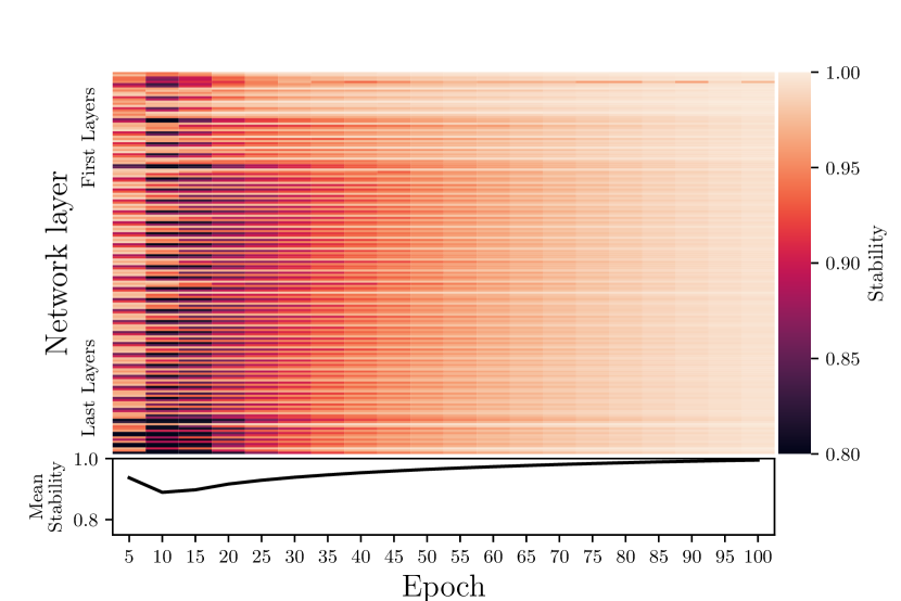
(a) ResNet-RS 101

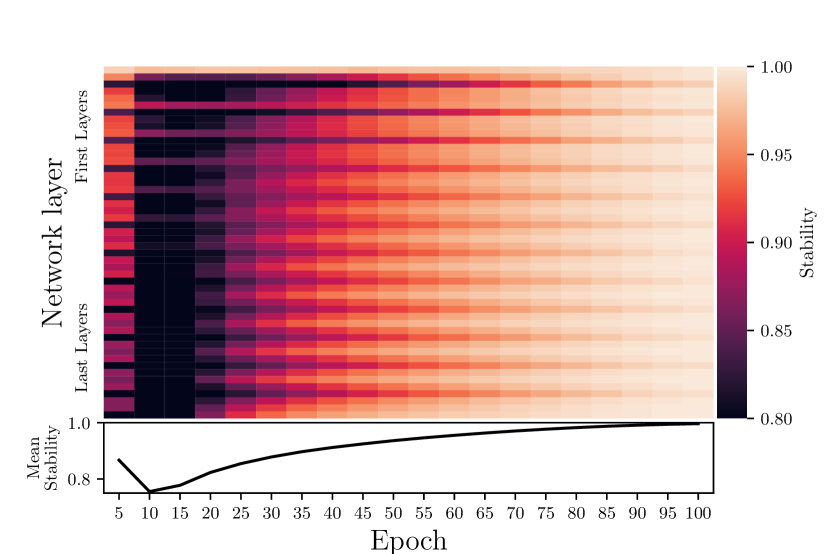
(b) Vision Transformer B/16

Figure 1: Stability, Equation 1, analysis of two different networks trained on the ImageNet-2012 dataset. Stability is measured at a frequency of five epochs, i.e., the bases of epoch $i$ are compared to the bases of epoch $i-5$. The x-axis shows the epoch number and the y-axis denotes the layer of the network, with layers closest to the input at the top. Darker colors indicate lower Stability, while lighter colors indicate higher Stability. The mean Stability for each epoch is shown beneath each heatmap.

Like any real-valued multidimensional matrix, each of a neural network’s weight matrices can be decomposed into orthogonal and linear mixing matrices. We postulate that these orthogonal bases tend to become less variable as the network trains.

We test our hypothesis by determining each weight’s orthogonal basis using the semi-orthogonal bases from its compact SVD. Compact SVD loosens the orthogonality constraints on ${\bm{U}}$ and ${\bm{V}}$ to only semi-orthogonal in the column dimension to reduce the inner dimension $r$. More precisely, it factorizes a matrix ${\bm{M}}\in\mathbb{R}^{m\times n}$ into ${\bm{U}}_{m\times r}{\bm{\Sigma}}_{r\times r}{\bm{V}}_{r\times n}^{T}$, where ${\bm{\Sigma}}$ is a diagonal matrix with the singular values along its diagonal, ${\bm{U}}$ and ${\bm{V}}$ are semi-orthogonal matrices consisting of orthogonal column vectors and non-orthogonal rows, and $r\leq\textrm{min}\left(m,n\right)$. To obtain a two-dimensional (2D) representation of a weight tensor with more than two dimensions, we maintain the original weight’s leading dimension and collapse those remaining. If the resulting 2D weight representation’s leading dimension is smaller than its second dimension (i.e. a short-fat matrix), we use its transpose. We then find a compact SVD of this representation to obtain the orthogonal bases. While the SVD of ${\bm{M}}$ is not unique, ${\bm{U}}{\bm{V}}^{T}$ is uniquely determined by ${\bm{M}}({\bm{M}}^{T}{\bm{M}})^{-1/2}$ and thus both unique and orthogonal.

To compare a weight’s bases at two distinct times during training, $i$ and $j$, we define their relative Stability $S_{ij}$ as:

$$S_{ij}=\mathrm{tr}\left(\left({\bm{U}}{\bm{V}}^{T}\right)_{i}\left({\bm{V}}{\bm{U}}^{T}\right)_{j}\right)/m$$ (1)

where $\mathrm{tr}$ is the trace, $({\bm{U}}{\bm{V}}^{T})_{k}$ represents the basis at a given time during training, and $m$ is the leading dimension of ${\bm{U}}$. Figure 1 shows how the Stability of the weights evolves for two vastly different network architectures, ResNet-RS 101 Bello et al. (2021) and the VisionTransformer (ViT) B/16 Dosovitskiy et al. (2021), trained on ImageNet-2012 Russakovsky et al. (2015). In both cases, the relative Stability decreases in the first 10 epochs, i.e. the bases vectors are changing, as the networks move away from their random initalizations. Then, the relative Stability increases towards 1, i.e. the bases vectors are not changing, over the remaining training time.

General patterns quickly emerge from these figures: the weights closer to the output stabilize faster than those toward the input, the stabilization rate differs depending on the layer type, and Stability increases throughout training. These observations intuitively make sense: the updates for weights closer to the network’s output will have fewer layer terms, thus the weights will get more direct responses for their ‘mistakes’; as we move towards the end of training each layer has learned most of how it responds to inputs.

We posit that the stabilization of the orthogonal bases during network training is crucial to the optimization process. Intuitively, this process resembles language learning Chomsky (1972). First, one develops a feeling for the language by acquiring a basic vocabulary and some phrases. Later, they delve into more complex grammar. Once the grammar patterns are internalized, there is no need to re-learn them; instead, one focuses on applying them in context. Similarly, neural networks first grasp the essential aspects of the task, then discern the roles of each layer, and eventually refine each layer’s operations to effectively perform its role.

4 Orthogonality-Informed Adaptive Low-Rank Training

To harness the stabilization of the orthogonal bases in neural network training, we present a novel algorithm that reduces the number of trainable parameters while maintaining both accuracy and overall time-to-train, unlike most previous methods which focused on either one or the other Xu and McAuley (2023).

As shown in Figure 1, most layers’ bases do not stabilize before a few epochs have passed. Therefore, we start training in a traditional full-rank scheme. After a number of iterations $d$, a hyperparameter of the algorithm, we transition the network’s multidimensional weights to their ${\bm{U}}\Sigma{\bm{V}}^{T}$ representation via their SVD. Experimentally, we found that the delay should be one third of the total number of iterations. At this point, we no longer train ${\bm{U}}$ and ${\bm{V}}^{T}$ with backpropagation but train only the square matrix ${\bm{\Sigma}}$. After a specified number of training steps $\nu$, the bases ${\bm{U}}$ and ${\bm{V}}^{T}$ are updated by extracting the new bases from the trained ${\bm{\Sigma}}$ matrix using an SVD of ${\bm{\Sigma}}$, as outlined in Algorithm 1.

Algorithm 1 Updating a weight matrix’s basis and cobasis, ${\bm{U}}$ and ${\bm{V}}$, from its actively trained singular value matrix ${\bm{\Sigma}}$. ${\bm{U}}$, ${\bm{\Sigma}}$, and ${\bm{V}}$ comprise the current ${\bm{U}}{\bm{\Sigma}}{\bm{V}}^{T}$ representation of a weight matrix.

Inputs: Frozen bases ${\bm{U}}$ and ${\bm{V}}$, trained ${\bm{\Sigma}}$ matrix

1:  ${\bm{U}}^{{}^{\prime}},{\bm{\Sigma}}^{{}^{\prime}},{\bm{V}}^{{}^{\prime}T}\leftarrow\texttt{SVD}({\bm{\Sigma}})$

2:  ${\bm{U}}\leftarrow{\bm{U}}{\bm{U}}^{{}^{\prime}},{\bm{V}}^{T}\leftarrow{\bm{V}}^{{}^{\prime}T}{\bm{V}}^{T},{\bm{\Sigma}}\leftarrow{\bm{\Sigma}}^{{}^{\prime}}$

After the basis ${\bm{U}}$ and cobasis ${\bm{V}}^{T}$ are updated, a new inner rank is found by removing the singular values whose absolute magnitude is less than $\beta$ times the largest singular value in the current ${\bm{\Sigma}}$, where $\beta$ is a hyperparameter that defaults to $0.1$. As the first layers of the network are generally unstable for longer, the update of ${\bm{U}}$ and ${\bm{V}}$ is only applied to the network’s last $\ell=L\cdot\alpha\cdot u$ layers, where $L$ is the number of network layers, $\alpha$ is a hyperparameter defaulting to $0.1$, and $u$ is the number of already completed updates. This process repeats until the end of training. Optionally, the first or last layers can be excluded from low-rank training depending on the use case. We provide an outline of our Orthogonality-Informed Adaptive Low-Rank (OIALR) training in Algorithm 2.

The first transition to the ${\bm{U}}\Sigma{\bm{V}}^{T}$ representation will almost certainly utilize more memory than in its traditional state. For example, a traditional weight matrix has $\mathcal{O}(mn)$ elements while the ${\bm{U}}\Sigma{\bm{V}}^{T}$ representation in OIALR has $\mathcal{O}\left(r(m+r+n)\right)$ elements, where $r$ is the inner rank. As training progresses, the number of ‘useful’ basis vectors is expected to decrease, resulting in a reduction in the network’s size, given that the network is trained appropriately.

Algorithm 2 OIALR training method

Inputs: Model $M$, training steps $t_{\max}$, delay steps $d$, low-rank update frequency $\nu$, singular value cutoff fraction $\beta$, percentage of layers in each low-rank update step size $\alpha$
Parameter: $L\leftarrow\text{Number of possible low-rank weights in }M$
Parameter: $\ell\leftarrow L\cdot\alpha$

1:  for $t\leftarrow 1$ to $t_{\max}$ do

2:     if $t<d$ then

3:        Train full-rank network.

4:     else if $t=d$ then

5:        Convert network to ${\bm{U}}{\bm{\Sigma}}{\bm{V}}^{T}$ representation.

6:     else if $t\texttt{ mod }\nu=0$ then

7:        for $i\leftarrow L-\ell$ to $L$ do

8:           Update ${\bm{U}}{\bm{\Sigma}}{\bm{V}}^{T}$ rep. $i$ with Algorithm 1.

9:           Remove singular values $<\beta\cdot\texttt{max}({\bm{\Sigma}}_{i})$

10:           Reshape ${\bm{U}}_{i}$, ${\bm{V}}_{i}$, ${\bm{\Sigma}}_{i}$, and optimizer states.

11:        $\ell\leftarrow\ell+L\cdot\alpha$

12:     else

13:        Train network’s ${\bm{U}}{\bm{\Sigma}}{\bm{V}}^{T}$ representations (${\bm{\Sigma}}$).

5 Experiments

To evaluate the effectiveness of our OIALR training approach, we conducted extensive experiments using different neural network architectures and datasets. Our primary focus was to demonstrate its effectiveness in terms of reducing the number of trainable parameters while maintaining or enhancing network performance and training time.

In our first experiment, we aim to understand what a typical researcher would experience by applying OIALR directly to a conventional and well-known neural network setup for a computer vision problem (see Section 5.2). Next, we compare OIALR to other popular low-rank and sparse methods (see Section 5.3). To see how OIALR performs on a real-world application, we investigate its performance in time-series forecasting with the Autoformer Wu et al. (2021), which was deployed at the 2022 Winter Olympics.

Up to this point, the hyperparameters (HPs) of the training methods are the same for both the baseline and OIALR methods. Given that OIALR dynamically alters the network structure during training, we expect the optimal HPs for OIALR training to vary from those used for full-rank training. For the final two experiments in Sections 5.4 and 5.5, we also determine more well-suited HPs for OIALR using Propulate Taubert et al. (2023), an asynchronous evolutionary optimization package shown to be effective for neural architecture searches Coquelin et al. (2021). We report ‘Compression’ and ‘Trainable parameters’ as percentages relative to the conventional model. For example, a compression of 80% signifies 20% fewer total parameters than the traditional model. Non-trainable parameters for OIALR-trained models are dominated by the ${\bm{U}}$ and ${\bm{V}}$ bases, while traditional models tend to have fewer non-trainable parameters like the running average in a batch normalization layer.

To demonstrate how our method would perform on real-world use cases, our experiments used state-of-the-art techniques and models, including strong image transforms Touvron et al. (2021), dropout Nitish et al. (2014), learning rate warm-up Gotmare et al. (2019), and cosine learning rate decay Loshchilov and Hutter (2017), implemented as per Wightman et al. (2023). All networks were trained using the AdamW L. and H. (2018) optimizer. Complete sets of HPs are included in Appendix A. Results represent the average of three runs with distinct random seeds.

5.1 Computational Environment

We ran all experiments on a distributed-memory, parallel hybrid supercomputer. Each compute node is equipped with two 38-core Intel Xeon Platinum 8368 processors at $2.4\text{\,}\mathrm{GHz}$ base and $3.4\text{\,}\mathrm{GHz}$ maximum turbo frequency, $512\text{\,}\mathrm{GB}$ local memory, a local $960\text{\,}\mathrm{GB}$ NVMe SSD disk, two network adapters, and four NVIDIA A100-40 GPUs with $40\text{\,}\mathrm{GB}$ memory connected via NVLink. Inter-node communication uses a low-latency, non-blocking NVIDIA Mellanox InfiniBand 4X HDR interconnect with $200\text{\,}\mathrm{G}\mathrm{bit}\mathrm{/}\mathrm{s}$ per port. All experiments used Python 3.10.6 with CUDA-enabled PyTorch 2.0.0 Paszke et al. (2019).

5.2 Vision Transformer on ImageNet-2012

Table 1: Training ViT-B/16 on ImageNet-2012 with and without OIALR. Hyperparameters are identical in both cases.

	Training method	Loss	Top-1 acc.	Top-5 acc.	Time to train	Compression	Trainable parameters
ViT-B/16	Baseline	2.16	71.64 %	89.18 %	3.29 $\mathrm{h}$	—	—
	OIALR	2.20	70.30 %	88.73 %	3.26 $\mathrm{h}$	98.95 %	16.56 %
ResNet-RS 101	Baseline	1.78	78.75 %	94.21 %	5.55 $\mathrm{h}$	—	—
	OIALR	1.81	77.95 %	93.95 %	5.92 $\mathrm{h}$	104.66 %	15.66 %

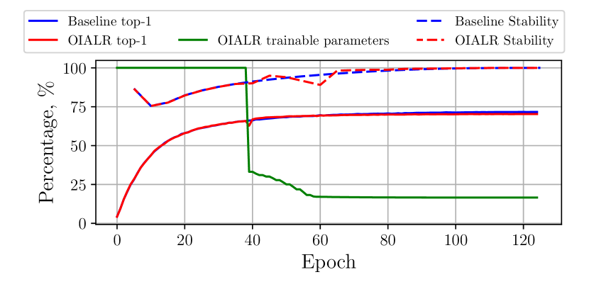
(a) Top-1 validation accuracy, percentage of trainable parameters as compared to the traditional network, and average Stability measured with a five-epoch frequency.

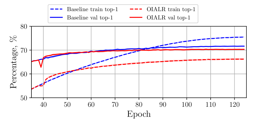
(b) Top-1 accuracies for training and validation with baseline and OIALR training methods.

Figure 2: Training of a ViT-B/16 network on ImageNet-2012 over 125 epochs.

For the first experiment, we trained the Vision Transformer (ViT)-B/16 model Dosovitskiy et al. (2021) on the ImageNet-2012 dataset Beyer et al. (2020) using the ReaL validation labels Beyer et al. (2020). The considerable parameter count of this model provided a rigorous test for the OIALR training method. We maintained identical HPs for both full-rank and adaptive low-rank training. To reduce the environmental impact, we trained for 125 epochs instead of the original 300 Dosovitskiy et al. (2021). By this point, validation accuracy had nearly stabilized, as shown in Figure 2(b). Additionally, we used an image resolution of $160\times 160$ instead of $224\times 224$ to further reduce the energy consumption.

The results are shown in Figure 2 and Table 1. Figure 2(a) presents the top-1 validation score, the percentage of trainable parameters relative to the full-rank model, and the average network Stability (as shown in Figure 1) throughout training. Notably, the baseline Stability increases smoothly throughout training, while OIALR’s Stability is less consistent due to the reductions in the weights’ ranks. This arises from the fact that the ${\bm{U}}{\bm{V}}^{T}$ from five epochs prior contains more basis vectors than the current ${\bm{U}}{\bm{V}}^{T}$.

As evident in Figure 2(b), there is a momentary accuracy drop when the network transitions from full-rank to its ${\bm{U}}{\bm{\Sigma}}{\bm{V}}^{T}$ representation, but it swiftly rebounds, surpassing previous performance. We theorize that this is caused by the residual momentum states in the optimizer ‘pushing’ the network in different directions.

In this untuned case, OIALR training required approximately the same amount of time to train ( $1\text{\,}\mathrm{\char 37\relax}$ longer) while the models maintained similar performance ($1.34(0.39)\text{\,}\mathrm{\char 37\relax}$ decrease in top-1 accuracy) than traditional full-rank training. OIALR reduced the number of trainable parameters to $16.56(0.23)\text{\,}\mathrm{\char 37\relax}$ of the full-rank parameters. Figure 2(b) shows that the full-rank model has entered the overfitting regime, where training accuracy continues increasing while validation accuracy plateaus, whereas the low-rank model has not.

5.3 Comparison with Related Low-Rank and Sparse Training Methods

To show where OIALR fits into the landscape of full-to-low-rank, low-rank, and sparse training methods, we performed a comparative analysis shown in Table 2. In these experiments, the baseline and compression methods use the same HPs.

OIALR and DLRT Schotthöfer et al. (2022) are SVD-based low-rank factorization methods. LRNN Idelbayev and Carreira-Perpiñán (2020) uses a traditional two-matrix representation (${\bm{W}}\approx{\bm{A}}{\bm{B}}$). CP He et al. (2017), SFP He et al. (2018), PP-1 Singh et al. (2019), and ThiNet Luo et al. (2017) are structured pruning methods which use channel or filter pruning for convolution layers. GAL Lin et al. (2019) and RNP Lin et al. (2017) are unstructured pruning methods; RigL Evci et al. (2020) is a sparse training method.

Overall, OIALR demonstrates competitive performance across different architectures and datasets. Despite producing subpar results on ResNet-50, it showed a marginal accuracy improvement over the baseline for VGG16 Liu and Deng (2015) on CIFAR-10. We theorize that since VGG16 is known to be over-parameterized, there are more basis vectors that can be removed. By eliminating these less useful basis vectors, the network can focus on those remaining to train a performant low-rank network.

Table 2: Comparison of OIALR with various compression methods. ‘Diff. to baseline’ refers to the difference in top-1 validation (ImageNet-2012) or test (CIFAR-10) accuracy between the baseline and the listed methods. Positive values indicate that the listed method outperforms the traditionally trained network. Absence of data indicated by ‘—’. For non-OIALR results see Schotthöfer et al. (2022); Evci et al. (2020).

	Training method	Diff. to baseline	Compression	Trainable parameters
ResNet-50 ImageNet-2012	OIALR	-1.72 %	82.55 %	15.15 %
	DLRT	-0.56 %	54.10 %	14.20 %
	PP-1	-0.20 %	44.20 %	—
	CP	-1.40 %	50.00 %	—
	SFP	-0.20 %	41.80 %	—
	ThiNet	-1.50 %	36.90 %	—
	RigL	-2.20 %	20.00 %	—
VGG16 ImageNet-2012	OIALR	-1.53 %	36.52 %	4.77 %
	DLRT	-2.19 %	86.00 %	78.40 %
	PP-1	-0.19 %	80.20 %	—
	CP	-1.80 %	80.00 %	—
	ThiNet	-0.47 %	69.04 %	—
	RNP(3X)	-2.43 %	66.67 %	—
VGG16 CIFAR-10	OIALR	0.10 %	27.05 %	13.88 %
	DLRT	-1.89 %	56.00 %	77.50 %
	GAL	-1.87 %	77.00 %	—
	LRNN	-1.90 %	60.00 %	—

5.4 Ablation Study on Mini ViT on CIFAR-10

Table 3: A mini ViT trained on CIFAR-10. ‘OIALR, tuned’ training runs used tuned HPs, while ‘OIALR’ used the same HPs as the baseline. Accuracies and loss values are determined on the test dataset.

Training method	Loss	Top-1 accuracy	Top-5 accuracy	Time to train	Compression	Trainable parameters
Traditional	0.88	85.17 %	98.34 %	12.14 $\min$	—	—
OIALR	0.91	83.05 %	98.38 %	11.99 $\min$	146.78 %	30.98 %
OIALR, tuned	0.85	86.33 %	98.53 %	11.19 $\min$	55.06 %	9.97 %

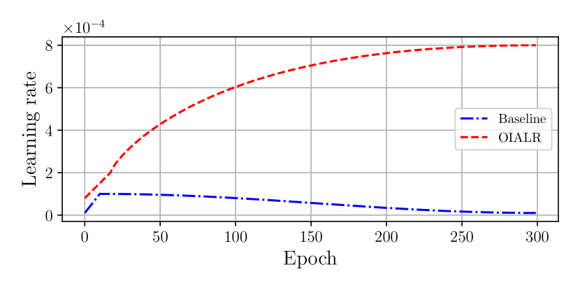
Figure 3: Learning rate schedules for baseline and OIALR training for a mini ViT on CIFAR-10. OIALR training learning rate schedule determined by HP search.

To show how OIALR performs with proper tuning, we trained a reduced-size ViT model on the CIFAR-10 dataset with and without tuning. The runs without tuning use the same HPs as the baseline runs. As reduced-size ViT models have been shown to perform superbly Hassani et al. (2022) at a fraction of the compute time, we elect to use a ViT-B/16 variant with a patch size of eight, six layers, and six attention heads in this experiment (original values are a patch size of 16, 12 layers, and 12 attention heads). The results of this experiment are shown in Table 3 and Figure 3.

Interestingly, the best learning rate schedule for the OIALR training method discovered through HP search increases the learning rate as the number of parameters decreases, see Figure 3. This result makes intuitive sense: as the number of trainable parameters decreases, the learning rate applied to the gradients of the remaining parameters can be increased without the model degrading.

Although the untuned OIALR model reduced the trainable parameters by $69.02(0.07)\text{\,}\mathrm{\char 37\relax}$, the top-1 test accuracy dropped by over $2\text{\,}\mathrm{\char 37\relax}$. In contrast, the tuned OIALR model reduced the number of trainable parameters by $90.03(0.13)\text{\,}\mathrm{\char 37\relax}$ while increasing predictive performance over the baseline from $85.17(0.42)\text{\,}\mathrm{\char 37\relax}$ to $86.33(0.71)\text{\,}\mathrm{\char 37\relax}$. Furthermore, training time was reduced by $8.52(0.82)\text{\,}\mathrm{\char 37\relax}$ over the baseline.

5.5 Ablation Study on Autoformer on ETTm2

Table 4: Training of the Autoformer model on the ETTm2 dataset. Baseline and untuned OIALR HPs were the default parameters from Wu et al. (2021). Tuned OIALR HPs were found via Propulate. Prediction lengths (PL) in the leftmost column are in $15\text{\,}\min$ time steps. The optimal value for mean squared error (MSE) and mean absolute error (MAE) is zero.

PL	Training method	MSE	MAE	Compression	Trainable parameters
96	Baseline	0.2145	0.2994	—	—
	OIALR	0.2140	0.2974	182.06 %	46.16 %
	OIALR, tuned	0.2112	0.2942	47.84 %	12.19 %
192	Baseline	0.2737	0.3356	—	—
	OIALR	0.2773	0.3336	163.35 %	105.31 %
	OIALR, tuned	0.2686	0.3305	105.31 %	27.15 %
336	Baseline	0.3277	0.3640	—	—
	OIALR	0.3253	0.3863	179.87 %	45.67 %
	OIALR, tuned	0.3212	0.3591	27.30 %	7.14 %
720	Baseline	0.4194	0.4157	—	—
	OIALR	0.4213	0.4186	194.13 %	51.33 %
	OIALR, tuned	0.4120	0.4147	13.55 %	4.46 %

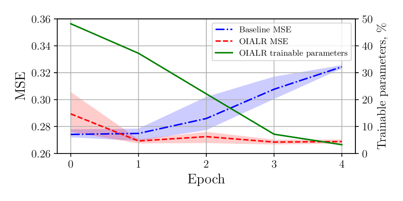
(a) Prediction length 192

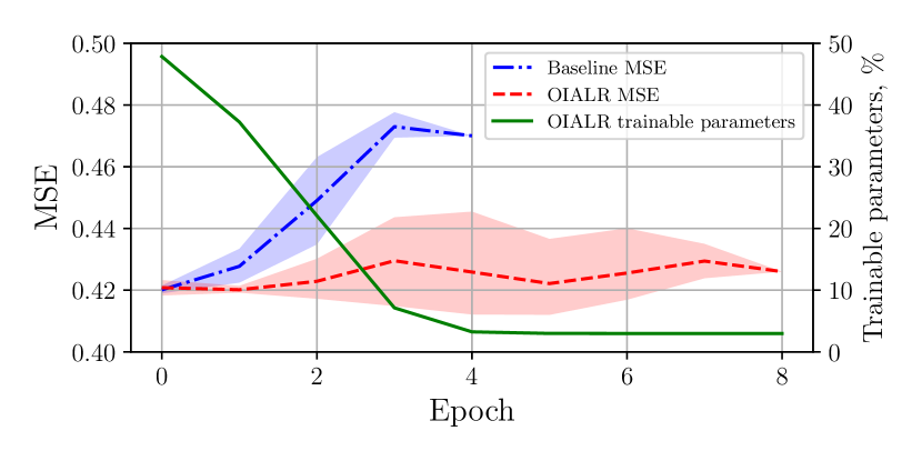
(b) Prediction length 720

Figure 4: MSE and the percentage of trainable parameters relative to the full-rank model for the Autoformer trained on the ETTm2 dataset using two different prediction lengths in $15\text{\,}\min$ time steps.

This use case serves as a crucial test for the OIALR method, showcasing its versatility by applying it to a model in a radically different domain. Furthermore, it validates that the findings depicted in Figure 1 remain applicable in non-image scenarios.

The Electricity Transformer Dataset Zhou et al. (2021) (ETT) measures load and oil temperature of electrical transformers. It contains 70,000 measurements at various levels of granularity, each with seven features, and is primarily used for time series forecasting. We focus on the ETTm2 dataset, which has a 15-minute resolution. Common prediction lengths for this dataset are 96, 192, 336, and 720 time steps. The Autoformer Wu et al. (2021), a well-known transformer model in Hugging Face’s repository, differs from the other tested transformers by using auto-correlation layers and one-dimensional convolutions. Due to its success, it was deployed at the 2022 Winter Olympics for weather forecasting.

Given the baseline’s susceptibility to overfitting (see Figure 4), we initiate training in low rank instead of transitioning during training. Although some overfitting is observed in the OIALR results, it is considerably less severe than in the baseline. As Table 4 indicates, the tuned OIALR models were more accurate across all prediction lengths with a drastically decreased number of parameters.

The untuned OIALR models outperformed the baseline in some cases and succeeded in reducing the number of trainable parameters to $45.72\text{\,}\mathrm{\char 37\relax}$ on average. As explained in Section 4, these models required more parameters than the baseline model due to the shapes of the model’s ${\bm{U}}{\bm{\Sigma}}{\bm{V}}^{T}$ representation. The tuned OIALR measurements generally showed a much more successful compression percentage. Interestingly, the tuned OIALR model required more trainable parameters for predicting shorter time spans.

In contrast to the previous experiment, the best learning rate scheduler found for this use case more closely resembles a traditional scheduler, featuring a warm-up phase followed by a gradual decay. This may be related to the fact that the networks, both low-rank and full-rank, overfit the training dataset quickly.

6 Conclusion

There has long been curiosity about how a neural network learns. This study aimed to shed light on this question by exploring the nature of neural network weights during training through their singular value decomposition. Our findings revealed that the orthogonal component of a neural network’s weights stabilizes early in the training process. Building on this discovery, we introduced Orthogonality-Informed Adaptive Low-Rank (OIALR) training.

We evaluated OIALR by training low-rank versions of widely used and state-of-the-art neural networks across diverse data modalities and tasks. OIALR demonstrated superior performance when compared against other low-rank methods, even when employing the default hyperparameter settings used in traditional model training. While our approach may not directly surpass traditional training techniques in all scenarios, it can outperform them in terms of both accuracy and training time when tuned appropriately.

OIALR’s true strength lies in substantially reducing the number of trainable parameters of the final model, thereby facilitating model fine-tuning, transfer learning, and deployment on resource-constrained devices. This reduction also contributes to reducing the data transfer requirements during distributed training, reducing the gap between expensive, top-tier clusters and more affordable options.

Integrating orthogonality-based training methods into the deep learning researcher’s toolkit offers promising possibilities for a wide range of applications. With this work, we hope to inspire further exploration and refinement of orthogonality-informed methods, ultimately advancing the field of machine learning and its practicality across diverse domains.

Ethical Statement

There are no ethical issues to report.

References

- Bejani and Ghatee [2020] M. M. Bejani and M. Ghatee. Adaptive Low-Rank Factorization to regularize shallow and deep neural networks, May 2020. arXiv:2005.01995 [cs, stat].
- Bello et al. [2021] I. Bello, W. Fedus, X. Du, et al. Revisiting ResNets: Improved Training and Scaling Strategies, March 2021. arXiv:2103.07579 [cs].
- Beyer et al. [2020] L. Beyer, O. J. Hénaff, A. Kolesnikov, et al. Are we done with ImageNet?, June 2020. arXiv:2006.07159 [cs].
- Cahyawijaya et al. [2021] S. Cahyawijaya, G. I. Winata, H. Lovenia, et al. Greenformer: Factorization Toolkit for Efficient Deep Neural Networks, October 2021. arXiv:2109.06762 [cs].
- Ceruti et al. [2021] G. Ceruti, J. Kusch, and C. Lubich. A rank-adaptive robust integrator for dynamical low-rank approximation, April 2021. arXiv:2104.05247 [cs, math].
- Chomsky [1972] C. Chomsky. Stages in Language Development and Reading Exposure. Harvard Educational Review, 42(1):1–33, April 1972.
- Coquelin et al. [2021] D. Coquelin, R. Sedona, M. Riedel, and M. Götz. Evolutionary Optimization of Neural Architectures in Remote Sensing Classification Problems. In 2021 IEEE International Geoscience and Remote Sensing Symposium IGARSS, pages 1587–1590, July 2021. ISSN: 2153-7003.
- Deng et al. [2020] L. Deng, G. Li, S. Han, L. Shi, and Y. Xie. Model Compression and Hardware Acceleration for Neural Networks: A Comprehensive Survey. Proceedings of the IEEE, 108(4):485–532, April 2020. Conference Name: Proceedings of the IEEE.
- Dosovitskiy et al. [2021] A. Dosovitskiy, L. Beyer, A. Kolesnikov, et al. An Image is Worth 16x16 Words: Transformers for Image Recognition at Scale, June 2021. arXiv:2010.11929 [cs] version: 2.
- Evci et al. [2020] U. Evci, T. Gale, J. Menick, et al. Rigging the Lottery: Making All Tickets Winners. In Proceedings of the 37th International Conference on Machine Learning, ICML’20. JMLR.org, 2020.
- Gotmare et al. [2019] A. Gotmare, N. Shirish Keskar, C. Xiong, and R. Socher. A Closer Look at Deep Learning Heuristics: Learning rate restarts, Warmup and Distillation. In International Conference on Learning Representations, 2019.
- Guo et al. [2023] T. Guo, N. Yolwas, and W. Slamu. Efficient Conformer for Agglutinative Language ASR Model Using Low-Rank Approximation and Balanced Softmax. Applied Sciences, 13(7):4642, January 2023. Number: 7 Publisher: Multidisciplinary Digital Publishing Institute.
- Hassani et al. [2022] A. Hassani, S. Walton, N. Shah, et al. Escaping the Big Data Paradigm with Compact Transformers, June 2022. arXiv:2104.05704 [cs] version: 4.
- He et al. [2017] Y. He, X. Zhang, and J. Sun. Channel Pruning for Accelerating Very Deep Neural Networks. In 2017 IEEE International Conference on Computer Vision (ICCV), pages 1398–1406, 2017.
- He et al. [2018] Y. He, G. Kang, X. Dong, et al. Soft Filter Pruning for Accelerating Deep Convolutional Neural Networks. In Proceedings of the 27th International Joint Conference on Artificial Intelligence, IJCAI’18, page 2234–2240. AAAI Press, 2018.
- Hssayni et al. [2022] E. h. Hssayni, N.-E. Joudar, and M. Ettaouil. KRR-CNN: kernels redundancy reduction in convolutional neural networks. Neural Computing and Applications, 34(3):2443–2454, February 2022.
- Hsu et al. [2022] Y.-C. Hsu, T. Hua, S. Chang, et al. Language model compression with weighted low-rank factorization. In International Conference on Learning Representations, 2022.
- Hu et al. [2022] E. J. Hu, Y. Shen, P. Wallis, et al. LoRA: Low-rank adaptation of large language models. In International Conference on Learning Representations, 2022.
- Idelbayev and Carreira-Perpiñán [2020] Y. Idelbayev and M. Á. Carreira-Perpiñán. Low-Rank Compression of Neural Nets: Learning the Rank of Each Layer. In 2020 IEEE/CVF Conference on Computer Vision and Pattern Recognition (CVPR), pages 8046–8056, June 2020. ISSN: 2575-7075.
- L. and H. [2018] Ilya L. and Frank H. Fixing Weight Decay Regularization in Adam, 2018.
- Lin et al. [2017] J. Lin, Y. Rao, J. Lu, and J. Zhou. Runtime Neural Pruning. In I. Guyon, U. Von Luxburg, S. Bengio, H. Wallach, R. Fergus, S. Vishwanathan, and R. Garnett, editors, Advances in Neural Information Processing Systems, volume 30. Curran Associates, Inc., 2017.
- Lin et al. [2019] S. Lin, R. Ji, C. Yan, et al. Towards Optimal Structured CNN Pruning via Generative Adversarial Learning. In 2019 IEEE/CVF Conference on Computer Vision and Pattern Recognition (CVPR), pages 2785–2794, 2019.
- Liu and Deng [2015] Shuying Liu and Weihong Deng. Very deep convolutional neural network based image classification using small training sample size. In 2015 3rd IAPR Asian Conference on Pattern Recognition (ACPR), pages 730–734, 2015.
- Loshchilov and Hutter [2017] I. Loshchilov and F. Hutter. SGDR: Stochastic Gradient Descent with Warm Restarts, May 2017. arXiv:1608.03983 [cs, math].
- Luo et al. [2017] J.-H. Luo, J. Wu, and W. Lin. ThiNet: A Filter Level Pruning Method for Deep Neural Network Compression. In 2017 IEEE International Conference on Computer Vision (ICCV), pages 5068–5076, 2017.
- Mahabadi et al. [2021] Rabeeh Karimi Mahabadi, James Henderson, and Sebastian Ruder. Compacter: Efficient low-rank hypercomplex adapter layers. In A. Beygelzimer, Y. Dauphin, P. Liang, and J. Wortman Vaughan, editors, Advances in Neural Information Processing Systems, 2021.
- Nitish et al. [2014] S. Nitish, G. Hinton, A. Krizhevsky, et al. Dropout: A Simple Way to Prevent Neural Networks from Overfitting. Journal of Machine Learning Research, 15(56):1929–1958, 2014.
- Paszke et al. [2019] A. Paszke, S. Gross, F. Massa, et al. Pytorch: An imperative style, high-performance deep learning library. In Advances in Neural Information Processing Systems, volume 32. Curran Associates, Inc., 2019.
- Phan et al. [2020] A.-H. Phan, K. Sobolev, K. Sozykin, et al. Stable Low-Rank Tensor Decomposition for Compression of Convolutional Neural Network. In A. Vedaldi, H. Bischof, T. Brox, and J.-M. Frahm, editors, Computer Vision – ECCV 2020, Lecture Notes in Computer Science, pages 522–539, Cham, 2020. Springer International Publishing.
- Povey et al. [2018] D. Povey, G. Cheng, Y. Wang, et al. Semi-Orthogonal Low-Rank Matrix Factorization for Deep Neural Networks. In Interspeech 2018, pages 3743–3747. ISCA, September 2018.
- Psichogios and Ungar [1994] D.C. Psichogios and L.H. Ungar. SVD-NET: an algorithm that automatically selects network structure. IEEE Transactions on Neural Networks, 5(3):513–515, May 1994. Conference Name: IEEE Transactions on Neural Networks.
- Russakovsky et al. [2015] O. Russakovsky, J. Deng, H. Su, et al. ImageNet Large Scale Visual Recognition Challenge. International Journal of Computer Vision, 115(3):211–252, December 2015.
- Schotthöfer et al. [2022] S. Schotthöfer, E. Zangrando, J. Kusch, et al. Low-rank lottery tickets: finding efficient low-rank neural networks via matrix differential equations. Advances in Neural Information Processing Systems, 35:20051–20063, December 2022.
- Singh et al. [2019] P. Singh, V. K. Verma, P. Rai, and V. P. Namboodiri. Play and Prune: Adaptive Filter Pruning for Deep Model Compression. In Proceedings of the 28th International Joint Conference on Artificial Intelligence, IJCAI’19, page 3460–3466. AAAI Press, 2019.
- Taubert et al. [2023] O. Taubert, M. Weiel, D. Coquelin, et al. Massively parallel genetic optimization through asynchronous propagation of populations. In International Conference on High Performance Computing, pages 106–124. Springer, 2023.
- Touvron et al. [2021] H. Touvron, M. Cord, M. Douze, et al. Training data-efficient image transformers & distillation through attention. In M. Meila and T. Zhang, editors, Proceedings of the 38th International Conference on Machine Learning, volume 139 of Proceedings of Machine Learning Research, pages 10347–10357. PMLR, 18–24 Jul 2021.
- Waleffe and Rekatsinas [2020] R. Waleffe and T. Rekatsinas. Principal Component Networks: Parameter Reduction Early in Training. CoRR, abs/2006.13347, 2020.
- Wang et al. [2020] Ziheng Wang, Jeremy Wohlwend, and Tao Lei. Structured pruning of large language models. In Bonnie Webber, Trevor Cohn, Yulan He, and Yang Liu, editors, Proceedings of the 2020 Conference on Empirical Methods in Natural Language Processing (EMNLP), pages 6151–6162, Online, November 2020. Association for Computational Linguistics.
- Wightman et al. [2023] R. Wightman, N. Raw, A. Soare, et al. rwightman/pytorch-image-models: v0.8.10dev0 Release, February 2023.
- Winata et al. [2020] G. I. Winata, S. Cahyawijaya, Z. Lin, Z. Liu, and P. Fung. Lightweight and Efficient End-To-End Speech Recognition Using Low-Rank Transformer. In ICASSP 2020 - 2020 IEEE International Conference on Acoustics, Speech and Signal Processing (ICASSP), pages 6144–6148, May 2020. ISSN: 2379-190X.
- Wu et al. [2021] H. Wu, J. Xu, J. Wang, and M. Long. Autoformer: Decomposition Transformers with Auto-Correlation for Long-Term Series Forecasting. In Advances in Neural Information Processing Systems, 2021.
- Xu and McAuley [2023] C. Xu and J. McAuley. A Survey on Model Compression and Acceleration for Pretrained Language Models. Proceedings of the AAAI Conference on Artificial Intelligence, 37(9):10566–10575, June 2023. Number: 9.
- Xu et al. [2019] Yuhui Xu, Yuxi Li, Shuai Zhang, Wei Wen, Botao Wang, Wenrui Dai, Yingyong Qi, Yiran Chen, Weiyao Lin, and Hongkai Xiong. Trained Rank Pruning for Efficient Deep Neural Networks. In 2019 Fifth Workshop on Energy Efficient Machine Learning and Cognitive Computing - NeurIPS Edition (EMC2-NIPS), pages 14–17, 2019.
- Yang et al. [2021] Z. Yang, A. Zhang, and A. Sudjianto. Enhancing explainability of neural networks through architecture constraints. IEEE Transactions on Neural Networks and Learning Systems, 32(6):2610–2621, 2021.
- Zhang et al. [2023] B. Zhang, W. Zheng, J. Zhou, and J. Lu. Bort: Towards Explainable Neural Networks with Bounded Orthogonal Constraint. In The Eleventh International Conference on Learning Representations, 2023.
- Zhou et al. [2021] H. Zhou, S. Zhang, J. Peng, et al. Informer: Beyond Efficient Transformer for Long Sequence Time-Series Forecasting, March 2021. arXiv:2012.07436 [cs].