Faster ISNet for Background Bias Mitigation on Deep Neural Networks

Abstract

Image background features can constitute background bias (spurious correlations) and impact deep classifiers decisions, causing shortcut learning (Clever Hans effect) and reducing the generalization skill on real-world data. The concept of optimizing Layer-wise Relevance Propagation (LRP) heatmaps, to improve classifier behavior, was recently introduced by a neural network architecture named ISNet. It minimizes background relevance in LRP maps, to mitigate the influence of image background features on deep classifiers decisions, hindering shortcut learning and improving generalization. For each training image, the original ISNet produces one heatmap per possible class in the classification task, hence, its training time scales linearly with the number of classes. Here, we introduce reformulated architectures that allow the training time to become independent from this number, rendering the optimization process much faster. We challenged the enhanced models utilizing the MNIST dataset with synthetic background bias, and COVID-19 detection in chest X-rays, an application that is prone to shortcut learning due to background bias. The trained models minimized background attention and hindered shortcut learning, while retaining high accuracy. Considering external (out-of-distribution) test datasets, they consistently proved more accurate than multiple state-of-the-art deep neural network architectures, including a dedicated image semantic segmenter followed by a classifier. The architectures presented here represent a potentially massive improvement in training speed over the original ISNet, thus introducing LRP optimization into a gamut of applications that could not be feasibly handled by the original model.

Keywords: Shortcut learning, Layer-wise relevance propagation, COVID-19 detection, explainable artificial intelligence, background bias, ISNet

1 Introduction

Deep neural networks (DNNs) have dominated the field of computer vision, sometimes surpassing human performance. However, the deep models are flexible, non-linear, and contain millions of parameters. Thus, interpreting and controlling a DNN behavior is a complex endeavor. Shortcut learning[1] is a phenomenon that highlights the potential unpredictability of deep networks. It occurs when a network relies on shortcut features to minimize its training loss, instead of focusing on features that are truly relevant to the classification problem[1]. Shortcut features present in a specific training dataset are not on common real-world data. Therefore, a DNN suffering from shortcut learning will perform well on the training dataset, and on test data drawn from its data distribution. I.e., a test dataset independent and identically distributed, or i.i.d., in relation to the training data (such as test datasets obtained by randomly splitting a dataset into a train and a test partition). However, shortcut learning impairs generalization, reducing DNN accuracy on data generated by external sources with respect to the training database, known as out-of-distribution (o.o.d.) test datasets. Multiple characteristics of the training data can act as shortcut features, such as lighting, object position in the image, object orientation, and characteristics of the background[1]. For an image feature to be considered a shortcut, it must be correlated to the image class in the training dataset, but not be an intrinsic characteristic of that class, such that the correlation may not hold for o.o.d. data. Shortcuts and shortcut learning are also known as spurious correlations and ’Clever Hans effect’, respectively[1]. Shortcut features in the image’s background may also be called background bias. Shortcut learning is a problem that must be addressed for deep learning to become more trustworthy, a key quality for its utilization in critical applications, such as medical or security-related tasks.

A contemporary example of shortcut learning related to background bias can be observed in the task of COVID-19 classification with chest X-rays[2]^,[3]^,[4]^,[5]. Most COVID-19 X-ray databases[2]^,[4], including some of the largest datasets[6] (necessary for improving accuracy and generalization in deep learning), contain no or insufficient data from healthy patients (or other diseases of interest) gathered from the same hospitals that provided the COVID-19 X-rays. Therefore, researchers training neural networks commonly rely on mixed databases[2]^,[4]^,[3]: datasets that have diverse sources (hospitals and physical locations) for different classes (e.g., COVID-19, pneumonia and healthy). X-rays from different hospitals have diverse background characteristics. Such background particularities can even allow accurate source identification when the lungs (foreground) are removed from the image[7]. The X-ray background features are correlated to their sources, and, in a mixed dataset, to the image class. Consequently, they represent background bias. Accordingly, networks trained with these datasets performed very well (normally 95% to 100% accuracy) in standard i.i.d. test datasets, assembled from the same hospitals that provided the training data[3]. E.g., evaluation datasets produced with the standard machine learning procedure of randomly splitting a database into a train and a test division. However, these networks do not generalize well to data drawn from other hospitals, evidencing shortcut learning[2]^,[3]^,[4]. Moreover, a second evidence of shortcut learning caused by background bias is that studies could significantly increase o.o.d. test performance by removing the background from the X-rays[5]^,[4]. Besides COVID-19 detection, tuberculosis detection in chest X-rays is another task where dataset mixing is normally required, commonly resulting in background bias, shortcut learning and weak generalization[4]^,[8].

A common practice to train classifiers in datasets with background bias consists in using a segmentation-classification pipeline. A deep segmenter removes the image’s background, afterward, a classifier analyses the segmented image (without background). The model employs two deep neural networks in series, reducing its computational efficiency. In a previous work[4], we introduced the ISNet (Implicit Segmentation Neural Network), a deep classifier architecture that utilizes background relevance minimization (BRM) on Layer-wise Relevance Propagation[9] (LRP) heatmaps. Unlike the alternative segmentation-classification pipeline, the run-time ISNet constitutes a single neural network, making it faster and lighter[4]. The ISNet learns to identify and focus on the images’ foregrounds. Accordingly, the model was capable of reliably minimizing attention to background bias, hindering the shortcut learning caused by it, even considering high-dimensional data and very deep classification backbones (e.g., DenseNet121, with 121 layers)[4]. Besides being faster and lighter than the pipeline, the ISNet also surpassed the alternative model in terms of accuracy[4].

Layer-wise relevance propagation is a DNN explanation technique. It works by retro-propagating a signal (called relevance), utilizing multiple custom propagation rules[9]. The propagation starts from a single logit (DNN output score for a given class) and passes through all deep classifier layers. The procedure embeds high-level semantic information and precise spatial information (present at the different layers’ outputs) into a high-resolution heatmap. In the map, positive values (relevance) indicate input image features that improved the DNN confidence for the propagated logit’s class. Meanwhile, negative relevance points features that reduced this confidence. Finally, low relevance magnitude represents features that the DNN found irrelevant for the explained class[9].

The ISNet introduced the concept of directly optimizing of LRP heatmaps to improve a deep classifier’s behavior. The model produces differentiable heatmaps during training, and feeds them to the heatmap loss[4]. The function relies on segmentation masks to identify and penalize background attention in the heatmaps. By minimizing a linear combination of the heatmap loss and a classification loss (e.g., cross-entropy), the ISNet learns to focus its attention on the image’s foreground, ignoring background bias. This optimization procedure is called background relevance minimization, and it can be regarded as an explanation-based spatial attention mechanism. Importantly, the ISNet does not need LRP heatmaps or segmentation masks after training, ensuring that the run-time model has no extra computation cost in relation to a standard classifier. Thus, it can be efficiently deployed in portable or less powerful devices. Moreover, as LRP can be applied to virtually any DNN[10], including recurrent networks. Thus, background relevance minimization can be used with multiple classifier architectures.

The ISNet was capable of outperforming multiple state-of-the-art neural networks when dealing with background bias. The ISNet and the segmentation-classification pipeline were the only models that could consistently avoid the influence of synthetic background bias over the classifier’s decisions, hindering shortcut learning[4]. Moreover, the ISNet’s accuracy surpassed the large pipeline’s results, making it the best performing DNN. In tasks with non-synthetic background bias (COVID-19 and tuberculosis detection with mixed X-ray datasets), the ISNet was the network that best focused on the lungs[4]. By minimizing background attention, the model hindered shortcut learning. Thus, it significantly outperformed all alternative models in external (o.o.d.) test datasets. The benchmark models comprised standard classifiers and multiple state-of-the-art architectures designed to control classifier attention[4]. They are: models optimizing other explanation heatmaps, namely, input gradients[11] (RRR[12]), Gradient*Input[13] (ISNet Grad*Input ablation), and Grad-CAM[14] (GAIN[15] and HAM[16]); attention mechanisms that do not learn from semantic segmentation masks (vision transformers[17] and attention-gated neural networks[18]); the large segmentation-classification pipeline; and a multi-task neural network performing segmentation and classification simultaneously. The reasons for the ISNet’s superior performance are explained in detail in the past study[4], and summarized in Section 2.2 of this work. Besides empirically comparing the ISNet to multiple alternative methodologies, the study presenting the architecture theoretically justified its superior performance[4] (refer to Section 2.2).

A disadvantage of the original ISNet is the computational cost of its training procedure, which increases linearly with the number of classes in the classification problem[4]. E.g., training an ISNet for a classification task with C=100 classes takes roughly 10 times more time than for a problem with C=10 classes, considering the same DNN and dataset size. The ISNet minimizes background relevance in C LRP heatmaps per training image. Each heatmap is created by starting LRP from one of the DNN logits (i.e., in each heatmap the positive relevance is associated to one of the C possible classes). Thus, increasing the number of classes also increments the number of heatmaps. Multiple maps were required because one could not fully express the influence of background bias on the classifier[4]. A standard LRP heatmap explains how input features affected the DNN classification score (logit) for a given class. Thus, it may not indicate if bias influenced the logits for the remaining classes. For example, a heatmap explaining the predicted class could not show if a background feature lowered the classifier confidence for the losing classes, a behavior that could significantly affect the classifier’s decisions. When all possible heatmaps are produced and penalized separately, positive and negative background relevance can be minimized for all classes, ensuring DNN resistance to background bias[4].

This study proposes the Faster ISNet architecture family, which encompasses 3 reformulations of the ISNet architecture: the Dual ISNet (Section 2.4.2), the Selective ISNet (Section 2.4.1), and the Stochastic ISNet (Section 2.4.3). By redefining the LRP procedure the ISNet uses during training, the Faster ISNet removes the training time dependency on the number of classes in the application. The original ISNet separately propagates LRP relevance for all C classifier output neurons’ logits, using LRP-$\varepsilon$[9] propagation rules (and LRP-z^B in the first DNN layer)[4]. Meanwhile, the Dual ISNet propagates relevance for all logits simultaneously. To avoid a shortcut solution, it utilizes two separate relevance signals, one considers LRP-$\varepsilon$[10] rules, while the other employs LRP-z⁺[10] (propagating only positive relevance). Each of the two signals creates one heatmap, which is penalized by the ISNet heatmap loss[4]. Thus, the Dual ISNet produces two heatmaps per training sample, instead of C. The Selective ISNet LRP procedure does not propagate logits. Instead, it uses LRP-$\varepsilon$ to propagate a Softmax-based quantity, $\eta_{c}$[10], calculated for a single class (c). Thus, the model creates only one heatmap per training image. Finally, the Stochastic ISNet employs LRP-$\varepsilon$ to propagate relevance from DNN logits. However, it creates a single heatmap per training image, explaining a single logit. To prevent shortcut solutions, we proposed a stochastic selection procedure to select the explained logit (Section 2.4.3). In all new ISNet formulations, training computational cost is independent of the number of categories in the classification problem. The original ISNet’s training time was not excessively long for applications with a small number of classes, such as many biomedical classification tasks (like the ones in the paper presenting the model[4]). However, the Faster ISNet can vastly reduce training time in applications with more classes. Moreover, it makes LRP optimization feasible in applications where training the original ISNet would require an extremely long time and/or an excessive number of graphics processing units (GPUs), two scenarios associated with heavy electrical energy consumption and high cost.

Furthermore, due to the reduced training time, we can more efficiently apply LRP optimization to large classifier architectures. The classifiers in the original ISNet formulation[4] were Densely Connected Convolutional Networks (DenseNets), a remarkably efficient architecture, with a small number of parameters in relation to the neural network depth[19]. Moreover, the past study[4] also implemented VGG[20]-based ISNets. Besides experimenting with DenseNets, the current study introduces ISNets based on Residual Neural Networks (ResNets)[21], which require more parameters and take longer to train in relation to the DenseNets. However, ResNet-based networks are among the most popular and accurate architectures for very deep networks [21]. In summary, by greatly reducing the ISNet training time, we facilitate the utilization of multiple large architectures as ISNet backbones, especially in classification tasks with many classes. To further improve training efficiency, we developed a quick heuristic to determine two of the ISNet loss hyper-parameters (Section 2.3), accelerating hyper-parameter tuning.

We evaluate the Faster ISNet in two tasks. First, to create an objective experiment that allows a quantitative evaluation of shortcut learning, we added synthetic background bias to the MNIST handwritten digit classification database[22]. The bias is a background pixel, selected according to the image’s label and made white. Thus, it spuriously correlate with the image class. The dataset was projected to be simple and allow fast training (with 28x28 sized images), serving as a development platform for attention mechanisms that ignore background bias. The artificial bias is present in all training data, and there are three test datasets: the i.i.d. set, which contains the same artificial bias; the o.o.d. set, constituted of original (unbiased) MNIST images; and the deceiving bias dataset, where the correspondence between the positively-labeled class and the biasing pixel is altered in a deceitful manner (e.g., a biasing pixel that was associated to class 2 in training becomes correlated to class 3). The three test datasets allow the quantitative evaluation of the shortcut learning induced by background bias: the more the synthetic bias influences the classifier, the higher the performance drop we observe when comparing accuracy on the i.i.d. test dataset, to the performance on the o.o.d. and deceiving bias test sets. This performance drop represents a generalization gap to o.o.d. data. In the biased MNIST dataset, such gap exists exclusively due to background bias causing shortcut learning. Meanwhile, in natural datasets, there may be multiple causes for a generalization gap, such as label shift[23], and shortcut learning caused by foreground shortcuts[1]. E.g., the lighting over the object of interest or its position in the image[1] (addressing such problems is out of the scope of the ISNet). In summary, the biased MNIST dataset allows us to isolatedly study the problem of background bias inducing shortcut learning.

Methodologies can behave differently with neural networks operating on small images (e.g., MNIST), and with larger DNNs analyzing high-resolution pictures. Therefore, we further validate the Faster ISNet on the task of COVID-19 classification with Chest X-rays (224x224 images). The task represents a contemporary application for deep classifiers, which commonly employs mixed datasets, presenting background bias and strong tendency for shortcut learning[2]^,[3]^,[4]^,[5]. We utilize the training database introduced in the original ISNet study, which was designed to represent mixed datasets[4]. To evaluate shortcut learning, we evaluate the neural networks on external (o.o.d.) databases, whose X-rays come from hospitals that did not contribute to the training data. Besides testing the novel architectures on a more realistic scenario, the COVID-19 application will allow us to compare the Faster ISNet’s resistance to background bias to the original ISNet[4], and to the multiple state-of-the-art neural networks implemented in the study presenting the original model[4]. Most of these benchmark DNNs were not adequate for MNIST’s small image resolution. In the MNIST dataset, we utilized ISNets based on a ResNet18[21] classifier. For COVID-19 detection, we based the networks on the DenseNet121[19], which was also the backbone in the original ISNet and most of our benchmark DNNs[4]. Moreover, dense neural networks are known as one of the best performing architectures for X-Ray classification[24].

In summary, the main novel contributions of this study are: (1) introduction of three new deep neural network architectures (Dual, Selective, and Stochastic ISNet), which consistently surpassed multiple state-of-the-art DNN architectures in applications with background bias; (2) creating models that match the original ISNet[4] fast run-time speed (which is equivalent to a standard classifier) and background bias resistance, but are much less computationally expensive to train; (3) due to the Faster ISNet’s potentially massive training speed improvement (Section 3.4), making LRP optimization viable for a new gamut of applications, defined by classification tasks with a large number of possible classes; (4) implementation, evaluation and sharing of the ISNet based on ResNet[21] classifiers, one of the most popular DNN architectures; (5) introduction of a quick heuristic to define 2 hyper-parameters in the ISNet heatmap loss, reducing hyper-parameter search time; (6) introduction of LRP Flex (Section 2.8), an alternative formulation of Layer-wise Relevance Propagation, which derived an LRP-$\varepsilon$ implementation that is fast, model agnostic and simple. With LRP Flex, we can readily convert any ReLU-based classifier into the original, Stochastic or Selective ISNet. LRP Flex does not require custom code to explain new classifier architectures, and it has a fraction of the number of code lines present in most LRP libraries. Thus, it can also be used as a practical tool to explain deep classifiers with LRP-$\varepsilon$.

2 Methods

2.1 Layer-wise Relevance Propagation

Deep neural networks are complex non-linear structures, with millions of parameters. Therefore, understanding the reasons for a DNN’s decision is not a simple task, and the models are commonly seen as black boxes. Such lack of understanding is an obstacle for the wide implementation of deep learning in critical and security related applications, where trustability is key. Medical tasks, such as AI-assisted diagnosis, are important examples of such applications.

Layer-wise Relevance Propagation[9] (LRP) is an explanation technique, i.e., a method to elucidate the reasons for a DNN output. LRP creates heatmaps, figures that indicate how each element (e.g., pixel) in the DNN input influenced the model’s output. LRP works by backpropagating a custom quantity, called relevance, from a chosen DNN output (logit), up to the network’s input. The final relevance values constitute the heatmap, which assumes the DNN input shape. Positive relevance shows input regions that were responsible for increasing the chosen logit, i.e., they are positive evidence for the class associated to the logit. Conversely, negative relevance indicates input areas that contributed to reduce the logit value, constituting negative evidence. Moreover, the relevance’s absolute value informs how important the input region was for the DNN decision. If part of an image has close to zero relevance, it was mostly ignored by the DNN. Thus, LRP heatmaps also explicate the DNN attention over the input. The LRP propagation can start from any DNN logit, and the produced positive and negative relevance values will indicate positive or negative evidence for the class represented by the chosen logit.

Layer-wise Relevance Propagation uses semi-conservative rules to propagate relevance layer-by-layer. I.e., LRP rules are designed to produce minimal destruction or creation of relevance, mostly redistributing it during the propagation procedure[10]. This property ensures a strong relationship between the heatmap element values and the DNN output[10]. Furthermore, the propagation procedure considers all the DNN parameters and layers’ activations, embedding in a single representation both the late layers’ high-level semantics and context information, and the early layers’ high-definition spatial information[4]. Finally, LRP is a principled technique, justified by the Deep Taylor Decomposition framework[10]. I.e., LRP is theoretically rooted on a series of local Taylor expansions over the DNN neurons (please refer to Section 2.2.1 for details).

2.1.1 LRP-$\varepsilon$

Multiple rules can guide the relevance propagation in LRP. The original ISNet architecture is based on LRP-$\varepsilon$ (except for the first DNN layer, where it employs LRP-z^B[10]). Consider a DNN’s fully-connected layer with ReLU (Rectified Linear Unit) activation. Its output, before the non-linear activation, can be expressed as:

$$z_{k}=\sum_{j}w_{jk}a_{j}$$ (1)

In the equation, $w_{jk}$ represents the layer’s weight connecting its input j to output k, $w_{0k}$ is the output k bias parameter (consider $a_{0}=1$), and $a_{j}$ the value of the layer input j. The sign($\cdot$) function evaluates to 1 for positive arguments, and -1 for negative ones. LRP back-propagates relevance in a layer-wise manner. The LRP-$\varepsilon$ rule redistributes the relevance in the dense layer’s output, $R_{k}$, to its input ($a_{j}$), producing the input relevance $R_{j}$. The process is defined as:

$$R_{j}=\sum_{k}\frac{w_{jk}a_{j}}{z_{k}+\textrm{sign}(z_{k})\epsilon}R_{k}$$ (2)

The definition above is also valid for convolutional layers with ReLU activation, as their pre-activation outputs ($z_{k}$) can also be defined as linear combinations of input elements ($a_{j}$). The $\epsilon$ term is a small positive constant, used to avoid division by zero, to improve numerical stability, and to denoise the heatmaps[4]. If $\epsilon$ is defined as 0, the propagation rule is called LRP-0 instead of LRP-$\varepsilon$. The equation above shows that LRP considers how much each input element, $a_{j}$, contributed to each layer output, $z_{k}$. The higher the contribution, the more relevance $a_{j}$ receives from $z_{k}$. The propagation rule conserves the total relevance, excluding a part that is absorbed by the layer bias parameter and by the $\epsilon$ stabilizer[9]. LRP-$\varepsilon$ is justified by the Deep Taylor Decomposition framework[10].

2.1.2 LRP-z⁺

The LRP-z⁺ rule[25] is similar to LRP-$\varepsilon$, but it only propagates positive relevance. Thus, it ignores the negative evidence for a DNN decision. Equation 3 defines the rule, considering a fully-connected layer. Originally, LRP-z⁺ did not present a stabilizer $\epsilon$ in its denominator, but we needed to include it for numerical stability during ISNet training. LRP-z⁺ is equivalent to the LRP-$\alpha_{1}\beta_{0}$ rule[10], and it is also justified by the Deep Taylor Decomposition framework[10].

$$R_{j}=\sum_{k}\frac{(w_{jk}a_{j})^{+}}{\sum_{j}(w_{jk}a_{j})^{+}+\epsilon}R_{k}$$ (3)

$$\mbox{ where }x^{+}=\begin{cases}x,\mbox{ if }x>0\\ 0,\mbox{ otherwise }\end{cases}$$ (4)

2.2 Original ISNet

Layer-wise relevance propagation’s goal is to interpret deep neural networks. However, the direct optimization of LRP heatmaps to improve a DNN’s behavior was recently proposed in the paper presenting the ISNet[4]. Specifically, the study suggests controlling a deep classifier’s attention by minimizing the magnitude of the background relevance in its LRP heatmaps during training. The ISNet optimizes a linear combination of two loss functions, a standard classification loss (e.g., cross-entropy) and the heatmap loss. The second cost function[4] (Section 2.3) utilizes segmentation masks to identify the background in the classifier’s LRP heatmaps, and it penalizes background relevance. Consequently, after the training procedure, the ISNet can focus exclusively on the image foreground, without the help of segmentation masks or any auxiliary DNN performing semantic segmentation. Therefore, the model represented an accurate and fast methodology to ignore background bias, hindering shortcut learning and improving generalization to out-of-distribution (o.o.d.) data[4].

The minimization of the heatmap loss requires gradient backpropagation through the LRP rules. The paper presenting the ISNet[4] introduces the LRP block, a structure that performs LRP over a classifier, and produces differentiable heatmaps. The differentiability allows popular deep learning frameworks (e.g., PyTorch) to perform automatic backpropagation of the heatmap loss gradient.

Please refer to the study introducing the ISNet for a detailed explanation of the LRP block[4]. The paper presented the procedures used to propagate relevance through the standard DNN layers, namely fully-connected, convolutional, max and average pooling, dropout, and batch normalization. All procedures are equivalent to LRP-$\varepsilon$. For a convolutional or fully-connected layer with ReLU activation, the strategy is described below (extracted from[4]). In this paper we use bold text to indicate tensors.

1. Forward pass the layer L input, $\bm{x}_{L}$, through a copy of layer L, generating its output tensor $\bm{z}$ (without activation). Use parameter sharing, use the detach() function on the biases. Get $\bm{x}_{L}$ via a skip connection with layer L.

2. For LRP-$\epsilon$, modify each $\bm{z}$ tensor element ($z$) by adding $\textrm{sign}(z)\epsilon$ to it. Defining the layer L output relevance as $\bm{R}_{L}$, perform its element-wise division by $\bm{z}$: $\bm{s}=\bm{R}_{L}/\bm{z}$.

3. Forward pass the quantity $\bm{s}$ through a transposed version of the layer L (linear layer with transposed weights or transposed convolution), generating the tensor $\bm{c}$. Use parameter sharing but set biases to 0.

4. Obtain the relevance at the input of layer L by performing an element-wise product between $\bm{c}$ and the layer input values, $\bm{x}_{L}$ (i.e., the output of layer L-1): $\bm{R}_{L-1}=\bm{x}_{L}\odot\bm{c}$.

The function detach() is a PyTorch function, in the procedure it makes the bias parameter in the layer L copy not affect the layer L bias gradient. Notice that, in the procedure, multiple skip connections tie the classifier and LRP block, as LRP propagation rules consider the inputs and/or outputs of all classifier layers. The LRP block has no exclusive trainable parameter, because the LRP rules only employ the classifier’s parameters. The transposed convolutions perform up-sampling and carry the context information extracted from deep activations in the classifier. Meanwhile, the skip connections bring accurate spatial information from earlier classifier activations. Therefore, the standard LRP procedure consists in a contracting path, corresponding to the common signal propagation in the classifier, followed by an expanding path, the LRP relevance propagation. Both paths are tied at multiple points via skip connections[4]. Such structure ensures that LRP heatmaps embeds both high resolution and high-level semantics, unlike Grad-CAM[14] or activation-based attention heatmaps[26], which present a trade-off between resolution and context information, depending on the layer that they evaluate[14].

The LRP block objective is the creation of LRP heatmaps, which are only necessary for the calculation and minimization of the heatmap loss during training. Therefore, after the training procedure, the structure can be deleted or deactivated, without changing to the attention profile learned by the classifier. For this reason, the architecture and computational cost of the ISNet during run-time are identical to a standard classifier’s.

The ISNet was compared to multiple state-of-the-art neural networks designed to directly or indirectly control classifier attention, namely: segmentation-classification pipeline, multi-task DNN performing classification and segmentation, AG-Sononet[18], Vision Transformer[17], Right for the Right Reasons[12], ISNet Grad*Input ablation, GAIN[15] and HAM[16]. Besides the ISNet, the standard segmentation-classification DNN was the only other network that could reliably ignore synthetic background bias[4]. However, the classifier in the pipeline could pay attention to the erased background and to the foreground’s borders, indicating decision rules that consider the foreground shape and position. Such rules can impair o.o.d. generalization, possibly explaining why the ISNet’s accuracy surpassed the large pipeline[4]. Meanwhile, the multi-task DNN could accurately segment the foreground, but its classification scores were influenced by background bias. Therefore, the network’s attention foci for the segmentation and classification tasks diverged[4]. Standard attention mechanisms, which do not learn from segmentation targets (e.g., Vision Transformer and AG-Sononet), cannot reliably differentiate important foreground features from background bias. Thus, they may consider the bias relevant and not reduce shortcut learning[4]. Input gradients and Gradient*Input create noisy explanations for deep neural networks. Accordingly, with respect to the optimization of these alternative explanation techniques (RRR[12] and ISNet Grad*Input ablation[4]), the optimization of LRP-$\varepsilon$ (ISNet) better and more stably converged when using very deep backbones (DenseNet121) and large resolution images (224x224), leading to superior resistance to background bias and o.o.d. accuracy[4]. Finally, neural networks that optimized Grad-CAM (GAIN[15] and HAM[16]) could learn to produce deceiving Grad-CAM heatmaps, which showed no background attention for classifiers whose decisions were being influenced by background bias. Such undesired solutions to the Grad-CAM optimization procedure were named spurious mapping[4]. The phenomenon is inherent to the Grad-CAM formulation, and it cannot affect LRP optimization[4]. In summary, the original ISNet study empirically and theoretically demonstrates the ISNet’s superior resistance to background bias[4].

2.2.1 ISNet Fundamentals

Layer-wise relevance propagation’s mathematical fundamentals allow the ISNet optimization procedure to produce classifiers that can more robustly avoid the influence of background bias on their outputs[4]. LRP is rooted on the Deep Taylor Decomposition framework[10]. A deep neural network implements a function of its inputs, $f(\bm{X})$. A first-order Taylor expansion of $f(\bm{X})$ decomposes the model’s output, producing one term per input element ($x_{i}$), and a zero-order term ($f(\bm{\tilde{X}})$). The roots of the neural network (where $f(\bm{X})=0$) represent the points of maximal classification uncertainty (as 0 sits at the ReLU function hinge, and locates the point of 50% probability in the sigmoid function, $\sigma(0)=0.5$). Therefore, a first-order Taylor expansion performed at a nearby root expresses the neural network input elements’ differential contributions to the DNN output, with respect to a state of maximal uncertainty. I.e., the first-order terms represent how each DNN input ($x_{i}$) contributed to the classifier logit not being zero. Thus, such terms can be arranged in a heatmap, explaining the DNN output. Equation 5 defines the first-order Taylor expansion.

$$f(\bm{X})=f(\bm{\tilde{X}})+\sum_{j}(x_{j}-\tilde{x}_{j})\and{\frac{\partial f}{\partial x_{j}}}{\bm{\tilde{X}}}+\rho\approx\sum_{j}(x_{j}-\tilde{x}_{j})\and{\frac{\partial f}{\partial x_{j}}}{\bm{\tilde{X}}}$$ (5)

The zero-order term can be eliminated if the Taylor expansion reference ($\tilde{\bm{X}}$) is a function root ($f(\tilde{\bm{X}})=0$). The approximation error with respect to higher-order expansions (Taylor residuum, $\rho$), is reduced if the expansion reference ($\tilde{\bm{X}}$) is near the true data point, $\bm{X}$. Thus, the choice of a nearby root is important for the explanation’s contextualization and coherence. To improve the explanation quality, the Taylor reference should also reside in the classifier data manifold[9]. Due to the complexity of the functions ($f(\bm{X})$) implemented by deep neural networks, adequately choosing the Taylor reference is computationally expensive and an analytically intractable problem[9].

However, a deep neural network represents a structure of simpler functions, implemented by each of its neurons. Finding suitable roots for these functions is less complicated, and approximate analytical solutions for the Taylor expansion can be utilized. Thus, the deep Taylor decomposition framework (DTD)[25] proposes explaining a deep neural network by propagating relevance from its output until its input, according to Taylor expansions performed at each neuron. A neuron receives its output relevance from its subsequent neurons (located in the next DNN layer). The received relevance is viewed as a function of the neuron’s inputs, and it is redistributed to these inputs according to a first-order Taylor expansion of the function. Finding adequate roots for the expansion is still difficult, computationally expensive, and analytically intractable. Thus, DTD approximates the function with a relevance model. For neurons with ReLU activation, the modulated ReLU activation is a common choice of relevance model[10]. By considering the relevance model and standardized choices of Taylor reference, analytical solutions for the Taylor expansions can be obtained[10].

Many LRP propagation rules correspond to the analytical solutions for diverse choices of the Taylor reference in the deep Taylor decomposition framework (e.g., LRP-0, LRP-$\varepsilon$, LRP-z⁺ and LRP-z^B). LRP-0 represents setting the reference to the origin ($\tilde{\bm{a}}=\bm{0}$), while LRP-$\varepsilon$ considers a reference that is closer to the data point, $\bm{\tilde{a}}=\frac{\varepsilon}{a_{k}+\varepsilon}\bm{a}$, where $\bm{a}$ is the neuron’s input and $a_{k}$ its output (after the ReLU)[10]. Both choices lie in the neuron’s input domain, $\mathbf{R}^{+}$, considering that it follows other neurons with ReLU activations. The input domain for the first DNN layer is different. In networks analyzing images, the inputs are pixels, which obey box-constraints. In this case, the LRP-z^B rule represents a more adequate choice of Taylor reference[25].

Consider a first-order Taylor expansion of a neural network, with an adequate choice of reference, i.e., a function root near the data point, and in the data manifold. In this case, minimizing the expansion terms that correspond to biasing input regions will minimize the influence of bias on the network’s logit variation, when the network input moves from a point of maximal uncertainty to the actual data point. Unfortunately, such Taylor expansions are computationally expensive and analytically intractable. However, LRP efficiently approximates a series of local Taylor expansions, which capture the influence that neurons have on subsequent neurons inside the DNN. For bias to influence the DNN output, it must influence a chain of neurons, from the network’s input until the logit. This flow of influence encompasses the neurons that carry and process the background bias information throughout the DNN. However, the influence flow is captured by LRP’s approximate local Taylor expansions, producing a corresponding flow of LRP relevance, from the logit until the background region of the LRP heatmap. Therefore, the minimization of background relevance in the heatmaps constricts the corresponding influence flow from the background bias to the logit. Accordingly, it hinders the impact of background bias on the decisions of an ISNet, justifying its empirically verified robustness to the shortcut learning that background bias induces[4].

Unlike LRP-$z^{+}$, LRP-$\varepsilon$ propagates positive and negative relevance. As minimizing both positive and negative evidence is important to hinder shortcut learning, the ISNet utilizes the LRP-$\varepsilon$ rule throughout the entire DNN, except for its first layer, where LRP-z^B is employed[4]. Conversely, LRP-$\alpha\beta$[10] treats positive and negative relevance differently, and the rule is not justified by DTD. Accordingly, the original ISNet study was not able to base the network on LRP-$\alpha\beta$[4]. In the ISNet, the $\varepsilon$ stabilizer’s objective is not only avoiding divisions by 0. In neural networks with only ReLU activations (except for the output layer), it is possible to demonstrate[4] that LRP-0 is equivalent to Gradient*Input explanations (the element-wise multiplication of the input and the output gradient with respect to the input[13]). However, LRP-0, Gradient*Input and input gradients (just the gradient of the DNN’s logit with respect to the network’s input) are known to be noisy explanations for deep classifiers, and the techniques are normally employed to explain shallower models[27]. Conversely, LRP-$\varepsilon$ explanations of deep neural networks are less noisy and more coherent[10]. The technique attenuates the influence of weak neuron’s activations on the heatmap, as demonstrated in the original ISNet study[4]. The higher the $\varepsilon$, the stronger the attenuation[4]. Moreover, from the DTD standpoint, increasing $\varepsilon$ reduces the Euclidean distance between the data points ($\bm{a}$) and the Taylor references ($\bm{\tilde{a}}$) in DTD’s local approximate Taylor expansions. The shorter distances represent a reduction in the Taylor residuum, leading to less noisy explanations, which are also more coherent and contextualized[10]. In summary, $\varepsilon$ is a positive hyper-parameter that controls a denoising process, which is justified by the deep Taylor decomposition framework (DTD)[4].

Empirically, the original ISNet study demonstrated that, in deep neural networks, such denoising property is important for the adequate convergence of the ISNet loss, and for the minimization of background bias-induced shortcut learning[4]. In an ablation experiment, the ISNet’s LRP heatmaps were substituted by Gradient*Input explanations, which are equivalent to LRP-0, but numerically stable[4]. The resulting model’s (dubbed ISNet Grad*Input) loss could not properly converge when utilizing large classifier backbones (DenseNet121, with 121 layer). Therefore, the ISNet Grad*Input accuracy was significantly surpassed by the ISNet when considering very deep neural networks.

2.3 ISNet loss and hyper-parameter selection

The ISNet loss, $L_{IS}$, is a linear combination of a standard classification loss (e.g., cross-entropy), $L_{C}$, and the heatmap loss, $L_{LRP}$[4]. The latter quantifies the amount of undesired background attention in LRP heatmaps, created by the LRP block. The most important hyper-parameter for training the ISNet is P, which balances the influence of $L_{C}$ and $L_{LRP}$. The DNN is sensible to this parameter, low values allow attention to background bias, while high P can reduce training speed. The original ISNet study presents strategies to tune P, considering access or no access to o.o.d. validation data[4].

$$L_{IS}=(1-P).L_{C}+P.L_{LRP},\mbox{ where }0\leq P\leq 1$$ (6)

The heatmap loss is composed of two terms, the heatmap background loss, $L_{1}$, and the heatmap foreground loss, $L_{2}$. The first term is responsible for measuring background attention, while the second only avoids a zero solution to $L_{LRP}$ (when the neural network produces heatmaps valued zero everywhere), or exploding heatmap relevance. The two hyper-parameters balancing the terms, $w_{1}$ and $w_{2}$, have little influence over the ISNet behavior. Thus, a fine-search is not necessary to define them. We set both to 1 in the MNIST experiments, and we set $w_{1}=1$ and $w_{2}=3$ in the COVID-19 application, matching the values in the original ISNet[4]. However, in preliminary tests we found similar results when setting both parameters as 1.

$$L_{LRP}=w_{1}.L_{1}+w_{2}.L_{2},\mbox{ where }0<w_{1}\mbox{ and }0<w_{2}$$ (7)

The calculation of the heatmap background loss involves a few processing steps, summarized below. For a detailed mathematical definition and justification for each procedure, please refer to the paper presenting the original ISNet[4].

1. Absolute heatmaps: take the absolute value of the LRP heatmaps.

2. Normalized absolute heatmaps: normalize the absolute heatmaps, dividing them by the absolute average relevance in their foreground.

3. Segmented heatmaps: in the normalized absolute heatmaps, set all foreground relevance to zero, by element-wise multiplying them by inverted segmentation targets (i.e., figures valued one in the background and 0 in the foreground).

4. Raw background attention scores: use Global Weighted Ranked Pooling[28] (GWRP) over the segmented heatmaps, obtaining one scalar score per map channel.

5. Activated scores: pass the raw scores through the non-linear function $f(x)=x/(x+E)$, where E is a constant hyper-parameter, normally set as 1.

6. Background attention loss: calculate the cross-entropy between the activated scores and zero, i.e., apply the function $g(x)=-ln(1-x)$

7. $L_{1}$: calculate the average background attention loss for all heatmaps (and their channels) in the training mini-batch.

Global Weighted Ranked Pooling[28] (step 4 in the procedure) is a weighted arithmetic mean (in the two spatial dimensions) of the elements in the segmented heatmaps (output of step 3). GWRP ranks every element in the heatmaps in descending order. Following this order, the elements’ weights in the summation decay exponentially, according to a hyper-parameter $d$, valued between 0 and 1. Thus, high relevance elements in the LRP heatmap background highly increment the heatmap loss. If $d=0$, GWRP is equivalent to max pooling. When it is set as 1, GWRP is the same as average pooling. We suggest increasing $d$ for improving training stability, and reducing it to increase resistance to background bias (especially avoiding small high-attention regions in the background). The original ISNet study also shows procedures to tune this hyper-parameter, with or without access to o.o.d. validation data[4].

Finally, the second term of the heatmap loss, the foreground loss, $L_{2}$, is calculated with the procedure summarized below. Again, a detailed mathematical explanation is provided in the paper presenting the ISNet[4].

1. Absolute heatmaps: take absolute value of the LRP heatmaps.

2. Segmented maps: element-wise multiply the absolute heatmaps by the segmentation targets, which are valued 1 in the foreground and 0 in the background.

3. Absolute foreground relevance: sum all elements in the segmented maps, obtaining the total (absolute) foreground relevance per-heatmap.

4. Square losses: if a foreground relevance score, $s$, is smaller than a constant hyper-parameter, $C_{1}$, the correspondent square loss is $(C_{1}-s)^{2}/C_{1}^{2}$. If it is larger than $C_{2}$ ($C_{2}>C_{1}>0$), its correspondent square loss is $(C_{2}-s)^{2}/C_{1}^{2}$. If $C_{1}>s>C_{2}$, the correspondent loss is 0.

5. $L_{2}$: take the average of all square losses, considering all heatmaps in the mini-batch.

The $L_{2}$ loss is valued 0 when the heatmap absolute foreground relevance is in the range $[C_{1},C_{2}]$, and it raises quadratically when it exits the range. The loss guarantees that the heatmap relevances will stay within a natural range, avoiding undesirable solutions to the background heatmap loss ($L_{1}$), such as solutions involving heatmaps valued zero or exploding heatmap elements. The ISNet is not very sensible to the choice of $C_{1}$ and $C_{2}$, they were set to $C_{1}=1,C_{2}=25$ for most experiments using the original ISNet with a DenseNet121 classifier[4]. However, when we modify the ISNet classifier architecture, the ideal $[C_{1},C_{2}]$ range also changes. Thus, this study introduces a new heuristic to set these hyper-parameters, without the need of multiple training procedures and comparison of validation accuracy (please refer to Section 2.6).

2.4 Faster ISNet

When we start LRP relevance propagation from a given class’ logit, the produced heatmap will explain how each input element influenced that logit. Therefore, the map may not properly capture the effect of background bias on the logits for other classes. For this reason, the original ISNet propagates C heatmaps per image during training, C being the number of categories in the addressed classification task. The multiple heatmaps can be processed in parallel (like batch samples), increasing memory consumption with C, and increasing training time. When the required memory reaches the GPU limit, the heatmaps need to be produced in series, increasing training time linearly with C. Alternatively, batch size can be reduced for larger C, also producing a linear-like increment in training time.

We present alternative ISNet variations, which change the LRP procedure utilized to produce heatmaps, in order to enable the creation of a fixed number of heatmaps, independently of the number of classes in the application. Therefore, such variations remove the linear dependency of the ISNet training time on C. Accordingly, we collectively refer to them as "Faster ISNet".

2.4.1 Selective ISNet

Normally, LRP explanations consider relevance propagation from the highest logit[9]. Thus, the produced heatmap explains the winning class, and tends to be more informative and less noisy, as the input image should contain more explainable evidence for the class that is truly present. However, minimizing background relevance for just the winning class heatmap would reduce the ISNet resistance to background bias, by allowing a shortcut solution to the heatmap loss (a minimization of the cost function that does not correspond to a real minimization of background influence over the classifier outputs). As a simple illustration, suppose there is a binary classification problem. The class A objects are always accompanied by a background biasing feature, a triangle; similarly, class B objects are correlated to a circle in the background. Consider that it is much easier for a classifier to identify the biasing features than the foreground features. In this case, the classifier may learn to reduce the class A logit when it sees a circle, and to reduce the class B logit when the triangle is present. Such reduction can be strong enough to make the affected class logit the smallest, minimizing classification loss. In this configuration, the background attention will only appear in the losing class LRP heatmap, as negative relevance (indicating negative evidence for the losing class). Thus, a heatmap loss considering only the winning class heatmaps will not be able to measure and penalize the bias attention. Accordingly, the ISNet training losses could be low, while the background bias influences the classifier decisions. Such scenario represents an undesirable shortcut solution.

The Selective ISNet solves this problem by propagating, for a single class (c), a Softmax-based quantity, $\eta_{c}$[10] (instead of explaining a logit). Thus, it creates one heatmap per training sample. A Softmax output for class c, $P_{c}$, can be seen as the class probability predicted by the classifier (in multi-class single-label problems). Being $z_{c}$ the logit for class c, we can define the Softmax $P_{c}$ as:

$$P_{c}=\frac{e^{z_{c}}}{\sum_{c^{\prime}=1}^{C}e^{z_{c^{\prime}}}}$$ (8)

The quantity $\eta_{c}$ can then be defined as[10]:

$$\eta_{c}=ln(\frac{P_{c}}{1-P_{c}})$$ (9)

Or, alternatively[10]:

$$\eta_{c}=-ln(\sum_{c^{\prime}\neq c}e^{-z_{c,c^{\prime}}})$$ (10)

$$\mbox{where: }z_{c,c^{\prime}}=z_{c}-z_{c^{\prime}}=\sum_{j}a_{j}(w_{jc}-w_{jc^{\prime}})$$ (11)

In Equation 11, $a_{j}$ represents the DNN last layer inputs, and $w_{jc}$ is the weight connecting input $a_{j}$ to logit $z_{c}$ ($w_{0c}$ is a bias parameter, and $a_{0c}=1$). Notice that $\eta_{c}$ monotonically increases with $P_{c}$. Moreover, it is unbounded, while $P_{c}$ is limited to the interval [0,1]. Like the class probability $P_{c}$, $\eta_{c}$ depends on all the logits produced by the classifier. Thus, by propagating relevance from $\eta_{c}$ instead of the logit $z_{c}$, we produce heatmaps that depend on all outputs of the classifier. In the example from the beginning of this subsection, the winning class logit heatmap would not identify background bias. However, as the background bias reduces the losing class logit ($z_{c^{\prime}}$), it also increases the winning class predicted probability ($P_{c}$), thus increasing $\eta_{c}$. Such increment in $\eta_{c}$ would be propagated to the DNN input, resulting in positive background relevance in the $\eta_{c}$ heatmap. In summary, background features affecting only losing classes’ logits ($z_{c^{\prime}}$, where $c^{\prime}\neq c$) generate background relevance in the winning class heatmap propagated from $\eta_{c}$, but not on the map created from the winning logit ($z_{c}$).

The LRP propagation of the quantity $\eta_{c}$ was proposed to make LRP heatmaps more class selective[10]. It was noticed that some input features could produce positive changes in multiple logits, resulting in positive relevance in their heatmaps. However, a feature can increase a class logit ($z_{c}$) but decrease the class confidence ($P_{c}$), if it increases the other logits ($z_{c^{\prime}}$) even more. If we want heatmaps to represent how input features affect class confidence, this feature should be indicated as negative relevance. Such effect can be achieved by propagating $\eta_{c}$ instead of $z_{c}$[10].

The magnitude of $\eta_{c}$ increases with the distance between $P_{c}$ and 0.5, where $\eta_{c}=0$ (Equation 9). Thus, most expressive heatmaps are obtained for small and high $P_{c}$. Indeed, $P_{c}=0.5$ represents a state of maximal classifier uncertainty for class c, while low or high $P_{c}$ represent strong certainty for the class absence or presence, respectively. Thus, high (absolute) $\eta_{c}$ and consequent high heatmap magnitude correspond to superior classifier confidence. In preliminary tests with the Selective ISNet, we obtained better accuracy when choosing the explained class c as the lowest DNN logit. Such empirical result can be explained by the high value of $\eta_{c}$ in such case, leading to more expressive heatmaps, which portray stronger evidence. Moreover, it is uncommon for the lowest logit probability ($P_{c}$) to be near 0.5 in a multi-class application, and $P_{c}=0.5$ is a state that reduces the overall heatmap magnitude. This is not the case for the highest logit, as it can more commonly assume probabilities near 0.5, especially in the beginning of the training process.

To propagate $\eta_{c}$ we only substitute the LRP propagation rule used in the classifier’s output layer. Equation 2 explains LRP-$\epsilon$ for fully-connected layers, such as a standard classifiers’ output layer. To propagate the class c logit ($z_{c}$), we substitute the value $R_{k}$ by $z_{c}$ when $k=c$, and by 0 for all other values of k. For propagating $\eta_{c}$ we replace the rule in Equation 2 by the equation below[10].

$$R_{j}=\sum_{c^{\prime}}\frac{(w_{jc}-w_{jc^{\prime}})a_{j}}{z_{c,c^{\prime}}+\textrm{sign}(z_{c,c^{\prime}})\epsilon}R_{c,c^{\prime}}$$ (12)

$$\mbox{where: }R_{c,c^{\prime}}=\frac{z_{c,c^{\prime}}e^{-z_{c,c^{\prime}}}}{\sum_{c^{\prime\prime}\neq c}e^{-z_{c,c^{\prime\prime}}}+\mu}$$ (13)

We use the same symbology as in Equation 2. Thus, $R_{j}$ refers to the relevance at the input of the DNN last layer. It is the quantity that will be further propagated until the DNN input layer (using LRP-$\epsilon$). The weight connecting the layer input $a_{j}$ to the output (logit) $z_{c}$ is $w_{jc}$. The small positive constant $\epsilon$ is the LRP-$\epsilon$ stabilizer hyper-parameter. As in the original ISNet[4], we set it to $10^{-2}$ (required for the stability of the training procedure). We have included a stabilizer $\mu$ hyper-parameter in Equation 13, which was not present in its original formulation[10]. We could achieve stable training with very small $\mu$, and we set the parameter to $10^{-5}$. The relevance $R_{c,c^{\prime}}$ is the relevance for $z_{c,c^{\prime}}$.

Notice that, to obtain $R_{j}$ (Equation 12), we must first calculate $z_{c,c^{\prime}}$ (Equation 11), then $R_{c,c^{\prime}}$ (Equation 13). Section 2.2 explains the four-step LRP procedure used by the LRP block for fully-connected and convolutional layers, which performs LRP-$\epsilon$. For implementing Equation 12, we utilize the alternative procedure below.

1. Create a new layer, define its weights and biases according to Equation 11. I.e., repeat the weights ($w_{jc}$) and bias ($w_{0c}$) for the lowest logit’s neuron C (number of classes) times, and subtract all the original output layer’s weights ($weights=w_{jc}-w_{jc^{\prime}}$) and biases ($biases=w_{0c}-w_{0c^{\prime}}$). Use parameter sharing between the new and original layers.

2. Forward pass the last layer inputs, $a_{j}$, through the new layer, generating its outputs $z_{c,c^{\prime}}$ (without activation). Get $a_{j}$ via a skip connection with the original last DNN layer.

3. Obtain the output relevance for the new layer ($R_{c,c^{\prime}}$) from $z_{c,c^{\prime}}$, according to Equation 13.

4. Implement Equation 12, i.e., utilize the standard LRP-block procedure for linear layers[4] (Section 2.2) to propagate the $R_{c,c^{\prime}}$ relevance through the new layer (from Step 1), obtaining the relevance for its inputs ($R_{j}$).

2.4.2 Dual ISNet

To explain the classification score (logit) for class c, the standard LRP procedure sets output relevance ($R_{k}$ in Equation 2) as 0 for all logits, except for logit c, whose relevance, $R_{c}$, is defined as logit value ($z_{c}$)[10]. To produce a single LRP heatmap that explains all classes, we could try simultaneously propagating relevance from all logits. I.e., when propagating relevance for the last DNN layer (Equation 2), define each output relevance value ($R_{k}$) as its respective logit ($z_{k}$). We call such explanation a joint heatmap, and the standard LRP heatmap will be referenced as a class heatmap.

Background relevance minimization in a joint heatmap may not produce adequate background bias resistance. For the LRP-$\epsilon$ rule, which is used in the ISNet[4], the propagated relevance signal can contain positive and negative values. Moreover, the LRP-$\epsilon$ procedure for relevance propagation through one layer is a linear function with respect to the layer’s output relevance, $R_{k}$ (Equation 2). Thus, the LRP joint heatmap is the same as the sum of the C possible class heatmaps (one for each DNN logit). While the heatmap for a given class c may contain positive relevance over a background region, the heatmap for another class, c’, may contain negative relevance over the same location. In this case, we can have destructive interference: after summing the heatmaps for all classes, the different classes’ positive and negative relevances over a certain input area can cancel each other out, producing little to no relevance for that region in the joint heatmap. Therefore, with destructive interference, background bias can influence the DNN logits (and its decisions), while the joint LRP heatmap shows little background attention, making the heatmap loss low. An ISNet could directly penalize background relevance in LRP joint heatmaps, but the DNN may learn to purposefully produce LRP destructive interference, such that it can artificially minimize the heatmap loss, while the hidden background bias attention strongly minimizes the training classification loss.

Destructive interference is not possible if the LRP relevance signal can only assume positive values. Such is the case when the LRP-$z^{+}$ rule (Section 2.1.2) is used instead of LRP-$\epsilon$. However, LRP-$z^{+}$ cannot indicate if an input feature is reducing the classifier confidence for a given class. Therefore, background relevance minimization over joint LRP-$z^{+}$ heatmaps would not minimize negative evidence, and background bias would still be able to influence classifiers’ decisions. For example, if a background feature is associated to class A, the bias could reduce the logits for all other classes, making the classifier choose class A whenever it is present. In this case, the background attention would not appear in the LRP-$z^{+}$ heatmaps, and the heatmap loss would be deceivingly low.

The dual ISNet addresses the problems in LRP-$\epsilon$ joint heatmaps (destructive interference) and in LRP-$z^{+}$ heatmaps (not capturing negative evidence). The new architecture produces two joint LRP heatmaps per training image, a LRP-$\epsilon$ map and a LRP-$z^{+}$ map. Afterward, the heatmap loss penalizes background attention in both heatmaps (Section 2.3). By minimizing background relevance in the LRP-$z^{+}$ joint heatmap, we ensure that background features cannot increase any logit. I.e., we minimize background positive evidence for all classes. Consequently, positive background relevance is naturally minimized in all LRP-$\epsilon$ class heatmaps, and in the LRP-$\epsilon$ joint map. Therefore, background relevance minimization in the LRP-$z^{+}$ joint heatmap avoids destructive interference in the background of LRP-$\epsilon$ joint heatmap. Now, by minimizing background relevance in the LRP-$\epsilon$ joint map, we ensure that negative evidence is also hindered in the background region. Therefore, the dual ISNet minimizes the influence of the background on the classifier decisions, producing only two heatmaps per training sample, while the original ISNet produced C (the number of classes). Accordingly, the new formulation removes the ISNet training time dependency on C. Like the multiple heatmaps in the original ISNet[4], the two maps in the dual ISNet may be processed in parallel.

The LRP-$\epsilon$ joint heatmap can be produced with the standard LRP block[4], we just need to set the relevance at the DNN output to the logits’ values (i.e., for the output layer, $R_{k}=z_{k}$ in Equation 2, or $\bm{R}_{L}=\bm{z}$ in the 4-step procedure from Section 2.2). Meanwhile, to produce the LRP-$z^{+}$ joint heatmap, we implemented a LRP block based on the LRP-$z^{+}$ rules. For numerical stability during training, we needed to utilize a stabilizer constant ($\epsilon$) in LRP-$z^{+}$ (Equation 3). We set it to $10^{-2}$, the same value we used in LRP-$\epsilon$.

Most layers in a standard DNN have only positive inputs, due to a preceding ReLU activation. In this case, we can simplify the quantity $(w_{jk}a_{j})^{+}$ in Equation 3 to $(w_{jk})^{+}a_{j}$. Therefore, to implement the LRP-$z^{+}$ procedure for a fully-connected/convolutional layer L we must simply alter the four-step sequence in Section 2.2 to consider a new L⁺ layer, instead of L (see the procedure below). All layer L positive parameters (weights and biases) are shared with layer L⁺, while its negative parameters are set to 0 in the new layer (Equation 4). Notice that this LRP-$z^{+}$ propagation procedure has essentially the same computational cost as the original LRP-$\epsilon$ procedure.

1. Forward pass the layer L input, $\bm{x}_{L}$, through layer L⁺, generating the quantity $\bm{z}_{pos}$ (without activation). Use parameter sharing, use the detach() function on the biases. Get $\bm{x}_{L}$ via a skip connection with layer L.

2. Modify each $\bm{z}_{pos}$ tensor element by adding $\epsilon$ to it. Defining the layer L output relevance as $\bm{R}_{L}$, perform its element-wise division by $\bm{z}_{pos}$: $\bm{s}_{pos}=\bm{R}_{L}/\bm{z}_{pos}$.

3. Forward pass the quantity $\bm{s}_{pos}$ through a transposed version of the layer L⁺ (linear layer with transposed weights or transposed convolution), generating the tensor $\bm{c}_{pos}$. Use parameter sharing, but set biases to 0.

4. Obtain the relevance at the input of layer L by performing an element-wise product between $\bm{c}_{pos}$ and the layer input values, $\bm{x}_{L}$ (i.e., the output of layer L-1): $\bm{R}_{L-1}=\bm{x}_{L}\odot\bm{c}_{pos}$.

When a layer receives negative inputs, the aforementioned LRP-$z^{+}$ implementation is not adequate. It would produce negative relevances, which is not acceptable for LRP-$z^{+}$. Therefore, a more complex procedure is adopted when we verify negative inputs. We describe it below for a fully-connected/convolutional layer L, noticing that it uses two forward passes and two transpose passes, twice as the original four-step procedure for LRP-$\varepsilon$[4] (Section 2.2). By $\bm{X}^{+}$ we indicate a tensor that shares all positive elements with tensor $\bm{X}$ and is zero where $\bm{X}$ has negative values. Conversely, $\bm{X}^{-}$ only shares the negative elements in $\bm{X}$, and is 0 otherwise. With L⁺/L^- we represent layers that share all positive/negative parameters with layer L, and has zeros where L has negative/positive parameters.

1. The layer L input is $\bm{x}_{L}$. Forward pass $\bm{x}_{L}^{+}$ through layer L⁺, and $\bm{x}_{L}^{-}$ through layer L^-. Sum the two results, producing $\bm{z}_{pos}$, the denominator in Equation 3 before the addition of $\epsilon$. Use parameter sharing, utilize the detach() function on the biases, do not employ non-linear activations. Get $\bm{x}_{L}$ via a skip connection with layer L.

2. Modify each $\bm{z}_{pos}$ tensor element by adding $\epsilon$ to it (once more, we set $\epsilon=10^{-2}$). Defining the layer L output relevance as $\bm{R}_{L}$, perform its element-wise division by the modified $\bm{z}_{pos}$ tensor, producing the new tensor $\bm{s}_{pos}$: $\bm{s}_{pos}=\bm{R}_{L}/\bm{z}_{pos}$.

3. Forward pass the quantity $\bm{s}_{pos}$ through a transposed version of the layer L⁺ (linear layer with transposed weights or transposed convolution), generating the tensor $\bm{c_{pos}}$. Moreover, forward pass $\bm{s}_{pos}$ through a transposed version of the layer L^-, producing the tensor $\bm{c_{neg}}$. Use parameter sharing, but set all biases to 0.

4. Obtain the relevance at the input of layer L by performing an element-wise product between $\bm{c_{pos}}$ and $\bm{x}_{L}^{+}$, and summing it to the element-wise product between $\bm{c_{neg}}$ and $\bm{x}_{L}^{-}$. I.e., $\bm{R}_{L-1}=\bm{x}_{L}^{+}\odot\bm{c}_{pos}+\bm{x}_{L}^{-}\odot\bm{c}_{neg}$.

For the creation of the LRP-$z^{+}$ heatmap, we still use the LRP-$z^{B}$ rule for the input layer, as is done for the LRP-$\epsilon$ map. The implementation of the rule is described in the original ISNet study[4]. If the relevance signal it receives only has positive values, LRP-$z^{B}$ cannot produce negative relevance, making it adequate for producing the LRP-$z^{+}$ heatmap. The same is true for the relevance propagation through MaxPool layers[4]. Meanwhile, batch normalization operations can be fused with adjacent convolutional layers, producing an equivalent convolutional layer. Moreover, average pooling can also be reformulated as an equivalent convolution. The LRP-Block LRP-$\epsilon$ relevance propagation procedures for such layers[4] consider their equivalent convolutions, and employ the four-step procedure described in Section 2.2. Therefore, for LRP-$z^{+}$ over batch normalization and pooling we can simply utilize the procedures previously described in this section, considering the layer L as the equivalent convolution. Please refer to the original ISNet paper[4] for details on the implementation of the equivalent convolution for pooling and batch normalization, and for the LRP rule for MaxPool. Finally, the two procedures in this section can also be applied to the DNN output layer, by just setting DNN output relevance, $\bm{R}_{L}$, equal to $\bm{z}_{pos}$.

2.4.3 Stochastic ISNet

As previously explained, the heatmap explaining a single class logit (classifier output score) cannot properly capture how bias affects the other classes. Thus, the standard practice of producing LRP class heatmap for the winning class or the label class is not adequate for background relevance minimization (refer to Section 2.4.1). However, we hypothesize that the minimization of background relevance in random class (c) LRP heatmaps may avoid background bias attention.

The trivial strategy would consist in, for each training image, choosing c from an uniform probability distribution, then propagating LRP relevance from the DNN logit c. However, assigning the same probabilities for all classes could be problematic. Only the map propagated from the winning (highest) logit can properly show positive correlations between background features and the true-class logit. Such correlations can strongly affect the classifier decisions and must be effectively penalized. Consider an unbalanced classification dataset with C categories, where class A has a small number of samples, N. Moreover, assume that the classifier being trained has high accuracy. In this case, per training epoch, only about N/C winning logit heatmaps will be created for class A. If N is small and C is large, a positive correlation between background bias and the class A logit will have a small effect in the average heatmap loss. Thus, background bias attention will not be effectively hindered for class A.

For this reason, we utilize the following logit selection strategy in the Stochastic ISNet: the highest logit has 50% probability of being propagated, while all other logits have (50/(C-1))% probability of being selected. Thus, during training we produce approximately the same number of winning and losing class heatmaps. Background relevance minimization in the winning logit heatmap ensures that the classifier did not choose a class due to a positive correlation between its logit and background features; such correlation would appear as positive background relevance in the winning logit heatmap and be minimized. Meanwhile, optimization of losing logit heatmaps avoids negative correlations between background features and the DNN confidence for the losing classes, which can also affect a classifier decision; such correlations appear as negative background relevance in the losing logit heatmaps. For each training image, after choosing a logit, we employ the standard LRP-$\epsilon$ procedure to propagate its relevance and produce the correspondent class heatmap (using LRP-z^B in the first DNN layer). Therefore, the Stochastic ISNet requires no modifications to the original ISNet LRP-block, nor does it increase the computational cost for creating one heatmap. The model produces a single map per training sample, breaking the ISNet training time dependency on the number of classes in the classification task (C).

2.5 ISNet Softmax Grad*Input

Gradient*Input explanations consist in the element-wise multiplication of the DNN input and the gradient of the logit, with respect to the input[13]. Originally, the explanation technique was proposed as a way to improve sharpness in comparison to input gradients[13]. In deep neural networks with only ReLU activations (except for the output layer), Gradient*Input is equivalent to LRP-0[4]. The equivalence can be formally demonstrated, assuming numerical stability in the LRP-0 relevance propagation (in practice, the technique is unstable)[4]. LRP-$\varepsilon$ produces less noisy explanations of deep neural networks, when compared to Gradient*Input or LRP-0. Moreover, LRP-$\varepsilon$ explanations are more contextualized and coherent. Such advantages are justified by the deep Taylor decomposition (DTD) framework, which explains a neural network’s output with a series of approximate first-order Taylor expansions (more details are provided in Section 2.2.1). From the DTD standpoint, in comparison to LRP-0 or Gradient*Input, LRP-$\varepsilon$ represents a reduction in the Taylor approximation error[10]^,[4]. In the original ISNet study[4], the network was compared to the ISNet Grad*Input, an ablation model where the ISNet’s LRP-$\varepsilon$ heatmaps were substituted by Gradient*Input explanations. Demonstrating the advantages of LRP-$\varepsilon$ optimization, the ISNet significantly surpassed the ISNet Grad*Input, producing models that were more resistant to background bias and more accurate, especially when deep architectures were considered[4].

Like the original ISNet, the ISNet Grad*Input produced one heatmap per classifier output neuron, causing its training time to increase linearly with the number of classes in the classification task. Each heatmap corresponded to the input multiplied (element-wise) by the gradient of one logit. However, the Selective ISNet uses LRP to explain a softmax-related quantity, $\eta_{c}$, avoiding the need to propagate multiple heatmaps per image (Section 2.4.1). Accordingly, to avoid performing a gradient backpropagation for each logit, the ISNet Softmax Grad*Input explains the classifier Softmax output for only the winning class (c). I.e., the heatmaps are defined as the gradient of the Softmax score for c ($P_{c}$) with respect to the input ($\bm{X}$), element-wise multiplied with the input itself: $\bm{X}\odot\nabla_{\bm{X}}P_{c}=[X_{j}\partial P_{c}/\partial X_{j}]$, where $P_{c}$ is defined in Equation 8. According to preliminary experiments, utilizing the gradient of the Softmax score ($\bm{X}\odot\nabla_{\bm{X}}P_{c}$) was more numerically stable than using the gradient of $\eta_{c}$ ($\bm{X}\odot\nabla_{\bm{X}}\eta_{c}$, where $\eta_{c}$ is the quantity explained by the Selective ISNet). Moreover, its results were similar to those obtained with the more time consuming approach of creating one heatmap per logit ($\bm{X}\odot\nabla_{\bm{X}}y_{c}$, where $y_{c}$ is a classifier logit). The ISNet Softmax Grad*Input represents a new ablation experiment, where again the ISNet’s LRP heatmaps were substituted by Gradient*Input explanations. However, this time we consider an ablation model with a training computational efficiency similar to the Faster ISNet’s.

2.6 Heatmap Range Selection

To avoid zero or exploding heatmaps, the ISNet heatmap foreground loss calculates the sum of the absolute values of all elements in the map’s foreground, and penalizes the result (dubbed foreground absolute relevance), if it lies outside of an expected range (Section 2.3). The acceptable range is defined by two constant hyper-parameters, $[C_{1},C_{2}]$. As the ISNet accuracy was not very sensible to these parameters, the same values were used for multiple applications in the original ISNet study, as multiple tasks had similar ideal $[C_{1},C_{2}]$ ranges[4].

The $[C_{1},C_{2}]$ range objective is to approximate the natural interval of the total absolute relevance (sum of the absolute values of all heatmap elements). Therefore, it is derived from the analysis of heatmaps from a standard classifier (non-ISNet), which follows the ISNet backbone architecture, and shares its training dataset[4]. This natural range is similar for the same classifier architecture and heatmap creation procedure, even for diverse training datasets and classification tasks[4]. However, the ideal $[C_{1},C_{2}]$ can drastically change when we alter the ISNet explanation strategy (e.g., changing from the original ISNet to the Selective ISNet or ISNet Softmax Grad*Input), or the ISNet classifier backbone (e.g., from DenseNet to ResNet or VGG).

To accelerate hyper-parameter search, we have empirically derived a heuristic to define the hyper-parameters $C_{1}$ and $C_{2}$. First, train a standard classifier (non-ISNet) with the same architecture as the ISNet classifier, using the ISNet training dataset, for a small number of epochs (we used 4). Afterward, train the classifier for one epoch more, but generate its heatmaps for all training samples (using the same heatmap creation procedure that the ISNet will employ). For each heatmap calculate the total absolute relevance ($\sum_{j}abs(H_{j})$, where $H_{j}$ is a heatmap element). During training, use Welford’s online algorithm[29] to estimate the mean and standard deviation of the total absolute relevance across all training samples. The online method reduces memory consumption. Finally, define $C_{1}$ and $C_{2}$ according to the equations below, where M indicates the calculated mean, S the standard deviation, min the minimum function, and max the maximum function.

$$C_{1}=\textrm{max}(M/5,M-3S)$$ (14)

$$C_{2}=\textrm{min}(25C_{1},M+3S)$$ (15)

The hyper-parameters are defined according to absolute total relevance in a non-ISNet network, because we want to understand what are the natural range of values in a heatmap. Since we are not interested the standard classifier’s ability to concentrate attention on the region of interest, we do not derive $[C_{1},C_{2}]$ from the network’s foreground absolute relevance. Instead, the ISNet optimization process will concentrate heatmap relevance inside the foreground, making the ISNet’s foreground absolute relevance range approximate the standard classifier’s total absolute relevance range.

Ideally, the Equations 14 and 15 select the range $[M-3S,M+3S]$, which should capture a large portion of the total absolute relevance we observed for the standard classifier during training. However, we must use the maximum operation in Equation 14 to avoid $C_{1}$ becoming negative or too close to zero. Moreover, the minimum function in Equation 15 avoids an exceedingly large difference between the two hyper-parameters, which could allow unnatural solutions for the heatmap loss[4]. The quantities $M/5$ and $25C_{1}$ were empirically defined during preliminary tests.

2.7 ResNet-based ISNet

Layer-wise relevance propagation is an efficient explanation technique, which can explain virtually any deep neural network architecture[9]. Accordingly, the ISNet’s background relevance minimization procedure is applicable to diverse classifier architectures. The original ISNet paper[4] utilized DenseNets[19], due to their depth and computational efficiency. It also implemented ISNets based on the classical and popular VGG backbone[30]. Furthermore, it also had implementations for arbitrary feed-forward networks without skip connections, composed of common sequences of standard neural network layers (including ReLU, fully-connected, convolutional, batch normalization, dropout, and pooling).

Residual neural networks (ResNets)[21] and their derivatives are among the most popular architectures for very deep neural networks. The models utilize skip connections to to improve signal and gradient propagation, allowing the effective optimization of networks with more than 100 layers[21]. A ResNet requires more memory and training time than a DenseNet with a similar number of layers. Therefore, the improved training efficiency introduced by the Faster ISNet is exceedingly beneficial for ResNet-based ISNets. We implemented and distributed the code for all standard ResNet variants, namely ResNet18, 34, 50, 101 and 152. All implementations are based on PyTorch’s official code for the architectures.

Most of the sequence of layers found inside a ResNet are already present in a DenseNet or VGG. Thus, the LRP-block procedures for all layers (or sequences of layers) in a ResNet are already documented in the original ISNet study[4]. The exception is the network’s summation junction, at the end of each skip connection. A ResNet is mainly composed of a sequence of residual blocks, which are small sequences of convolutional layers, with a shortcut connection. The connection ties the block’s first layer’s input and its output, where an element-wise summation is used to connect the two paths. The shortcut path can be defined by an identity operation, or by a convolutional layer with 1x1 sized kernels, which is used for down-sampling[21]. The convolutions have ReLU activations, which can be preceded by batch normalization. Figure 1 shows a basic residual block illustration, which follows PyTorch’s implementation. The block’s L1, L2 and LS represent three sequences of layers. In ResNet18, L1 means convolution followed by batch normalization and ReLU, while L2 indicates convolution followed by batch normalization. The shortcut path, LS, can be an identity function or a sequence of convolution and batch normalization. The LRP-block procedure to propagate relevance through the layers in L1, L2 and LS are detailed in the original ISNet paper[4].

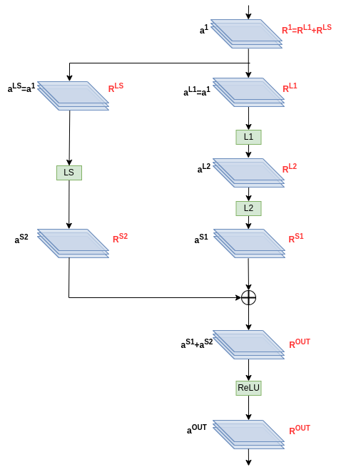
Figure 1: Illustration of residual block. Neural network layers are indicated in green, black text indicates the signal, while red text shows the corresponding LRP relevance.

Following the standard LRP procedure for shortcut connections[4]^,[10], the residual block input LRP relevance is the sum of the relevances obtained at the inputs of the principal and the shortcut path ($\bm{R}^{1}=\bm{R}^{LS}+\bm{R}^{L1}$). Moreover, the LRP relevance at the output of the summation junction ($\bm{R}^{OUT}=[R_{j}^{OUT}]$) is proportionally distributed for the two junction’s inputs[10] ($\bm{R}^{S1}=[R_{j}^{S1}]$, and $\bm{R}^{S2}=[R_{j}^{S2}]$). Consider that the summation junction sums $\bm{a}^{S1}+\bm{a}^{S2}=[a_{j}^{S1}+a_{j}^{S2}]$. For LRP-$\epsilon$ we have:

$$R_{j}^{S1}=\frac{a_{j}^{S1}}{a_{j}^{S1}+a_{j}^{S2}+\epsilon\textrm{sign}(a_{j}^{S1}+a_{j}^{S2})}R_{j}^{OUT}$$ (16)

$$R_{j}^{S2}=\frac{a_{j}^{S2}}{a_{j}^{S1}+a_{j}^{S2}+\epsilon\textrm{sign}(a_{j}^{S1}+a_{j}^{S2})}R_{j}^{OUT}$$ (17)

For LRP-$z^{+}$ (Dual ISNet) we utilize:

$$R_{j}^{S1}=\frac{max(a_{j}^{S1},0)}{max(a_{j}^{S1},0)+max(a_{j}^{S2},0)+\epsilon}R_{j}^{OUT}$$ (18)

$$R_{j}^{S2}=\frac{max(a_{j}^{S2},0)}{max(a_{j}^{S1},0)+max(a_{j}^{S2},0)+\epsilon}R_{j}^{OUT}$$ (19)

2.8 LRP Flex: a Simple, Fast and Model Agnostic Implementation of LRP

Layer-wise Relevance Propagation can explain virtually any DNN architecture[10]. However, specific coding is normally required for each network architecture. Moreover, LRP libraries are commonly large and complex, especially when they implement LRP for multiple DNN architectures. For example, the LRP Block is the PyTorch LRP implementation introduced in the original ISNet study[4], and improved in this work; to implement the rules LRP-$\varepsilon$ and LRP-z^B for the DenseNet, VGG and simple sequential networks, the LRP block utilized about 2000 lines of code. Currently, with the inclusion of the LRP-z⁺ rule and the LRP implementations for ResNets, the block has about 4000 lines.

Here, we introduce LRP Flex, an implementation of LRP-$\varepsilon$ for deep neural networks utilizing only ReLU nonlinearities in their hidden layers. It has some key advantages: first, it is exceedingly simple, requiring significantly less code lines than standard LRP implementations (e.g., the LRP Flex PyTorch code is about 10 times shorter than the LRP Block code); second, LRP Flex is model agnostic, being readily applicable to new DNN architectures, and not requiring the user to spend time writing architecture-specific code; third, LRP Flex is fast, taking advantage of highly optimized backpropagation engines available in deep learning libraries. LRP Flex can be employed to rapidly implement the original ISNet, the Stochastic ISNet, and the Selective ISNet. Furthermore, it is a practical and fast technique to explain DNN’s decisions with LRP. We explain the procedure below. It is based on an equivalent reformulation of the LRP relevance backpropagation procedure, which is explained and justified in Appendix A.

1. Initialization: modify the gradient backpropagation procedure for all ReLU functions in the neural network. In PyTorch, backward hooks can perform such alteration. Deactivate the modification when not creating LRP heatmaps. Consider that the tensor $\mathbf{G^{out}}$ (with elements $G^{out}_{k}$) is the back-propagated quantity referring to the output of a ReLU function, $\mathbf{a^{out}}$ (with elements $a^{out}_{k}$). The equation below defines the modified backpropagation rule for the ReLU. It back-propagates $\mathbf{G^{out}}$ to the input of the ReLU function, producing $\mathbf{G^{in}}$ (with elements $G^{in}_{j}$). In the equation, $\varepsilon$ is the small positive $\varepsilon$ hyper-parameter in LRP-$\varepsilon$ (e.g., 0.01).
   $G_{k}^{in}=A(a_{k}^{out})G_{k}^{out}\\ \mbox{where: }A(a_{k}^{out})=\frac{a_{k}^{out}}{a_{k}^{out}+\varepsilon}$

2. Forward pass: run the neural network and store the outputs of its ReLU functions (e.g., using forward hooks in PyTorch).

3. Modified backward pass: to explain the DNN confidence in class c, request the automatic backpropagation engine in the deep learning library (e.g., PyTorch) to calculate the gradient of the DNN class c score (logit $y_{c}$) with respect to the network’s input ($\mathbf{X}$). However, use the modified backward procedure in all ReLU functions (Step 1). Accordingly, the resulting tensor ($\mathbf{G^{0}}$) will not match the actual input gradient ($\mathbf{G^{0}}\neq\nabla_{\mathbf{X}}y_{c}$).
   To create more class-selective LRP heatmaps, request the gradient of $\tilde{\eta_{c}}$ instead of $y_{c}$ (the Selective ISNet backpropagates $\tilde{\eta_{c}}$, while the original and Stochastic ISNets backpropagate logits). $\tilde{\eta_{c}}$ is defined in the equation below, where $P_{c}$ is the estimated probability for class c (a softmax output) and $\mu$ is a positive constant hyper-parameter (e.g., 0.1), which makes $\tilde{\eta_{c}}$ bounded.
   $\tilde{\eta_{c}}=\ln(P_{c}+\mu)-\ln(1-P_{c}+\mu)$

4. Element-wise multiplication: to obtain the final LRP-$\varepsilon$ heatmap ($\mathbf{R^{0}}$), element-wise multiply the back-propagated quantity ($\mathbf{G^{0}}$) and the DNN input ($\mathbf{X}$).
   $\mathbf{R^{0}}=\mathbf{G^{0}}\odot\mathbf{X}$

The LRP Flex algorithm considers only the LRP-$\varepsilon$ rule. However, it can be easily expanded to use other rules in specific DNN layers. For example, the ISNet utilizes LRP-z^B for the first network layer. To use this special first layer rule with LRP Flex, we must stop the backpropagation of G at the output of the first DNN layer. I.e., we change Step 3 of the procedure above: we now request the backpropagation engine for the gradient of the DNN logit (or of $\tilde{\eta_{c}}$) with respect to the output of the first DNN layer ($\mathbf{a^{1}}$, the output of the network’s first ReLU), and use the modified ReLU backpropagation rule (Step 1). Step 4 is also changed: we element-wise multiply the tensor obtained in the modified Step 3, $\mathbf{G^{1}}$, with the output of the first DNN layer, $\mathbf{a^{1}}$, obtaining the LRP-$\varepsilon$ relevance at the output of the first DNN layer ($\mathbf{R^{1}}=\mathbf{G^{1}}\odot\mathbf{a^{1}}$, following Equation 20). Finally, the relevance $\mathbf{R^{1}}$ can be back-propagated trough the first DNN layer according to the standard LRP-z^B rule[10] (e.g., following the implementation in the LRP Block[4]), generating the LRP heatmap ($\mathbf{R^{0}}$). As noted in the original ISNet study[4], the use of LRP-z^B is not mandatory for training an ISNet, nor is it necessary for the Faster ISNet.

2.9 Benchmark DNNs

For both the COVID-19 detection and the biased MNIST classification tasks, we compare the Faster ISNet formulations to standard classifiers, which employ the same architecture as the ISNet classifier (ResNet18 for MNIST and DenseNet121 for COVID-19 detection). The comparison will allow us to assess the effect of the ISNet’s LRP optimization on shortcut learning, generalization capacity and attention to background bias. Moreover, we also compare the new models to the original ISNet[4] in all applications. The low image resolution of MNIST is not detrimental to input gradients and Gradient*Input explanations. Therefore, in the application we also compare the Faster ISNet to the ISNet Softmax Grad*Input (Section 2.5) and the Right for the Right Reasons neural network[12] (RRR). Both also utilize the ResNet18 backbone. RRR is based on the optimization of input gradients during training. It uses a square loss to minimize the background region of the gradients. This region is defined according to segmentation masks[12]. Here, input gradients are the gradients of the summed log probabilities for all possible classes, with respect to the DNN input[12]. As the ISNet, RRR’s objective is to produce classifiers whose decisions ignore background features.

This study utilizes the same COVID-19 detection dataset used in the original ISNet paper[4]. Therefore, we can directly compare the Faster ISNet performance to multiple state-of-the-art neural network architectures that control classifier attention, which were already tested in the original ISNet report[4]. They are: the original ISNet[4], a standard segmentation-classification pipeline[4], multi-task DNNs[31], attention-gated neural networks (AG-Sononet)[18], Guided Attention Inference Networks (GAIN)[15], RRR[12], and vision transformer (ViT-B/16)[17]. Because MNIST images and the corresponding late feature maps are exceedingly small, most of the baseline models were not adequate for MNIST classification. However, although we do not train the segmentation-classification pipeline on MNIST, we train and test a classifier (ResNet18) on the unbiased (standard) MNIST dataset, simulating the classifier performance on perfectly segmented images. More details about implementations, hyper-parameters, and training procedures for the alternative deep neural networks on the COVID-19 classification dataset can be found in the original ISNet paper[4]. Below, we summarize these different state-of-the-art methodologies[4].

First, we compare the ISNet to a standard technique used for datasets containing background bias, the segmentation-classification pipeline: a deep semantic segmenter identifies the image foreground (e.g., lungs), the segmenter output is thresholded and used to substitute the image’s background by zeros, and finally a deep classifier classifies the segmented image. In the ISNet original study, this segmentation-classification pipeline was the only alternative model that could also be insensitive to the presence of background bias[4]. However, the network was still surpassed by the ISNet in all experiments performed in the study[4]. The pipeline represents a much larger and slower model during run-time, due to the utilization of two deep neural networks. The segmenter in the model is a standard U-Net[32], and the classifier a DenseNet121[19], matching the ISNet classifier. We notice that the U-Net is a semantic segmenter especially designed for biomedical images[32], composed of a contracting signal path, followed by an expanding path. The paths are connected by multiple skip connections. The U-Net is pretrained on the COVID-19 dataset, using its segmentation targets[4]. Afterward, the segmenter parameters are frozen, and the classifier is trained with the same database.

The ISNet’s background relevance minimization can be seen as a spatial attention mechanism (explanation-based), because it represents a technique designed to control a classifier’s attention over the input space[4]. Accordingly, we compare the model to a state-of-the-art attention mechanism, the AG-Sononet[18]. Attention gated networks were designed to substitute the aforementioned pipeline of segmentation-classification, especially for biomedical images[18]. Its objective is to increase classifier focus on important image features, and reduce attention to background clutter (features uncorrelated to the sample class). The AG-Sononet introduced attention gates, a structure that performs the element-wise multiplication of a convolutional layer’s feature map and attention coefficients. The coefficients are defined as a function of two tensors: the gated layer’s feature map, and the output of a late convolutional layer (e.g., the last). The AG-Sononet is based on a VGG-16 classifier, and the considered implementation[4] followed the AG-Sononet official code[18]. The model exemplifies the paradigm of not using segmentation targets to guide the classifier attention. Like the AG-Sononet, most spatial attention mechanisms rely solely on the classification labels and the classification loss to teach the DNN what features are relevant in an image[33]. The AG-Sononet architecture presents minimal computational overhead in relation to standard classifiers, and it was successfully used to avoid classifier focus on background clutter. The model was evaluated on fetal ultrasounds, which represent noisy and hard to interpret images[18].

The Vision Transformer[17] is a popular neural network architecture, which is built upon an attention mechanism, the transformer’s self-attention. Like the AG-Sononet, it does not learn from segmentation targets. The Transformer was highly successful in natural language processing (NLP), its attention mechanism relates diverse positions in an input sequence, generating a new representation of the sequence. It is also employed as a benchmark in the COVID-19 detection task[4]. Specifically, the implemented network is the base model ViT-B/16[17], because, with respect to alternative variants, its number of parameters is closer to the other benchmark networks[4].

As an additional benchmark, we consider a multi-task DNN simultaneously performing semantic segmentation and classification[31]. Such networks begin as a shared sequence of convolutional layers, which fork into two independent paths, the classification head and the segmentation head. The first outputs classification scores, while the second produces semantic segmentation outputs. To optimize the entire network, the model utilizes a linear combination of a classification loss (employing classification targets) and a segmentation loss (using segmentation masks). The objective of the segmentation loss is simply the creation of semantic segmentation outputs. Thus, it is vastly different from the ISNet’s heatmap loss, whose objective is the control of what input features influence the classification scores. Moreover, the segmentation outputs in the multi-task network are produced by an independent structure, the segmentation head. They are not explanations of the classifier scores, nor necessarily related to the classifier’s behavior[4], like the LRP heatmaps optimized by the ISNet.

Nevertheless, the original ISNet work[4] tested if the multi-task network can be resistant to background bias, because studies suggested that the segmentation task can help the classifier ignore irrelevant background clutter, improving accuracy[34]^,[35]. Example of noisy and cluttered images, where multi-task learning improved classification, were capsule endoscopy pictures[34] and breast ultrasound[35]. The multi-task DNN implemented in the original ISNet study[4] is based on the U-Net architecture, with an additional classification head attached to the network bottleneck feature representation (end of the U-Net contracting path). The U-Net contracting path is based on the VGG-16 architecture. Thus, the classification head follows the VGG-16 last layers[30], consisting in average pooling (outputting 7x7 sized feature maps), followed by three dense layers, the first two with 4096 neurons. The classification head utilizes 50% dropout layers after the first two dense layers, and we included batch normalization before each ReLU activation in the U-Net body to improve training convergence[4].

Finally, the last benchmark DNN in COVID-19 detection is the Guided Attention Inference Network (GAIN)[15]. The model was proposed to create a classifier whose Grad-CAM heatmaps more completely indicate the objects in the images, serving as priors for weakly supervised semantic segmentation[15]. As an additional benefit, GAIN’s authors claim that the architecture can reduce classifier attention to background bias[15]. Like the ISNet, GAIN directly optimizes explanation heatmaps. However, it penalizes Grad-CAM heatmaps instead of LRP maps. Refer to the original ISNet study[4] for a theoretical comparison between the two methodologies, and for an analysis of the LRP optimization advantages. Besides the standard classification loss (e.g., cross-entropy), two loss functions penalize the Grad-CAM explanations, the attention mining loss and the external supervision loss[14]. The network classifies an image, produces its Grad-CAM heatmaps for the ground-truth classes, and utilizes the explanations to remove the high attention region from the input image. When multiple classes are present, multiple heatmaps and altered images are generated. The new figures are classified again, and the attention mining loss is defined as the mean value of new ground-truth classes’ logits[14]. The loss minimization prompts the neural network to pay attention to all input image regions that are correlated to the sample labels, extending the Grad-CAM attention. The external supervision loss is the mean squared error between the Grad-CAM maps for the ground-truth classes and the respective segmentation targets. It is presented as an optional loss, which is important for resistance to background attention[15]. Thus, to maximize bias resistance, the GAIN implementation in the original ISNet paper[4] utilizes the external supervision loss for all training images. GAIN with the external supervision loss can also be called extended GAIN[15]. The classifier chosen as backbone for GAIN was the DenseNet121, matching the ISNet classifier[15]. GAIN’s Grad-CAM considers the last convolutional feature map in the DNN, the standard choice for GAIN[15]. Latter heatmaps contain higher-level semantics[14], and allow the utilization of more DNN layers (and flexibility) to satisfy the GAIN losses.

2.10 Data Processing

MNIST images were loaded in grayscale, standardized with pixel values between 0 and 1, and fed to the neural networks. In MNIST, we do not employ data augmentation, maximizing the synthetic bias influence over the classifier. Standard augmentation procedures (e.g., rotations and translations) can partially or totally remove the bias from the network input. The MNIST images’ size is 28x28. The grayscale images were repeated in 3 channels to match the ResNet18 input shape. Although single-channel figures could be used, without profound changes in the classifier architecture they would provide minimal performance advantages over the standard 3-channel images.

The X-rays were processed and augmented following the procedures in the original ISNet study[4], allowing direct comparisons to the neural networks trained in the past work. We loaded the images in grayscale, applied histogram equalization, resized them to 224x224 pixels, repeated the images in three channels, and performed data augmentation. Test images were made square by adding black rectangles to their borders before resizing. The strategy prevents any bias related to aspect ratio from affecting the test results. By not employing the bars in training images, we do not allow neural networks to learn how to analyze the rectangles (especially the models without segmentation). Data augmentation was used only for training images, and it consisted in random translation (up to 28 pixels up/down and left/right), random rotation (from -40 to 40 degrees), and random flipping (50% probability). Data augmentation was employed to avoid overfitting, and to make the DNN more resistant to the natural occurrence of the operations (rotations, translations and flipping). Moreover, it allows the ISNet evaluation under a standard data augmentation protocol.

2.11 Training Procedure

For a fairer comparison, we trained all neural networks with similar procedures and hyper-parameters. All models were implemented in PyTorch and trained on an NVIDIA RTX 3080 or an NVIDIA Tesla V100. All networks’ trainable parameters were randomly initialized, because the utilization of pretrained models could reduce the generality of the conclusions drawn from a shortcut learning study (refer to the original ISNet article for a detailed explanation[4]). Gradient norm clipping (with norm 1) was employed to improve the training procedure’s stability. Weight decay was not utilized and the LRP-$\varepsilon$ $\varepsilon$ hyper-parameter was set to 0.01, like in the original ISNet study[4].

For MNIST we utilized the stochastic gradient descend (SGD) optimizer, with momentum of 0.9, mini-batches of 128 samples, learning rate of 0.01 (or 0.001 for the Stochastic ISNet and ISNet Softmax Grad*Input), and 100 epochs. Hold-out validation was utilized to choose the best neural network, considering synthetic bias in the validation data. All ISNet variations employed the loss hyper-parameters of: P=0.9, d=0.9, and $w_{1}=w_{2}=1$. For RRR, we set the Right Reasons loss’ weight[12] to 1000. Training the neural networks with synthetically biased images, the loss hyper-parameters were chosen to maximize accuracy in a version of the validation dataset with the synthetic bias removed.

For COVID-19 detection, we followed the training procedure in the original ISNet paper[4], as it guided the optimization of all benchmark DNNs we compared the Faster ISNet to. Specifically, we trained for 48 epochs, with hold-out validation, learning rate of 0.001, stochastic gradient descend, momentum of 0.99, and mini-batches of 16 samples. All Faster ISNets employed the loss hyper-parameter d of 0.999, $w_{1}=1$ and $w_{2}=3$. The loss parameter P was set to 0.8 in the Selective and Dual ISNets, 0.7 in the Stochastic ISNet, and 0.1 in the ISNet Softmax Grad*Input. The RRR Right Reasons loss’ weight[12] was $10^{6}$, and GAIN’s[15] loss terms’ weights were: 1 for the classification loss, 1 for attention mining, and 10 for the external supervision[4]. Hyper-parameters were chosen according to a search procedure that does not require access to o.o.d. data. It is described in detail in the first ISNet study[4].

2.12 Statistical Analysis of Performance Metrics

Being a contemporary and critical application, it is important to report uncertainty in COVID-19 detection. For the task, we present the networks’ precision, recall, sensitivity, and F1-Score. The metrics are derived from the neural networks’ confusion matrix. To provide their interval estimates we employ Bayesian evaluation. We resort to the same Bayesian model[36] that was used in the original ISNet study[4]. It was proposed to take a confusion matrix and output posterior estimates of precision, recall, and F1-Score. Moreover, it was expanded in a subsequent study[5] to also create interval estimates for specificity. Posteriors were estimated with Markov chain Monte Carlo (MCMC), implemented with the Python library PyMC3[37]. We utilized the No-U-Turn Sampler[38], using 4 chains and 110000 samples, being the first 10000 for tuning. The estimator’s Monte Carlo error remained below 10^-4 for all metrics. We employed the same priors as the Bayesian model creators[36]. To calculate the macro-average ROC AUC (area under the receiver operating characteristic curve), we utilized a pair-wise approach[39] developed for multi-class single-label problems (such as COVID-19 classification). There is no established methodology to calculate interval estimated for this metric, and its authors suggested bootstrapping[39], a technique that would not be feasible with the deep models and cross-dataset evaluation used in this study.

3 Results

Here, we report and analyze the neural networks’ performance and resistance to background bias and shortcut learning in the biased MNIST and COVID-19 data.

3.1 Datasets

This study performed experiments on two datasets, the synthetically biased MNIST database, and the COVID-19 dataset[4].

3.1.1 Biased MNIST

The biased MNIST dataset samples were drawn from the original MNIST database[22], a balanced dataset of hand-written digits (from 0 to 9), consisting in 60000 28x28 grayscale images. We consider the same test partition as the original database[22] (10000 images), and randomly split the remaining 50000 images, selecting 80% for training and 20% for hold-out validation.

We added synthetic bias to all training data. The MNIST images’ background is black (0). Thus, to create a simple and attention grabbing background bias, we set to white the (c+1)^th pixel, from left to right, in the image’s top row. E.g., for an image displaying the digit 0, we set the pixel in the top left corner to 1 (white). Figure 2 provides an example of a training image. Due to its simplicity, it should be much easier for a classifier to produce decision rules based on the bias, instead of analyzing the more complex features of the hand-written digit. Therefore, we designed the dataset to be strongly prone to shortcut learning.

Figure 2: Example of training sample from biased MNIST. The figure represents the digit 1. Accordingly, the second pixel (from left to right) in the image’s top row was set to 1, representing background bias.

We also add the artificial bias to the hold-out validation dataset, which will be used to select the best performing DNN iteration after training. However, we employ an unbiased version of the validation set to tune the ISNet loss hyper-parameters P and d. Finally, we have three different test databases: the i.i.d. set has the same artificial bias as the training data; the o.o.d. dataset does not have any artificial bias; the deceiving bias dataset has synthetic bias, but the correspondence between the ground-truth class and the highlighted background pixel is changed. In the deceiving bias dataset, we highlight the (c+2)^th top pixel for the digit c, except for the digit 9, where we highlight the first pixel (top left corner). A classifier suffering from shortcut learning should perform well on the i.i.d. test, lose accuracy on the o.o.d. test, and lose even more performance on the deceiving evaluation.

3.1.2 COVID-19 X-ray Classification

Unlike MNIST, X-rays represent high-resolution data (224x224 in our dataset), and exemplify a natural occurrence of background bias. It is common for large X-ray databases portraying a disease not to have enough samples representing other conditions of interest, or to have such samples drawn from diverse hospitals. To train reliable deep classifiers, large databases adequately representing all conditions of interest are important. When such data is not available from a single source (or from a set of sources with similar class distributions), studies normally employ mixed source databases, where samples representing different categories (e.g., diseases) were drawn from distinct locations (hospitals). Each source is correlated to particular background characteristics (e.g., specific text in the X-ray background[40]). Since, in mixed datasets, the different sources represent different classes, their distinct background features become correlated to the image labels, constituting background bias and causing shortcut learning[3]^,[2]^,[4].

Dataset mixing is common in COVID-19 classification[41]. The COVID-19 dataset from the original ISNet study[4] purposefully exemplifies such scenario. Each class (COVID-19, pneumonia and healthy) was extracted from a different dataset. These datasets originated from diverse sets of hospitals and cities. They were chosen due to their large size, high quality and adequate documentation. Hold-out validation images were randomly selected, and they share sources with the training images. Hold-out validation represents 25% of the non-test images. There is no patient with X-rays in the training and validation splits. Importantly, to estimate generalization to real-world data, the dataset test samples were not randomly drawn from the same sources providing the training and hold-out validation data. Instead, we utilize an out-of-distribution test dataset. I.e., all test X-rays were drawn from hospitals and cities never utilized to gather training or hold-out validation data. For a detailed description of the dataset, including information about data acquisition time and methodology, disease severity, exclusion criteria, equipment used, data format, and labeling scheme, please refer to the study presenting the database[4]. In the remaining of this section we briefly summarize it.

All images in the dataset are frontal X-rays from adult patients, collected from open sources. Specifically, the COVID-19 training and hold-out validation data consists in 4644 positive samples from the Brixia COVID-19 X-ray dataset[6], being all images that show visible (Brixia score higher than 0) signs of the disease. All images come from the same hospital, ASST Spedali Civili di Brescia, Brescia, Italy. The database is one of the largest COVID-19 data collections to date, and it was created to simulate a real clinical scenario: the images represent all triage and patient monitoring (in sub-intensive and intensive care units) X-rays collected between March 4th and April 4th, 2020, reflecting real-world variability[6]. Training and validation X-ray images showing the healthy (4644) and pneumonia (4644) conditions were randomly extracted from the CheXPert database, one of the largest and most well-known chest X-ray datasets[42]. This data collection originated in the Stanford University Hospital, California, United States of America[42]. COVID-19 images were labeled by radiologists on-shift[6]. Meanwhile, the other classes were labeled by natural language processing, according to radiological reports[42].

The external (o.o.d.) test dataset has 1515 COVID-19 X-rays, extracted from the BIMCV COVID-19+ (iterations 1+2)[43] database. The data collection is also among the largest open COVID-19 X-ray datasets. It was produced between February 16th and June 8th, 2020. Samples were obtained from the health departments in the Valencian healthcare system, Spain, which involves multiple hospitals, mostly in the provinces of Alicante and Castellón[43]. Furthermore, our o.o.d. test data contains 1295 test X-rays representing the pneumonia class, which were gathered from the ChestX-ray14 database[44]. Like CheXPert, the data collection is also one of the largest and most well known chest X-ray databases. It was created in the National Institutes of Health Clinical Center, Bethesda, United States of America. Finally, the healthy class X-rays were extracted from a database assembled in Montgomery County, Maryland, USA (80 images), and Shenzhen, China (326 images)[45]. They were gathered from the Montgomery County’s Tuberculosis screening program, in collaboration with the local Department of Health and Human Services, and from Shenzhen No.3 People’s Hospital, Guangdong Medical College (Shenzhen, China). All the healthy class samples were manually labeled by radiologists[45]. COVID-19 images were labeled by radiologists and correspond to patients with at least one positive COVID-19 PCR or immunological test in the BIMCV COVID-19+ data acquisition time period (February 16th to June 8th, 2020)[43]. Meanwhile, the pneumonia labels were assigned by natural language processing, according to radiological reports[44].

3.2 Synthetically Biased MNIST

Table 1 reports the DNNs’ results on the biased MNIST application according to overall accuracy, as is the standard for the MNIST dataset[22]. We trained the neural networks with images including the synthetic bias (white background pixels, correlated to the image classes), and evaluated them on the official MNIST test database. There are three different versions of the test set: i.i.d., which also contains the artificial bias, o.o.d., corresponding to the original MNIST test images, and deceiving bias, where the biasing pixel that represented one class during training now represents another.

Table 1: Test results for the neural networks trained on MNIST with synthetic background bias. The i.i.d. test data contains the same bias as the training dataset, the o.o.d. test database has no background bias, and the deceiving bias test has bias designed to fool the classifiers

Neural Network	Test Accuracy (i.i.d.)	Test Accuracy (o.o.d.)	Test Accuracy (Deceiving Bias)
ResNet18	100%	51.33%	0.85%
Original ISNet	97.76%	97.76%	97.76%
Selective ISNet	98.73%	98.73%	98.73%
Dual ISNet	98.62%	98.62%	98.63%
Stochastic ISNet	97.76%	97.76%	97.75%
ISNet Softmax Grad*Input	96.94%	96.94%	96.94%
RRR	97.75%	97.46%	97.45%
ResNet18 Trained without Synthetic Bias	-	99.16%	-

First, the results of a standard classifier (the ResNet18) show that the tendency for shortcut learning is extreme in this dataset. The model behaved like a perfect classifier when the synthetic background bias was present in the test data, achieving 100% accuracy (i.i.d. test). However, the bias strongly reduced the neural network capacity to analyze the images’ foreground features (the digits). Consequently, when the bias was removed from the test data (o.o.d. test), the model’s accuracy dropped to 51.33%. For reference, a ResNet18 trained on the MNIST dataset without the synthetic bias achieved 99.16% test accuracy. Finally, the deceiving bias was capable of fooling the ResNet18 (trained with synthetic bias) almost every time, reducing its accuracy to 0.85%. Therefore, we observe a case of extreme shortcut learning, where the influence of background bias on the classifier’s decisions is paramount.

Moreover, Table 1 shows that in the biased MNIST classification task all LRP ISNet variants (original, selective, dual and stochastic) were resistant to the influence of background bias, with virtually no accuracy change across the i.i.d., o.o.d., and deceiving bias evaluations. Furthermore, they were accurate, with accuracies only 0.43 to 1.4% behind the results for a network trained on a dataset without the artificial bias. The ISNet Softmax Grad*Input was also resistant to background bias, but its accuracy was surpassed by the other ISNets. Finally, RRR presented a small accuracy reduction when the synthetic bias was removed from the test data (0.29% drop), unlike the ISNets. By increasing the RRR’s right reasons loss weight ($\lambda_{1}$), from 1000 to 10000, bias resistance increased, but overall accuracy decreased. With $\lambda_{1}=10000$, RRR achieved accuracies of 96.13%, 96.02% and 96.03%, in the i.i.d., o.o.d. and deceiving evaluation, respectively.

3.3 COVID-19 Detection in Chest X-Rays

COVID-19 detection with mixed datasets is a task known for background bias and the consequent tendency for shortcut learning[4]^,[2]^,[3]. Shortcut learning reduces the neural networks’ generalization capacity, making them lose accuracy on out-of-distribution (o.o.d.) data. Therefore, reductions in background attention and shortcut learning allow neural networks to perform better on the o.o.d. COVID-19 test dataset, which considers only hospitals that did not contribute to the training data. Table 2 displays the o.o.d. test F1-Scores for all neural networks proposed and implemented in this study (Stochastic ISNet, Selective ISNet, Dual ISNet and ISNet Softmax Grad*Input). Moreover, it also portrays the performance scores for multiple alternative DNNs, trained in the study presenting the original ISNet[4]. Allowing a fairer comparison, the past study employed the same dataset, training procedure, data augmentation, and image processing techniques as the current study. The alternative models are described in Section 2.9. Except for RRR, the remaining benchmark models were not implemented for the MNIST classification task, due to the small resolution of the MNIST images.

Table 2: Out-of-distribution test performances for neural networks in COVID-19 detection (evaluation on X-rays from hospitals not seen during training)

Neural Network	Normal F1-Score	Pneumonia F1-Score	COVID-19 F1-Score	Macro-average F1-Score
Selective ISNet	0.493 +/-0.021, [0.453,0.534]	0.822 +/-0.008, [0.806,0.839]	0.888 +/-0.006, [0.876,0.9]	0.734 +/-0.009, [0.717,0.752]
Dual ISNet	0.529 +/-0.019, [0.492,0.566]	0.768 +/-0.01, [0.75,0.787]	0.921 +/-0.005, [0.911,0.931]	0.739 +/-0.009, [0.723,0.756]
Stochastic ISNet	0.505 +/-0.021, [0.465,0.545]	0.799 +/-0.009, [0.781,0.817]	0.836 +/-0.007, [0.822,0.85]	0.714 +/-0.009, [0.696,0.731]
ISNet Softmax Grad*Input	0.251 +/-0.014, [0.224,0.278]	0.25 +/-0.015, [0.221,0.28]	0.867 +/-0.006, [0.855,0.88]	0.456 +/-0.008, [0.441,0.471]
Original ISNet[4]	0.555 +/-0.022, [0.512,0.597]	0.858 +/-0.007, [0.844,0.871]	0.907 +/-0.006, [0.896,0.918]	0.773 +/-0.009, [0.755,0.791]
DenseNet121[4]	0.444 +/-0.02, [0.403,0.482]	0.434 +/-0.015, [0.405,0.463]	0.76 +/-0.008, [0.744,0.775]	0.546 +/-0.01, [0.527,0.565]
U-Net+DenseNet121[4]	0.571 +/-0.018, [0.535,0.607]	0.586 +/-0.013, [0.561,0.611]	0.776 +/-0.008, [0.76,0.792]	0.645 +/-0.009, [0.626,0.663]
Multi-task U-Net[4]	0.419 +/-0.025, [0.369,0.469]	0.119 +/-0.011, [0.098,0.14]	0.585 +/-0.009, [0.566,0.602]	0.374 +/-0.01, [0.355,0.394]
AG-Sononet[4]	0.124 +/-0.015, [0.096,0.153]	0.284 +/-0.015, [0.255,0.312]	0.659 +/-0.009, [0.641,0.676]	0.356 +/-0.008, [0.34,0.372]
Extended GAIN[4]	0.203 +/-0.019, [0.166,0.24]	0.485 +/-0.013, [0.46,0.511]	0.711 +/-0.009, [0.693,0.728]	0.466 +/-0.009, [0.449,0.485]
RRR[4]	0.36 +/-0.018, [0.325,0.394]	0.552 +/-0.013, [0.526,0.577]	0.737 +/-0.009, [0.72,0.755]	0.55 +/-0.009, [0.532,0.568]
Vision Transformer[4]	0.382 +/-0.017, [0.348,0.415]	0.474 +/-0.013, [0.448,0.499]	0.525 +/-0.011, [0.503,0.548]	0.46 +/-0.009, [0.443,0.478]

Scores in the table are expressed as mean +/-std, [95% HDI]. Mean refers to the metric’s mean value, considering its probability distribution, and std refers to its standard deviation. The 95% high density interval (HDI) is an interval containing 95% of the metric’s probability mass. Moreover, any point inside the interval has a higher probability density than any point outside of the interval. Please refer to Section 2.12 for more details about our statistical analysis.

We observe that the LRP-based ISNets (Original ISNet, Stochastic ISNet, Selective ISNet, and Dual ISNet) significantly surpassed all benchmark models. These results demonstrate the advantages of LRP optimization over alternative methodologies, such as attention mechanisms that do not consider segmentation targets, multi-task DNNs, and the optimization of Grad-CAM, input gradients and Grad*Input. Therefore, the empirical results corroborate with the analysis in the original ISNet paper[4], which theoretically explained the process of LRP optimization, and fundamentally compared it to multiple state-of-the-art methodologies designed to avoid background attention.

The original ISNet[4] has a small average F1-Score advantage over the Faster ISNets. Therefore, the new models present a trade-off, exchanging a bit of accuracy for faster training. For a critical application with a small number of classes, the trade-off may not be worth it. However, depending on the number of categories in the classification task, the Faster ISNet can drastically reduce training time, and training the original network may not even be viable (Section 3.4).

The models optimizing input gradients and Gradient*Input (i.e., RRR and the ISNet Softmax Grad*Input, respectively) could almost match the LRP-based ISNets on the MNIST classification task, but they were significantly surpassed in COVID-19 classification. In relation to MNIST classification, COVID-19 detection considers higher resolution data (224x224 versus 28x28) and deeper neural networks (121 layers in the DenseNet121 backbone, against 18 layers in the ResNet18). The new setting is challenging for ISNet Softmax Grad*Input and RRR, as the explanations optimized by the models become noisy for deep architectures analyzing high-dimensional data[27]. The noisiness harms the models’ optimization procedure[4]. In relation to RRR[12], the ISNet Softmax Grad*Input has a more restrictive loss function penalizing the heatmaps[4] (Section 2.3). It could not adequately converge in COVID-19 detection, remaining high and unstable. Meanwhile, RRR achieved a low heatmap loss. However, the loss was low due to an overall reduction of the input gradient magnitude, not due to a model that is paying little attention to the images’ backgrounds. Please refer to the original ISNet study[4] for an in-depth explanation of this phenomenon.

The first ISNet study[4] implemented the ISNet Grad*Input, an ablation experiment where the original ISNet LRP heatmaps were substituted by Gradient*Input explanations. Like the ISNet Grad*Input, the ISNet Softmax Grad*Input was also unstable with very deep classifiers, resulting in its low performance in Table 2[4]. Thus, the experiments with RRR[4], the ISNet Grad*Input[4], and the ISNet Softmax Grad*Input demonstrate that, in relation to input gradients and Gradient*Input, LRP optimization is more stable and leads to higher accuracy and resistance to background bias, especially with deeper backbones. Moreover, the large performance gap between the LRP-based ISNets and GAIN[15] (Table 2) demonstrates the advantages of LRP optimization over Grad-CAM optimization. Please refer to the original ISNet study[4] for a detailed theoretical justification of LRP optimization’s empirically verified advantages over the optimization of Grad-CAM, input gradients, and Gradient*Input.

The results in Table 2 are in line with past studies that classified COVID-19 X-rays and employed o.o.d. evaluation (i.e., testing with X-rays from hospitals that did not contribute to the training data). For example, the DenseNet121 in Table 2 achieved 0.808 ROC AUC[4] (area under the receiver operating characteristic curve, calculated with a pair-wise technique[39]). The value falls within the confidence interval reported by a past study[3], which trained a DenseNet121 and tested it with an o.o.d. dataset, obtaining 0.786 +/-0.025 ROC AUC. Moreover, another work[5] also utilized o.o.d. evaluation and a DenseNet121 classifier, but they employed a deep lung segmenter before the classification procedure. Its model achieved maF1 of 0.754, with 95% HDI of [0.687,0.82]. We observe that all LRP-based ISNets maF1 scores’ HDIs (Table 2) fit inside their reported HDI. Thus, the results in this study align with other works that consider external validation. Conversely, many studies that employed i.i.d. evaluation for COVID-19 detection (normally, by randomly dividing a database, creating a training and a testing partition) report much higher test performances, with F1-Scores sometimes close to 100%[41]. Such large performance discrepancy is explained by shortcut learning: the problem makes the neural networks perform well on i.i.d. data, but they lose much accuracy on o.o.d. evaluation and real world data, because it does not contain the biases present in i.i.d. data. Therefore, our empirical results corroborate with multiple studies that analyzed the phenomenon of background bias and shortcut learning in COVID-19 detection[3]^,[2]^,[4]^,[46]^,[7]^,[5].

3.4 Training and Run-time Speed

The Faster ISNet and the original ISNet have the same run-time speed as a standard classifier, because the creation of LRP heatmaps is not necessary after training. E.g., any ISNet with a DenseNet121 backbone will be as fast as a standard DenseNet121 at run-time. In COVID-19 detection, the segmentation-classification pipeline (U-Net followed by DenseNet121) was the second-best performing neural network, losing for the ISNet. Moreover, in the original ISNet study[4], it was the only benchmark model that could reliably avoid the influence of synthetic background bias on the classifier’s decisions, like the ISNet. However, at run-time, the model is much slower than any ISNet variant, as it involves running two deep neural networks, instead of one. We compare the run-time ISNet with a DenseNet121[19] backbone to the pipeline composed of an U-Net[32] and the DenseNet121. We consider mixed-precision, mini-batches of 10 images (of size 224x224x3), and an NVIDIA RTX 3080. The ISNet was able to process an average of 353 samples per second, while the pipeline processed 207[4]. Without mixed-precision, the ISNet processed 298 samples per second, and the pipeline 143. Thus, the ISNet was 70 to 108% faster[4]. Moreover, the model had only 8M parameters, while the pipeline had 39M, being about 5 times larger. Therefore, the ISNet (both the original and the Faster ISNet) is a significantly faster and lighter model after training. Such efficiency is especially important for its deployment in mobile or less capable devices.

The original ISNet disadvantage is its training time. The model creates one LRP heatmap for each DNN output neuron. Thus, its training time increases approximately linearly with the number of classes in the classification problem[4]. Considering a classification problem with 3 classes, 24183 training images and 2993 validation samples, the original ISNet took about 1300 s per epoch[4]. Meanwhile, the benchmark neural networks training times were: 1500 s for GAIN, 900 s for RRR, 320 s for the segmentation-classification pipeline (and 400 s per epoch when pre-training its U-Net), 240 s for the DenseNet121, 250 s for the multi-task U-Net, 160 seconds for the vision transformer, and 60 s for the AG-Sononet[4].

The Faster ISNet advantage over the original ISNet is that its training time does not increase linearly with the number of classes in the classification task. Figure 3 compares the training time for the original and the Faster ISNets, employing a log-log plot. It displays the time for one epoch, considering 13932 images (with 80% used for training and 20% for validation), with resolution of 224x224 and 3 channels. The networks run in an NVIDIA RTX 3080 with mixed precision. We simulate 1 to 1000 classes in the classification task, by varying the number of output neurons in the networks. For realism, we set a fixed limit of GPU (graphics processing unit) memory; we selected 10 gigabytes, which is about the limit in the RTX 3080. Accordingly, the mini-batch size is always set to approximately utilize the 10 gigabytes of video memory. The original ISNet memory utilization increases while we generate LRP heatmaps in parallel, thus we reduce batch size while increasing the number of classes. When batch size reaches one, we start generating heatmaps in series, which makes the model’s training time increase linearly. In Figure 3, the original ISNet’s batch size reaches one with about 10 classes (considering 10 GB of video memory).

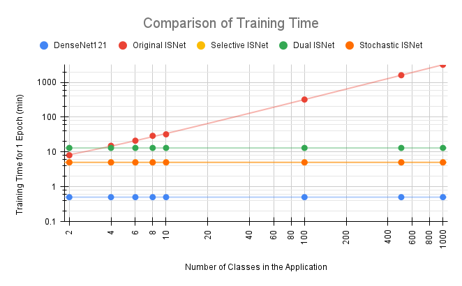
Figure 3: Training time for multiple neural networks, considering one epoch of 13932 224x224x3 images, and a varying number of categories in the classification problem.

As expected, the original ISNet training time increases approximately linearly with the number of classes in the classification task. Meanwhile, the training time for all Faster ISNet variations (Selective, Dual, and Stochastic) is independent of the number of classes, like for the standard DenseNet121. The common classifier training time was 0.5 min per epoch, the Stochastic ISNet and the Selective ISNet achieved both 5 min per epoch, and the Dual ISNet, needing two LRP heatmaps per image, required 13 minutes per epoch. The original ISNet was always slower than the Selective and Stochastic ISNets. It was faster than the Dual ISNet until about 3 classes in the classification problem, becoming increasingly slower afterward. To put the numbers in Figure 3 into perspective, it would take about 8.3 hours to train the Selective or Stochastic ISNet for 100 epochs (considering the data and hardware we used to generate Figure 3). Meanwhile, the original ISNet would require 13 hours for 2 classes, 50 hours for 10 classes, and about 220 days with 1000 classes. Its training time could be reduced with more powerful hardware and parallelism over multiple GPUs. However, such settings represent high cost and massive electrical energy consumption. Therefore, besides improving training time, the Faster ISNet expands the number of applications where LRP optimization can be feasibly implemented.

3.5 Heatmap Analysis

Figure 4 presents LRP heatmaps for biased MNIST test images (i.i.d. test). Thus, the images contain the same synthetic background bias found in training data (the white pixels in the images’ upper region). The heatmaps demonstrate that no ISNet payed attention to the bias, RRR payed minimal attention to it, while the standard classifier mostly focused on bias. Such findings corroborate with the quantitative results in Table 1, which prove that the synthetic bias had no influence over the ISNet decisions, a small influence over RRR, and major influence over the standard ResNet18.

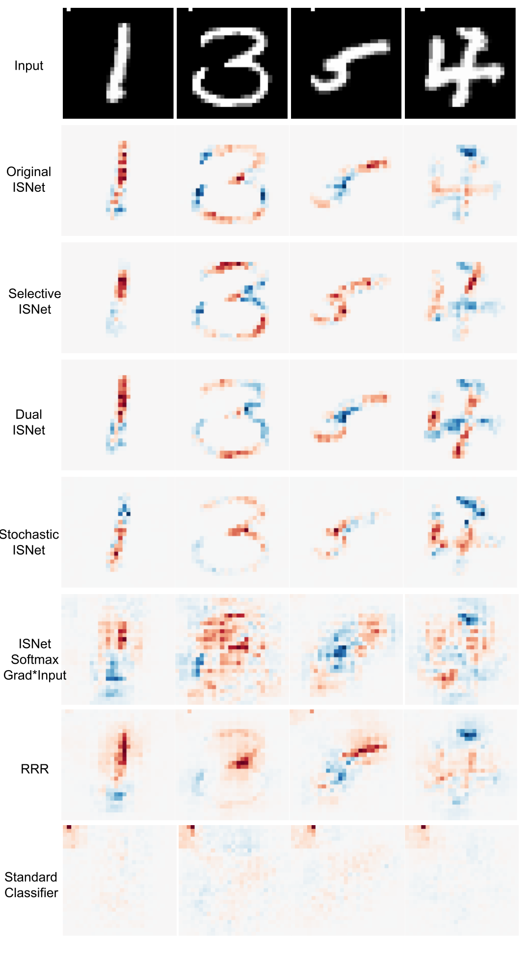
Figure 4: LRP heatmaps for the MNIST classification task. A white pixel in the images’ top left corner represents synthetic background bias. Red colors indicate areas that contributed for the DNN confidence in the images’ true class, while blue areas reduced such confidence. White regions were not important for the DNN decision.

Figure 5 portrays LRP heatmaps for the COVID-19 classification task. Heatmaps for the original ISNet and the DenseNet121 were extracted from the first ISNet study[4]. Please refer to it for heatmaps representing the remaining neural networks in Table 2 (RRR, GAIN, multi-task DNN, AG-Sononet, vision transformer, and segmentation-classification pipeline). In summary, the heatmaps in Figure 5 and in the past study[4] demonstrate that all neural networks have clear attention to background bias, except for the segmentation-classification pipeline and the LRP-based ISNets (original, Selective, Dual, and Stochastic ISNet). Here, background means all X-ray regions outside of the lungs. An example of background bias is a mark over the right shoulder in the pneumonia X-ray in Figure 5. We observe that it attracted the attention of the standard classifier and the ISNet Softmax Grad*Input. Meanwhile, as in the MNIST classification task, none of the LRP-based ISNets’ heatmaps display background attention. A reduction of the background bias’ influence over the classifier indicates a reduction of shortcut learning, and reduced shortcut learning is characterized by superior o.o.d. evaluation performance[1]. Accordingly, the LRP-based ISNets significantly surpassed the remaining neural networks on the external (o.o.d.) COVID-19 test dataset (Table 2). Thus, the quantitative results in Table 2 corroborate the analysis of the heatmaps in Figure 5 and in the past ISNet study[4].

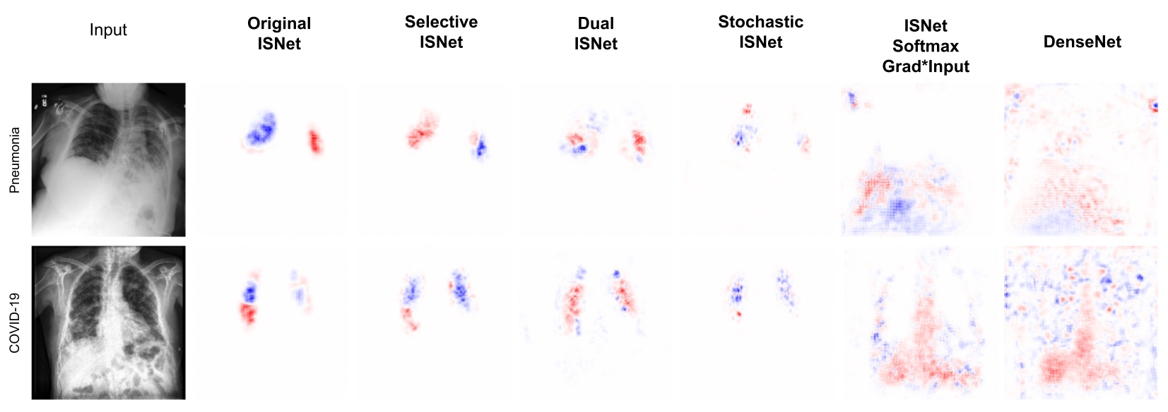
Figure 5: LRP heatmaps for COVID-19 classification. Red colors indicate areas that the DNN associated to the image class (left). Blue areas reduced the confidence for the class, possibly being associated to the other categories. White regions were not important for the classifiers’ decisions.

4 Conclusion

In MNIST classification, the Faster ISNet minimized the influence of background bias on the classifier’s decisions, hindering shortcut learning. Thus, the Faster ISNet’s performance scores did not fall when the synthetic bias was removed from the testing data, or substituted by confounding bias. Accordingly, the model’s LRP heatmaps did not show attention to the synthetic bias. In summary, both the Faster ISNet and the original ISNet presented high accuracy and resistance to shortcut learning in MNIST classification.

COVID-19 detection with chest X-rays is an application where dataset mixing is common[41]. However, in mixed datasets, different classes come from diverse sources, which present distinct background characteristics. Thus, mixing can lead to background bias[4], which causes shortcut learning. The problem reduces the neural networks’ generalization capacity, limiting their performance in out-of-distribution (o.o.d.) datasets (e.g., X-rays from other hospitals), thus reducing real-world accuracy. Accordingly, shortcut learning is a known problem in COVID-19 detection with chest X-rays[3]^,[2]^,[4]^,[46]^,[7]^,[5]. By reducing shortcut learning, the Faster ISNet improved classifier performance in o.o.d. evaluation. In this study we employed COVID-19 detection as a demonstrative application, to showcase the Faster ISNet capacity of minimizing background influence in a contemporary task, employing deep classifiers and high-resolution data. We utilized large, open and high-quality COVID-19 datasets, designed to simulate clinical settings. However, the datasets contain COVID-19 X-rays from the first semester of 2020. Due to more recent variants of the virus and vaccination, disease symptoms may change, altering the DNNs’ classification performance. In summary, the COVID-19 task is this study must be seen as a demonstration of the Faster ISNet capabilities and advantages over the state-of-the-art, not as an indication of clinical performance.

In both biased MNIST and COVID-19 detection, all Faster ISNet variations (Selective, Dual, and Stochastic) outperformed a standard classifier by a large margin (Tables 1 and 2). In COVID-19 detection, the Faster ISNet was compared to multiple state-of-the-art neural networks designed to control classifier attention (U-Net+DenseNet121, Multi-task U-Net, AG-Sononet, Extended GAIN, RRR, and Vision Transformer). The LRP-based ISNets significantly surpassed all the alternative models in o.o.d. evaluation (Table 2), showcasing the novel architecture’s superior capacity of minimizing background attention while maintaining high accuracy.

In accordance with the quantitative o.o.d. test performances, the Faster and original ISNets’ LRP heatmaps did not indicate background attention in COVID-19 detection, while all alternative models’ heatmaps revealed clear background relevance, except for the segmentation-classification pipeline (U-Net+DenseNet121). However, at run-time, the ISNets are much faster (70 to 108%) and lighter (about 5 times less parameters) than the alternative pipeline. Moreover, the Faster and original ISNets significantly surpassed the segmentation-classification pipeline’s accuracy in COVID-19 detection, possibly due to a pipeline’s tendency of focusing on lung borders[4].

The Faster ISNet optimizes LRP heatmaps, a technique based on a series of local Taylor expansions over the DNN neurons[10]. The mathematical fundamentals of LRP allow the ISNet optimization procedure to produce superior resistance to the influence of background bias, while keeping high accuracy[4]. Meanwhile, as input gradients and Gradient*Input explanations become noisy with large neural networks, RRR, and the ISNet Softmax Grad*Input could not match the LRP-based ISNets accuracy when considering very deep classifier backbones (DenseNet121). Furthermore, the optimization of Grad-CAM (GAIN neural network) could not match the LRP-based ISNets, due to the phenomenon of spurious mapping[4]. The advantages of LRP optimization over the optimization of Grad-CAM, input gradients and Gradient*Input are empirically demonstrated by the COVID-19 detection task in this study, and by experiments in the original ISNet study[4]. Such empirical results were theoretically justified in the previous ISNet study[4].

In conclusion, the study presenting the ISNet[4] introduced the concept of optimizing LRP to improve classifier behavior. It empirically demonstrated and theoretically justified the original ISNet’s advantage over multiple state-of-the-art models and implemented ISNets based on the DenseNet and VGG classifier architectures. The current study introduced the ISNet with the popular ResNet backbone, presented LRP Flex, a fast, simple, and model agnostic LRP implementation, and created heuristics that simplify and accelerate the ISNet’s hyper-parameter selection procedure. Finally, we proposed 3 new variants of the original ISNet, the Selective, Dual and Stochastic ISNets, collectively called Faster ISNet. They performed similarly in terms of accuracy and resistance to background bias. The novel models’ accuracy was also similar to the original ISNet’s, lagging slightly behind it in COVID-19 detection. However, the original ISNet training time linearly increases with the number of categories in the classification problem. The Faster ISNet solves this problem, and its training time is independent of the number of classes. Therefore, although slower than the Faster ISNet, the original ISNet can be efficiently trained for classification problems with a small number of categories. However, for applications with more classes, the Faster ISNet’s reduction in training time can be massive, and training the original model can become impracticable (Section 3.4). Thus, the Faster ISNet represents a large reduction in the computational cost of LRP optimization and permits the practical implementation of the technique for a new gamut of classification tasks, where training the original ISNet is not viable.

Appendix A LRP Flex

The original ISNet study reformulated the LRP-$\varepsilon$ relevance propagation procedure (Supplementary Note 8.2 of[4]) to make the denoising property of $\varepsilon$ more explicit, thus justifying the empirically observed advantage of LRP-$\varepsilon$ optimization over the optimization of LRP-0 (Gradient*Input). First, it defined the tensor $\mathbf{G^{L}}$ (with elements $G^{L}_{j}$) as the LRP-$\varepsilon$ relevance at the input of the DNN layer L ($\mathbf{R^{L}}$, with elements $R^{L}_{j}$), divided (element-wise) by the layer’s input ($\mathbf{a^{L}}$, with elements $a^{L}_{j}$). This relationship is shown in Equation 20, considering all layers in the DNN (from 0, the first layer, to Lmax, the output layer). Accordingly, the LRP-$\varepsilon$ heatmap ($\mathbf{R^{0}}$, the LRP relevance at the network’s input) is given by the element-wise multiplication ($\odot$) between $\mathbf{G^{0}}$ and the DNN input, $\mathbf{a^{0}}$ (Equation 21).

$$G^{L}_{j}=R^{L}_{j}/a^{L}_{j}\mbox{ $\forall$ }L\in[0,1,...,\textrm{Lmax}]$$ (20)

$$\mathbf{R^{0}}=\mathbf{G^{0}}\odot\mathbf{a^{0}}$$ (21)

For a neural network utilizing only ReLU nonlinearities, we can find a simple recursive equation to backpropagate $\mathbf{G^{L}}$[4]. First, we add layer superscripts to the standard LRP-$\varepsilon$ rule (Equation 22). Then, we rearrange it considering Equation 20, as shown in Equation 23. Here, $w_{jk}^{L}$ represents the layer L weight connecting its j-th input to its k-th output; $w_{0k}^{L}$ indicates the k-th bias parameters of layer L (considering $a_{0}^{L}=1$); $z_{k}^{L}$ is the k-th output of layer L, before its ReLU activation; and $a^{L+1}_{k}$ is the k-th input of layer L+1, which matches $\mathrm{ReLU}(z_{k}^{L})$.

$$R_{j}^{L}=\sum_{k}\frac{w_{jk}^{L}a_{j}^{L}}{z_{k}^{L}+\textrm{sign}(z_{k}^{L})\epsilon}R_{k}^{L+1}$$ (22)

$$G_{j}^{L}=R^{L}_{j}/a^{L}_{j}=\sum_{k}\frac{w_{jk}^{L}R_{k}^{L+1}}{z_{k}^{L}+\mathrm{sign}(z_{k}^{L})\varepsilon}=\sum_{k}\frac{w_{jk}^{L}a_{k}^{L+1}G_{k}^{L+1}}{z_{k}^{L}+\mathrm{sign}(z_{k}^{L})\varepsilon}=\sum_{k}w_{jk}^{L}\frac{\mathrm{ReLU}(z_{k}^{L})}{z_{k}^{L}+\mathrm{sign}(z_{k}^{L})\varepsilon}G_{k}^{L+1}$$ (23)

Equation 25 defines the Attenuated Step function ($A(\cdot)$)[4]. Accordingly, we reduce Equation 23 into Equation 24, a simple rule to backpropagate $\mathbf{G^{L}}$ through the DNN layers. We can recursively apply Equation 24 until the network’s input layer, producing $\mathbf{G^{0}}$. Afterward, considering Equation 21, an element-wise multiplication of $\mathbf{G^{0}}$ and the DNN input ($\mathbf{a^{0}}$) generates the LRP-$\varepsilon$ heatmap. When explaining a DNN’s logit ($y_{c}$), the chosen logit’s relevance is set to the logit value itself ($y_{c}$), while the other logits’ relevances are set to zero[9]. As we are explaining a logit, the last layer is seen as linear during the relevance propagation, and LRP-0 is a standard choice for such layers[10]. Thus, the LRP relevance at the layer’s inputs ($a^{\textrm{Lmax}}_{j}$) becomes $R^{\textrm{Lmax}}_{j}=w_{jc}^{\textrm{Lmax}}a_{j}^{\textrm{Lmax}}$. Accordingly and following Equation 20, $\mathbf{G^{\textrm{Lmax}}}$ at the input of the DNN last layer matches the layers’ weights (Equation 26).

$$G_{j}^{L}=\sum_{k}w_{jk}^{L}A(z_{k}^{L})G_{k}^{L+1}$$ (24)

$$\mbox{where: }A(z_{k}^{L})=\frac{\mathrm{ReLU}(z_{k}^{L})}{z_{k}^{L}+\mathrm{sign}(z_{k}^{L})\varepsilon}=\begin{cases}\frac{z_{k}^{L}}{z_{k}^{L}+\varepsilon},\mbox{ if }z_{k}^{L}\geq 0\\ 0,\mbox{ otherwise }\end{cases}$$ (25)

$$G_{j}^{\textrm{Lmax}}=w_{jc}^{\textrm{Lmax}}$$ (26)

Equation 24 is similar to the gradient backpropagation rule for fully-connected layers with ReLU activations, shown in Equation 27 (where $y_{c}$ indicates a logit whose gradient is being back-propagated). Indeed, the only difference between the two recursive equations is the substitution of the Attenuated Step function in Equation 24 by the Unit Step function ($H(\cdot)$, defined in Equation 28). Indeed, when $\varepsilon=0$, the Attenuated Step function matches the Unit Step, and the two equations become equivalent. Moreover, the initial values for the gradient and for G match (Equations 26 and 29). Therefore, if $\varepsilon=0$, the quantity G is the gradient ($G_{j}^{L}=\frac{\partial y_{c}}{\partial a_{j}^{L}}\mbox{ $\forall$ }L\in[0,1,...,\textrm{Lmax}]$). Accordingly, it is known that LRP-0 heatmaps match the element-wise multiplication between the DNN input ($\mathbf{a^{0}}$) and the input gradient ($\nabla_{\mathbf{a^{0}}}y_{c}$)[10]. But this equivalence does not hold if $\varepsilon\neq 0$ (LRP-$\varepsilon$ instead of LRP-0)[4].

$$\frac{\partial y_{c}}{\partial a_{j}^{L}}=\sum_{k}w_{jk}^{L}H(z_{k}^{L})\frac{\partial y_{c}}{\partial a_{k}^{L+1}}$$ (27)

$$\mbox{where: }H(z_{k}^{L})=\begin{cases}1,\mbox{ if }z_{k}^{L}>0\\ 0,\mbox{ if }z_{k}^{L}<0\end{cases}$$ (28)

$$\frac{\partial y_{c}}{\partial a_{j}^{\textrm{Lmax}}}=w_{jc}^{\textrm{Lmax}}$$ (29)

The original ISNet paper proposed the alternative LRP-$\varepsilon$ formulation (Equations 24 and 21) to justify the empirically observed advantage of LRP-$\varepsilon$ (ISNet) optimization over optimizing LRP-0 or Gradient*Input (ISNet Grad*Input). LRP-0 and Gradient*Input are noisy for deep neural networks, and LRP-$\varepsilon$ produces less noisy explanations, which are easier to optimize. Accordingly, the ISNet displayed a more stable and easier loss convergence with respect to the ISNet Grad*Input, especially with very deep classifiers. Thus, the ISNet surpassed the ISNet Grad*Input in terms of accuracy and resistance to background bias[4]. The Attenuated Step (Equation 25) is a monotonically increasing function, which approximates the Unit Step for negative or high arguments. However, unlike the Unit Step, it reduces the influence of small neuron activations ($\mathrm{ReLU}(z_{k}^{L})$) on the back-propagated quantity ($G_{j}^{L}$) and on the final heatmap. The higher the $\varepsilon$, the stronger the attenuation[4]. Therefore, $\varepsilon$ controls a denoising process, justified by the Deep Taylor Decomposition framework (where LRP-$\varepsilon$ represents a reduction in the first-order Taylor approximation error in relation to LRP-0 and Gradient*Input), attenuating explanation noise and improving coherence and contextualization[4]^,[10].

In this study, we show that the alternative LRP formulation (Equations 24 and 21), conceived as a theoretical justification in the original ISNet paper[4], can derive an alternative LRP implementation, LRP Flex. The implementation is exceedingly simple and model agnostic, being readily applicable to any deep neural network with only ReLU activations (except for the last layer).

First, the gradient backpropagation rule in Equation 27 can be separated in two parts: a gradient back-propagation through the ReLU activation (Equation 30), followed by the back-propagation of $\frac{\partial y_{c}}{\partial z_{k}^{L}}$ through the fully-connected layer L (Equation 31).

$$\frac{\partial y_{c}}{\partial z_{k}^{L}}=H(z_{k}^{L})\frac{\partial y_{c}}{\partial a_{k}^{L+1}}$$ (30)

$$\frac{\partial y_{c}}{\partial a_{j}^{L}}=\sum_{k}w_{jk}^{L}\frac{\partial y_{c}}{\partial z_{k}^{L}}$$ (31)

We can also separate the alternative LRP-$\varepsilon$ G backpropagation rule (Equation 24) in two sequential steps, represented in Equations 32 and 33. They represent a sequential backpropagation of G through the ReLU function and the preceding fully-connected layer, respectively.

$$U_{k}^{L}=A(z_{k}^{L})G_{k}^{L+1}$$ (32)

$$G_{j}^{L}=\sum_{k}w_{jk}^{L}U_{k}^{L}$$ (33)

Equations 33 and 31 show that the backpropagation step through the fully-connected layer is the same for both the gradient and G. Meanwhile, the backpropagation step through the ReLU activation is not. Equation 32 represents a modification in the standard backward pass through ReLU functions (Equation 30): instead of multiplying the back-propagated quantity ($G_{k}^{L+1}$) by the Unit Step $H(z_{k}^{L})$, we multiply it (element-wise) by the Attenuated Step $A(z_{k}^{L})$. Therefore, with a simple modification of the ReLU’s backward step (substituting $H(\cdot)$ by $A(\cdot)$), automatic gradient backpropagation engines can backpropagate G instead of the actual gradient. Notice that the Attenuated Step can be directly calculated from the output of the ReLU (Equation 34). In summary, we can easily leverage the automatic differentiation capabilities offered by deep learning libraries to produce LRP heatmaps. Gradient backpropagation algorithms tend to be fast, highly optimized, and readily applicable to new DNN architectures. To obtain G at the DNN input ($\mathbf{G^{0}}$), we modify the ReLU back-propagation rule, and request the backpropagation engine to compute the gradient of the DNN’s explained logit ($y_{c}$) with respect to the network’s input ($\mathbf{a^{0}}$). Then, the LRP-$\varepsilon$ heatmap is obtained by the element-wise multiplication between $\mathbf{G^{0}}$ and the DNN input (Equation 21).

$$A(z_{k}^{L})=A(ReLU(z_{k}^{L}))=\frac{\mathrm{ReLU}(z_{k}^{L})}{\mathrm{ReLU}(z_{k}^{L})+\varepsilon}$$ (34)

In PyTorch, a backward hook (applied with register_full_backward_hook) can modify the ReLU module’s backward pass, implementing Equation 32 and making the automatic differentiation procedure backpropagate G instead of the gradient. To calculate the Attenuated Step function, we can use the output of the ReLU ($ReLU(z_{k}^{L})$) as argument (Equation 34). This output can be stored by a forward hook (applied with register_forward_hook) during the forward pass. The backward hooks activate automatically in backward passes, but they can be deactivated (e.g., by changing a global flag variable) during a standard loss backpropagation in the training procedure. With a recursive function, we can easily apply the hooks to all ReLU layers in an instantiated network. We must only avoid in-place operations inside the DNN from changing the ReLU outputs stored during the forward pass. Finally, the backpropagation algorithm in PyTorch is differentiable. Therefore, LRP Flex can be used to quickly and easily explain a trained DNN’s decisions, and to produce the LRP heatmaps used for training the original, Selective and Stochastic ISNets.

Equation 26 is valid for creating a heatmap that explains a DNN’s logit, such as the explanations in the original and Stochastic ISNets. However, the Selective ISNet maps explain a softmax-based quantity ($\eta_{c}$, Equation 9 ) instead of a logit ($y_{c}$). Equation 12 explains the calculation of the relevance at the input of the DNN’s last layer ($R_{j}$, which becomes $R^{\textrm{Lmax}}_{j}$ with the inclusion of the layer superscript) when explaining $\eta_{c}$. In this case, the quantity $G^{\textrm{Lmax}}_{j}$, defined as $R^{\textrm{Lmax}}_{j}/a^{\textrm{Lmax}}_{j}$ (Equation 20), is equivalent to the gradient of $\eta_{c}$ with respect to the inputs of the last DNN layer (Equation 35).

$$G^{\textrm{Lmax}}_{j}=\frac{\partial\eta_{c}}{\partial a_{j}^{\textrm{Lmax}}}$$ (35)

To prove this equality, we first take the derivative of $\eta_{c}$ with respect to $z_{c,c^{\prime}}$ (defined in Equation 11, which here we write with the following notation: $z_{c,c^{\prime}}=y_{c}-y_{c^{\prime}}$), as shown in Equation 36. Afterward, we can take derivative of $\eta_{c}$ with respect to the inputs of the last DNN layer ($a_{j}^{\textrm{Lmax}}$), using the calculus chain rule, as displayed in Equation 37.

$$\frac{\partial\eta_{c}}{\partial z_{c,c^{\prime}}}=\frac{\partial[-\ln(\sum_{c^{\prime\prime}\neq c}e^{-z_{c,c^{\prime\prime}}})]}{\partial z_{c,c^{\prime}}}=\frac{e^{-z_{c,c^{\prime}}}}{\sum_{c^{\prime\prime}\neq c}e^{-z_{c,c^{\prime\prime}}}}$$ (36)

$$\frac{\partial\eta_{c}}{\partial a_{j}^{\textrm{Lmax}}}=\sum_{c^{\prime}}\frac{\partial\eta_{c}}{\partial z_{c,c^{\prime}}}\frac{\partial z_{c,c^{\prime}}}{\partial a_{j}^{\textrm{Lmax}}}=\sum_{c^{\prime}}\frac{\partial\eta_{c}}{\partial z_{c,c^{\prime}}}(w_{jc}^{\textrm{Lmax}}-w_{jc^{\prime}}^{\textrm{Lmax}})=\sum_{c^{\prime}}\frac{e^{-z_{c,c^{\prime}}}}{\sum_{c^{\prime\prime}\neq c}e^{-z_{c,c^{\prime\prime}}}}(w_{jc}^{\textrm{Lmax}}-w_{jc^{\prime}}^{\textrm{Lmax}})$$ (37)

Now, we combine Equations 12 and 13 into Equation 38. Equations 12 and 13 are the standard rules to propagate LRP relevance until $a_{j}^{\textrm{Lmax}}$ when explaining $\eta_{c}$[10]. Here, we set the stabilizers $\mu$ and $\epsilon$ to zero in Equations 12 and 13. Notice that $\mu$ is not part of the standard propagation rule[10] (it was added to improve numerical stability in this work), and setting $\epsilon=0$ would represent the use of LRP-0 in the last DNN layer, a standard choice[10].

$$R_{j}^{\textrm{Lmax}}=\sum_{c^{\prime}}\frac{(w_{jc}^{\textrm{Lmax}}-w_{jc^{\prime}}^{\textrm{Lmax}})a_{j}^{\textrm{Lmax}}}{z_{c,c^{\prime}}+\textrm{sign}(z_{c,c^{\prime}})\epsilon}\frac{z_{c,c^{\prime}}e^{-z_{c,c^{\prime}}}}{\sum_{c^{\prime\prime}\neq c}e^{-z_{c,c^{\prime\prime}}}+\mu}=a_{j}^{\textrm{Lmax}}\sum_{c^{\prime}}\frac{e^{-z_{c,c^{\prime}}}}{\sum_{c^{\prime\prime}\neq c}e^{-z_{c,c^{\prime\prime}}}}(w_{jc}^{\textrm{Lmax}}-w_{jc^{\prime}}^{\textrm{Lmax}})$$ (38)

To derive $G_{j}^{\textrm{Lmax}}$ from Equation 38 (which represents standard LRP relevance propagation rules[10]), we divide both of its sides by $a_{j}^{\textrm{Lmax}}$ in Equation 39 (considering the definition $R_{j}^{L}=a_{j}^{L}G_{j}^{L}$ in Equation 20). Finally, comparing Equations 37 and 39, we prove the equality $G^{\textrm{Lmax}}_{j}=\frac{\partial\eta_{c}}{\partial a_{j}^{\textrm{Lmax}}}$ shown in Equation 35.

$$G^{\textrm{Lmax}}_{j}=R_{j}^{\textrm{Lmax}}/a_{j}^{\textrm{Lmax}}=\sum_{c^{\prime}}\frac{e^{-z_{c,c^{\prime}}}}{\sum_{c^{\prime\prime}\neq c}e^{-z_{c,c^{\prime\prime}}}}(w_{jc}^{\textrm{Lmax}}-w_{jc^{\prime}}^{\textrm{Lmax}})=\frac{\partial\eta_{c}}{\partial a_{j}^{\textrm{Lmax}}}$$ (39)

Exploiting Equation 35, to explain $\eta_{c}$ instead of $y_{c}$, LRP Flex simply requests the backpropagation engine for the gradient of $\eta_{c}$ with respect to the DNN input, applying the modified ReLU backpropagation rule in Equation 32. Then, the resulting tensor ($\mathbf{G^{0}}$) is element-wise multiplied with the DNN’s input, producing the LRP-$\varepsilon$ heatmap (Equation 21). However, $\eta_{c}$ backpropagation can be numerically unstable, as $\eta_{c}$ explodes when the softmax probability of class c approaches 0 or 1 (Equation 9). Therefore, to ensure numerical stability, we can backpropagate a bounded version of $\eta_{c}$, defined in Equation 40. In the equation, $P_{c}$ is the probability of class c (i.e., the Softmax output for logit $y_{c}$, Equation 8), and $\mu$ is a positive constant. The higher the $\mu$ hyper-parameter, the smaller the maximum magnitude of $\tilde{\eta_{c}}$ and its gradient.

$$\tilde{\eta_{c}}=ln(P_{c}+\mu)-\ln(1-P_{c}+\mu)$$ (40)

For simplicity, the equations in this section considered fully-connected layers. However, convolutions can be represented as fully connected layers. Moreover, other common layers, such as batch normalization, dropout and pooling can also be expressed as fully connected layers, or fused with adjacent fully-connected layers or convolutions. Thus, the reasoning in this section and the LRP Flex implementation are not restricted to fully-connected DNNs. Indeed, LRP Flex just requires the DNN’s hidden layers to contain only ReLU nonlinearities. However, LRP-$\varepsilon$ was designed for DNNs with ReLU activations anyway[9], and such architectures compose a large proportion of the state-of-the-art (e.g., ResNets and DenseNets).

References

- [1] R. Geirhos, J.-H. Jacobsen, C. Michaelis, R. Zemel, W. Brendel, M. Bethge, and F. Wichmann, “Shortcut learning in deep neural networks,” Nature Machine Intelligence, vol. 2, pp. 665–673, 11 2020.
- [2] J. López-Cabrera, J. Portal Diaz, R. Orozco, O. Lovelle, and M. Perez-Diaz, “Current limitations to identify covid-19 using artificial intelligence with chest x-ray imaging (part ii). the shortcut learning problem,” Health and Technology, vol. 11, 10 2021.
- [3] A. J. DeGrave, J. D. Janizek, and S.-I. Lee, “Ai for radiographic covid-19 detection selects shortcuts over signal,” Nat Mach Intell, vol. 3, p. 610–619, 05/2021 2021.
- [4] P. R. A. S. Bassi, S. S. J. Dertkigil, and A. Cavalli, “Improving deep neural network generalization and robustness to background bias via layer-wise relevance propagation optimization,” Nature Communications, vol. 15, Jan. 2024.
- [5] P. R. A. S. Bassi and R. Attux, “Covid-19 detection using chest x-rays: is lung segmentation important for generalization?,” 2021.
- [6] A. Signoroni, M. Savardi, S. Benini, N. Adami, R. Leonardi, P. Gibellini, F. Vaccher, M. Ravanelli, A. Borghesi, R. Maroldi, and D. Farina, “Bs-net: learning covid-19 pneumonia severity on a large chest x-ray dataset,” Medical Image Analysis, vol. 71, p. 102046, 03 2021.
- [7] G. Maguolo and L. Nanni, “A critic evaluation of methods for covid-19 automatic detection from x-ray images,” 2020.
- [8] W. H. Organization, Chest radiography in tuberculosis detection: summary of current WHO recommendations and guidance on programmatic approaches. World Health Organization, 2016.
- [9] S. Bach, A. Binder, G. Montavon, F. Klauschen, K.-R. Müller, and W. Samek, “On pixel-wise explanations for non-linear classifier decisions by layer-wise relevance propagation,” PLOS ONE, vol. 10, pp. 1–46, 07 2015.
- [10] G. Montavon, A. Binder, S. Lapuschkin, W. Samek, and K.-R. Müller, “Layer-wise relevance propagation: An overview,” in Explainable AI: Interpreting, Explaining and Visualizing Deep Learning, pp. 193–209, Springer International Publishing, 2019.
- [11] K. Simonyan, A. Vedaldi, and A. Zisserman, “Deep inside convolutional networks: Visualising image classification models and saliency maps,” 2014.
- [12] A. S. Ross, M. C. Hughes, and F. Doshi-Velez, “Right for the right reasons: Training differentiable models by constraining their explanations,” in Proceedings of the Twenty-Sixth International Joint Conference on Artificial Intelligence, IJCAI-17, pp. 2662–2670, 2017.
- [13] A. Shrikumar, P. Greenside, A. Shcherbina, and A. Kundaje, “Not just a black box: Learning important features through propagating activation differences,” ArXiv, vol. abs/1605.01713, 2016.
- [14] R. R. Selvaraju, M. Cogswell, A. Das, R. Vedantam, D. Parikh, and D. Batra, “Grad-cam: Visual explanations from deep networks via gradient-based localization,” in 2017 IEEE International Conference on Computer Vision (ICCV), pp. 618–626, 2017.
- [15] K. Li, Z. Wu, K.-C. Peng, J. Ernst, and Y. Fu, “Tell me where to look: Guided attention inference network,” 03 2018.
- [16] X. Ouyang, S. Karanam, Z. Wu, T. Chen, J. Huo, X. S. Zhou, Q. Wang, and J.-Z. Cheng, “Learning hierarchical attention for weakly-supervised chest x-ray abnormality localization and diagnosis,” IEEE Transactions on Medical Imaging, vol. 40, no. 10, pp. 2698–2710, 2021.
- [17] A. Dosovitskiy, L. Beyer, A. Kolesnikov, D. Weissenborn, X. Zhai, T. Unterthiner, M. Dehghani, M. Minderer, G. Heigold, S. Gelly, J. Uszkoreit, and N. Houlsby, “An image is worth 16x16 words: Transformers for image recognition at scale,” 2020.
- [18] J. Schlemper, O. Oktay, M. Schaap, M. Heinrich, B. Kainz, B. Glocker, and D. Rueckert, “Attention gated networks: Learning to leverage salient regions in medical images,” 2018.
- [19] G. Huang, Z. Liu, L. Van Der Maaten, and K. Q. Weinberger, “Densely connected convolutional networks,” in 2017 IEEE Conference on Computer Vision and Pattern Recognition (CVPR), pp. 2261–2269, 2017.
- [20] K. Simonyan and A. Zisserman, “Very deep convolutional networks for large-scale image recognition,” arXiv 1409.1556, 09 2014.
- [21] K. He, X. Zhang, S. Ren, and J. Sun, “Deep residual learning for image recognition,” pp. 770–778, 06 2016.
- [22] L. Deng, “The mnist database of handwritten digit images for machine learning research,” IEEE Signal Processing Magazine, vol. 29, no. 6, pp. 141–142, 2012.
- [23] J. P. Cohen, M. Hashir, R. Brooks, and H. Bertrand, “On the limits of cross-domain generalization in automated x-ray prediction,” in Proceedings of the Third Conference on Medical Imaging with Deep Learning (T. Arbel, I. Ben Ayed, M. de Bruijne, M. Descoteaux, H. Lombaert, and C. Pal, eds.), vol. 121 of Proceedings of Machine Learning Research, pp. 136–155, PMLR, 06–08 Jul 2020.
- [24] P. Rajpurkar, J. Irvin, K. Zhu, B. Yang, H. Mehta, T. Duan, D. Y. Ding, A. Bagul, C. Langlotz, K. S. Shpanskaya, M. P. Lungren, and A. Y. Ng, “Chexnet: Radiologist-level pneumonia detection on chest x-rays with deep learning,” CoRR, vol. abs/1711.05225, 2017.
- [25] G. Montavon, S. Lapuschkin, A. Binder, W. Samek, and K.-R. Müller, “Explaining nonlinear classification decisions with deep taylor decomposition,” Pattern Recognition, vol. 65, p. 211–222, 05 2017.
- [26] S. Zagoruyko and N. Komodakis, “Paying more attention to attention: Improving the performance of convolutional neural networks via attention transfer,” 2017.
- [27] M. Ancona, E. Ceolini, C. Öztireli, and M. Gross, “Towards better understanding of gradient-based attribution methods for deep neural networks,” 2018.
- [28] S. Qiu, “Global weighted average pooling bridges pixel-level localization and image-level classification,” 2018.
- [29] B. P. Welford, “Note on a method for calculating corrected sums of squares and products,” Technometrics, vol. 4, no. 3, pp. 419–420, 1962.
- [30] K. Simonyan and A. Zisserman, “Very deep convolutional networks for large-scale image recognition,” 2014.
- [31] R. Caruana, “Multitask learning,” Machine Learning, vol. 28, 07 1997.
- [32] O. Ronneberger, P.Fischer, and T. Brox, “U-net: Convolutional networks for biomedical image segmentation,” in Medical Image Computing and Computer-Assisted Intervention (MICCAI), vol. 9351 of LNCS, pp. 234–241, Springer, 2015.
- [33] M.-H. Guo, T.-X. Xu, J.-J. Liu, Z.-N. Liu, P.-T. Jiang, T.-J. Mu, S.-H. Zhang, R. Martin, M.-M. Cheng, and S.-M. Hu, “Attention mechanisms in computer vision: A survey,” Computational Visual Media, 03 2022.
- [34] Z. Kong, M. He, Q. Luo, X. Huang, P. Wei, Y. Cheng, L. Chen, Y. Liang, Y. Lu, X. Li, and J. Chen, “Multi-task classification and segmentation for explicable capsule endoscopy diagnostics,” Frontiers in Molecular Biosciences, vol. 8, 2021.
- [35] Y. Zhou, H. Chen, Y. Li, Q. Liu, X. Xu, S. Wang, and P.-T. Yap, “Multi-task learning for segmentation and classification of tumors in 3d automated breast ultrasound images,” Medical Image Analysis, vol. 70, p. 101918, 11 2020.
- [36] D. Zhang, J. Wang, and X. Zhao, “Estimating the uncertainty of average f1 scores,” Proceedings of the 2015 International Conference on The Theory of Information Retrieval, 2015.
- [37] J. Salvatier, T. Wiecki, and C. Fonnesbeck, “Probabilistic programming in python using pymc3,” PeerJ Computer Science, 2016.
- [38] M. D. Homan and A. Gelman, “The no-u-turn sampler: Adaptively setting path lengths in hamiltonian monte carlo,” J. Mach. Learn. Res., vol. 15, p. 1593–1623, Jan. 2014.
- [39] D. J. Hand and R. J. Till, “A simple generalisation of the area under the roc curve for multiple class classification problems,” Mach. Learn., vol. 45, p. 171–186, Oct. 2001.
- [40] P. R. A. S. Bassi and R. Attux, “A deep convolutional neural network for covid-19 detection using chest x-rays,” Research on Biomedical Engineering, Apr 2021.
- [41] A. Shoeibi, M. Khodatars, R. Alizadehsani, N. Ghassemi, M. Jafari, P. Moridian, A. Khadem, D. Sadeghi, S. Hussain, A. Zare, Z. A. Sani, J. Bazeli, F. Khozeimeh, A. Khosravi, S. Nahavandi, U. R. Acharya, and P. Shi, “Automated detection and forecasting of covid-19 using deep learning techniques: A review,” 2020.
- [42] J. Irvin, P. Rajpurkar, M. Ko, Y. Yu, S. Ciurea-Ilcus, C. Chute, H. Marklund, B. Haghgoo, R. Ball, K. Shpanskaya, J. Seekins, D. Mong, S. Halabi, J. Sandberg, R. Jones, D. Larson, C. Langlotz, B. Patel, M. Lungren, and A. Ng, “Chexpert: A large chest radiograph dataset with uncertainty labels and expert comparison,” Proceedings of the AAAI Conference on Artificial Intelligence, vol. 33, pp. 590–597, 07 2019.
- [43] M. de la Iglesia Vayá, J. M. Saborit, J. A. Montell, A. Pertusa, A. Bustos, M. Cazorla, J. Galant, X. Barber, D. Orozco-Beltrán, F. García-García, M. Caparrós, G. González, and J. M. Salinas, “Bimcv covid-19+: a large annotated dataset of rx and ct images from covid-19 patients,” 2020.
- [44] X. Wang, Y. Peng, L. Lu, Z. Lu, M. Bagheri, and R. M. Summers, “Chestx-ray8: Hospital-scale chest x-ray database and benchmarks on weakly-supervised classification and localization of common thorax diseases,” 2017 IEEE Conference on Computer Vision and Pattern Recognition (CVPR), Jul 2017.
- [45] S. Jaeger, S. Candemir, S. Antani, Y.-X. J. Wáng, P.-X. Lu, and G. R. Thoma, “Two public chest x-ray datasets for computer-aided screening of pulmonary diseases.,” Quantitative imaging in medicine and surgery, vol. 4 6, pp. 475–7, 2014.
- [46] L. O. Teixeira, R. M. Pereira, D. Bertolini, L. S. Oliveira, L. Nanni, G. D. C. Cavalcanti, and Y. M. G. Costa, “Impact of lung segmentation on the diagnosis and explanation of covid-19 in chest x-ray images,” Sensors, vol. 21, no. 21, 2021.