Graph Structure of an Inversive Pseudorandom Number Generator over Ring
Abstract
Generating random and pseudorandom numbers with a deterministic system is a long-standing challenge in theoretical research and engineering applications. Several pseudorandom number generators based on the inversive congruential method have been designed as attractive alternatives to those based on the classical linear congruential method. This paper discloses the least period of sequences generated by iterating an inversive pseudorandom number generator over the ring by transforming it into a two-order linear congruential recurrence relation. Depending on whether the sequence is periodic or ultimately periodic, all states in the domain can be attributed to two types of objects: some cycles of different lengths and one unilateral connected digraph whose structure remains unchanged concerning parameter . The graph structure of the generator over the ring is precisely disclosed with rigorous theoretical analysis and verified experimentally. The adopted analysis methodology can be extended to study the graph structure of other nonlinear maps.
Index Terms:
Galois ring, Inversive congruential method, Linear congruential, Functional graph, Pseudorandom number generator, Period.I Introduction
Pseudorandom number generators () are deterministic algorithms designed to produce long sequences of numbers that exhibit the characteristics of randomness and are indistinguishable from true random numbers in a stream [1, 2, 3, 4, 5]. These generators find wide applications in scientific and engineering domains, including Monte Carlo simulations, computer games, and cryptography [6]. The linear congruential method, a prominent technique for generating random numbers, can be traced back to Lehmer’s proposed in 1951 [7]. This method operates in a multiplicative group of integers modulo , with the recurrence relation , where is a large integer, and are chosen from the set , and is a non-negative integer. Subsequently, Park and Miller introduced Lehmer’s with specific parameters and , known as the minimal standard generator (MINSTD), widely used as the default in the C++ programming language [8]. Additionally, several of the Lehmer form are integrated into the GNU Scientific Library, a numerical computing library for C and C++ programmers [9]. In 1965, Tausworthe presented a that combines -bit continuous binary sequences generated by the linear shift register method over a binary field [10]. This , when compared to Lehmer’s, necessitates a sufficiently large to meet the randomness requirements for numbers falling within the interval [0, 1]. Building upon Tausworthe’s work, Knuth developed a generalized class of random number generators using a -th order linear congruential recurrence relation over a larger finite field, extending beyond binary fields:
| (1) |
where is a prime number, and parameters and initial states belong to the set [11]. This generator encompasses Lehmer’s and Tausworthe’s as special cases. Subsequent research has explored statistical characteristics [12, 13], criteria for randomness assessment [14], expansion to other domains [15, 16], and applications in cryptography based on coding theory [17].
The nuanced relationship between chaotic systems and cryptosystems has positioned it as a novel avenue for designing secure and efficient pseudorandom number generators () [18, 19, 20]. Since von Neumann employed the Logistic map for generating random numbers in [21], a variety of based on chaotic maps has been proposed. Examples include the Tent map [22], Logistic map [23, 24], Cat map [25, 26], Chebyshev map [27, 28], and Rényi chaotic map [29]. Notably, the Chebyshev map and Cat map are inherently linear. However, linear generators may lack cryptographic security in certain domains, prompting an intuitive preference for nonlinear alternatives [30, 31, 32, 33].
As a promising nonlinear method for generating pseudorandom numbers, the inversive pseudorandom number generator () over a finite field was initially proposed in [34]:
| (2) |
where is a prime, is the inverse of in , and . Leeb and Wegenkittl, through a series of empirical tests, demonstrated that can pass tests with a broader range of parameters compared to their linear counterparts [35]. The intriguing properties of swiftly captured the attention of researchers, and it found widespread use in applications such as Quasi-Monte Carlo methods and public key encryption [36, 37, 38, 33, 35]. Additionally, Solé et al. extended over the Galois ring , a commutative ring with characteristic and elements. They posed an open problem regarding the conditions on parameters to achieve the maximal period [39]. The generalization and various variants of were comprehensively reviewed in [40].
Complete understanding of the period distribution and related statistical characteristics of is a basis for its extensive applications [41, 42, 43, 44, 45, 39]. In [41] and [46], Chou described all possible periods of an over a finite field by linear difference equation and demonstrated their relation with the period of the corresponding characteristic polynomials. The sufficient and necessary condition of parameters and initial state to achieve the maximal period of an with modulo is given [44]. Then Eichenauer generalized the modulus in [44] to the power of a prime and presented the conditions that the corresponding parameters of certain specific periods meet [45]. However, the complete information on period distribution for any parameter and initial state is not given, which limits the applications of with prime power modulus. Furthermore, it is noteworthy that the sequence generated by iterating may not be purely periodic, which differs from the cases of Chebyshev map and Cat map. Especially, Chen et al. demonstrated that if the maximal period of the sequence generated by the Chebyshev polynomial over finite field is lower than , the underpinned public key encryption algorithm is insecure [27]. Therefore, the period analysis of the sequence generated by for all initial states is critical for any associated application.
The functional graph (also known as state-mapping network) of a map is an essential visible way to study the period distribution of sequences generated by iterating the map. The produced periodic sequence corresponds to a cycle in the corresponding functional graph. In [25], Li et al. disclosed the graph structure of the generalized Cat map in any binary arithmetic domain and proved how the period of the sequence generated by iterating the map changes with the arithmetic precision. Similarly, the graph structures of the Logistic map and Tent map in a digital domain are also studied [23, 47]. In the past five years, the functional graphs of various polynomials over a finite field, Chebyshev polynomials [48], linearized polynomials [49], and a class of polynomials of form [50], are disclosed in terms of the distribution of cycles, where is a polynomial.
Although has been proposed for almost four decades, the structure of its functional graph remains unknown. To make the analysis of the graph structure more general and complete, the domain of is extended from finite field to ring in this paper:
| (3) |
where , is multiplicative group of ring and is the inverse of in . Given an initial state and parameters and , one can get an inversive pseudorandom number sequence () by recursion (3). Then, its period is obtained using the Galois ring theory and characteristic polynomials. The connected component of the functional graph of over is either a unilateral connected digraph with an invariable structure or a cycle with no more than three possible lengths. So, the structure of the functional graph can be unraveled by counting the number of its different connected components.
The rest of the paper is organized as follows. Section II presents some preliminaries and lemmas that help to understand the analysis. Then, Sec. III discloses the graph structure of (3) over . Furthermore, Sec. IV presents a detailed analysis of the graph structure of the generator over Galois ring . The last section concludes the paper.
II Preliminary
This section introduces the relevant notations and definitions to facilitate the discussion in the ensuing sections. As for more knowledge on the finite field and Galois ring, refer to [51] and [52].
II-A Galois ring and irreducible polynomial
In ring theory, a finite ring containing identity is called Galois ring if its zero-divisors and zero elements form a principal ideal. Denote be a Galois ring of characteristic with cardinality , where is a prime number, and are a natural number. One can know that (See [52, Example 14.1]), where is the ring of residue classes of integers modulo concerning modular addition and multiplication. Any element can be uniquely expressed as a -adic representation
| (4) |
where , and if ; otherwise, and is an element of order in . All elements in with and that with form its multiplicative group and a unique maximal ideal , respectively. The least positive integer such that in a group is called the order of the element . Lemma 1 describes the order of some special elements in .
Lemma 1.
For any ,
where and represents the order of element in .
Proof.
Since , one has and , where and . Thus, is equivalent to
Then is the least positive integer satisfying the above congruence, which yields . Similarly, when , and . ∎
Let be a polynomial over , where coefficients , is a non-negative integer, and is an indeterminate. The polynomial composes a polynomial ring concerning multiplication and addition over [51, Definition 1.48]. Let denote the image of under a map from polynomial ring to another polynomial ring :
| (5) |
where hereinafter. For any polynomials , , they are co-prime in if and only if and are co-prime in [52, Lemma 13.5]. Using such co-prime property of any two polynomials in , one can prove Hensel’s Lemma (Lemma 2), which plays a vital role in the period analysis of the linear recursive sequence over ring .
Lemma 2.
(Hensel’s Lemma) Let be a polynomial in and if , where and are co-prime polynomials in . Then there exists co-prime polynomials and in , such that , and .
A polynomial is called irreducible over a field if it cannot be factored. In contrast, if its image under map (5) is irreducible in , the polynomial is called basic irreducible. Using Lemma 2, one can get a necessary and sufficient condition that an irreducible polynomial of degree two in is basic irreducible, as shown in Lemma 3.
Lemma 3.
Irreducible polynomial is basic irreducible in if and only if .
Proof.
When , assume is reducible in , one has , where and . Referring to Hensel’s Lemma, one can know that there exist co-prime polynomials and in , such that in and , which contradicts with that is irreducible. So is a basic irreducible polynomial in . When , one has , which yields is reducible in and is not a basic irreducible polynomial in . ∎
II-B Functional graph of over ring
Let denote a specific generated by iterating (3) from an initial state , where , and . Its least period is the smallest integer such that for any . If , sequence is ultimately periodic, periodic otherwise. To study the period of an over , a second-order linear recurring sequence () generated by
| (6) |
from initial state is defined, where . Then, the relation between the and is revealed in Lemma 4, which serves as the basis of the analysis of this paper.
Lemma 4.
Proof.
This lemma can be proved via mathematical induction , and its proof is omitted. ∎
The characteristic polynomial (or generating polynomial) of an generated by relation (6) is . We call the polynomial the indirect characteristic polynomial of the corresponding hereinafter. Note that is not always irreducible in , but it is always reducible in the extension ring , where is the ideal generated by . Thus, we can write as an uniform reducible form:
| (8) |
where belong to
| (9) |
If is basic irreducible in , ring is isomorphic to the [52, Corollary 14.7]. Specially, is abbreviated as when . It follows from Eq. (8) that
| (10) |
Definition 1.
Let denote the functional graph of (3) over Galois ring .
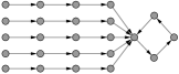
Functional graph given in Definition 1 is constructed as [23]: the elements in ring are considered as separate nodes; node is directly linked to node if and only if . In addition, we introduce a digraph (directed graph) that may be connected component in .
Definition 2.
Let denote a unilateral connected digraph composing a cycle of length whose sole node is linked by transient branches of length as a target.

a)
b)
III Graph structure of (3) over
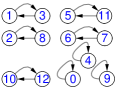
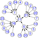
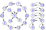
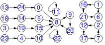
In this section, the structure of is disclosed via the period of every sequence generated by iterating (3). Figure 2 demonstrates that with representative parameters to facilitate the description of theoretical analysis. The analysis process of the period for two cases and is significantly different, so they are separately analyzed in the following two sub-sections.

a)
b)

c)
d)
e)
III-A Graph structure of (3) over with
As there are no zero-divisors in , can be divided into two cases: ; . As for the first case, one has from (3) for any . It means . So, it’s period and every state evolves to state . As for the second case, one can get the concrete numbers of cycles of length two and self-loop composing the whole functional graph of (3), as shown in Proposition 1.
Proposition 1.
When and , is composed of cycles of length two and self-loops, where and denotes the cardinality of a set.
Proof.
III-B Graph structure of (3) over with
From Lemma 4, one can know an generated by iterating (3) can be converted to a generated by iterating relation (6) with . The solution of the corresponding indirect characteristic polynomial has two possible cases: one root with multiplicity two; two distinct roots with multiplicity one. The general term of the associated is different in the two cases, which is determined by whether congruence exists. Thus, the structure of in such two cases are separately discussed in the following.
III-B1
In such case, one can know is reducible in , namely in Eq. (8). Then,
| (11) |
Furthermore, one can get the general term of relation (6) as
where . Substituting and into the above equation yields
| (12) |
As shown in Proposition 2, we can prove that the generator can produce maximum-length sequences (also called m-sequences).
Proposition 2.
When , is composed of one cycle of length and one self-loop.
Proof.
When , one can know from Eq. (11), which means sequence and .
When , there must exist an integer number such that . It yields from Eq. (12) that sequence must contain zero element. So does sequence from Lemma 4-ii), which further deduces . Let , then from Eqs. (11) and (12). It means is the smallest integer such that . From Lemma 4-ii), one can know is the smallest integer satisfying . Then, one can get . For any , there are initial states of value satisfying . All such states make up a cycle of length in with their mapping relation.
Combining the above two cases, one can know is composed of one cycle of length and one self-loop. ∎
III-B2
In such case, one has and from Eq. (8). Then, the general term of relation (6) is , where . Substituting and into the previous equation, one has and . So,
| (13) |
Referring to Lemma 4, one can know that whether for some is the key to calculate the period of sequence . Depending on such condition, Lemma 5 reveals the three possible values of the period of sequence according to the relation between and .
Lemma 5.
When and , sequence is periodic and its least period
where and
Proof.
When , one has in value from Eq. (13). Equation (7) yields for any . Thus, sequence is periodic and .
When , one has is a unit, an invertible element for the multiplication of the associated ring. From Eq. (13), one can obtain that if and only if
Then, the above congruence is equivalent to
| (14) |
Hence, if and only if
| (15) |
According to whether condition (15) exists, the proof is divided into the following two cases:
-
•
: There exists a positive integer such that from condition (15). Then one has from Eq. (7). Thus, sequence contains zero element and . Setting and , one has from Eq. (13). It means is the smallest integer satisfying . Thus, . Since , and is closed concerning the power of its any element, there are initial states of value such that . Thus, sequence is periodic.
- •
∎
In number theory, an integer is called a quadratic residue modulo if it is congruent to a perfect square modulo , that is , where . Then, if is a quadratic residue modulo , polynomial is reducible over and . It follows from Lemma 5 that is composed of two cycles of different lengths and two self-loops, as presented in Proposition 3. If is a non-quadratic residue modulo , is irreducible over and . So, there is no self-loop in .
Proposition 3.
When and , is composed of one cycle of length , cycles of length , and self-loops, where , if is a quadratic residue modulo ; otherwise.
Proof.
If is a quadratic residue modulo , one has . Referring to Lemma 5, one can see there are three possible least periods in . So, there is one self-loop of length 1 corresponding to each value of . If is a non-quadratic residue modulo , parameters belong to not . So, the first case on in Lemma 5 does not exist, and there is no self-loop. In any case, we summarize there are self-loops. As the proof on the second case in Lemma 5, one can set and conclude that there is only one cycle of length . Excluding the discussed nodes in , the remaining ones compose cycles of the same length, namely . ∎
Let . One can know and are two roots of [46, Lemma 3]. Note that is equal to the order of any root of the polynomial [51, Theorem 3.3], where is the least positive integer satisfying . Since , one has . When is a non-quadratic residue modulo , calculating the value of is relatively complicated. However, one can get it by
| (16) |
When , one can calculate , , , , and . The corresponding shown in Fig. 2d) is composed of one cycle of length 4-1=3, cycles of length four, and two self-loops. When , one has is a non-quadratic residue modulo and . Assume is a root of , one has . Enumerating the power of , one can get . It means . The corresponding shown in Fig. 2e) is composed of one cycle of length six and one cycle of length seven. The two cases are both consistent with Proposition 3.
IV Graph structure of (3) over
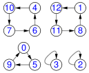
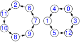
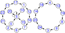
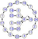
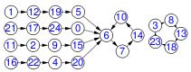
Using the unilateral connected digraph , this section discloses the graph structure of (3) over when (See some examples in Fig. 3). Since there are some zero-divisors in , congruence means ; ; or and , where and . So, solving the equation in is more complicated than that in , which means the period analysis of is much more complex than that given in the previous section. Then, this section divides the whole analysis into three cases: ; ; .
a)
b)
c)
d)
e)
f)
IV-A Graph structure of (3) with
When and or , one has for any , where is the function determined by (3). Thus, the corresponding functional graphs in such cases are trivial. When , , and , Lemma 6 reveals that sequence converges to a constant when its index is sufficiently large, namely there is a self-loop in . Combining the self-loop, Lemma 7 gives the necessary and sufficient conditions for any node whose value is not equal to to be a non-leaf node in . Since when , node of value is a non-leaf node. Then, the in-degree of any non-leaf node is presented in Lemma 8.
Lemma 6.
When , , and , one has for any , where is the function determined by (3), , is the ceiling function, and
Proof.
When , one has , which means for any integer . So, this lemma holds for .
When , by mathematical induction on integer , one can prove
| (17) |
When , since and , Assume that congruence (17) holds for , namely and
| (18) |
where is an integer. It is noted that and are invertible element in for any because and . When , from Eq. (18), one has
Thus, congruence (17) holds for . The above induction completes the proof of congruence (17). From congruence (17), one can know and . It further deduces . ∎
Lemma 7.
When , , and , any node of value is a non-leaf node in if and only if and , where .
Proof.
When a node of value is a non-leaf node in . Then, there exists a node of value such that
| (19) |
From the above equation and
| (20) |
one has . It means . Next, we prove via contradiction. Since and , one can set
| (21) |
where and . If , one has . It yields from Eqs. (19) and (21) that . It further deduces , which contradicts with the definition of . So, .
Lemma 8.
When , , and , the in-degree of any non-leaf node of state value in is if ; otherwise.
Proof.
If , one has for any from Eq. (3). So, the in-degree of the non-leaf node in is .
As shown in Fig. 3a), when , one can know and the self-loop . For edges and , one can calculate when and . So, there is a rule in such case. Then, the similar rule between the self-loop in and any node and its linking node is presented in Lemma 9. Using the Lemma, Proposition 4 discloses how any node evolves to the self-loop.
Lemma 9.
When , , and , one has
| (22) |
where .
Proof.
Proposition 4.
When , , and , any node of value evolves to a unique state of value via a shortest path of length in , where , satisfies , , when , , and .
Proof.
Setting and in Lemma 6, one has , namely . From the definition of , one has is the least non-negative integer such that . Referring to Lemma 9, one can prove
| (24) |
where is an integer. Thus, one can know the value of depends on the value of , where . Combining a partition of the set
the proof is divided into the following two cases:
-
•
: The node of value composes a self-loop.
- •
∎
IV-B Graph structure of (3) with and
As (3) maps any initial state into a fixed value , the structure of the associated connected component is trivial and known. As for any initial state belonging to , (3) composes a permutation when and [42], which means sequence is periodic. So, the graph structure of (3) can be disclosed by studying the period of every sequence starting from every initial state .
From Eq. (10), one has and . It yields that and
| (25) |
Similar to Eq. (13), one has the general term of relation (6) as
| (26) |
For any , let , that is from Eq. (7). It follows from Eq. (26) that
| (27) |
Thus, the period of the sequence equals the smallest integer satisfying congruence (27). Furthermore, Lemma 10 discloses two possible cases on the period of sequence , which is determined by the relation between and .
Lemma 10.
When and , the least period of sequence is
| (28) |
where , , , and .
Proof.
If , one has from Eq. (26). Thus, for any and . If , the proof of this lemma is divided into the following two cases:
- •
- •
∎
From Eqs. (10) and (25), one has . If is a quadratic residue modulo , is reducible over and . It follows from Lemma 10 that there are more than two cases on the lengths of cycles in for any . As shown in Table I, the number of cycles of length remains unchanged with the increase of . Furthermore, Proposition 5 describes the structure of in such case. If is a non-quadratic residue modulo , is irreducible over and , and there is no self-loop in , as shown in Proposition 6.
| 1 | 2 | 10 | |||||
| 1 | 2 | 1 | |||||
| 2 | 2 | 9 | |||||
| 3 | 2 | 24 | 5 | ||||
| 4 | 2 | 24 | 20 | 5 | |||
| 5 | 2 | 24 | 20 | 20 | 5 | ||
| 6 | 2 | 24 | 20 | 20 | 20 | 5 | |
| 7 | 2 | 24 | 20 | 20 | 20 | 20 | 5 |
Proposition 5.
When , , and is a quadratic residue modulo , is composed of connected component , cycles of length , cycles of length , cycles of length two, and two self-loops, where , , and
Proof.
When , one has from (3). So, all states whose values belong to compose connected component .
When , the related analysis is divided into the following two cases:
-
•
: Referring to Lemma 10, one has Since and the definition of , from Eq. (10), which further deduces . It yields from Lemma 1 that So, From Eq. (4), one can get the -adic representation of :
(29) where and for any . Since , one has from Eq. (29). Thus, there are initial states of value such that , and these states compose cycles of length in .
-
•
: One can assume and . The proof of the case and is similar and omitted. When , one has from Lemma 10. It means the state of value composes a self-loop in . When , from the definitions of and , one has and . It further deduces from Lemma 10. Since , one has and
According to Lemma 1 and the above congruence, one can get
(30) If , only the second case of Eq. (30) holds, which means . Referring to Eq. (29), one can get there are initial states of value satisfying and . Thus, all states of value satisfying compose cycles of length two and two self-loops in .
If , the two cases of Eq. (30) hold. From the definition of , one has and . It yields from Eq. (29) that for any , , and for any . So, there are initial states of value satisfying . Then, there are and initial states of value that satisfy the first and second cases of Eq. (30), respectively. Thus, one can know all states of value satisfying compose cycles of length , cycles of length two, and two self-loops in .
∎
When , one has and . As shown in Fig. 3b), is composed of connected component , cycle of length , cycles of length two, and two self-loops. The result is consistent with Proposition 5.
Proposition 6.
When , , and is a non-quadratic residue modulo , is composed of connected component and cycles of length , where .
Proof.
Similar to Proposition 5, one can know all states whose values belong to compose connected component .
Combining the condition of this proposition and , one has is basic irreducible from Lemma 3. It means ring is isomorphic to . So, it from Eq. (4) that and can be expressed as and , where and is an element of order in . For any , since , one has , which yields . It yields from Lemma 10 that . In addition, there are initial states of value such that , which makes up cycles of length in . ∎
IV-C Graph structure of (3) with
When , (3) does not compose a permutation over . Concretely, some states whose values belong to locate on a transient branch in (See Fig. 3d). By analyzing the pre-period and period of the sequence generated by (3) from such nodes, the structure of the corresponding connected components can be disclosed. Equation (26) plays an important role in the process of periodic analysis and is related to . When , may not be a unit, which is different from the case in the previous subsection. From Eq. (10), one has . It deduces is a unit if and only if . The analysis of this subsection is divided according to the condition.
IV-C1
In such case, must be a unit and Eq. (26) still holds for any . The permutation nature of (3) ensures sequence with does not contain any elements in ideal when and . However, when , sequence may contain an element in ideal . Referring to the condition, Lemma 11 gives the explicit expression of the period of the sequence.
Lemma 11.
When and , the pre-period of sequence is not zero if and only if And its least period
| (31) |
where , , , , and
Proof.
Since , one has
| (32) |
from Eq. (26). It yields from congruence (32) that is equivalent to
| (33) |
If , there exists an integer such that from the above congruence, namely . It yields from Lemma 4-ii) that . Hence, . Setting , from Eq. (10), one has
| (34) |
It yields from Eq. (33) that if and only if So, is the smallest integer satisfying , namely . Then, from Lemma 4. Thus, sequence is ultimately periodic and
If and , one has for any integer from congruence (32). Then similar to Lemma 10, one can prove sequence is periodic and
∎
From Fig. 3d), one can see that there exists connected component in . Such structure illustrates there exist some nodes, whose values belong to , located on a transient branch, namely, there are some initial states of value satisfying sequence is ultimately periodic. Lemma 12 gives a set of such initial states of value. Moreover, all nodes whose values belong to the set are leaf-nodes in the functional graph of (3), as shown in Lemma 13.
Lemma 12.
When and , the pre-period and least period of sequence are both equal to , and , where and belongs to
| (35) |
Proof.
For any , one has from Eq. (34). So,
It yields from Lemma 11 that sequence is ultimately periodic and its period is . According to congruence (33) and the above relation, one can know is equivalent to
| (36) |
So, is the smallest integer satisfying , namely . Referring to Lemma 4-ii), one has . It means . From Lemma 11, one has is periodic and its period is . Thus, one can get the pre-period of sequence is . ∎
Lemma 13.
When , the in-degree of any node in set (35) in is zero.
Proof.
For any node of value , assume its in-degree is not zero. Then there exists a node of value such that
From set (35) and , one has . Thus , it contradicts . So, the lemma is proved. ∎
Proposition 7.
When and is a quadratic residue modulo , is composed of connected component , cycles of length , cycles of length , and two self-loops, where and .
Proof.
From the known condition of this proposition, one has the two roots . Depending on the relation between the initial state of value and the two roots, the proof of this proposition is divided into the following three cases:
-
•
: One has . Assume and . When , from Lemma 11. It means the node of value is a self-loop in . When , it follows from Lemma 11 that sequence is periodic and
From Eq. (29), one can know there are initial states of value satisfying . In addition, the case and is similar and omitted. Thus, all states of value satisfying make up cycles of length and two self-loops in .
-
•
: It follows from Lemma 11 that is periodic and
Referring to and the definition of , one can know there are initial states of value satisfying . It means all states satisfying make up cycles of length in .
-
•
: It follows from Lemma 11 that sequence is ultimately periodic and . Let . It follows from Lemma 12 that
So, one can get
(37) From set (35), one can know , which further deduces . From Lemma 13 and set (37), one can know all states belonging to compose a unilateral connected digraph . From the definition of and Eq. (29), one can know there are initial states of value satisfying . Thus, these states compose connected component in .
∎
When , one can calculate , and , , . So, . As shown in Fig. 3e), is composed of connected component , cycles of length four and two self-loops, which is consistent with Proposition 7.
Proposition 8.
When and is a non-quadratic residue modulo , is composed of connected component , cycles of length , where .
Proof.
Similar to Proposition 6, one can know belong to Galois ring not . Thus, and are units for any , which means Depending on whether exists, the proof is divided into the following two cases:
-
•
: It follows that From the definition of and Eq. (29), one can know there are initial states of value satisfying . Thus, these states compose cycles of length in .
-
•
: Similar to Proposition 7, one has and all states of value satisfying compose connected component in .
∎
Note that when is a non-quadratic residue modulo , similar to Eq. (16), one can get , , where and .
IV-C2
In such case, and belong to if is reducible in ; extension ring otherwise. Referring to and Lemma 3, one can know is not a basic irreducible polynomial. It means is not a Galois ring, and its element can be expressed as where [26]. From , one has . So, and
| (38) |
Setting , it yields from that where . Then , where . Then, one can calculate and
| (39) | ||||
Lemma 14 describes if the above equation is congruent to zero modulo , where is a positive integer. Referring to Lemma 14, the pre-period and period of sequence for any is shown in Lemma 15.
Lemma 14.
For any integer , if congruence holds, one has , where and .
Proof.
This lemma is proved via mathematical induction on . When , one has . So, . Assume that this lemma holds for , namely . It means for any . When , from , one has So, . The above induction completes the proof of the lemma. ∎
Lemma 15.
When and , the pre-period of sequence is zero if and only if . And its period
| (40) |
where and .
Proof.
From the definition of sequence and Eq. (38), one has
where and . So,
| (41) |
It means for any if . According to whether the condition holds, the proof is divided into the following two cases:
-
•
: From congruence (41), one can know there exists an integer number such that , namely . It follows from Lemma 4-ii) that must contain some element in . So, . Setting , one can get and by Eq. (41). Thus, is the smallest integer such that , namely . It yields from Lemma 4-ii) that , which deduces . So, is ultimately periodic and .
-
•
: One has for any from Eq. (41), which means that does not contain any element in . So, is the smallest integer that satisfies the congruence , that is
(42) where is an integer. From Eq. (10), one has and is not a unit. It means the general term (26) of relation (6) does not hold. However, Eq. (26) can be transformed into
Multiplying both sides of Eq. (42) by and combining the above equation, one can get . It yields that is equal to the smallest integer that satisfies the congruence
(43) Note that . So, . It yields from Eq. (39) that is the smallest integer satisfying
On the one hand, it is easy to verify that the above congruence holds with , which means . On the other hand, from Lemma 14 and the above congruence holds with , one can get . Thus, .
∎
When , one has from Lemma 15. Setting , one can calculate . From Eq. (38) and the above equation, one has and
| (44) |
When , one has from the above congruence. Moreover, it follows from Lemma 15 that the period of sequence is maximum in this condition. Thus, in this subsection, we only give the graph structure of (3) that can generate the maximum periodic sequence, as shown in Proposition 9, and ignore other cases.
Proposition 9.
When and , is composed of connected component and one cycle of length , where .
Proof.
Similar to Lemma 15, the proof is divided into the following two cases:
- •
-
•
: From the definition of set (35), one has for any , where . Then, similar to the proof of case of Lemma 15, one can prove the pre-period and period of are and . Namely,
Note that there are initial states of value satisfying . Similar to the proof of structure of in Proposition 7, one can prove these states make up connected component in .
∎
V Conclusion
This paper reveals the functional graph of IPRNG over the Galois ring by enumerating distinct sequences with the same least period, generated through the iteration of the generator from every state in the domain. Under every condition on its parameters, the relation between the period of each sequence and the parameters and the initial state of IPRNG is explicitly formulated using the generating polynomial and linear difference equations. The efficacy of the counting method relies on the intricate pattern of the functional graph: there is only one unilateral connected digraph and some cycles with a very small number of different lengths. The paper demonstrates that a non-negligible number of cycles with small periods exist when the parameters are selected improperly. The analysis approach provides a potential solution to the open problem proposed by Solé et al. in [39] regarding the period distribution of the sequence generated by iterating IPRNG over Galois rings . The graph structure over the ring deserves further investigation when is a general composite.
References
- [1] T. Stojanovski and L. Kocarev, “Chaos-based random number generators-part I: analysis,” IEEE Transactions on Circuits and Systems I: Fundamental Theory and Applications, vol. 48, no. 3, pp. 281–288, 2001.
- [2] M. Jessa, “On the quality of random sequences produced with a combined random bit generator,” IEEE Transactions on Computers, vol. 64, no. 3, pp. 791–804, 2015.
- [3] Z. Chang, G. Gong, and Q. Wang, “Cycle structures of a class of cascaded FSRs,” IEEE Transactions on Information Theory, vol. 66, no. 6, pp. 3766–3774, 2019.
- [4] J. Xu, S. Sarkar, L. Hu, H. Wang, and Y. Pan, “New results on modular inversion hidden number problem and inversive congruential generator,” in Advances in Cryptology–Crypto 2019, ser. Lecture Notes in Computer Science, vol. 11692, 2019, pp. 297–321.
- [5] X. Lu, E. Y. Xie, and C. Li, “Periodicity analysis of Logistic map over ring ,” International Journal of Bifurcation and Chaos, vol. 33, no. 5, p. art. no. 2350063, 2023.
- [6] Y. Ma, C. Li, and B. Ou, “Cryptanalysis of an image block encryption algorithm based on chaotic maps,” Journal of Information Security and Applications, vol. 54, p. art. no. 102566, 2020.
- [7] W. Liniger, “On a method by D. H. Lehmer for the generation of pseudo random numbers,” Numerische Mathematik, vol. 3, pp. 265–270, 1961.
- [8] S. K. Park and K. W. Miller, “Random number generators: good ones are hard to find,” Communications of The ACM, vol. 31, p. 1192–1201, 1988.
- [9] HandWiki, “Lehmer random number generator,” https://handwiki.org/wiki/Lehmer_random_number_generator, 2023.
- [10] R. Tausworthe, “Random numbers generated by linear recurrence modulo two,” Mathematics of Computation, vol. 19, pp. 201–201, 1965.
- [11] D. E. Knuth, The art of computer programming, volume 2: seminumerical algorithms, 3rd ed. Boston, MA 02116, USA: Addison-Wesley Professional, 1998.
- [12] L.-Y. Deng, C. Rousseau, and Y. Yuan, “Generalized Lehmer-Tausworthe random number generators,” in Proceedings of the 30th Annual Southeast Regional Conference, 1992, p. 108–115.
- [13] M. Fushimi and S. Tezuka, “The -distribution of generalized feedback shift register pseudorandom numbers,” Communications of The ACM, vol. 26, p. 516–523, 1983.
- [14] L. Afflerbach, “Criteria for the assessment of random number generators,” Journal of Computational and Applied Mathematics, vol. 31, pp. 3–10, 1990.
- [15] V. L. Kurakin, A. S. Kuzmin, A. V. Mikhalev, and A. A. Nechaev, “Linear recurring sequences over rings and modules,” Journal of Mathematical Sciences, vol. 76, no. 6, pp. 2793–2915, 1995.
- [16] X. Zhu and W. Qi, “Compression mappings on primitive sequences over ,” IEEE Transactions on Information Theory, vol. 50, no. 10, pp. 2442–2448, 2004.
- [17] C. Li, X. Zeng, T. Helleseth, C. Li, and L. Hu, “The properties of a class of linear FSRs and their applications to the construction of nonlinear FSRs,” IEEE Transactions on Information Theory, vol. 60, no. 5, pp. 3052–3061, 2014.
- [18] A. Gerosa, R. Bernardini, and S. Pietri, “A fully integrated chaotic system for the generation of truly random numbers,” IEEE Transactions on Circuits and Systems I: Fundamental Theory and Applications, vol. 49, pp. 993–1000, 2002.
- [19] L. Kocarev and G. Jakimoski, “Pseudorandom bits generated by chaotic maps,” IEEE Transactions on Circuits and Systems I: Fundamental Theory and Applications, vol. 50, no. 1, pp. 123–126, 2003.
- [20] T. Addabbo, M. Alioto, A. Fort, S. Rocchi, and V. Vignoli, “Low-hardware complexity PRBGs based on a piecewise-linear chaotic map,” IEEE Transactions on Circuits and Systems II: Express Briefs, vol. 53, no. 5, pp. 329–333, 2006.
- [21] S. M. Ulam and J. von Neumann, “On combination of stochastic and deterministic processes,” Bulletin of the American Mathematical Society, vol. 53, no. 11, p. 1120, 1947.
- [22] T. Addabbo, M. Alioto, A. Fort, S. Rocchi, and V. Vignoli, “The digital Tent map: performance analysis and optimized design as a low-complexity source of pseudorandom bits,” IEEE Transactions on Instrumentation and Measurement, vol. 55, no. 5, pp. 1451–1458, 2006.
- [23] C. Li, B. Feng, S. Li, J. Kurths, and G. Chen, “Dynamic analysis of digital chaotic maps via state-mapping networks,” IEEE Transactions on Circuits and Systems I: Regular Papers, vol. 66, no. 6, pp. 2322–2335, 2019.
- [24] S. C. Phatak and S. S. Rao, “Logistic map: A possible random-number generator,” Physical Review E, vol. 51, no. 4, pp. 3670–3678, 1995.
- [25] C. Li, K. Tan, B. Feng, and J. Lü, “The graph structure of the generalized discrete Arnold’s Cat map,” IEEE Transactions on Computers, vol. 71, no. 2, pp. 364–377, 2022.
- [26] F. Chen, K.-W. Wong, X. Liao, and T. Xiang, “Period distribution of generalized discrete Arnold Cat map for ,” IEEE Transactions on Information Theory, vol. 58, no. 1, pp. 445–452, 2012.
- [27] X. Liao, F. Chen, and K.-w. Wong, “On the security of public-key algorithms based on Chebyshev polynomials over the finite field ,” IEEE Transactions on Computers, vol. 59, no. 10, pp. 1392–1401, 2010.
- [28] F. Chen, X. Liao, T. Xiang, and H. Zheng, “Security analysis of the public key algorithm based on Chebyshev polynomials over the integer ring ,” Information Sciences, vol. 181, no. 22, pp. 5110–5118, 2011.
- [29] T. Addabbo, M. Alioto, A. Fort, A. Pasini, S. Rocchi, and V. Vignoli, “A class of maximum-period nonlinear congruential generators derived from the Rényi chaotic map,” IEEE Transactions on Circuits and Systems I: Regular Papers, vol. 54, no. 4, pp. 816–828, 2007.
- [30] J. Boyar, “Inferring sequences produced by pseudo-random number generators,” Journal of the ACM, vol. 36, p. 129–141, 1989.
- [31] R. Katti, R. Kavasseri, and V. Sai, “Pseudorandom bit generation using coupled congruential generators,” IEEE Transactions on Circuits and Systems II: Express Briefs, vol. 57, no. 3, p. 203–207, 2010.
- [32] A. K. Panda and K. C. Ray, “Modified dual-CLCG method and its VLSI architecture for pseudorandom bit generation,” IEEE Transactions on Circuits and Systems I: Regular Papers, vol. 66, no. 3, p. 989–1002, 2019.
- [33] J. Xu, S. Sarkar, L. Hu, Z. Huang, and L. Peng, “Solving a class of modular polynomial equations and its relation to modular inversion hidden number problem and inversive congruential generator,” Designs, Codes and Cryptography, vol. 86, pp. 1997–2033, 2018.
- [34] J. Eichenauer and J. Lehn, “A non-linear congruential pseudo random number generator,” Statistische Hefte, vol. 27, no. 1, pp. 315–326, 1986.
- [35] H. Leeb and S. Wegenkittl, “Inversive and linear congruential pseudorandom number generators in empirical tests,” ACM Transactions on Modeling and Computer Simulation, vol. 7, no. 2, pp. 272–286, 1997.
- [36] J. Eichenauer-Herrmann and H. Niederreiter, “On the statistical independence of nonlinear congruential pseudorandom numbers,” ACM Transactions on Modeling and Computer Simulation, vol. 4, p. 89–95, 1994.
- [37] J. Eichenauer-Herrmann and H. Grothe, “A new inversive congruential pseudorandom number generator with power of two modulus,” ACM Transactions on Modeling and Computer Simulation, vol. 2, no. 1, pp. 1–11, 1992.
- [38] F. Emmerich, “Average equidistribution and statistical independence properties of digital inversive pseudorandom numbers over parts of the period,” Mathematics of Computation, vol. 71, p. 781–791, 2002.
- [39] P. Solé and D. Zinoviev, “Inversive pseudorandom numbers over Galois rings,” European Journal of Combinatorics, vol. 30, no. 2, pp. 458–467, 2009.
- [40] A. Meidl, Wilfriedand Topuzoğlu, On the Inversive Pseudorandom Number Generator. Heidelberg: Physica-Verlag HD, 2010, pp. 103–125.
- [41] W. S. Chou, “On inversive maximal period polynomials over finite fields,” Applicable Algebra in Engineering, Communication and Computing, vol. 6, no. 4, pp. 245–250, 1995.
- [42] H. Niederreiter and I. Shparlinski, “Exponential sums and the distribution of inversive congruential pseudorandom numbers with prime-power modulus,” Acta Arithmetica, vol. 92, pp. 89–98, 2000.
- [43] H. Niederreiter and A. Winterhof, “Exponential sums and the distribution of inversive congruential pseudorandom numbers with power of two modulus,” International Journal of Number Theory, vol. 01, no. 03, pp. 431–438, 2005.
- [44] J. Eichenauer, J. Lehn, and A. Topuzoǧlu, “A nonlinear congruential pseudorandom number generator with power of two modulus,” Mathematics of Computation, vol. 51, pp. 757–759, 1988.
- [45] J. Eichenauer-Herrmann and A. Topuzoǧlu, “On the period length of congruential pseudorandom number sequences generated by inversions,” Journal of Computational and Applied Mathematics, vol. 31, no. 1, pp. 87–96, 1990.
- [46] W. S. Chou, “The period lengths of inversive pseudorandom vector generations,” Finite Fields and Their Applications, vol. 1, no. 1, pp. 126–132, 1995.
- [47] R. D. Leo and J. A. Yorke, “The graph of the Logistic map is a tower,” Discrete and Continuous Dynamical Systems, vol. 41, no. 11, pp. 5243–5269, 2021.
- [48] C. Qureshi and D. Panario, “The graph structure of Chebyshev polynomials over finite fields and applications,” Designs, Codes and Cryptography, vol. 87, pp. 393–416, 2019.
- [49] D. Panario and L. Reis, “The functional graph of linear maps over finite fields and applications,” Designs, Codes and Cryptography, vol. 87, no. 2-3, pp. 437–453, 2019.
- [50] J. A. Oliveira and F. E. B. Martínez, “Dynamics of polynomial maps over finite fields,” Designs, Codes and Cryptography, vol. 1, no. 1, pp. 1–13, 2023.
- [51] R. Lidl and H. Niederreiter, Introduction to finite fields and their applications, 2nd ed. Cambridge, UK: Cambridge University Press, 1994.
- [52] Z.-X. Wan, Lectures on finite fields and Galois rings. Singapore: World Scientific, 2003.