Solution of the Probabilistic Lambert Problem: Connections with Optimal Mass Transport, Schrödinger Bridge and Reaction-Diffusion PDEs

Abstract

Lambert’s problem concerns with transferring a spacecraft from a given initial to a given terminal position within prescribed flight time via velocity control subject to a gravitational force field. We consider a probabilistic variant of the Lambert problem where the knowledge of the endpoint constraints in position vectors are replaced by the knowledge of their respective joint probability density functions. We show that the Lambert problem with endpoint joint probability density constraints is a generalized optimal mass transport (OMT) problem, thereby connecting this classical astrodynamics problem with a burgeoning area of research in modern stochastic control and stochastic machine learning. This newfound connection allows us to rigorously establish the existence and uniqueness of solution for the probabilistic Lambert problem. The same connection also helps to numerically solve the probabilistic Lambert problem via diffusion regularization, i.e., by leveraging further connection of the OMT with the Schrödinger bridge problem (SBP). This also shows that the probabilistic Lambert problem with additive dynamic process noise is in fact a generalized SBP, and can be solved numerically using the so-called Schrödinger factors, as we do in this work. We explain how the resulting analysis leads to solving a boundary-coupled system of reaction-diffusion PDEs where the nonlinear gravitational potential appears as the reaction rate. We propose novel algorithms for the same, and present illustrative numerical results. Our analysis and the algorithmic framework are nonparametric, i.e., we make neither statistical (e.g., Gaussian, first few moments, mixture or exponential family, finite dimensionality of the sufficient statistic) nor dynamical (e.g., Taylor series) approximations. All our theoretical and computational results are generalizable when the gravitational potential includes higher order zonal and tesseral terms.

Nomenclature

$\mathbb{R}^{d}$  =	Euclidean space of dimension $d$
$\mathbb{R}_{\geq 0}$  =	Set of nonnegative reals
$\mathbb{N}$  =	Set of natural numbers
$\mathbb{E}_{\mathbb{P}}\left[\cdot\right]$  =	Expectation operator with respect to the probability measure $\mathbb{P}$
$|\cdot|$  =	Euclidean magnitude
$\langle\cdot,\cdot\rangle$  =	Euclidean inner product
$\bm{r}=(x,y,z)^{\top}$  =	position in $\mathbb{R}^{3}$
$t$  =	time
$\bm{v}=(v_{x},v_{y},v_{z})^{\top}$  =	velocity in $\mathbb{R}^{3}$
$V$  =	potential
$\mathcal{V}$  =	set of finite energy Markovian velocity control policies
$\mu$  =	the product of the Earth’s gravitational constant and mass, $398600.4415$ km3/s2
$J_{2}$  =	the second zonal harmonic coefficient for the Earth, $1.75553\times 10^{10}$ km5/s2
$\rho$  =	joint probability density function
$\mathcal{P}_{2}\left(\mathbb{R}^{d}\right)$  =	set of probability density functions supported over $\mathbb{R}^{d}$ with finite second moments
$\nabla_{\bm{r}},\nabla_{\bm{r}}\cdot,\Delta_{\bm{r}}$  =	Euclidean gradient, divergence and Laplacian operators with respect to the vector $\bm{r}$
$\varepsilon$  =	diffusive regularization parameter
$\psi$  =	value function
$\widehat{\varphi}_{\varepsilon},\varphi_{\varepsilon}$  =	Schrödinger factors
$C_{c}^{\infty}\left(\mathcal{S}\right)$  =	space of infinitely differentiable functions that are supported on compact subsets of the set $\mathcal{S}$
$C^{1,2}\left(\mathcal{T};\mathcal{S}\right)$  =	space of functions which are once and twice continuously differentiable on $\mathcal{T}$ and $\mathcal{S}$, respectively
$D_{\rm{KL}}\left(\mathbb{P}\parallel\mathbb{Q}\right)$  =	relative entropy a.k.a. Kullback-Leibler divergence between measures $\mathbb{P}$ and $\mathbb{Q}$
$\mathcal{F}\left[\cdot\right],\mathcal{F}^{-1}\left[\cdot\right]$  =	Fourier and inverse Fourier transform
$\mathcal{L}\left[\cdot\right],\mathcal{L}^{-1}\left[\cdot\right]$  =	Laplace and inverse Laplace transform
$(f*g)(\bm{x})$  =	Convolution of functions $f$ and $g$, defined as $\int_{\mathbb{R}^{d}}f(\bm{x}-\bm{y})g(\bm{y}){\rm{d}}\bm{y}=\int_{\mathbb{R}^{d}}f(\bm{y})g(\bm{x}-\bm{y}){\rm{d}}\bm{y}$
$\mathcal{N}\left(\bm{\mu},\bm{\Sigma}\right)$  =	Gaussian probability density function with mean vector $\bm{\mu}$ and covariance matrix $\bm{\Sigma}$
${\rm{diag}}(\bm{x})$  =	Diagonal matrix with main diagonal entries being the elements of the vector $\bm{x}$
a.s., a.e., w.r.t.  =	almost surely, almost everywhere, with respect to

1 Introduction

The classical Lambert problem in orbital mechanics is a finite dimensional two point boundary value problem (TPBVP) over a prescribed time horizon $[t_{0},t_{1}]$ where $t_{0},t_{1}$ are fixed, subject to a two-body gravitational potential force field, and endpoint constraints on the relative position vector. Specifically, for any $t\in[t_{0},t_{1}]$, let $\bm{r}=(x,y,z)^{\top}\in\mathbb{R}^{3}$ be the position and $\bm{v}:=\dot{\bm{r}}\in\mathbb{R}^{3}$ be the velocity of a spacecraft with respect to the Earth centered inertial (ECI) frame. Denote the Euclidean magnitude of the position vector $\bm{r}$ as $|\bm{r}|$.

The classical Lambert’s problem asks to compute a velocity field $\bm{v}=\bm{v}(\bm{r},t)$ subject to the Keplerian equation of motion, endpoint position and hard flight time constraints:

$$\ddot{\bm{r}}=-\nabla_{\bm{r}}V\left(\bm{r}\right),\quad\bm{r}(t=t_{0})=\bm{r}_{0}\>\text{(given)},\quad\bm{r}(t=t_{1})=\bm{r}_{1}\>\text{(given)},$$ (1)

where the nonlinear potential $V(\cdot)$ is bounded, and has typical form:

$$V(\bm{r}):=-\frac{\mu}{|\bm{r}|}-\frac{\mu J_{2}R_{\textrm{Earth}}^{2}}{2|\bm{r}|^{3}}\left(1-\frac{3z^{2}}{|\bm{r}|^{2}}\right),\quad\bm{r}\in[R_{\rm{Earth}},+\infty).$$ (2)

In (2), the parameter $\mu=398600.4415$ km³/s² denotes the product of the Earth’s gravitational constant and mass. The parameter $J_{2}=1.08263\times 10^{-3}$ denotes the (unitless) second zonal harmonic coefficient, which is a measure of the Earth oblateness. The radius of Earth $R_{\textrm{Earth}}=6378.1363$ km.

While we use the potential (2) in numerical simulation (Sec. 6) for specificity, it will be apparent that all our theory and algorithms go through for more general geopotential models [1], i.e., when higher order harmonics (zonal and tesseral terms) are included in $V(\bm{r})$. Specifically, all our results are valid as long as $V(\bm{r})$ is bounded and continuously differentiable, which is indeed the case for all $\bm{r}\in[R_{\rm{Earth}},+\infty)$.

In this work, we consider a probabilistic Lambert problem that softens the endpoint constraints in (1) to

$$\bm{r}(t=t_{0})\sim\rho_{0}\>\text{(given)},\quad\bm{r}(t=t_{1})\sim\rho_{1}\>\text{(given)},$$ (3)

where $\sim$ is a shorthand for “follows the statistical law”. Thus, we allow stochastic uncertainties in the endpoint relative positions, and instead of steering between two given position vectors, we now consider steering between their statistics given by the respective joint probability density functions (PDFs) $\rho_{0},\rho_{1}$. So the probabilistic Lambert problem becomes

$$\underset{\dot{\bm{r}}=\bm{v}(\bm{r},t)}{\text{find}}\quad\bm{v}$$ (4a)

$$\ddot{\bm{r}}=-\nabla_{\bm{r}}V\left(\bm{r}\right),$$ (4b)

$$\bm{r}(t=t_{0})\sim\rho_{0}\>\text{(given)},\quad\bm{r}(t=t_{1})\sim\rho_{1}\>\text{(given)}.$$ (4c)

From an engineering perspective, the PDF $\rho_{0}$ captures initial condition uncertainty (e.g., due to statistical estimation errors). The PDF $\rho_{1}$ on the other hand, encodes desired statistical performance specification, i.e., the allowable terminal condition uncertainty. A small terminal condition uncertainty would imply that $\rho_{1}$ is “tall and skinny” approximating Dirac delta with its Lebesgue mass supported on a small subset of $\mathbb{R}^{3}$. A less stringent terminal uncertainty specification would allow $\rho_{1}$ to have its mass spread over a subset of $\mathbb{R}^{3}$ with larger Lebesgue volume. If problem (4) is feasible, then intuition suggests that a more (resp. less) stringent $\rho_{1}$ specification would result in a more (resp. less) “expensive” control $\bm{v}$ but it is unclear in what sense. As such, (4) is posed as a feasibility problem and even if it admits a unique solution $\bm{v}$ (also unclear why), it is not obvious what optimality guarantee, if any, does that solution usher.

Mathematically, (4) is an infinite dimensional TPBVP since the endpoints $\rho_{0},\rho_{1}$ are elements in the manifold of joint PDFs supported on $\mathbb{R}^{3}$. Solving (4) amounts to computing a PDF-valued curve parameterized by $t\in[t_{0},t_{1}]$ on this infinite dimensional manifold connecting the endpoints $\rho_{0}$ and $\rho_{1}$. Since this manifold is not a vector space, a rigorous solution of this problem requires understanding and systematically leveraging the geometry (e.g., metric structure) in this manifold. The main technical contribution of this work is to clarify how this can be done through a generalization of the theory of optimal mass transport (OMT). We will provide the necessary background for dynamic OMT in Sec. 2.1. Standard references on OMT are [2, 3].

Connecting problem (4) with the OMT allows us to make progress on multiple fronts. First, it allows us to rigorously establish that the solution for (4) is indeed unique. Second, our mathematical development for proving uniqueness reveals that the unique velocity field $\bm{v}$ is indeed optimal in certain minimum effort sense. Third, it allows generalizing (4) for the case when the velocity has additive process noise, i.e., when the controlled ODE

$$\dot{\bm{r}}=\bm{v}(\bm{r},t)$$ (5)

is replaced with the Itô stochastic differential equation (SDE)

$${\rm{d}}\bm{r}=\bm{v}(\bm{r},t)\>{\rm{d}}t+\sqrt{2\varepsilon}\>{\rm{d}}\bm{w}(t),$$ (6)

where $\bm{w}(t)\in\mathbb{R}^{3}$ is the standard Wiener process, and the strength of the process noise $\varepsilon>0$ is not necessarily small. This is of practical interest: the process noise in (6) may result from noisy actuation in velocity command, or from stochastic disturbance in atmospheric drag, solar radiation pressure etc. Our results show that just like problem (4) is a generalized OMT, the corresponding problem with (5) replaced by (6) is a generalized Schrödinger bridge problem (SBP) [4, 5, 6]. We will summarize the necessary background on SBP in Sec. 2.2.

1.1 Related Works

The deterministic Lambert problem has a substantial literature in the guidance-control community – a non-exhaustive list of references includes [7, 8, 9, 10, 11], [12, Ch. 13.4]. A deterministic optimal control reformulation that inspires our development (see Sec. 3.1) is due to [13].

The Lambert problem with probabilistic uncertainty has been investigated before using Taylor expansion [14], using linearization followed by second order statistics (i.e., covariance) mapping [15, 16], using the pushforward mapping of probability measures [17], using polynomial approximation [18], and using neural network and Gaussian process regression [19]. These works consider the endpoint probabilistic uncertainties as in (4c) or some approximants thereof. However, they do not explicitly account for the stochastic dynamics (6). In contrast, recognizing (4) as a generalized OMT naturally leads to a further generalized SBP that precisely corresponds to the controlled stochastic dynamics (6).

The reaction rate appearing in the system of coupled PDEs that we derive has the physical meaning of gravitational potential. It also has a probabilistic interpretation: the rate of killing and creation of probability mass. The recent work [20] also considers an SBP with killing or creation but with unbalanced endpoint marginals, which is not the case for us. While it is possible to convert that unbalanced problem to an equivalent balanced problem, doing so changes the mathematical structure and meaning of the stochastic optimal control problem, see [20, eq. (4.3) and Sec. 5].

1.2 Original Contributions

The present work makes the following novel contributions.

• We establish that the Lambert problem with endpoint joint PDF constraints, i.e., problem (4), is a generalized variant of the OMT problem. The importance of the OMT in dynamics-control problems with probabilistic uncertainties is being recognized across different research communities at a very rapid pace [21, 22, 23, 24, 25, 26, 27, 28, 29, 30]. In this article, we uncover a hitherto unknown link between the OMT and the probabilistic Lambert problem.
  

• Making a precise connection with the OMT allows us to theoretically guarantee existence-uniqueness for the solution of the probabilistic Lambert problem. We accomplish this using two mathematical ingredients: a deterministic optimal control reformulation of the Lambert problem followed by a generalization of the classical dynamic OMT. The former utilizes classical analytical mechanics while the latter relies on a relatively recent development, viz. Figalli’s theory [31] of OMT with cost derived from an action functional.
  

• The connection with OMT also allows for generalization in the sense that the probabilistic Lambert problem with process noise leads to a generalized SBP, which is a stochastic regularization of the OMT. We find that this generalized SBP has an additive state cost which equals to the negative of the gravitational potential. This is a scantily investigated [32, 33] variant of the generalized SBP, and this paper appears to be the first work on the same in engineering literature. Yet, this is precisely the formulation that the probabilistic Lambert problem with process noise leads to. We note that the focus of [32, 33] were to deduce a probabilistic interpretation of such generalized SBPs in the language of the large deviation principle [34]. Our interest here is to actually solve such problems using computational algorithm, which is again a new endeavor.
  

• We show that the additive state cost in the generalized SBP formulation corresponding to the probabilistic Lambert problem with process noise, can be reduced to solving a system of boundary-coupled reaction-diffusion PDEs with state-dependent nonlinear reaction rates. Interestingly, the gravitational potential, with appropriate signs, play the role of these reaction rates. We propose a novel algorithm to numerically solve this system of PDEs and boundary conditions.
  

• We demonstrate that these newfound connections with the OMT and the SBP, allow us to numerically solve the probabilistic Lambert problem using nonparametric computation. In particular, our approach avoids parameterizing the nonlinear dynamics (e.g., using Taylor series) or the statistics (e.g., assuming a finite number of moments such as mean and covariance, parametric families such as Gaussian mixture, exponential family). In this sense, our results are as assumption free as one might hope for.

1.3 Organization of this Paper

In Sec. 2, we provide a brief background on the OMT and the SBP, needed for the technical development that ensues. The subsequent sections are written in a way that a reader, if wishes so, may skip Sec. 2 during the first pass and come back to it as needed. In Sec. 3, we show that accounting for (3) in (1) leads to a generalized version of the OMT problem, which we refer to as the Lambertian optimal mass transport (L-OMT). In Sec. 4, we consider a regularized version of the L-OMT, which we refer to as the Lambertian Schrödinger bridge problem (L-SBP). In Sec. 5, we propose an algorithm to numerically solve the L-SBP. The same algorithm can be used to solve the L-OMT in the small diffusive regularization limit. We provide illustrative numerical results in Sec. 6.

2 Background on OMT and SBP

In this Section, we summarize the classical OMT and SBP background relevant to the technical development that follows. For the Lambert problem of interest, we will need certain generalizations of the classical results summarized here. These generalizations and derivations will be done in situ.

2.1 Optimal Mass Transport (OMT)

Let $\mathcal{P}_{2}\left(\mathbb{R}^{d}\right)$ denote the set of PDFs supported over $\mathbb{R}^{d}$, whose elements have finite second moments, i.e.,

$$\mathcal{P}_{2}\left(\mathbb{R}^{d}\right):=\left\{\rho:\mathbb{R}^{d}\mapsto\mathbb{R}_{\geq 0}\mid\int_{\mathbb{R}^{d}}\rho\mathrm{d}\bm{r}=1,\int_{\mathbb{R}^{d}}|\bm{r}|^{2}\rho\mathrm{d}\bm{r}<\infty\right\}.$$

For $\rho_{0},\rho_{1}\in\mathcal{P}_{2}\left(\mathbb{R}^{d}\right)$, let $\mathcal{P}_{01}$ denote the collection of all PDF-valued trajectories $\rho(\cdot,t)$ continuous in $t\in[t_{0},t_{1}]$, and supported over $\mathbb{R}^{d}$ for each $t\in[t_{0},t_{1}]$, such that $\rho(\cdot,t=t_{0})=\rho_{0},\rho(\cdot,t=t_{1})=\rho_{1}$. Let $\mathcal{V}$ be the set comprising of all Markovian finite energy control policies, i.e.,

$$\mathcal{V}:=\{\bm{v}:\mathbb{R}^{d}\times\left[t_{0},t_{1}\right]\mapsto\mathbb{R}^{d}\mid|\bm{v}|^{2}<\infty\}.$$ (7)

For a given time horizon $[t_{0},t_{1}]$, the dynamic formulation of OMT, introduced by Benamou and Brenier [35], is the variational problem:

$$\underset{(\rho,\bm{v})\in\mathcal{P}_{01}\times\mathcal{V}}{\arg\inf}\int_{t_{0}}^{t_{1}}\int_{\mathbb{R}^{d}}\frac{1}{2}|\bm{v}|^{2}\>\rho(\bm{r},t){\rm{d}}\bm{r}{\rm{d}}t$$ (8a)

$$\qquad\dfrac{\partial\rho}{\partial t}+\nabla_{\bm{r}}\cdot\left(\rho\bm{v}\right)=0,$$ (8b)

$$\qquad\rho(\bm{r},t=t_{0})=\rho_{0},\quad\rho(\bm{r},t=t_{1})=\rho_{1}.$$ (8c)

For details, we refer the readers to [2, Thm. 8.1], [26, Ch. 8].

The objective (8a) seeks to minimize the average control effort $\frac{1}{2}|\bm{v}|^{2}$ with respect to the joint PDF $\rho(\bm{r},t)$. The evolution of the state PDF $\rho(\bm{r},t)$ is governed by the Liouville PDE (8b), which describes the transport of mass under a feasible control policy $\bm{v}\in\mathcal{V}$. The sample path dynamics associated with the Liouville PDE (8b) is the controlled ODE (5); see e.g., [36]. The existence-uniqueness of solution for (8) is guaranteed provided the endpoints $\rho_{0},\rho_{1}\in\mathcal{P}_{2}\left(\mathbb{R}^{d}\right)$.

2.2 Schrödinger Bridge Problem (SBP)

The SBP originated from the works of Erwin Schrödinger [4, 5, 6]. Notably, it predates both the mathematical theory of stochastic processes and the theory of feedback control. Schrödinger’s original motivation for studying this problem was to find a probabilistic interpretation of quantum mechanics. In recent years, SBP with nonlinear prior dynamics [37, 38, 39, 40, 41, 42] have appeared in the literature.

The classical formulation of SBP computes the minimum effort additive control required to steer a given PDF to another given PDF over a specified finite time horizon, subject to a controlled Brownian motion constraint. This leads to a stochastic optimal control problem:

$$\underset{(\rho,\bm{v})\in\mathcal{P}_{01}\times\mathcal{V}}{\arg\inf}\int_{t_{0}}^{t_{1}}\int_{\mathbb{R}^{d}}\frac{1}{2}|\bm{v}|^{2}\>\rho(\bm{r},t)\>{\rm{d}}\bm{r}\>{\rm{d}}t$$ (9a)

$$\qquad\dfrac{\partial\rho}{\partial t}+\nabla_{\bm{r}}\left(\rho\bm{v}\right)=\varepsilon\Delta_{\bm{r}}\rho,\quad\varepsilon>0,$$ (9b)

$$\qquad\rho(\bm{r},t=t_{0})=\rho_{0},\quad\rho(\bm{r},t=t_{1})=\rho_{1}.$$ (9c)

As is the case for (8), the existence-uniqueness of the solution for (9) is guaranteed for $\rho_{0},\rho_{1}\in\mathcal{P}_{2}\left(\mathbb{R}^{d}\right)$. Moreover, the solution of (9) enjoys time-reversibility in the sense that swapping the endpoint data $\rho_{0},\rho_{1}$ results in a solution that is precisely the forward solution run reverse in time over the given time horizon.

When $\varepsilon\downarrow 0$, the SBP (9) reduces to the OMT problem (8) and its solution converges [43, 44, 45] to the solution of (8). Notice that (8b) is the first order Liouville PDE while (9b) is the second order Fokker-Planck-Kolmogorov (FPK) PDE. The macroscopic dynamics (9b) corresponds to the (microscopic) controlled sample path dynamics (6).

3 Lambertian Optimal Mass Transport

The starting point of our development is reformulating (1) as a standard deterministic optimal control problem.

3.1 Formulation

We start with a known result [13, 46] that exactly transforms problem (1) as a standard deterministic optimal control problem with state variable $\bm{r}$ and control variable $\bm{v}$, given by

$$\underset{\bm{v}}{\arg\inf}\quad\displaystyle\int_{t_{0}}^{t_{1}}\left(\dfrac{1}{2}|\bm{v}|^{2}-V(\bm{r})\right){\rm{d}}t$$ (10a)

$$\dot{\bm{r}}=\bm{v},$$ (10b)

$$\bm{r}(t=t_{0})=\bm{r}_{0}\>\text{(given)},\quad\bm{r}(t=t_{1})=\bm{r}_{1}\>\text{(given)}.$$ (10c)

Letting $(\bm{q},\dot{\bm{q}})\equiv(\bm{r},\bm{v})$, this reformulation can be interpreted as the celebrated Hamilton’s principle of least action where the objective in (10a) is an action integral $\int_{t_{0}}^{t_{1}}L(\bm{q},\dot{\bm{q}})\>{\rm{d}}t$ with Lagrangian $L(\bm{q},\dot{\bm{q}}):=T(\dot{\bm{q}})-V(\bm{q})$, the kinetic energy $T(\dot{\bm{q}}):=\frac{1}{2}\langle\dot{\bm{q}},\dot{\bm{q}}\rangle$, and the potential energy $V(\bm{q})$ given by (2). The associated Hamiltonian $H(\bm{q},\dot{\bm{q}})$ defined as the Legendre-Fenchel conjugate of the Lagrangian $L$, equals $H(\bm{q},\dot{\bm{q}})=\langle\frac{\partial L}{\partial\dot{\bm{q}}},\dot{\bm{q}}\rangle-L(\bm{q},\dot{\bm{q}})=T(\dot{\bm{q}})+V(\bm{q})$, the total energy. Consequently, the equations of motion in Hamilton’s canonical variables $(\bm{q},\bm{p}):=(\bm{q},\frac{\partial L}{\partial\dot{\bm{q}}})=(\bm{q},\dot{\bm{q}})$ becomes

$$\dot{\bm{q}}=\dfrac{\partial H}{\partial\bm{p}},\quad\dot{\bm{p}}=-\dfrac{\partial H}{\partial\bm{q}},$$

which is identical to the dynamics $\ddot{\bm{r}}=-\nabla_{\bm{q}}V(\bm{q})$ in (1), as expected.

Replacing the endpoint constraints in (1) with (3) is, therefore, equivalent to modifying the optimal control problem (10) by replacing (10c) with (3). Furthermore, the probabilistic uncertainty in the initial condition $\bm{r}(t=t_{0})\sim\rho_{0}$ is advected by the controlled sample path dynamics (10b) resulting in the joint PDF evolution of the state $\bm{r}(t)$ governed via the Liouville PDE initial value problem (see e.g., [47, 36, 48])

$$\dfrac{\partial\rho}{\partial t}+\nabla_{\bm{r}}\cdot\left(\rho\bm{v}\right)=0,\quad\rho(t=0,\cdot)=\rho_{0}\>\text{(given)},$$ (11)

where $\rho(\bm{r},t)$ denotes the controlled transient joint state PDF for a given control policy $\bm{v}(\bm{r},t)$. The Liouville PDE $\dfrac{\partial\rho}{\partial t}+\nabla_{\bm{r}}\cdot\left(\rho\bm{v}\right)=0$ is the continuity equation signifying the conservation of probability mass over the state space, i.e., $\int_{\mathbb{R}^{3}}\rho(\bm{r},t)\>{\rm{d}}\bm{r}=1$ for all $t\in[t_{0},t_{1}]$. The solution of the Liouville PDE is to be understood in weak sense.

Different feasible control policies $\bm{v}$ in (11) induce different PDF-valued trajectories $\rho(\cdot,t)$ connecting the prescribed endpoint joints $\rho_{0},\rho_{1}\in\mathcal{P}_{2}\left(\mathbb{R}^{3}\right)$. Hence, the objective in (10a) should be averaged w.r.t. the controlled transient joint probability measure $\rho(\bm{r},t)\>{\rm{d}}\bm{r}$, and the resulting functional should be minimized over the pair $(\rho,\bm{v})$. We thus arrive at a generalized OMT formulation

$$\underset{\left(\rho,\bm{v}\right)\in\mathcal{P}_{01}\times\mathcal{V}}{\arg\inf}\quad\displaystyle\int_{t_{0}}^{t_{1}}\int_{\mathbb{R}^{3}}\left(\dfrac{1}{2}|\bm{v}|^{2}-V(\bm{r})\right)\rho(\bm{r},t)\>{\rm{d}}\bm{r}\>{\rm{d}}t$$ (12a)

$$\dfrac{\partial\rho}{\partial t}+\nabla_{\bm{r}}\cdot\left(\rho\bm{v}\right)=0,$$ (12b)

$$\bm{r}(t=t_{0})\sim\rho_{0}\>\text{(given)},\quad\bm{r}(t=t_{1})\sim\rho_{1}\>\text{(given)},$$ (12c)

henceforth referred to as the Lambertian optimal mass transport (L-OMT).

Notice that in the special case when the endpoint joint PDFs are Dirac deltas at some given positions $\bm{r}_{0},\bm{r}_{1}\in\mathbb{R}^{3}$, i.e., $\rho_{0}(\bm{r})=\delta(\bm{r}-\bm{r}_{0}),\rho_{1}(\bm{r})=\delta(\bm{r}-\bm{r}_{1})$, then problem (12) reduces back to (10), or equivalently to (1).

The reader may wonder: what exactly makes problem (12) “generalized”? The answer is the potential $V$, because if $V\equiv 0$ then (12) would be identical to the classical dynamic OMT (8). From a control-theoretic perspective, the problem (12) is an atypical stochastic optimal control problem because it asks to minimize certain total expected “cost-to-go” from a given PDF to another under deadline and controlled dynamics constraints. We next establish the existence-uniqueness of solution for (12).

3.2 Existence and Uniqueness of Solution

To prove the existence-uniqueness result, we start with a definition next.

Definition 1.

(Superlinear function) A function $f\colon\mathbb{R}^{d}\mapsto\mathbb{R}$ is superlinear or 1-coercive, if

$$\lim_{|\bm{x}|\rightarrow\infty}\dfrac{f(\bm{x})}{|\bm{x}|}=+\infty.$$

We now state and prove the following for problem (12).

Theorem 1.

(Existence-uniqueness of solution for L-OMT) Let $\rho_{0},\rho_{1}\in\mathcal{P}_{2}\left(\mathbb{R}^{3}\right)$, and the gravitational potential $V(\cdot)\in(-\infty,0)$ as in (2). Then the minimizing tuple $\left(\rho^{\rm{opt}},\bm{v}^{\rm{opt}}\right)$ for problem (12) exists and is unique.

Proof.

The “cost-to-go” in (12a) is the average of the Lagrangian

$$L(t,\bm{r},\bm{\dot{r}})=\frac{1}{2}|\bm{\dot{r}}|^{2}-V(\bm{r}).$$ (13)

Since $\frac{1}{2}|\cdot|^{2}$ is a strictly convex function, so $L$ is strictly convex in $\bm{\dot{r}}$. We now show that $L$ is also superlinear in $\bm{\dot{r}}$. To see this, notice that

$$\lim_{|\bm{\dot{r}}|\rightarrow\infty}\frac{L}{|\bm{\dot{r}}|}=\lim_{|\bm{\dot{r}}|\rightarrow\infty}\left(\frac{\frac{1}{2}|\bm{\dot{r}}|^{2}-V(\bm{r})}{|\bm{\dot{r}}|}\right)=\left(\lim_{|\bm{\dot{r}}|\rightarrow\infty}\frac{1}{2}|\bm{\dot{r}}|\right)+\left(\lim_{|\bm{\dot{r}}|\rightarrow\infty}\frac{-V(\bm{r})}{|\bm{\dot{r}}|}\right).$$ (14)

The first term $\lim_{|\bm{\dot{r}}|\rightarrow\infty}\frac{1}{2}|\bm{\dot{r}}|=+\infty$. For the second term in (14), $V(\cdot)\in(-\infty,0)$ implies $-V(\bm{r})\in(0,+\infty)$ and thus $\displaystyle\lim_{|\bm{\dot{r}}|\rightarrow\infty}\frac{-V(\bm{r})}{|\bm{\dot{r}}|}=+\infty$. Therefore,

$$\lim_{|\bm{\dot{r}}|\rightarrow\infty}\frac{L}{|\bm{\dot{r}}|}=+\infty.$$

Being strictly convex and superlinear in $\bm{\dot{r}}$, the $L$ in (13) is a weak Tonelli Lagrangian [3, p. 118], [31, Ch. 6.2], which in turn guarantees [31, Thm. 1.4.2] that the pair $\left(\rho^{\rm{opt}},\bm{v}^{\rm{opt}}\right)$ for the generalized OMT problem (12) exists and is unique. ∎

Remark 1.

The proof above only used that the potential $V$ has codomain $(-\infty,0)$; it did not use the specific form (2). Thus, the existence-uniqueness result above applies for generic bounded and continuously differentiable gravitational potentials having codomains in the subsets of $(-\infty,0)$. To explicitly see why the $V$ in (2) is negative, rewrite it as

$$V(\bm{r})=-\dfrac{\mu}{|\bm{r}|}\left(1+\dfrac{J_{2}R_{\rm{Earth}}^{2}}{2|\bm{r}|^{2}}\left(1-\dfrac{3z^{2}}{|\bm{r}|^{2}}\right)\right).$$ (15)

Since $0\leq z^{2}\leq|\bm{r}|^{2}$, we have $-2\leq 1-\frac{3z^{2}}{|\bm{r}|^{2}}\leq 1$. On the other hand, $|\bm{r}|\geq R_{\rm{Earth}}$, which yields

$$\dfrac{J_{2}R_{\rm{Earth}}^{2}}{2|\bm{r}|^{2}}\leq\dfrac{J_{2}R_{\rm{Earth}}^{2}}{2R_{\rm{Earth}}^{2}}\leq\dfrac{J_{2}}{2}<0.0006.$$

Hence,

$$(-2)(0.0006)=-0.0012<\dfrac{J_{2}R_{\rm{Earth}}^{2}}{2|\bm{r}|^{2}}\left(1-\dfrac{3z^{2}}{|\bm{r}|^{2}}\right),\;\text{which gives}\;0<1-0.0012<\left(1+\dfrac{J_{2}R_{\rm{Earth}}^{2}}{2|\bm{r}|^{2}}\left(1-\dfrac{3z^{2}}{|\bm{r}|^{2}}\right)\right).$$ (16)

Combining (15) and (16), we note that $V(\bm{r})<0$.

We next further generalize the L-OMT (12) to allow for stochastic process noise. The resulting problem, as we clarify in Sec. 4, is a generalized version of the SBP (9). Our motivation behind pursuing this generalization is twofold. First, the conditions for optimality that we derive in Sec. 4 helps design nonparametric numerical algorithms, and thereby provably solve the probabilistic Lambert problem in the “small noise” regime. From this perspective, the process noise plays the role of computational regularization. Second, the same theory and algorithm apply when we indeed have (not necessarily small) dynamic process noise due to imperfect actuation, stochastic disturbance in atmospheric drag etc. as mentioned before in Sec. 1.

4 Stochastic Regularization: Lambertian Schrödinger Bridge

4.1 Formulation and Existence-Uniqueness of Solution

For not necessarily small $\varepsilon>0$, and given time horizon $[t_{0},t_{1}]$ as before, we consider a stochastic regularized version of the L-OMT (12):

$$\underset{\left(\rho,\bm{v}\right)\in\mathcal{P}_{01}\times\mathcal{V}}{\arg\inf}\quad\displaystyle\int_{t_{0}}^{t_{1}}\int_{\mathbb{R}^{3}}\left(\dfrac{1}{2}|\bm{v}|^{2}-V(\bm{r})\right)\rho(\bm{r},t)\>{\rm{d}}\bm{r}\>{\rm{d}}t$$ (17a)

$$\dfrac{\partial\rho}{\partial t}+\nabla_{\bm{r}}\cdot\left(\rho\bm{v}\right)=\varepsilon\Delta_{\bm{r}}\rho,$$ (17b)

$$\bm{r}(t=t_{0})\sim\rho_{0}\>\text{(given)},\quad\bm{r}(t=t_{1})\sim\rho_{1}\>\text{(given)},$$ (17c)

which we refer to as the Lambertian Schrödinger Bridge Problem (L-SBP).

The dynamical constraint in (17) differs from (12) by a scaled Laplacian term in the right-hand-side of (17b). The L-SBP (17) generalizes the L-OMT (12) in a similar way the classical SBP (9) generalizes the classical OMT (8).

For arbitrary $\varepsilon>0$, denote the minimizing pair for problem (17) as $\left(\rho_{\varepsilon}^{\rm{opt}},\bm{v}_{\varepsilon}^{\rm{opt}}\right)$ wherein the subscript $\varepsilon$ emphasizes the solution’s dependence on the stochastic regularization parameter $\varepsilon$. We next define the relative entropy a.k.a. Kullback-Leibler divergence, which plays a key role to establish existence-uniqueness for the pair $\left(\rho_{\varepsilon}^{\rm{opt}},\bm{v}_{\varepsilon}^{\rm{opt}}\right)$.

Definition 2.

(Relative entropy a.k.a. Kullback-Leibler divergence) Given two probability measures $\mathbb{P},\mathbb{Q}$ on some measure space $\Omega$, the relative entropy or Kullback-Leibler divergence

$$D_{\rm{KL}}\left(\mathbb{P}\parallel\mathbb{Q}\right):=\mathbb{E}_{\mathbb{P}}\left[\log\dfrac{{\rm{d}}\mathbb{P}}{{\rm{d}}\mathbb{Q}}\right]=\begin{cases}\displaystyle\int_{\Omega}\log\left(\dfrac{{\rm{d}}\mathbb{P}}{{\rm{d}}\mathbb{Q}}\right){\rm{d}}\mathbb{P}&\text{if}\quad\mathbb{P}\ll\mathbb{Q},\\ +\infty&\text{otherwise,}\end{cases}$$ (18)

where $\dfrac{{\rm{d}}\mathbb{P}}{{\rm{d}}\mathbb{Q}}$ denotes the Radon-Nikodym derivative, and $\mathbb{P}\ll\mathbb{Q}$ means “$\mathbb{P}$ is absolutely continuous w.r.t. $\mathbb{Q}$”.

Theorem 2.

(Existence-uniqueness of solution for L-SBP) Let $\rho_{0},\rho_{1}\in\mathcal{P}_{2}\left(\mathbb{R}^{3}\right)$, $\varepsilon>0$, and the gravitational potential $V(\cdot)\in(-\infty,0)$ as in (2). Then the minimizing tuple $\left(\rho_{\varepsilon}^{\rm{opt}},\bm{v}_{\varepsilon}^{\rm{opt}}\right)$ for problem (17) exists and is unique.

Proof.

The main idea behind this proof is to recast (17) as a relative entropy minimization problem w.r.t. a reference Gibbs measure arising from the potential $V$. Here, the role of the reference measure will be played by the Wiener measure on the path space $\Omega:=C\left([t_{0},t_{1}];\mathbb{R}^{3}\right)$, i.e., the space of continuous curves in $\mathbb{R}^{3}$ parameterized by $t\in[t_{0},t_{1}]$. To this end, we follow the developments as in [6] and [32]; see also [49]. We give a self-contained proof here because [6] and [32] are not readily accessible, and also because as written for probabilists, both omit certain technical details. The latter may otherwise pose challenges to theoretically minded engineers–our intended audience–in adapting the core ideas for the case in hand.

Let $\mathcal{M}\left(\Omega\right)$ be the collection of all probability measures on the path space $\Omega$. Recall that (17b) corresponds to the Itô diffusion process (6) where $\bm{v}$ is non-anticipating, i.e., adapted to the filtration generated up until time $t$ for all $t\in[t_{0},t_{1}]$. Let $\mathbb{W}\in\mathcal{M}\left(\Omega\right)$ be a Wiener measure, and consider a measure $\mathbb{P}\in\mathcal{M}\left(\Omega\right)$ generated by the Itô diffusion (6). Using Girsanov’s theorem [50, Thm. 8.6.6], [51, Ch. 3.5], we find

$$\dfrac{{\rm{d}}\mathbb{P}}{{\rm{d}}\mathbb{W}} =\dfrac{{\rm{d}}\mathbb{P}_{0}}{{\rm{d}}\mathbb{W}_{0}}\exp\left(\int_{t_{0}}^{t_{1}}\dfrac{\bm{v}}{\sqrt{2\varepsilon}}{\rm{d}}\bm{w}(t)+\int_{t_{0}}^{t_{1}}\dfrac{1}{2}\dfrac{|\bm{v}|^{2}}{2\varepsilon}{\rm{d}}t\right),\qquad\mathbb{P}\;\>\text{a.s.},$$ (19a)

$$\Leftrightarrow\quad\log\dfrac{{\rm{d}}\mathbb{P}}{{\rm{d}}\mathbb{W}} =\log\dfrac{{\rm{d}}\mathbb{P}_{0}}{{\rm{d}}\mathbb{W}_{0}}+\dfrac{1}{\sqrt{2\varepsilon}}\int_{t_{0}}^{t_{1}}\bm{v}{\rm{d}}\bm{w}(t)+\dfrac{1}{4\varepsilon}\int_{t_{0}}^{t_{1}}|\bm{v}|^{2}{\rm{d}}t,\qquad\mathbb{P}\;\>\text{a.s.},$$ (19b)

where $\mathbb{P}_{0},\mathbb{W}_{0}$ are the distributions of $\bm{r}(t=t_{0})$ under $\mathbb{P}$ and $\mathbb{W}$, respectively.

Since $\bm{v}\in\mathcal{V}$ as defined in (7), we have

$$\mathbb{E}_{\mathbb{P}}\left[\displaystyle\int_{t_{0}}^{t_{1}}|\bm{v}|^{2}{\rm{d}}t\right]<\infty.$$ (20)

So for any $t\geq t_{0}$, the stochastic process

$$\overline{\bm{v}}(t):=\int_{t_{0}}^{t}\bm{v}{\rm{d}}\bm{w}(\tau)$$

is a martingale, and consequently has constant expected value $\mathbb{E}_{\mathbb{P}}\left[\overline{\bm{v}}(t)\right]=\mathbb{E}_{\mathbb{P}}\left[\overline{\bm{v}}(t_{0})\right]=0$. Therefore, applying the expectation operator w.r.t. $\mathbb{P}$ to both sides of (19), we obtain

$$\mathbb{E}_{\mathbb{P}}\left[\log\dfrac{{\rm{d}}\mathbb{P}}{{\rm{d}}\mathbb{Q}}\right]=\mathbb{E}_{\mathbb{P}}\left[\log\dfrac{{\rm{d}}\mathbb{P}_{0}}{{\rm{d}}\mathbb{W}_{0}}\right]+\dfrac{1}{4\varepsilon}\int_{t_{0}}^{t_{1}}\mathbb{E}_{\mathbb{P}}\left[|\bm{v}|^{2}\right]{\rm{d}}t.$$ (21)

Recalling that the potential $V(\cdot)$ is negative and lower bounded (see Remark 1), we next consider the Gibbs measure

$$\dfrac{\exp\left(\dfrac{1}{2\varepsilon}\displaystyle\int_{t_{0}}^{t_{1}}V(\bm{r}){\rm{d}}t\right)\mathbb{W}}{Z}\in\mathcal{M}\left(\Omega\right),\;\text{where the normalization constant}\;Z:=\int_{\Omega}\exp\left(\dfrac{1}{2\varepsilon}\displaystyle\int_{t_{0}}^{t_{1}}V(\bm{r}){\rm{d}}t\right){\rm{d}}\mathbb{W}.$$

By Definition 2, we get

$$D_{\rm{KL}}\left(\mathbb{P}\parallel\dfrac{\exp\left(\dfrac{1}{2\varepsilon}\displaystyle\int_{t_{0}}^{t_{1}}V(\bm{r}){\rm{d}}t\right)\mathbb{W}}{Z}\right) =\log Z+\mathbb{E}_{\mathbb{P}}\left[-\dfrac{1}{2\varepsilon}\displaystyle\int_{t_{0}}^{t_{1}}V(\bm{r}){\rm{d}}t\right]+\mathbb{E}_{\mathbb{P}}\left[\log\dfrac{{\rm{d}}\mathbb{P}}{{\rm{d}}\mathbb{W}}\right]$$

$$=\log Z+\mathbb{E}_{\mathbb{P}}\left[\log\dfrac{{\rm{d}}\mathbb{P}_{0}}{{\rm{d}}\mathbb{W}_{0}}\right]+\dfrac{1}{2\varepsilon}\int_{t_{0}}^{t_{1}}\mathbb{E}_{\mathbb{P}}\left[\dfrac{1}{2}|\bm{v}|^{2}-V(\bm{r})\right]{\rm{d}}t,$$ (22)

where the last equality uses (21).

Let

$$\Pi_{01}:=\bigg{\{}\mathbb{M}\in\mathcal{M}\left(\Omega\right)\mid\mathbb{M}\;\text{has marginal }\;\rho_{i}{\rm{d}}\bm{r}\;\text{at time}\;t_{i}\;\forall i\in\{0,1\},\quad\rho_{0},\rho_{1}\in\mathcal{P}_{2}\left(\mathbb{R}^{3}\right)\bigg{\}}.$$ (23)

Since $\log Z+\mathbb{E}_{\mathbb{P}}\left[\log\dfrac{{\rm{d}}\mathbb{P}_{0}}{{\rm{d}}\mathbb{W}_{0}}\right]$ is constant over $\Pi_{01}$, we conclude from (22) that the stochastic optimal control problem (17) is equivalent to the stochastic calculus of variations problem:

$$\underset{\mathbb{P}\in\Pi_{01}}{\arg\inf}\quad D_{\rm{KL}}\left(\mathbb{P}\parallel\dfrac{\exp\left(\dfrac{1}{2\varepsilon}\displaystyle\int_{t_{0}}^{t_{1}}V(\bm{r}){\rm{d}}t\right)\mathbb{W}}{Z}\right).$$ (24)

From (23), the set $\Pi_{01}$ is closed and convex with non-empty interior. Furthermore, the mapping $\mathbb{P}\mapsto D_{\rm{KL}}\left(\mathbb{P}\parallel\mathbb{Q}\right)$ is strictly convex over $\Pi_{01}$ for a fixed measure $\mathbb{Q}$. Hence there exists unique solution for (24), or equivalently for (17). ∎

Remark 2.

Thanks to the conditional Sanov’s theorem [6, Sec. 4], [52], (24) also shows that the problem (17) enjoys a large deviations principle with rate function $D_{\rm{KL}}\left(\cdot\parallel\frac{\exp\left(\dfrac{1}{2\varepsilon}\int_{t_{0}}^{t_{1}}V(\bm{r}){\rm{d}}t\right)\mathbb{W}}{Z}\right)$. This can be understood intuitively as follows. For $n$ i.i.d. random paths in $\Omega$ with distribution $\mathbb{W}$, when $n$ is large, the more likely paths in $\Pi_{01}$ correspond to those $\mathbb{P}$ which make the objective in (24) small. In particular, for $n\rightarrow\infty$, the path likelihood is asymptotically equivalent to $\exp\left(-n\underset{\mathbb{P}\in\Pi_{01}}{\inf}\>D_{\rm{KL}}\left(\mathbb{P}\parallel\frac{\exp\left(\dfrac{1}{2\varepsilon}\displaystyle\int_{t_{0}}^{t_{1}}V(\bm{r}){\rm{d}}t\right)\mathbb{W}}{Z}\right)\right)$. The most likely path in $\Pi_{01}$ corresponds to the minimizer of (24).

As $\varepsilon\downarrow 0$, clearly the L-SBP (17) reduces to the L-OMT (12). More importantly, as $\varepsilon\downarrow 0$, the solution to (17) converges [44] to the solution of (12), i.e.,

$$\left(\rho_{\varepsilon}^{\rm{opt}},\bm{v}_{\varepsilon}^{\rm{opt}}\right)\xrightarrow{\varepsilon\downarrow 0}\left(\rho^{\rm{opt}},\bm{v}^{\rm{opt}}\right).$$

In the following, we derive the system of equations that solves the optimal pair $\left(\rho_{\varepsilon}^{\rm{opt}},\bm{v}_{\varepsilon}^{\rm{opt}}\right)$.

4.2 Conditions for Optimality

The Proposition 1 next shows that the first order necessary conditions for optimality for the L-SBP (17) takes the form of a coupled system of nonlinear PDEs.

Proposition 1.

(Conditions for optimality for L-SBP) The pair $\left(\rho_{\varepsilon}^{\rm{opt}},\bm{v}_{\varepsilon}^{\rm{opt}}\right)$ solving the L-SBP (17), satisfies the system of coupled PDEs

$$\dfrac{\partial\psi}{\partial t}+\dfrac{1}{2}|\nabla_{\bm{r}}\psi|^{2}+\varepsilon\Delta_{\bm{r}}\psi=-V(\bm{r}),$$ (25a)

$$\dfrac{\partial\rho_{\varepsilon}^{\rm{opt}}}{\partial t}+\nabla_{\bm{r}}\cdot\left(\rho_{\varepsilon}^{\rm{opt}}\nabla_{\bm{r}}\psi\right)=\varepsilon\Delta_{\bm{r}}\rho_{\varepsilon}^{\rm{opt}},$$ (25b)

with boundary conditions

$$\rho_{\varepsilon}^{\rm{opt}}(\bm{r},t=t_{0})=\rho_{0}(\bm{r}),\quad\rho_{\varepsilon}^{\rm{opt}}(\bm{r},t=t_{1})=\rho_{1}(\bm{r}),$$ (26)

where $\psi\in C^{1,2}\left(\mathbb{R}^{3};[t_{0},t_{1}]\right)$, and the optimal control

$$\bm{v}_{\varepsilon}^{\rm{opt}}=\nabla_{\bm{r}}\psi(\bm{r},t).$$ (27)

Proof.

The Lagrangian for the L-SBP (17) is the functional

$$\int_{t_{0}}^{t_{1}}\int_{\mathbb{R}^{3}}\left(\left(\frac{1}{2}|\bm{v}|^{2}-V(\bm{r})\right)\rho(\bm{r},t)+\psi(\bm{r},t)\times\left(\frac{\partial\rho}{\partial t}+\nabla_{\bm{r}}\cdot(\rho\bm{v})-\varepsilon\Delta_{\bm{r}}\rho\right)\right)\>{\rm{d}}\bm{r}\>{\rm{d}}t,$$ (28)

where the Lagrange multiplier $\psi\in C^{1,2}\left(\mathbb{R}^{3};[t_{0},t_{1}]\right)$. The functional (28) depends on the primal-dual variable trio $(\rho,\bm{v},\psi)$. The idea now is to perform unconstrained minimization of (28) over the feasible space $\mathcal{P}_{01}\times\mathcal{V}$.

For the term $\int_{t_{0}}^{t_{1}}\int_{\mathbb{R}^{3}}\psi(\bm{r},t)\frac{\partial\rho}{\partial t}\>{\rm{d}}\bm{r}\>{\rm{d}}t$ in (28), we apply Fubini-Tonelli theorem to switch the order of the integrals, and perform integration by parts w.r.t. $t$, to obtain

$$\int_{t_{0}}^{t_{1}}\int_{\mathbb{R}^{3}}\psi(\bm{r},t)\frac{\partial\rho}{\partial t}\>{\rm{d}}\bm{r}\>{\rm{d}}t=\underbrace{\int_{\mathbb{R}^{3}}\left(\psi(\bm{r},t_{1})\rho_{1}(\bm{r})-\psi(\bm{r},t_{0})\rho_{0}(\bm{r})\right){\rm{d}}\bm{r}}_{\text{constant over }\mathcal{P}_{01}\times\mathcal{V}}-\int_{t_{0}}^{t_{1}}\int_{\mathbb{R}^{3}}\rho(\bm{r},t)\frac{\partial\psi}{\partial t}\>{\rm{d}}\bm{r}\>{\rm{d}}t.$$ (29)

Next, for the term $\int_{t_{0}}^{t_{1}}\int_{\mathbb{R}^{3}}\psi(\bm{r},t)\left(\nabla_{\bm{r}}\cdot(\rho\bm{v})-\varepsilon\Delta_{\bm{r}}\rho\right){\rm{d}}\bm{r}\>{\rm{d}}t$ in (28), integration by parts w.r.t. $\bm{r}$ while assuming the limits at $|\bm{r}|\rightarrow\infty$ are zero, gives

$$\int_{t_{0}}^{t_{1}}\int_{\mathbb{R}^{3}}\psi(\bm{r},t)\left(\nabla_{\bm{r}}\cdot(\rho\bm{v})-\varepsilon\Delta_{\bm{r}}\rho(\bm{r},t)\right){\rm{d}}\bm{r}\>{\rm{d}}t=-\int_{t_{0}}^{t_{1}}\int_{\mathbb{R}^{3}}\langle\nabla_{\bm{r}}\psi,\bm{v}\rangle\rho{\rm{d}}\bm{r}{\rm{d}}t-\varepsilon\int_{t_{0}}^{t_{1}}\int_{\mathbb{R}^{3}}\langle\nabla_{\bm{r}}\rho,\nabla_{\bm{r}}\psi\rangle{\rm{d}}\bm{r}{\rm{d}}t.$$ (30)

For the second integral above, performing integration by parts w.r.t. $\bm{r}$ once more, (30) becomes

$$\int_{t_{0}}^{t_{1}}\int_{\mathbb{R}^{3}}\psi(\bm{r},t)\left(\nabla_{\bm{r}}\cdot(\rho\bm{v})-\varepsilon\Delta_{\bm{r}}\rho(\bm{r},t)\right){\rm{d}}\bm{r}\>{\rm{d}}t=-\int_{t_{0}}^{t_{1}}\int_{\mathbb{R}^{3}}\langle\nabla_{\bm{r}}\psi,\bm{v}\rangle\rho(\bm{r},t){\rm{d}}\bm{r}{\rm{d}}t+\varepsilon\int_{t_{0}}^{t_{1}}\rho(\bm{r},t)\Delta_{\bm{r}}\psi{\rm{d}}\bm{r}\>{\rm{d}}t.$$ (31)

Substituting (29) and (31) back in (28), and dropping the constant term, we arrive at the expression

$$\int_{t_{0}}^{t_{1}}\int_{\mathbb{R}^{3}}\left(\dfrac{1}{2}|\bm{v}|^{2}-V(\bm{r})-\dfrac{\partial\psi}{\partial t}-\langle\nabla_{\bm{r}}\psi,\bm{v}\rangle-\varepsilon\Delta_{\bm{r}}\psi\right)\rho(\bm{r},t)\>{\rm{d}}\bm{r}\>{\rm{d}}t.$$ (32)

Pointwise minimization of (32) w.r.t. $\bm{v}$ for a fixed $\rho\in\mathcal{P}_{01}$, yields the optimal control

$$\bm{v}_{\varepsilon}^{\rm{opt}}=\nabla_{\bm{r}}\psi(\bm{r},t),$$

which is precisely (27). Evaluating (32) at this optimal solution, and equating the resulting expression to zero yields the dynamic programming equation

$$0=\int_{t_{0}}^{t_{1}}\int_{\mathbb{R}^{3}}\left(-\dfrac{1}{2}|\nabla_{\bm{r}}\psi|^{2}-V(\bm{r})-\dfrac{\partial\psi}{\partial t}-\varepsilon\Delta_{\bm{r}}\psi\right)\rho_{\varepsilon}^{\rm{opt}}(\bm{r},t)\>{\rm{d}}\bm{r}\>{\rm{d}}t.$$ (33)

For (33) to hold for arbitrary $\rho\in\mathcal{P}_{01}$, we must have

$$\dfrac{1}{2}|\nabla_{\bm{r}}\psi|^{2}+\dfrac{\partial\psi}{\partial t}+\varepsilon\Delta_{\bm{r}}\psi=-V(\bm{r}),$$ (34)

which is the PDE (25a).

Substituting (27) into the primal feasibility constraint (17b) yields (25b). Finally, the boundary conditions (26) follow from (17c). ∎

For $\varepsilon=0$, the proof above goes through, mutatis mutandis, giving the following for the L-OMT solution $(\rho^{\text{opt}},\bm{v}^{\text{opt}})$ mentioned at the end of Sec. 4.1.

Corollary 3.

(Conditions for optimality for L-OMT) The pair $(\rho^{\rm{opt}},\bm{v}^{\rm{opt}})$ solving the L-OMT (12) , satisfies the system of coupled PDEs

$$\dfrac{\partial\psi}{\partial t}+\dfrac{1}{2}|\nabla_{\bm{r}}\psi|^{2}+V(\bm{r})=0,$$ (35a)

$$\dfrac{\partial\rho^{\rm{opt}}}{\partial t}+\nabla_{\bm{r}}\cdot\left(\rho^{\rm{opt}}\nabla_{\bm{r}}\psi\right)=0,$$ (35b)

with boundary conditions $\rho^{\rm{opt}}(\bm{r},t=t_{0})=\rho_{0}(\bm{r}),\rho^{\rm{opt}}(\bm{r},t=t_{1})=\rho_{1}(\bm{r})$, where $\psi\in C^{1,1}\left(\mathbb{R}^{3};[t_{0},t_{1}]\right)$, and the optimal control $\bm{v}^{\rm{opt}}=\nabla_{\bm{r}}\psi(\bm{r},t)$.

Remark 3.

The second order PDE (25a) is a Hamilton-Jacobi-Bellman (HJB) equation, whereas the second order PDE (25b) is a controlled Fokker-Planck-Kolmogorov (FPK) equation. At the equation level, these two are coupled one way: (25a) only depends on the dual variable $\psi$ while (25b) depends on both $\psi$ and $\rho_{\varepsilon}^{\rm{opt}}$. The boundary conditions (26), however, are only available for the endpoints of the primal variable $\rho_{\varepsilon}^{\rm{opt}}$.

We next focus on finding a solution strategy for the system of coupled nonlinear PDEs (25) with unconventional boundary conditions (26). In the following Theorem 4, we use the Hopf-Cole transform [53, 54] to show that the system (25)-(26) can be exactly converted to a system of linear reaction-diffusion PDEs at the expense of moving the coupling to the boundary conditions. In Sec. 5, we explain how this transformed system is malleable for numerical computation.

Theorem 4.

(Boundary-coupled system of linear reaction-diffusion PDEs) Consider the L-SBP (17) with given $[t_{0},t_{1}]$, $V$, $\varepsilon$, $\rho_{0}$, $\rho_{1}$ as in Theorem 2. Let $\left(\rho^{\mathrm{opt}}_{\varepsilon},\psi\right)$ be the solution of (25)-(26). Consider the Hopf-Cole transform $\left(\rho^{\mathrm{opt}}_{\varepsilon},\psi\right)\mapsto(\widehat{\varphi}_{\varepsilon},\varphi_{\varepsilon})$ defined as

$$\varphi_{\varepsilon} =\exp\left(\frac{\psi}{2\varepsilon}\right),$$ (36a)

$$\widehat{\varphi}_{\varepsilon} =\rho^{\mathrm{opt}}_{\varepsilon}\exp\left(-\frac{\psi}{2\varepsilon}\right).$$ (36b)

Then, the pair $(\widehat{\varphi}_{\varepsilon},\varphi_{\varepsilon})$ called the Schrödinger factors, solve the system of forward and backward linear reaction-diffusion PDEs:

$$\displaystyle\frac{\partial\widehat{\varphi}_{\varepsilon}}{\partial t} =\left(\varepsilon\Delta_{\bm{r}}+\frac{1}{2\varepsilon}V(\bm{r})\right)\widehat{\varphi}_{\varepsilon},$$ (37a)

$$\displaystyle\frac{\partial\varphi_{\varepsilon}}{\partial t} =-\left(\varepsilon\Delta_{\bm{r}}+\frac{1}{2\varepsilon}V(\bm{r})\right)\varphi_{\varepsilon},$$ (37b)

with coupled boundary conditions

$$\widehat{\varphi}_{\varepsilon}(\cdot,t=t_{0})\varphi_{\varepsilon}(\cdot,t=t_{0})=\rho_{0},\quad\widehat{\varphi}_{\varepsilon}(\cdot,t=t_{1})\varphi_{\varepsilon}(\cdot,t=t_{1})=\rho_{1}.$$ (38)

For all $t\in[t_{0},t_{1}]$, the minimizing pair for (17) can be recovered from the Schrödinger factors $(\widehat{\varphi}_{\varepsilon},\varphi_{\varepsilon})$ as

$$\rho_{\varepsilon}^{\rm{opt}}(\cdot,t) =\widehat{\varphi}_{\varepsilon}(\cdot,t)\varphi_{\varepsilon}(\cdot,t),$$ (39a)

$$\bm{v}_{\varepsilon}^{\rm{opt}}(t,\cdot) =2\varepsilon\nabla_{(\cdot)}\log\varphi_{\varepsilon}(\cdot,t).$$ (39b)

Proof.

By definition, $\psi\in C^{1,2}\left([t_{0},t_{1}],\mathbb{R}^{3}\right)$. Being continuous over its entire domain, $\psi$ is bounded. So the mapping (36) is bijective. In particular, both $\widehat{\varphi}_{\varepsilon},\varphi_{\varepsilon}$ are positive over the support of $\rho_{\varepsilon}^{\rm{opt}}$ for all $t\in[t_{0},t_{1}]$.

From (36a),

$$\psi=2\varepsilon\log\varphi_{\varepsilon}.$$ (40)

From (36b), $\widehat{\varphi}_{\varepsilon}=\rho^{\mathrm{opt}}_{\varepsilon}\exp(-\log(\varphi_{\varepsilon}))$, which immediately gives (39a). Substituting (40) in (27) gives (39b). Since (39a) holds for all $t\in[t_{0},t_{1}]$, so combining (26) and (39a) yields (38). All that remains is to derive (37).

Substituting (40) in (25a), we get

$$2\varepsilon^{2}\bigg{|}\frac{1}{\varphi_{\varepsilon}}\nabla_{\bm{r}}\varphi_{\varepsilon}\bigg{|}^{2}+2\varepsilon\frac{1}{\varphi_{\varepsilon}}\dfrac{\partial\varphi_{\varepsilon}}{\partial t}+\varepsilon\Delta_{\bm{r}}(2\varepsilon\log\varphi_{\varepsilon})=-V(\bm{r}).$$ (41)

Since $\Delta_{\bm{r}}(2\varepsilon\log\varphi_{\varepsilon})=2\varepsilon\nabla_{\bm{r}}\nabla_{\bm{r}}\log\varphi_{\varepsilon}=2\varepsilon\nabla_{\bm{r}}\left(\frac{1}{\varphi_{\varepsilon}}\nabla_{\bm{r}}\varphi\right)=2\varepsilon\left(-\frac{1}{\varphi_{\varepsilon}^{2}}\langle\nabla_{\bm{r}}\varphi_{\varepsilon},\nabla_{\bm{r}}\varphi_{\varepsilon}\rangle+\frac{1}{\varphi_{\varepsilon}}\Delta_{\bm{r}}\varphi_{\varepsilon}\right)$, (41) simplifies to

$$2\varepsilon^{2}\bigg{|}\frac{1}{\varphi_{\varepsilon}}\nabla_{\bm{r}}\varphi_{\varepsilon}\bigg{|}^{2}+2\varepsilon\frac{1}{\varphi_{\varepsilon}}\dfrac{\partial\varphi_{\varepsilon}}{\partial t}+2\varepsilon^{2}\left(-\frac{1}{\varphi_{\varepsilon}^{2}}\langle\nabla_{\bm{r}}\varphi_{\varepsilon},\nabla_{\bm{r}}\varphi_{\varepsilon}\rangle+\frac{1}{\varphi_{\varepsilon}}\Delta_{\bm{r}}\varphi_{\varepsilon}\right)=-V(\bm{r}),$$

$$\Leftrightarrow\quad 2\varepsilon\frac{1}{\varphi_{\varepsilon}}\dfrac{\partial\varphi_{\varepsilon}}{\partial t}+2\varepsilon^{2}\left(\frac{1}{\varphi_{\varepsilon}}\Delta_{\bm{r}}\varphi\right)=-V(\bm{r}).$$ (42)

Rearranging (42), we obtain (37b).

Next, substituting (39a) and (40) in (25b), we find

$$\dfrac{\partial}{\partial t}\left(\widehat{\varphi}_{\varepsilon}\varphi\right)+\nabla_{\bm{r}}\cdot\left(\widehat{\varphi}_{\varepsilon}\varphi_{\varepsilon}\nabla_{\bm{r}}(2\varepsilon\log\varphi_{\varepsilon})\right)=\varepsilon\Delta_{\bm{r}}\left(\widehat{\varphi}_{\varepsilon}\varphi_{\varepsilon}\right),$$

$$\Leftrightarrow\quad \varphi_{\varepsilon}\dfrac{\partial\widehat{\varphi}_{\varepsilon}}{\partial t}+\widehat{\varphi}_{\varepsilon}\dfrac{\partial\varphi_{\varepsilon}}{\partial t}+\nabla_{\bm{r}}\cdot\left(2\varepsilon\widehat{\varphi}_{\varepsilon}\varphi_{\varepsilon}\frac{1}{\varphi_{\varepsilon}}\nabla_{\bm{r}}\varphi_{\varepsilon}\right)=\varepsilon\left(\varphi_{\varepsilon}\Delta_{\bm{r}}\widehat{\varphi}_{\varepsilon}+2\langle\nabla_{\bm{r}}\widehat{\varphi}_{\varepsilon},\nabla_{\bm{r}}\varphi_{\varepsilon}\rangle+\widehat{\varphi}_{\varepsilon}\Delta_{\bm{r}}\varphi_{\varepsilon}\right),$$ (43)

where the right-hand-side of (43) used the identity $\Delta(fg)=f\Delta g+2\langle\nabla f,\nabla g\rangle+g\Delta f$ for twice differentiable $f,g$.

We expand the term $\nabla_{\bm{r}}\cdot\left(2\varepsilon\widehat{\varphi}_{\varepsilon}\varphi_{\varepsilon}\frac{1}{\varphi_{\varepsilon}}\nabla_{\bm{r}}\varphi_{\varepsilon}\right)$ appearing in the left-hand-side of (43) as

$$\nabla_{\bm{r}}\cdot\left(2\varepsilon\widehat{\varphi}_{\varepsilon}\varphi_{\varepsilon}\frac{1}{\varphi_{\varepsilon}}\nabla_{\bm{r}}\varphi_{\varepsilon}\right)=2\varepsilon\langle\nabla_{\bm{r}}\widehat{\varphi}_{\varepsilon},\nabla_{\bm{r}}\varphi_{\varepsilon}\rangle+2\varepsilon\widehat{\varphi}_{\varepsilon}\Delta_{\bm{r}}\varphi_{\varepsilon},$$

and therefore, (43) simplifies to

$$\varphi_{\varepsilon}\dfrac{\partial\widehat{\varphi}_{\varepsilon}}{\partial t}+\widehat{\varphi}_{\varepsilon}\dfrac{\partial\varphi_{\varepsilon}}{\partial t}+\varepsilon\widehat{\varphi}_{\varepsilon}\Delta_{\bm{r}}\varphi_{\varepsilon}=\varepsilon\varphi_{\varepsilon}\Delta_{\bm{r}}\widehat{\varphi}_{\varepsilon},$$

$$\Leftrightarrow\quad \varphi_{\varepsilon}\dfrac{\partial\widehat{\varphi}_{\varepsilon}}{\partial t}+\widehat{\varphi}_{\varepsilon}\left(\dfrac{\partial\varphi_{\varepsilon}}{\partial t}+\varepsilon\Delta_{\bm{r}}\varphi_{\varepsilon}\right)=\varepsilon\varphi_{\varepsilon}\Delta_{\bm{r}}\widehat{\varphi}_{\varepsilon},$$

$$\Leftrightarrow\quad \varphi_{\varepsilon}\dfrac{\partial\widehat{\varphi}_{\varepsilon}}{\partial t}+\widehat{\varphi}_{\varepsilon}\left(-\frac{1}{2\varepsilon}V(\bm{r})\varphi_{\varepsilon}\right)=\varepsilon\varphi_{\varepsilon}\Delta_{\bm{r}}\widehat{\varphi}_{\varepsilon},$$ (44)

where the last line’s left-hand-side used the already derived PDE (37b). Rearranging (44), we arrive at (37a). This completes the proof. ∎

Remark 4.

The derived (37)-(38) is a boundary coupled system of linear reaction-diffusion PDEs. Specifically, (37a) (resp. (37b)) is a forward-in-time (resp. backward-in-time) reaction-diffusion PDE with state-dependent reaction rate $V(\bm{r})$. Once this PDE system for the Schrödinger factors is solved, the optimally controlled joint PDF and the optimal control can then be computed using (39). In Sec. 5, we will outline how to solve (37)-(38). Notice that the special case $V\equiv 0$ corresponding to the classical SBP in Sec. 2.2, reduces (37) to a system of forward-backward heat PDEs.

Remark 5.

The derived system (37)-(38) has the following probabilistic interpretation. This is a system of forward-backward diffusions where individual points in the state space $\mathbb{R}^{3}$ move forward and reverse in time according to Brownian motion with variance $2\varepsilon$, together with killing or creation of probability mass at rate $V(\bm{r})$. Thus, $V(\bm{r})$ in (37a) is position-dependent killing rate (recall $V$ is negative). Likewise, $V(\bm{r})$ in (37b) is position-dependent creation rate. The boundary conditions (38) ensure that the total probability mass remains balanced. For gravitational potentials such as (2), the killing and creation rates are small (resp. large) when $|\bm{r}|$ is large (resp. small).

5 Algorithm

In this Section, we start by outlining our overall approach (Sec. 5.1) to numerically solve the system (37)-(38). We then provide some details (Sec. 5.2-5.3) needed to carry out that overall approach.

5.1 Overall Approach

Our high level idea is to solve (37)-(38) via a recursive algorithm. Specifically, suppose that we have access to initial value problem (IVP) solvers for the PDEs (37). However, the endpoint Schrödinger factors

$$\widehat{\varphi}_{\varepsilon,0}(\cdot):=\widehat{\varphi}_{\varepsilon}(\cdot,t=t_{0}),\quad\varphi_{\varepsilon,1}(\cdot):=\varphi_{\varepsilon}(\cdot,t=t_{1}),$$ (45)

in (38) are not known. The proposed recursive algorithm starts with making an initial (everywhere positive) guess for the endpoint factor $\widehat{\varphi}_{\varepsilon,0}$, and with this initial guess, we integrate (37a) forward in time using the IVP solver to predict $\widehat{\varphi}_{\varepsilon}(\cdot,t=t_{1})$. Then, applying the known boundary condition (38) at $t=t_{1}$ generates a guess for $\varphi_{\varepsilon,1}(\cdot)$, which we use to integrate (37b) backward in time to predict $\varphi_{\varepsilon}(\cdot,t=t_{0})$. Subsequently, applying the known boundary condition (38) at $t=t_{0}$ generates a new guess for $\varphi_{\varepsilon,0}(\cdot)$, thereby completing one pass of the proposed recursion. This process is then repeated as shown in Fig. 1.

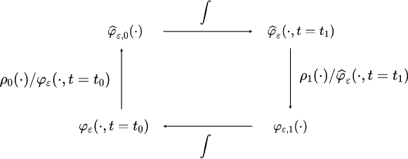
Figure 1: Fixed point recursion over the endpoint Schrödinger factor pair $(\widehat{\varphi}_{\varepsilon,0},\varphi_{\varepsilon,1})$ to solve the boundary-coupled system of PDEs (37)-(38). The arrows with integrals denote marching the respective IVP solution over time.

Notice that in practical numerical simulations, $\rho_{0},\rho_{1}$ are compactly supported, which is indeed a sufficient condition for our standing assumption $\rho_{0},\rho_{1}\in\mathcal{P}_{2}\left(\mathbb{R}^{3}\right)$. That the above-mentioned recursion for compactly supported endpoint data, has guaranteed linear convergence w.r.t. the Hilbert’s projective metric [55, 56, 57], has been proved in various degrees of generalities in the literature, see e.g., [58, Sec. III]. For references related to this contractive fixed point recursion, see e.g., [59, 60, 41, 40, 61].

We note that a convergent solution for the Schrödinger factor recursion determines these factors in a projectivized unique sense, i.e., the recursion finds $\left(\kappa\widehat{\varphi}_{\varepsilon,0}(\cdot),\frac{1}{\kappa}\varphi_{\varepsilon,1}(\cdot)\right)$, and thus $\left(\kappa\widehat{\varphi}_{\varepsilon}(\cdot,t),\frac{1}{\kappa}\varphi_{\varepsilon}(\cdot,t)\right)$ for $t\in[t_{0},t_{1}]$, up to an arbitrary constant $\kappa>0$. The product of these factors is the optimally controlled joint PDF $\rho^{\text{opt}}_{\varepsilon}(\cdot,t)$, which is unique in the usual sense.

For the unknown function pair (45), the recursion proposed above effectively solves a Schrödinger system, i.e., a system of nonlinear integral equations

$$\rho_{0}(\bm{r})=\widehat{\varphi}_{\varepsilon,0}(\bm{r})\int_{\mathbb{R}^{3}}q_{\varepsilon}(t_{0},\bm{r},t_{1},\bm{y})\varphi_{\varepsilon,1}(\bm{y})\mathrm{d}\bm{y},$$ (46a)

$$\rho_{1}(\bm{r})=\varphi_{\varepsilon,1}(\bm{r})\int_{\mathbb{R}^{3}}q_{\varepsilon}(t_{0},\bm{y},t_{1},\bm{r})\widehat{\varphi}_{\varepsilon,0}(\bm{y})\mathrm{d}\bm{y},$$ (46b)

where $q_{\varepsilon}$ is the (uncontrolled) Markov kernel associated with (37). In our setting, evaluation of the integrals in (46) are performed by the IVP solvers for (37). For the readers’ convenience, we summarize the steps of our proposed algorithm.

Step 1. Make an initial guess for $\widehat{\varphi}_{\varepsilon,0}$ that is everywhere positive.

Step 2. Use the $\widehat{\varphi}_{\varepsilon,0}$ from Step 1 to integrate (37a) from $t=t_{0}$ to $t=t_{1}$, to determine $\widehat{\varphi}_{\varepsilon}(\cdot,t=t_{1})$.

Step 3. Set $\varphi_{\varepsilon,1}=\rho_{1}(\cdot)/\widehat{\varphi}_{\varepsilon}(\cdot,t=t_{1})$ by enforcing (38) at $t=t_{1}$.

Step 4. Use the $\varphi_{\varepsilon,1}$ from Step 3 to integrate (37b) from $t=t_{1}$ to $t=t_{0}$ to determine $\varphi_{\varepsilon}(\cdot,t=t_{0})$.

Step 5. Redefine $\widehat{\varphi}_{\varepsilon,0}=\rho_{0}/\varphi_{\varepsilon}(\cdot,t=t_{0})$ by enforcing (38) at $t=t_{0}$.

Step 6. Repeat Steps 2-5 until the pair $(\widehat{\varphi}_{\varepsilon,0}(\cdot),\varphi_{\varepsilon,1}(\cdot))$ has converged up to a desired numerical tolerance.

Step 7. With the converged endpoint factors $\widehat{\varphi}_{\varepsilon,0}(\cdot),\varphi_{\varepsilon,1}(\cdot)$ from Step 6, compute the transient factors $\widehat{\varphi}_{\varepsilon}(\cdot,t),\varphi_{\varepsilon}(\cdot,t)$ at desired $t\in[t_{0},t_{1}]$ using the IVP solver for (37a) and (37b).

Step 8. Use (39) to return the optimal solution $\left(\rho_{\varepsilon}^{\rm{opt}},\bm{v}_{\varepsilon}^{\rm{opt}}\right)$ for the L-SBP.

In describing our overall approach, so far we presumed the availability of an IVP solver for (37). We next detail certain integral representation formula for the solution of the IVP for (37). This in turn facilitates the implementation of such an IVP solver.

5.2 Integral Representation for the Schrödinger Factors

We need the following Lemma 1. Its proof uses few Fourier transform results given in Appendix A. The proof is deferred to Appendix B.

Lemma 1.

(Integral representation for the solution of linear reaction-diffusion PDE IVP with state-dependent reaction rate) For $t\in[t_{0},\infty)$, the solution of the reaction-diffusion PDE IVP

$$\dfrac{\partial u}{\partial t}=a\Delta_{\bm{x}}u+b(\bm{x})u,\quad\bm{x}\in\mathbb{R}^{d},\quad u(\bm{x},t=t_{0})=u_{0}(\bm{x})\;\text{given},$$ (47)

where the constant $a>0$ and the function $b(\bm{x})$ is sufficiently smooth a.e., satisfies

$$u(\bm{x},t)=\underbrace{\dfrac{1}{\sqrt{\left(4\pi at\right)^{d}}}\displaystyle\int_{\mathbb{R}^{d}}\exp\left(-\dfrac{|\bm{x}-\bm{y}|^{2}}{4at}\right)u_{0}(\bm{y}){\rm{d}}\bm{y}}_{\text{term 1}}+\underbrace{\displaystyle\int_{t_{0}}^{t}\dfrac{1}{\sqrt{\left(4\pi a(t-\tau)\right)^{d}}}\displaystyle\int_{\mathbb{R}^{d}}\exp\left(-\dfrac{|\bm{x}-\bm{y}|^{2}}{4a(t-\tau)}\right)b(\bm{y})u(\bm{y},\tau)\>{\rm{d}}\bm{y}\>{\rm{d}}\tau}_{\text{term 2}}.$$ (48)

Remark 6.

The right-hand-side of (48) is a sum of two terms: term 1 is the solution of the heat PDE IVP accounting for the initial condition $u_{0}(\cdot)$; term 2 captures the effect of the reaction rate $b(\cdot)$. We can view (48) as a Fredholm integral equation of second kind.

Specializing (48) with $n=3$ for the IVP involving (37a), we get an integral representation formula

$$\widehat{\varphi}_{\varepsilon}(\bm{r},t)=\frac{1}{\sqrt{(4\pi\varepsilon t)^{3}}}\int_{\mathbb{R}^{3}}\textrm{exp}\left(-\frac{|\bm{r}-\tilde{\bm{r}}|^{2}}{4\varepsilon t}\right)\widehat{\varphi}_{\varepsilon,0}(\tilde{\bm{r}})\>{\rm{d}}\tilde{\bm{r}}+\int_{t_{0}}^{t}\frac{1}{2\varepsilon\sqrt{(4\pi\varepsilon(t-\tau))^{3}}}\int_{\mathbb{R}^{3}}\textrm{exp}\left(-\frac{|\bm{r}-\tilde{\bm{r}}|^{2}}{4\varepsilon(t-\tau)}\right)V(\tilde{\bm{r}})\widehat{\varphi}_{\varepsilon}(\tilde{\bm{r}},\tau)\>{\rm{d}}\tilde{\bm{r}}\>{\rm{d}}\tau.$$ (49)

To complete Step 2 of our algorithm, we approximate (49) as further detailed in Sec. 5.3.

Additionally, consider a change of time variable $t\mapsto\bar{t}:=t_{0}+t_{1}-t$. When the physical time $t\in[t_{1},t_{0}]$ flows backward, then the transformed time $\bar{t}\in[t_{0},t_{1}]$ flows forward. This allows the IVP involving (37b) to be rewritten as

$$\frac{\partial\bar{\varphi}_{\varepsilon}}{\partial\bar{t}}\left(\bm{r},\bar{t}\right)=\left(\varepsilon\Delta_{\bm{r}}+\frac{1}{2\varepsilon}V(\bm{r})\right)\bar{\varphi}_{\varepsilon}(\bm{r},\bar{t}),\qquad\bar{\varphi}_{\varepsilon}\left(\bm{r},\bar{t}=t_{0}\right)=\varphi_{\varepsilon,1}.$$ (50)

From the solution of (50), we recover $\varphi_{\varepsilon}(\bm{r},t)=\bar{\varphi}_{\varepsilon}(\bm{r},t_{0}+t_{1}-t)$. Thus, for our algorithm in Sec. 5.1, we can reuse the same IVP solver from Step 2 to complete Step 4.

5.3 Left Riemann Sum Approximation

For the numerical implementation of the IVP solver mentioned before, we now explain how the right-hand-side of (49), specifically its second summand, can be approximated via left Riemann sum. Recall that (cf. Remark 6) the first summand in the right-hand-side of (49) is the well-known solution of the heat equation, denoted as $\widehat{\varphi}_{\text{heat}}(\bm{r},t)$, which can be implemented by direct matrix-vector multiplication over a computational domain. In particular, we uniformly discretize a hyper-rectangular computational domain $[x_{\min},x_{\max}]\times[y_{\min},y_{\max}]\times[z_{\min},z_{\max}]\times[t_{0},t_{1}]\subset\mathbb{R}^{3}\times[t_{0},t_{1}]$. Along the space-time dimensions, we use constant step sizes $\Delta x,\Delta y,\Delta z$, $\Delta t$ for $N_{x}$, $N_{y}$, $N_{z}$, $N_{t}$ steps, respectively.

We assign $\widehat{\varphi}_{\varepsilon}(\bm{r},t)\leftarrow\widehat{\varphi}_{\varepsilon,0}$ for $t\in[t_{0},t_{0}+\Delta t)$, and approximate the second term of (49) as

$$\widehat{\varphi}_{\textrm{left}}(\bm{r},t=t_{0}+\Delta t)=\frac{1}{2\varepsilon\sqrt{(4\pi\varepsilon(\Delta t))^{3}}}\sum_{m=0}^{N_{x}}\left(\sum_{n=0}^{N_{y}}\left(\sum_{j=0}^{N_{z}}\textrm{exp}\left(-\frac{|\bm{r}-\widetilde{\bm{r}}_{(m,n,j)}|^{2}}{4\varepsilon\Delta t}\right)V(\widetilde{\bm{r}}_{(m,n,j)})\widehat{\varphi}_{\varepsilon,0}(\widetilde{\bm{r}}_{(m,n,j)})\right)\right)\Delta x\Delta y\Delta z\Delta t,$$ (51)

where $\widetilde{\bm{r}}_{(m,n,j)}:=[x_{\min}+m\Delta x,y_{\min}+n\Delta y,z_{\min}+j\Delta z]^{\top}$ and the tuple $(m,n,j)\in\{0,1,\ldots,N_{x}\}\times\{0,1,\ldots,N_{y}\}\times\{0,1,\ldots,N_{z}\}$. We thus get

$$\widehat{\varphi}_{\varepsilon}(\bm{r},t=t_{0}+\Delta t)\approx\widehat{\varphi}_{\varepsilon,\textrm{approx}}(\bm{r},t=t_{0}+\Delta t)=\widehat{\varphi}_{\textrm{heat}}(\bm{r},t=t_{0}+\Delta t)+\widehat{\varphi}_{\textrm{left}}(\bm{r},t=t_{0}+\Delta t).$$

For $k\in\{1,\ldots,N_{t}\}$, we construct a recursive formula for $\widehat{\varphi}_{\varepsilon,\textrm{approx}}(\bm{r},t=t_{0}+k\Delta t)$ using $\widehat{\varphi}_{\varepsilon,\textrm{approx}}(\bm{r},t=t_{0}+q\Delta t)$ $\forall\{q\in\mathbb{N}\cup\{0\}\mid q<k\}$. We approximate $\widehat{\varphi}_{\varepsilon}(\bm{r},t)\approx\widehat{\varphi}_{\varepsilon,\textrm{approx}}(\bm{r},t=t_{0}+q\Delta t)$ for $t\in[t_{0}+q\Delta t,t_{0}+(q+1)\Delta t)$. To evaluate the second term of (49), we integrate over each interval $[t_{0}+q\Delta t,t_{0}+(q+1)\Delta t)$ using triple summation, as in the calculation of $\widehat{\varphi}_{\textrm{left}}(\bm{r},t=t_{0}+\Delta t)$. This yields a recursive formula

$$\widehat{\varphi}_{\textrm{left}}(\bm{r},t_{0}+k\Delta t)=\sum_{q=0}^{k-1}\left(\frac{1}{2\varepsilon\sqrt{(4\pi\varepsilon(k-q)\Delta t)^{3}}}\sum_{m=0}^{N_{x}}\left(\sum_{n=0}^{N_{y}}\left(\sum_{j=0}^{N_{z}}\textrm{exp}\left(-\frac{|\bm{r}-\widetilde{\bm{r}}_{(m,n,j)}|^{2}}{4\varepsilon(k-q)\Delta t}\right)\right.\right.\right.$$

$$\qquad\qquad\qquad\qquad\qquad\qquad\qquad\qquad\left.\left.\left.V(\widetilde{\bm{r}}_{(m,n,j)})\widehat{\varphi}_{\varepsilon,\textrm{approx}}(\widetilde{\bm{r}}_{(m,n,j)},t_{0}+q\Delta t)\right)\right)\right)\Delta x\Delta y\Delta z\Delta t.$$ (52)

Notice that specializing (52) for $k=1$ recovers (51), as expected.

As earlier, we set $\widehat{\varphi}_{\varepsilon,\textrm{approx}}(\bm{r},t=t_{0}+k\Delta t)=\widehat{\varphi}_{\textrm{heat}}(\bm{r},t=t_{0}+k\Delta t)+\widehat{\varphi}_{\textrm{left}}(\bm{r},t=t_{0}+k\Delta t)$. Applying this result, we complete Step 2 of our algorithm in Sec. 5.1 using

$$\widehat{\varphi}_{\varepsilon}(\bm{r},t_{1})\approx\widehat{\varphi}_{\varepsilon,\textrm{approx}}(\bm{r},t_{1})=\widehat{\varphi}_{\textrm{heat}}(\bm{r},t_{1})+\widehat{\varphi}_{\textrm{left}}(\bm{r},t_{1}).$$

Likewise, Step 4 of our algorithm in Sec. 5.1 is completed via this left Riemann sum approximation in conjunction with the change of variable $\bar{t}=t_{0}+t_{1}-t$ discussed in Sec. 5.2.

Remark 7.

An alternative way to numerically solve the IVPs associated with (37) is to use the Feynman-Kac path integral [50, Ch. 8.2], [62], [63, Ch. 3.3], which was recently used to solve a class of SBPs [42]. Note that this also requires a function approximation oracle.

6 Numerical Results

We illustrate our proposed algorithm for solving the L-SBP in a low Earth orbit (LEO) transfer case study as in Kim and Park [46] and Curtis [64]. Specifically, we consider stochastic transfer of a spacecraft from initial mean position $[5000,10000,2100]^{\top}$ km to a final mean position $[-14600,2500,7000]^{\top}$ km in ECI coordinates for a fixed flight time horizon $[t_{0},t_{1}]=[0,1\>\text{hour}]$.

For numerical conditioning, we re-scale the variables as $\bm{r}^{\prime}:=\bm{r}/R$, $t^{\prime}:=t/T$, where the normalization constants $R=6600$ km and $T=5399$ s. In these re-scaled coordinates, the potential (2) becomes

$$\overline{V}(\bm{r}^{\prime})=-\frac{\mu_{\textrm{new}}R}{T|\bm{r}^{\prime}|}-\frac{\mu_{\textrm{new}}J_{2}R_{\textrm{Earth}}^{2}}{2RT|\bm{r}^{\prime}|^{3}}\left(1-\frac{3R^{2}(z^{\prime})^{2}}{R^{2}|\bm{r}^{\prime}|^{2}}\right)=-\frac{\mu_{\textrm{new}}R}{T|\bm{r}^{\prime}|}\left(1+\frac{J_{2}R_{\textrm{Earth}}^{2}}{2R|\bm{r}^{\prime}|^{2}}\right)\left(1-\frac{3(z^{\prime})^{2}}{|\bm{r}^{\prime}|^{2}}\right),\,\mu_{\textrm{new}}:=\frac{\mu T}{R^{2}}\>\text{km/s}.$$ (53)

To ensure that all controlled state sample paths stay above the surface of Earth, we add an regularizer to the potential $\overline{V}$, and write the regularized version of (53) as

$$\overline{V}_{\textrm{reg}}(\bm{r}^{\prime})=-\frac{\mu_{\textrm{new}}R}{T|\bm{r}^{\prime}|}\left(1+\frac{J_{2}R_{\textrm{Earth}}^{2}}{2R|\bm{r}^{\prime}|^{2}}\right)\left(1-\frac{3(z^{\prime})^{2}}{|\bm{r}^{\prime}|^{2}}\right)+\gamma\left(|\bm{r}^{\prime}|^{2}-\frac{(R_{\rm{Earth}}+c)^{2}}{R^{2}}\right),$$ (54)

where the constant buffer $c$ is chosen in our simulation such that $R_{\rm{Earth}}+c=6560$ Km, and $\gamma>0$ is the regularization weight.

Using the pushforward of probability measures, the initial and final PDFs in the new coordinates become

$$\rho_{0}^{\prime}(\bm{r}^{\prime})=R^{3}\rho_{0}(R\bm{r}^{\prime}),\quad\rho_{1}^{\prime}(\bm{r}^{\prime})=R^{3}\rho_{1}(R\bm{r}^{\prime}).$$ (55)

Letting $\widehat{\phi}(\bm{r}^{\prime},t^{\prime}):=\widehat{\varphi}_{\varepsilon}(\bm{r},t)$, and noting that $\frac{\partial\widehat{\varphi}_{\varepsilon}}{\partial t}(\bm{r},t)=\frac{1}{T}\frac{\partial\widehat{\phi}}{\partial t^{\prime}}(\bm{r}^{\prime},t^{\prime})$, $\Delta_{\bm{r}}\widehat{\varphi}_{\varepsilon}(\bm{r},t)=\frac{1}{R^{2}}\Delta_{\bm{r}^{\prime}}\widehat{\phi}(\bm{r}^{\prime},t^{\prime})$, we rewrite (37a) as

$$\frac{\partial\widehat{\phi}}{\partial t^{\prime}}(\bm{r}^{\prime},t^{\prime})=\left(\frac{\varepsilon T}{R^{2}}\Delta_{\bm{r}^{\prime}}+\frac{T}{2\varepsilon}\overline{V}_{\textrm{reg}}(\bm{r}^{\prime})\right)\widehat{\phi}(\bm{r}^{\prime},t^{\prime}),$$ (56)

and apply the left Riemann sum approach from Sec. 5.3 to solve the corresponding PDE IVP. Likewise, we apply a change of variable $\phi(\bm{r}^{\prime},t^{\prime}):=\varphi_{\varepsilon}(\bm{r},t)$ to (37b).

We choose $\rho_{0}=\mathcal{N}(\bm{\mu}_{0},\bm{\Sigma}_{0})$ and $\rho_{1}=\mathcal{N}(\bm{\mu}_{1},\bm{\Sigma}_{1})$ with $\bm{\mu}_{0}=[5000,10000,2100]^{\top},\bm{\mu}_{1}=[-14600,2500,7000]^{\top}$ as in [46, 64], $\bm{\Sigma}_{0}={\rm{diag}}\left(\bm{\mu}_{0}^{2}\right)/100,\bm{\Sigma}_{1}={\rm{diag}}\left(\bm{\mu}_{1}^{2}\right)/100$, where the vector exponentiation is element-wise. Using (55), we implement the proposed algorithm in the re-scaled coordinates $(\bm{r}^{\prime},t^{\prime})$. Note that while we use $\rho_{0},\rho_{1}$ as Gaussians for this specific simulation, our method applies for any non-Gaussian PDFs with finite second moments.

We consider the spatial grid $\left[-\frac{30000}{R},\frac{10000}{R}\right]\times\left[-\frac{5000}{R},\frac{25000}{R}\right]\times\left[-\frac{5000}{R},\frac{25000}{R}\right]$ and set $N_{x}=N_{y}=N_{z}=12$, $N_{t}=50$, $\varepsilon=15000$, $\gamma=7.5$. We perform the Schrödinger factor recursion (Step 6 in Sec. 5.1) for 7 iterations which we found sufficient for convergence. The optimally controlled joint $\rho^{\prime{\rm{opt}}}_{\varepsilon}(\bm{r}^{\prime},t^{\prime})$ computed from Step 8 in Sec. 5.1, is then transformed back to $\rho^{{\rm{opt}}}_{\varepsilon}(\bm{r},t)=\frac{1}{R^{3}}\rho^{\prime}\left(\bm{r}^{\prime},t^{\prime}\right)=\frac{1}{R^{3}}\rho^{\prime}\left(\bm{r}/R,t/T\right)$. Likewise, we obtain the optimal control $\bm{v}_{\varepsilon}^{\rm{opt}}(\bm{r},t)=2\varepsilon\nabla_{\bm{r}}\log\varphi(\bm{r},t)=\frac{2\varepsilon}{R}\nabla_{\bm{r}^{\prime}}\log\phi(\bm{r}^{\prime},t^{\prime})$. We evaluate $\left(\rho_{\varepsilon}^{\rm{opt}},\bm{v}_{\varepsilon}^{\rm{opt}}\right)$ on a grid of size $100\times 100\times 100\times N_{t}$ which is denser than the original grid of size $N_{x}\times N_{y}\times N_{z}\times N_{t}$.

To evaluate the effectiveness of our proposed solution, we perform a closed loop simulation using the computed optimal policy $\bm{v}_{\varepsilon}^{\rm{opt}}(\bm{r},t)$. We draw $50$ samples from the known $\rho_{0}$, and use the Euler-Maruyama scheme to propagate these samples forward in time from $t_{0}=0$ s to $t_{1}=3600$ s, using the closed loop Itô SDE (6). As the values of $\bm{v}_{\varepsilon}^{\rm{opt}}(\bm{r},t)$ are known only on the $100\times 100\times 100\times N_{t}$ grid, we use the nearest neighbor approximation to query $\bm{v}_{\varepsilon}^{\rm{opt}}$ at a out-of-grid sample during SDE integration. The 50 optimally controlled closed-loop state sample paths thus computed, are shown in Fig. 2, demonstrating the transfer of the controlled stochastic state from $\rho_{0}$ to $\rho_{1}$.

Figure 2: Optimally controlled closed loop state sample paths for the numerical simulation in Sec. 6.

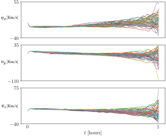
Figure 3: Sample paths for the components $v_{x},v_{y},v_{z}$ of the optimal control for the numerical simulation in Sec. 6.

Fig. 3 shows the corresponding sample paths of the optimal controls.

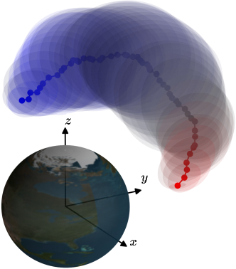
Figure 4: The filled circles show the mean position snapshots for the 50 optimally controlled sample paths in $\mathbb{R}^{3}$, as detailed in Sec. 6. The translucent ellipsoids denote one standard deviation around each mean position.

In Fig. 4, the filled circles depict the evolution (red initial and blue final) of the means of the aforesaid 50 optimally controlled sample path ensemble in $\mathbb{R}^{3}$. The translucent ellipsoids therein display one standard deviations around the means. We include the ECI coordinate in Fig. 4 for reference, and to emphasize that our regularizer in (54) successfully keeps the optimally controlled sample paths above the Earth’s surface.

Fig. 5 plots five snapshots for the univariate $x,y,z$ position marginals computed from the optimally controlled joint PDF $\rho_{\varepsilon}^{\text{opt}}(\bm{r},t)$. This again highlights successful transfer of the stochastic state from given $\rho_{0}$ to given $\rho_{1}$ over the given flight time horizon $[t_{0},t_{1}]$. From Fig. 5, we also note that the optimally controlled marginals (and thus the joint PDFs) at the intermediate times are non-Gaussians even though the endpoints $\rho_{0},\rho_{1}$ are Gaussians in this simulation case study.

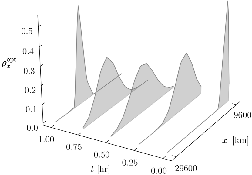
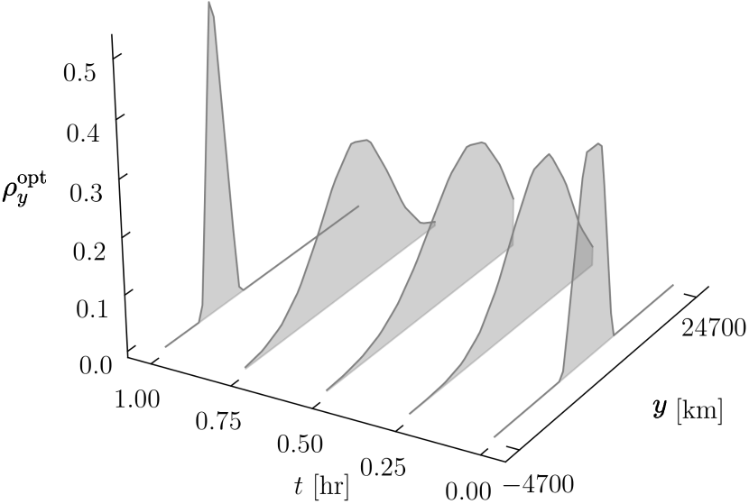
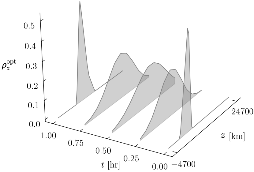
Figure 5: Univariate $x,y,z$ marginals for the optimally controlled joint $\rho_{\varepsilon}^{\text{opt}}(\bm{r},t)$ at $t=0,0.25,0.50,0.75,1$ hours.

7 Conclusion

This work clarifies connections between the probabilistic Lambert problem, the OMT, and the SBP. We showed that the probabilistic Lambert problem is, in fact, a generalized OMT where the gravitational potential plays the role of a state cost. Using Figalli’s theory, we established the existence-uniqueness of solution for this problem. In the presence of stochastic process noise, this problem is shown to become a generalized SBP for which we derived a large deviation principle, thereby proving the existence-uniqueness for this stochastic variant. We derived the associated conditions for optimality, and reduced the same to a boundary-coupled system of reaction-diffusion PDEs where the gravitational potential plays the role of a state-dependent reaction rate. Building on these newfound connections, we presented a novel algorithm and an illustrative numerical case study to demonstrate the solution of the probabilistic Lambert problem via nonparametric computation. Our methods should be of broad interest for solving guidance and navigation problems with stochastic uncertainties at large.

Appendix

7.1 Some Results on Fourier Transform

Let $\iota:=\sqrt{-1}$. We use the non-unitary angular frequency version of Fourier transform

$$\widehat{f}(\bm{\omega}):=\int_{\mathbb{R}^{d}}f(\bm{x})\exp\left(-\iota\langle\bm{\omega},\bm{x}\rangle\right){\rm{d}}\bm{x},$$ (57)

and the corresponding inverse Fourier transform

$$f(\bm{x}):=\dfrac{1}{(2\pi)^{d}}\int_{\mathbb{R}^{d}}\widehat{f}(\bm{\omega})\exp\left(+\iota\langle\bm{\omega},\bm{x}\rangle\right){\rm{d}}\bm{\omega}.$$ (58)

We symbolically write $\widehat{f}(\bm{\omega})=\mathcal{F}\left[f(\bm{x})\right]$, $f(\bm{x})=\mathcal{F}^{-1}\left[\widehat{f}(\bm{\omega})\right]$. We recall the following basic results for a suitably smooth function $f(\bm{x})$ on $\mathbb{R}^{d}$. For brevity, we omit the proofs for these facts.

• (The Fourier transform of Laplacian on $\mathbb{R}^{d}$) $\mathcal{F}\left[\Delta_{\bm{x}}f\right]=-|\bm{\omega}|^{2}\>\widehat{f}(\bm{\omega})$. (59)

• (Convolution) $\mathcal{F}\left[\left(f*g\right)(\bm{x})\right]=\widehat{f}(\bm{\omega})\widehat{g}(\bm{\omega})$, $\mathcal{F}\left[f(\bm{x})g(\bm{x})\right]=\dfrac{1}{(2\pi)^{d}}\left(\widehat{f}*\widehat{g}\right)(\bm{\omega})$. (60)

• (Inverse Fourier transform of exp-neg-square) $\mathcal{F}^{-1}\left[\exp\left(-a|\bm{\omega}|^{2}t\right)\right]=\dfrac{\exp\left(-\frac{|\bm{x}|^{2}}{4at}\right)}{\sqrt{\left(4\pi at\right)^{d}}}$. (61)

7.2 Proof of Lemma 1

We denote the Fourier transform of $u(\bm{x},t)$ w.r.t. $\bm{x}$ as $\widehat{u}(\bm{\omega},t)$ for all $t\in[t_{0},\infty)$, and the Laplace transform of $\widehat{u}(\bm{\omega},t)$ w.r.t. $t$ as $\widehat{U}(\bm{\omega},s)$. Taking the Fourier transform to both sides of (47), we obtain

$$\dfrac{{\rm{d}}}{{\rm{d}}t}\mathcal{F}\left[u(\bm{x},t)\right]=a\mathcal{F}\left[\Delta u\right]+\mathcal{F}\left[b(\bm{x})u\right]\quad\Rightarrow\quad\dfrac{{\rm{d}}}{{\rm{d}}t}\widehat{u}(\bm{\omega},t)=-a|\bm{\omega}|^{2}\>\widehat{u}(\bm{\omega},t)+\dfrac{1}{(2\pi)^{d}}\left(\widehat{b}(\bm{\omega})*\widehat{u}(\bm{\omega},t)\right),$$ (62)

where we used (• ‣ 7.1) and (• ‣ 7.1). Taking the Laplace transform to both sides of (62), we get

$$s\widehat{U}(\bm{\omega},s)-\widehat{u}_{0}(\bm{\omega})=-a|\bm{\omega}|^{2}\>\widehat{U}(\bm{\omega},s)+\dfrac{1}{(2\pi)^{d}}\displaystyle\int_{\mathbb{R}^{d}}\widehat{b}(\bm{\omega}-\bm{\eta})\widehat{U}(\bm{\eta},s)\>{\rm{d}}\bm{\eta}$$

$$\Rightarrow \quad\widehat{U}(\bm{\omega},s)=\dfrac{\widehat{u}_{0}(\bm{\omega})}{s+a|\bm{\omega}|^{2}}+\dfrac{1}{(2\pi)^{d}}\displaystyle\int_{\mathbb{R}^{d}}\widehat{b}(\bm{\omega}-\bm{\eta})\dfrac{\widehat{U}(\bm{\eta},s)}{s+a|\bm{\omega}|^{2}}\>{\rm{d}}\bm{\eta}.$$ (63)

Inverse Laplace transform of (63) yields

$$\widehat{u}(\bm{\omega},t) =\widehat{u}_{0}(\bm{\omega})\exp\left(-a|\bm{\omega}|^{2}t\right)+\dfrac{1}{(2\pi)^{d}}\displaystyle\int_{\mathbb{R}^{d}}\widehat{b}(\bm{\omega}-\bm{\eta})\>\mathcal{L}^{-1}\left[\dfrac{\widehat{U}(\bm{\eta},s)}{s+a|\bm{\omega}|^{2}}\right]\>{\rm{d}}\bm{\eta}$$

$$=\widehat{u}_{0}(\bm{\omega})\exp\left(-a|\bm{\omega}|^{2}t\right)+\dfrac{1}{(2\pi)^{d}}\displaystyle\int_{\mathbb{R}^{d}}\widehat{b}(\bm{\omega}-\bm{\eta})\left(\int_{0}^{t}\widehat{u}(\bm{\eta},\tau)\exp\left(-a|\bm{\omega}|^{2}(t-\tau)\right){\rm{d}}\tau\right){\rm{d}}\bm{\eta},$$

where the last line used the convolution property for the Laplace transform, namely $\mathcal{L}^{-1}\left[F(s)G(s)\right]=\left(f*g\right)(t)$.

We next change the order of integration (using Fubini-Tonelli Theorem) for the space-time integral above, then apply the inverse Fourier transform to both sides, and use (• ‣ 7.1) to arrive at

$$u(\bm{x},t)= \left(u_{0}*\mathcal{F}^{-1}\left[\exp\left(-a|\bm{\omega}|^{2}t\right)\right]\right)(\bm{x})$$

$$+\dfrac{1}{(2\pi)^{d}}\displaystyle\int_{t_{0}}^{t}\left(\mathcal{F}^{-1}\left[\exp\left(-a|\bm{\omega}|^{2}(t-\tau)\right)\right]*\mathcal{F}^{-1}\left[\left(\int_{\mathbb{R}^{d}}\widehat{b}(\bm{\omega}-\bm{\eta})\widehat{u}(\bm{\eta},\tau){\rm{d}}\bm{\eta}\right)\right]\right)(\bm{x})\>{\rm{d}}\tau.$$ (64)

Using (• ‣ 7.1) again, we notice that $\mathcal{F}^{-1}\left[\left(\int_{\mathbb{R}^{d}}\widehat{b}(\bm{\omega}-\bm{\eta})\widehat{u}(\bm{\eta},\tau){\rm{d}}\bm{\eta}\right)\right]=\left(2\pi\right)^{d}b(\bm{x})u(\bm{x},\tau)$, which together with (• ‣ 7.1), simplifies (64) to (48). $\blacksquare$

Funding Sources

This research was supported in part by NSF grant 2112755.

References

• egm [2008 (accessed May 24, 2023] “Earth gravitational model 2008 (EGM2008) data and apps,” https://earth-info.nga.mil/index.php?dir=wgs84&action=wgs84#egm2008, 2008 (accessed May 24, 2023).
• Villani [2003] Villani, C., Topics in optimal transportation, 58, American Mathematical Soc., 2003.
• Villani [2009] Villani, C., Optimal transport: old and new, Vol. 338, Springer, 2009.
• Schrödinger [1931] Schrödinger, E., Über die umkehrung der naturgesetze, Verlag der Akademie der Wissenschaften in Kommission bei Walter De Gruyter u. Company., 1931.
• Schrödinger [1932] Schrödinger, E., “Sur la théorie relativiste de l’électron et l’interprétation de la mécanique quantique,” Annales de l’institut Henri Poincaré, Vol. 2, 1932, pp. 269–310.
• Wakolbinger [1990] Wakolbinger, A., “Schrödinger bridges from 1931 to 1991,” Proc. of the 4th Latin American Congress in Probability and Mathematical Statistics, Mexico City, 1990, pp. 61–79.
• Battin [1977] Battin, R. H., “Lambert’s problem revisited,” AIAA Journal, Vol. 15, No. 5, 1977, pp. 707–713.
• Battin and Vaughan [1984] Battin, R. H., and Vaughan, R. M., “An elegant Lambert algorithm,” Journal of Guidance, Control, and Dynamics, Vol. 7, No. 6, 1984, pp. 662–670.
• Engels and Junkins [1981] Engels, R., and Junkins, J., “The gravity-perturbed Lambert problem: a KS variation of parameters approach,” Celestial mechanics, Vol. 24, No. 1, 1981, pp. 3–21.
• Shen and Tsiotras [2003] Shen, H., and Tsiotras, P., “Optimal two-impulse rendezvous using multiple-revolution Lambert solutions,” Journal of Guidance, Control, and Dynamics, Vol. 26, No. 1, 2003, pp. 50–61.
• McMahon and Scheeres [2016] McMahon, J. W., and Scheeres, D. J., “Linearized Lambert’s problem solution,” Journal of Guidance, Control, and Dynamics, Vol. 39, No. 10, 2016, pp. 2205–2218.
• Junkins and Schaub [2009] Junkins, J. L., and Schaub, H., Analytical mechanics of space systems, American Institute of Aeronautics and Astronautics, 2009.
• Bando and Yamakawa [2010] Bando, M., and Yamakawa, H., “New Lambert algorithm using the Hamilton-Jacobi-Bellman equation,” Journal of Guidance, Control, and Dynamics, Vol. 33, No. 3, 2010, pp. 1000–1008.
• Armellin et al. [2012] Armellin, R., Di Lizia, P., and Lavagna, M., “High-order expansion of the solution of preliminary orbit determination problem,” Celestial Mechanics and Dynamical Astronomy, Vol. 112, 2012, pp. 331–352.
• Schumacher Jr et al. [2015] Schumacher Jr, P. W., Sabol, C., Higginson, C. C., and Alfriend, K. T., “Uncertain Lambert problem,” Journal of Guidance, Control, and Dynamics, Vol. 38, No. 9, 2015, pp. 1573–1584.
• Zhang et al. [2018] Zhang, G., Zhou, D., Mortari, D., and Akella, M. R., “Covariance analysis of Lambert’s problem via Lagrange’s transfer-time formulation,” Aerospace Science and Technology, Vol. 77, 2018, pp. 765–773.
• Adurthi and Majji [2020] Adurthi, N., and Majji, M., “Uncertain Lambert problem: a probabilistic approach,” The Journal of the Astronautical Sciences, Vol. 67, 2020, pp. 361–386.
• Hall and Singla [2018] Hall, Z., and Singla, P., “Higher order polynomial series expansion for uncertain Lambert problem,” AAS Astrodynamics Specialist Conference, 2018.
• Guého et al. [2020] Guého, D., Singla, P., Melton, R. G., and Schwab, D., “A comparison of parametric and non-parametric machine learning approaches for the uncertain Lambert problem,” AIAA Scitech 2020 Forum, 2020, p. 1911.
• Chen et al. [2022] Chen, Y., Georgiou, T. T., and Pavon, M., “The most likely evolution of diffusing and vanishing particles: Schrodinger bridges with unbalanced marginals,” SIAM Journal on Control and Optimization, Vol. 60, No. 4, 2022, pp. 2016–2039.
• Chen et al. [2021] Chen, Y., Georgiou, T. T., and Pavon, M., “Optimal transport in systems and control,” Annual Review of Control, Robotics, and Autonomous Systems, Vol. 4, No. 1, 2021.
• Peyré et al. [2019] Peyré, G., Cuturi, M., et al., “Computational optimal transport: with applications to data science,” Foundations and Trends® in Machine Learning, Vol. 11, No. 5-6, 2019, pp. 355–607.
• Santambrogio [2015] Santambrogio, F., “Optimal transport for applied mathematicians,” Birkäuser, NY, Vol. 55, No. 58-63, 2015, p. 94.
• Tong et al. [2020] Tong, A., Huang, J., Wolf, G., Van Dijk, D., and Krishnaswamy, S., “Trajectorynet: a dynamic optimal transport network for modeling cellular dynamics,” International conference on machine learning, PMLR, 2020, pp. 9526–9536.
• Buttazzo et al. [2012] Buttazzo, G., De Pascale, L., and Gori-Giorgi, P., “Optimal-transport formulation of electronic density-functional theory,” Physical Review A, Vol. 85, No. 6, 2012, p. 062502.
• Ambrosio et al. [2005] Ambrosio, L., Gigli, N., and Savaré, G., Gradient flows: in metric spaces and in the space of probability measures, Springer Science & Business Media, 2005.
• Mei et al. [2018] Mei, S., Montanari, A., and Nguyen, P.-M., “A mean field view of the landscape of two-layer neural networks,” Proceedings of the National Academy of Sciences, Vol. 115, No. 33, 2018, pp. E7665–E7671.
• Halder and Bhattacharya [2014] Halder, A., and Bhattacharya, R., “Probabilistic model validation for uncertain nonlinear systems,” Automatica, Vol. 50, No. 8, 2014, pp. 2038–2050.
• Lee et al. [2015] Lee, K., Halder, A., and Bhattacharya, R., “Performance and robustness analysis of stochastic jump linear systems using Wasserstein metric,” Automatica, Vol. 51, 2015, pp. 341–347.
• Caluya and Halder [2019] Caluya, K. F., and Halder, A., “Gradient flow algorithms for density propagation in stochastic systems,” IEEE Transactions on Automatic Control, Vol. 65, No. 10, 2019, pp. 3991–4004.
• Figalli [2007] Figalli, A., “Optimal transportation and action-minimizing measures,” Ph.D. thesis, Lyon, École normale supérieure (sciences), 2007.
• Dawson et al. [1990] Dawson, D., Gorostiza, L., and Wakolbinger, A., “Schrödinger processes and large deviations,” Journal of mathematical physics, Vol. 31, No. 10, 1990, pp. 2385–2388.
• Aebi and Nagasawa [1992] Aebi, R., and Nagasawa, M., “Large deviations and the propagation of chaos for Schrödinger processes,” Probability Theory and Related Fields, Vol. 94, No. 1, 1992, pp. 53–68.
• Dembo and Zeitouni [2009] Dembo, A., and Zeitouni, O., Large deviations techniques and applications, Vol. 38, Springer Science & Business Media, 2009.
• Benamou and Brenier [2000] Benamou, J.-D., and Brenier, Y., “A computational fluid mechanics solution to the Monge-Kantorovich mass transfer problem,” Numerische Mathematik, Vol. 84, No. 3, 2000, pp. 375–393.
• Halder and Bhattacharya [2011] Halder, A., and Bhattacharya, R., “Dispersion analysis in hypersonic flight during planetary entry using stochastic Liouville equation,” Journal of Guidance, Control, and Dynamics, Vol. 34, No. 2, 2011, pp. 459–474.
• Chen et al. [2015] Chen, Y., Georgiou, T. T., and Pavon, M., “Fast cooling for a system of stochastic oscillators,” Journal of Mathematical Physics, Vol. 56, No. 11, 2015, p. 113302.
• Elamvazhuthi et al. [2018] Elamvazhuthi, K., Grover, P., and Berman, S., “Optimal transport over deterministic discrete-time nonlinear systems using stochastic feedback laws,” IEEE control systems letters, Vol. 3, No. 1, 2018, pp. 168–173.
• Haddad et al. [2020] Haddad, S., Caluya, K. F., Halder, A., and Singh, B., “Prediction and optimal feedback steering of probability density functions for safe automated driving,” IEEE Control Systems Letters, Vol. 5, No. 6, 2020, pp. 2168–2173.
• Caluya and Halder [2021a] Caluya, K. F., and Halder, A., “Wasserstein proximal algorithms for the Schrödinger bridge problem: density control with nonlinear drift,” IEEE Transactions on Automatic Control, Vol. 67, No. 3, 2021a, pp. 1163–1178.
• Caluya and Halder [2021b] Caluya, K. F., and Halder, A., “Reflected Schrödinger bridge: density control with path constraints,” 2021 American Control Conference (ACC), IEEE, 2021b, pp. 1137–1142.
• Nodozi and Halder [2022] Nodozi, I., and Halder, A., “Schrödinger meets Kuramoto via Feynman-Kac: minimum effort distribution steering for noisy nonuniform Kuramoto oscillators,” 2022 IEEE 61st Conference on Decision and Control (CDC), IEEE, 2022, pp. 2953–2960.
• Mikami [2004] Mikami, T., “Monge’s problem with a quadratic cost by the zero-noise limit of h-path processes,” Probability theory and related fields, Vol. 129, No. 2, 2004, pp. 245–260.
• Léonard [2012] Léonard, C., “From the Schrödinger problem to the Monge–Kantorovich problem,” Journal of Functional Analysis, Vol. 262, No. 4, 2012, pp. 1879–1920.
• Léonard [2014] Léonard, C., “A survey of the Schrödinger problem and some of its connections with optimal transport,” Discrete and Continuous Dynamical Systems-Series A, Vol. 34, No. 4, 2014, pp. 1533–1574.
• Kim and Park [2020] Kim, M., and Park, S., “Optimal control approach to Lambert’s problem and Gibbs’ method,” Applied Sciences, Vol. 10, No. 7, 2020, p. 2419.
• Halder and Bhattacharya [2010] Halder, A., and Bhattacharya, R., “Beyond Monte Carlo: a computational framework for uncertainty propagation in planetary entry, descent and landing,” AIAA Guidance, Navigation, and Control Conference, 2010, p. 8029.
• Haddad et al. [2022] Haddad, S., Halder, A., and Singh, B., “Density-based stochastic reachability computation for occupancy prediction in automated driving,” IEEE Transactions on Control Systems Technology, 2022.
• Léonard [2011] Léonard, C., “Stochastic derivatives and generalized h-transforms of Markov processes,” arXiv preprint arXiv:1102.3172, 2011.
• Oksendal [2013] Oksendal, B., Stochastic differential equations: an introduction with applications, Springer Science & Business Media, 2013.
• Karatzas and Shreve [2012] Karatzas, I., and Shreve, S., Brownian motion and stochastic calculus, Vol. 113, Springer Science & Business Media, 2012.
• Csiszár [1984] Csiszár, I., “Sanov property, generalized I-projection and a conditional limit theorem,” The Annals of Probability, 1984, pp. 768–793.
• Hopf [1950] Hopf, E., “The partial differential equation $u_{t}+uu_{x}=\mu_{xx}$,” Communications on Pure and Applied mathematics, Vol. 3, No. 3, 1950, pp. 201–230.
• Cole [1951] Cole, J. D., “On a quasi-linear parabolic equation occurring in aerodynamics,” Quarterly of applied mathematics, Vol. 9, No. 3, 1951, pp. 225–236.
• Hilbert [1895] Hilbert, D., “über die gerade linie als kürzeste verbindung zweier punkte: Aus einem an herrn f. klein gerichteten briefe,” Mathematische Annalen, Vol. 46, No. 1, 1895, pp. 91–96.
• Bushell [1973] Bushell, P. J., “Hilbert’s metric and positive contraction mappings in a Banach space,” Archive for Rational Mechanics and Analysis, Vol. 52, 1973, pp. 330–338.
• Franklin and Lorenz [1989] Franklin, J., and Lorenz, J., “On the scaling of multidimensional matrices,” Linear Algebra and its applications, Vol. 114, 1989, pp. 717–735.
• Chen et al. [2016] Chen, Y., Georgiou, T., and Pavon, M., “Entropic and displacement interpolation: a computational approach using the Hilbert metric,” SIAM Journal on Applied Mathematics, Vol. 76, No. 6, 2016, pp. 2375–2396.
• De Bortoli et al. [2021] De Bortoli, V., Thornton, J., Heng, J., and Doucet, A., “Diffusion Schrödinger bridge with applications to score-based generative modeling,” Advances in Neural Information Processing Systems, Vol. 34, 2021, pp. 17695–17709.
• Pavon et al. [2021] Pavon, M., Trigila, G., and Tabak, E. G., “The data-driven Schrödinger bridge,” Communications on Pure and Applied Mathematics, Vol. 74, No. 7, 2021, pp. 1545–1573.
• Teter et al. [2023] Teter, A. M. H., Chen, Y., and Halder, A., “On the contraction coefficient of the Schrödinger bridge for stochastic linear systems,” IEEE Control Systems Letters, Vol. 7, 2023, pp. 3325–3330. 10.1109/LCSYS.2023.3326836.
• Yong [1997] Yong, J., “Relations among ODEs, PDEs, FSDEs, BSDEs, and FBSDEs,” Proceedings of the 36th IEEE Conference on Decision and Control, Vol. 3, IEEE, 1997, pp. 2779–2784.
• Yong and Zhou [1999] Yong, J., and Zhou, X. Y., Stochastic controls: Hamiltonian systems and HJB equations, Vol. 43, Springer Science & Business Media, 1999.
• Curtis [2013] Curtis, H. D., Orbital mechanics for engineering students, Butterworth-Heinemann, 2013.