Learned Best-Effort LLM Serving

Abstract

Many applications must provide low-latency LLM service to users or risk unacceptable user experience. However, over-provisioning resources to serve fluctuating request patterns is often prohibitively expensive. In this work, we present a best-effort serving system that employs deep reinforcement learning to adjust service quality based on the task distribution and system load. Our best-effort system can maintain availability with over $10\times$ higher client request rates, serves above $96\%$ of peak performance $4.1\times$ more often, and serves above $98\%$ of peak performance $2.3\times$ more often than static serving on unpredictable workloads. Our learned router is robust to shifts in both the arrival and task distribution. Compared to static serving, learned best-effort serving allows for cost-efficient serving through increased hardware utility. Additionally, we argue that learned best-effort LLM serving is applicable in wide variety of settings and provides application developers great flexibility to meet their specific needs.

1 Introduction

Applications in the last decade have evolved from using machine learning in the background for tasks such as data analytics and monitoring to now being at the forefront of user experience. Many applications are using large language models (LLMs) to provide users with both custom and interactive experiences through chat agents and virtual assistants. The need for latency guarantees is critical for such applications as applications cannot simply become unavailable and unresponsive to users. This presents a challenge for LLM serving, as a simple solution of over-provisioning GPU resources to run models in parallel in order to serve bursty request windows is prohibitively expensive for small businesses and independent application developers. Another strategy may be to use a smaller model that serves at lower latency. However, naively using a small model in place of a large model can lead to undesirable quality degradation.

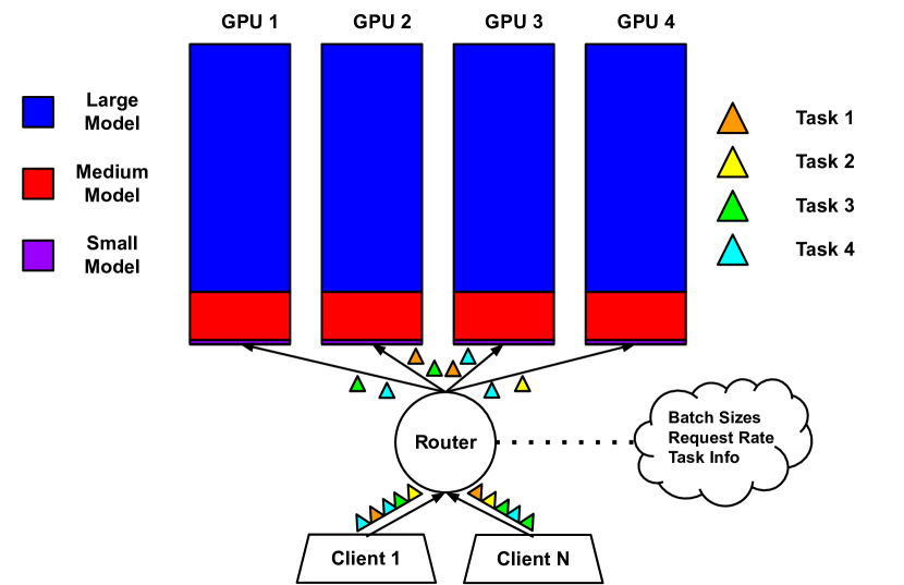
Figure 1: Learned best-effort serving consists of multiple models serving multiple tasks, with a router that keeps track of system load and task information in order to route requests to models. In this example, each model is replicated on 4 GPUs, but any model partitioning and replication scheme may be used. Additionally, any number of models and tasks may be used.

The status-quo for applications is to statically serve queries using a model of fixed quality. For example, within the OPT model family (Zhang et al., 2022), there are models of various sizes, with larger models providing higher quality. An application may choose OPT-6.7B to serve all queries, with this model replicated and/or partitioned across a set of GPUs. However, a model such as OPT-6.7B has much higher latency when compared to smaller models such as OPT-1.3B. To address the challenge of low-latency serving, we explore a new paradigm of best-effort serving in which models of different quality and latency can be selected by the serving system with a router that sends client requests to models as shown in Figure 1. We do not require any changes to the hardware. Serving these smaller models in conjunction with a large model does not inhibit the large model’s serving ability as smaller models consume significantly less device memory than the large model, which has also allowed speculative inference (Leviathan et al., 2023) to become an option for low-latency model serving.

In our problem setup, requests come from a known set of tasks, with larger models providing higher accuracy. Each request has a deadline, which may be either hard or soft, depending on application requirements. Performance for a request is measured as the request’s accuracy if the hard deadline is met. For a soft deadline, the performance decays as the deadline is further violated. It is the goal of the system to maximize the aggregate performance across all requests. Throughout this paper, we refer to “peak performance”, which is further discussed in section 4, as the hypothetical performance achieved by sending all requests to the largest model and always meeting latency deadlines. Our flexible problem formulation allows application developers to best customize how quality and latency are combined into a joint performance metric. We show that routing requests to models is dependent on the set of tasks, the distribution of those tasks, and the load on the system. To navigate this complex relationship, we utilize deep reinforcement learning (RL) techniques with minimal hyper-parameter tuning.

In summary, learned best-effort serving provides a variety of benefits over traditional static serving methods for low-latency LLM applications:

• Increased Performance Learned best-effort serving is able to serve past $96\%$ of peak performance $4.1\times$ more often, and serve past $98\%$ of peak performance $2.3\times$ more often than static serving with a large model on unpredictable and bursty workloads.

• Higher Availability Learned best-effort serving can meet client deadlines at over $10\times$ higher system load than static serving with a large model. Compared to static serving with a medium sized model, learned best-effort serving achieves at least $94\%$ of peak performance $28.21\times$ more often while still providing higher availability.

• Cheaper Serving Learned best-effort serving achieves $3.94\times$ higher performance per hardware unit compared to a static serving baseline that uses double the GPUs. Furthermore the policy still serves past $90\%$ of peak performance $1.51\times$ more often.

2 Preliminaries

2.1 Efficient LLM Serving

The use of multiple models to serve LLM requests has been explored via speculative inference (Leviathan et al., 2023), which uses a small draft model to generate tokens to be verified by a large model. Big Little Decoder is a speculative inference technique (Kim et al., 2023) that allows clients to adjust quality and latency by changing hyper-parameters. However, this requires a hyper-parameter search for every task and does not adjust under load. Furthermore, serving speculative inference in real deployments with optimizations such as continuous batching (Yu et al., 2022) is still an open problem. Dynamically adjusting serving in response to load has been explored though autoscalers. Autoscalers such as Ray (Moritz et al., 2018) dynamically increase GPU instances under load. However, acquiring on-demand GPU instances is expensive and not instantaneous.

2.2 Deep Reinforcement Learning

Deep RL is a promising technique for learning to control systems, and it has been successfully applied in a variety of areas such as continuous controls (Brockman et al., 2016) and games (Mnih et al., 2013). There are three core components in any RL problem: states, actions, and rewards. The RL policy aims to maximize the total rewards it sees as it takes actions and transitions between states. Policy gradient methods aim to differentiate the RL objective directly and perform standard optimization methods to improve the policy. This includes algorithms such as TRPO (Schulman et al., 2015), PPO (Schulman et al., 2017), SAC (Haarnoja et al., 2018), and A3C (Mnih et al., 2016). Deep Q-learning methods learn a Q-function, represented as a neural network, that map state-action pairs to the expected return of taking the action in the state and then following the policy. After fitting the Q-function of the optimal policy, the Q-function may be used to select actions with the highest expected reward. Popular algorithms in this area include DQN (Mnih et al., 2013), Double Q-learning (Van Hasselt et al., 2016), and PER (Schaul et al., 2015).

3 Best-Effort Serving

3.1 Problem Formulation

We consider a scenario of multiple clients who submit requests for LLM inference to an inference system. These requests correspond to specific tasks that are known ahead of time and depend on the application the inference system is providing. Each client request is associated with a specific deadline. The serving system can provide either hard deadlines or soft deadlines. For a hard deadline, performance for a request is measured as the request’s accuracy if the deadline is met. For a soft deadline, the performance decays as the deadline is further violated. It is the goal of the system to maximize the aggregate performance across all requests. In static serving, this is done by sending a request to a predetermined model. In best-effort serving, this is done by dynamically routing requests to different models in order to optimally exploit the latency-quality trade-off.

3.2 Method

As clients submit requests to the inference system, a router routes the request to a specific model. We train this router using a DQN algorithm. Since the policy is a small network, it can be run on the CPU, without needing GPU resources. Quantitatively, running the policy once on our CPU takes only one-tenth of a millisecond. In contrast, on our GPU, generating a token with a small 125M model takes five milliseconds with batch size one and small sequence length. In our RL problem, the state is a vector whose entries denote the task index, the current batch size at each of our models, and an estimate of the arrival rate of client requests. Given this state, the router picks which model to send the client’s request to, which is the action in the RL problem. The reward for picking a specific model in a given state should be a function that increases with higher quality responses but decreases if the client’s deadline is missed. The way in which the reward decreases after missing the deadline is dependent on whether the deadline is a hard deadline or the decay function for a soft deadline. For example, if a hard deadline is missed, the reward of the action should be zero, regardless of the quality.

4 Evaluation

In subsection 4.1, we describe the training procedure, baselines, and evaluated workloads. In subsection 4.2, we describe the models and tasks present in the evaluated serving system. In subsection 4.3 and subsection 4.4, we show that learned best-effort serving outperforms static baselines in both stable and unpredictable workloads, respectively. We show that this holds with both hard and soft deadlines. In subsection 4.5, we show that the learned policy is robust to shifts in the task distribution. In subsection 4.6, we compare learned best-effort serving against a system using twice the GPUs. We show that learned best-effort serving provides both better quality of service as well as significantly higher performance per hardware unit. In subsection 4.7, we demonstrate the policy’s ability to learn and outperform baselines with different deadlines for different requests. Overall, our evaluation highlights multiple advantages provided by learned best-effort serving in a variety of settings.

4.1 Experiment Setup

We train our router’s policy, represented by a 2-layer MLP with hidden size 256, using the DQN algorithm. To prevent over-estimation of Q-values we employ Double Q-learning. We further detail training in Appendix A and use these hyper-parameters for all trained policies. As baselines, we evaluate against static serving with just one model size. When running the baselines, we give all the GPU memory to each model. Graphs with uncertainty regions represent one standard deviation over three trials.

Prior work on model serving (Li et al., 2023; Zhang et al., 2023; Gujarati et al., 2020) uses Microsoft’s Azure Function (MAF) traces (Shahrad et al., 2020; Zhang et al., 2021) to model behavior of clients in a serving system. The MAF1 trace (Shahrad et al., 2020) consists of stable and steady request periods. On the other hand, the MAF2 trace (Zhang et al., 2021) has much more unpredictable client behavior and the arrival rates rapidly change. Based off of these observations, we evaluate our system on three types of synthetic workloads that capture a wide range of client behavior. One workload is stable, while the other two are unpredictable. The synthetic workloads are generated in similar ways to (Yu et al., 2022; Zhang et al., 2023), which use Poisson processes and Markov-modulated Poisson processes. We list further details about the three synthetic workloads and arrival rate estimation in Appendix B.

4.2 System Setup

To evaluate our routing policy, we consider a serving system with 4 GPUs. Each GPU contains an instance of OPT-125M, OPT-1.3B, and OPT-6.7B and there are 4 tasks in the serving system. Thus the serving system is equivalent to the one shown in Figure 1. Smaller models can fit in device memory with the large model because the memory required for both their model parameters, key-value cache, and activations is significantly smaller than those of the large model. Specifically, we give $5\%$ of GPU memory to OPT-125M, $20\%$ of GPU memory to OPT-1.3B, and the rest to OPT-6.7B. When the router chooses a model size for the request, we automatically load balance by sending to the replica with the smallest batch size for the model. We set the latency guarantee to be 40 milliseconds/token. Additionally we use zero-shot HellaSwag (Zellers et al., 2019), COPA (Roemmele et al., 2011), PIQA (Bisk et al., 2020), and OpenBookQA (Mihaylov et al., 2018) as the four tasks in the system. We use each model’s average accuracy on each task as a measure of its quality. For each task we normalize the accuracy of each model to OPT-6.7B’s accuracy to get the rewards shown in Table 1. Our problem formulation is general enough to have the reward function be any increasing function with respect to output quality. An application developer has the flexibility to customize the reward function to best fit their needs. We train the policy for 1.2 million iterations using hard deadlines, a uniform task distribution, and randomly chosen arrival rates with random duration. To prevent out-of-memory issues, we sufficiently limit the maximum batch size of the large model.

Table 1: Rewards for tasks served in the system.

Task	OPT-125M	OPT-1.3B	OPT-6.7B
HellaSwag	0.45	0.78	1.00
COPA	0.80	0.95	1.00
PIQA	0.82	0.96	1.00
OpenBookQA	0.70	0.94	1.00

4.3 Stable Workload

4.3.1 Hard Deadlines

For the stable workload, we vary the arrival rate of the arrival Poisson process from 0.25 to 48 requests per second and serve for 40 seconds at each arrival rate before resetting and going to the next arrival rate. We show the results with hard deadlines in Figure 2. In the hard deadline setting, a client request’s reward is zero if the policy does not pick a model that returns a response to the client within the latency requirements. Therefore we say that the peak performance in this system is one. As baselines, we show the performance when only serving one of OPT-6.7B, OPT-1.3B, or OPT-125M.

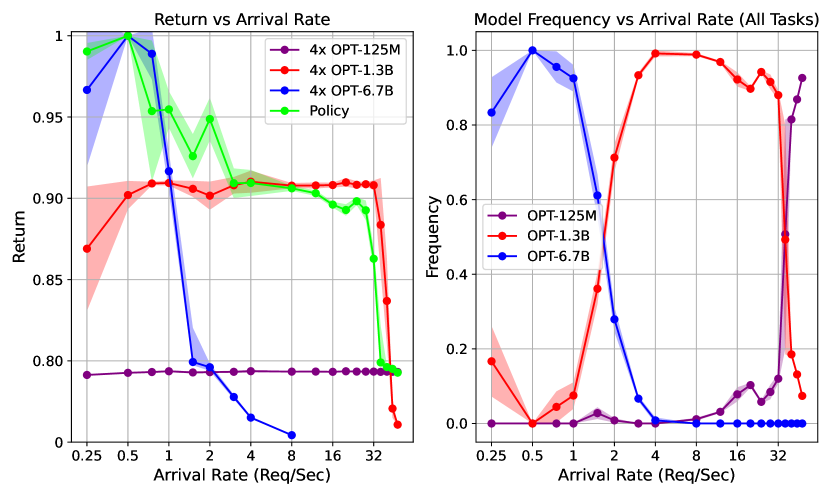
Figure 2: The left figure shows the performance with hard deadlines. The right figure shows the distribution of model selection from the policy.

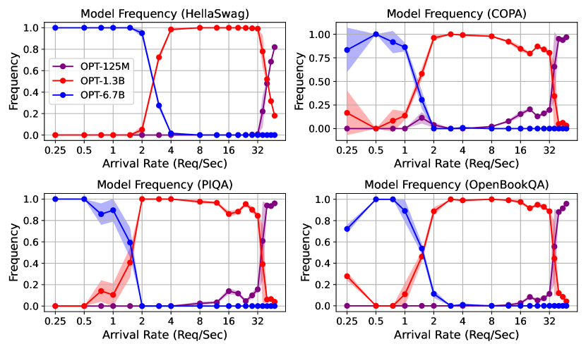
Figure 3: Model selection frequency for each individual task with hard deadlines.

As Figure 2 shows, in typical systems that serve all requests to OPT-6.7B, the performance is near the peak possible performance at low arrival rates. However, once the arrival rate increases past a threshold (2 requests per second), many latency deadlines are missed and performance sharply declines. While OPT-1.3B can serve requests at much higher arrival rates, its quality cannot match OPT-6.7B even when the arrival rate is low. Additionally, there is also a point at which OPT-1.3B cannot keep up with client requests. Serving only with OPT-125M leads to significant performance degradation at all but extremely high arrival rates.

In contrast, the policy dynamically adjusts which model to send requests to. When the arrival rate is low, the policy primarily sends to OPT-6.7B and achieves similar performance. However, as the arrival rate increases, the policy correctly routes more requests to OPT-1.3B and eventually even OPT-125M at the extreme end. Therefore the policy allows the system to remain available for over 10x faster arrival rates than just using OPT-6.7B while still providing equal quality to OPT-6.7B at low arrival rates. Furthermore we notice that there are regions where the policy even performs better than just taking the maximum of each of the baseline’s curves in Figure 2 as it is able to multiplex between models at a given arrival rate.

We now examine how the routing varies for different tasks, as shown in Figure 3. We see that the policy sends HellaSwag requests to OPT-6.7B much more often than the other three tasks. Taking a look at Table 1, we see that OPT-125M and OPT-1.3B have a significant quality gap compared to OPT-6.7B for HellaSwag. This quality gap is much larger than the gap between models on COPA, PIQA, and OpenBookQA. Therefore the policy appropriately learns to prioritize sending HellaSwag to the large model when possible. Furthermore, even when the arrival rate is higher, HellaSwag is sent to OPT-1.3B more often than the other three tasks, which are more frequently sent to OPT-125M. Thus the router learns a complex relationship not only depending on the task’s quality across models in isolation, but with respect to the quality of other tasks in the system and their distribution.

4.3.2 Soft Deadlines

The hard deadline system assumes that a model response is useless to the client at any point after the deadline has passed. While such a strict deadline may be needed for certain applications, many applications are better modeled as a soft deadline system in which performance decays as a non-increasing function of time. It is up to a business and their workload to determine an appropriate soft deadline that matches their system’s requirements.

We pick a specific soft deadline decay function and fine-tune the policy from the policy trained with the hard deadlines. It is also possible to train the soft policy from scratch, but we find that fine-tuning the policy gives good performance. When fine-tuning, we adjust the reward function to be soft and train for an additional 685,000 iterations. Specifically, this soft deadline decays the reward by 1% for every millisecond past the deadline as long as the violation is less than 10% of the specified deadline. However, once the acceptable latency is violated by more than 10%, the client does not value the response and the reward is zero. We show the results in Figure 4. We see that the policy outperforms the baselines and sends more requests to larger models when using this soft deadline than when using hard deadlines. Compared to the hard policy’s performance in Figure 2, we see that the soft policy more closely follows OPT-1.3B’s performance before switching to OPT-125M’s performance. With hard deadlines, the policy takes a slightly more conservative approach in this regime and sends a small set of requests to the small model in order to prevent missing deadlines, creating a small performance gap between the policy and OPT-1.3B before the policy switches to OPT-125M’s performance. With soft deadlines, the policy is less conservative and is able to almost exactly match the performance of OPT-1.3B at these arrival rates.

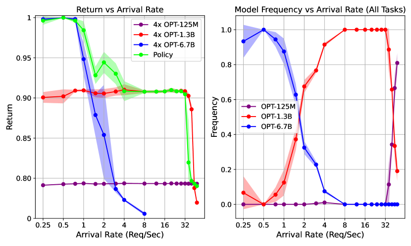
Figure 4: The left figure shows the performance with soft deadlines. The right figure shows the distribution of model selection from the policy.

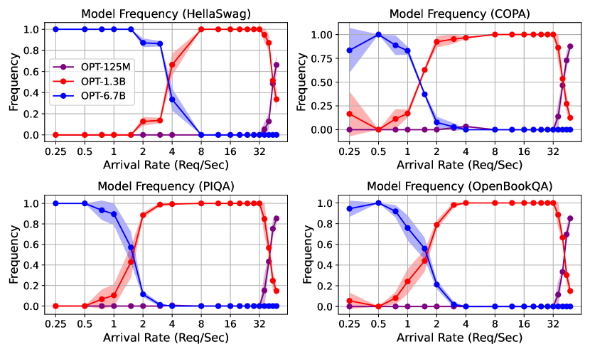
Figure 5: Model selection frequency for each individual task with soft deadlines.

We show how tasks are routed to models when using this soft deadline in Figure 5 and observe similar trends to Figure 3. We approximate the area under the OPT-6.7B selection distribution, using a midpoint Riemann sum, for all tasks in both Figure 5 and Figure 3 to understand the shift in OPT-6.7B selection across tasks. The results, shown in Table 2, show that HellaSwag’s OPT-6.7B usage increases by $52\%$, which is significantly more compared to other tasks when switching from hard deadlines to soft deadlines. The policy is able to exploit the leniency given by the soft deadline to reap the large gains in quality by sending HellaSwag to OPT-6.7B instead of OPT-1.3B.

Table 2: Approximation of OPT-6.7B usage across tasks for both hard and soft deadlines, as measured by Riemann sum of selection distribution.

Task	Hard	Soft	Percent Change
HellaSwag	2.53	3.86	$+52\%$
COPA	1.08	1.16	$+7\%$
PIQA	1.22	1.33	$+9\%$
OpenBookQA	1.30	1.34	$+3\%$

4.4 Unpredictable Workloads

We evaluate on two unpredictable workloads using hard deadlines with large bursts. Both workloads have different arrival patterns than the training workload. Figure 6 shows the performance of the routing policy as well as the baselines, in addition to the changing arrival rate for the first unpredictable workload. We show both the running average of performance across all served requests and the running average of the performance across the last 20 requests. The serving system that only uses OPT-6.7B fails to meet latency deadlines during many of the bursts and thus its performance is highly variable. Even though OPT-6.7B has more windowed averages at peak performance, the policy is able to perform at near-peak performance significantly more often. We quantify this in Table 3.

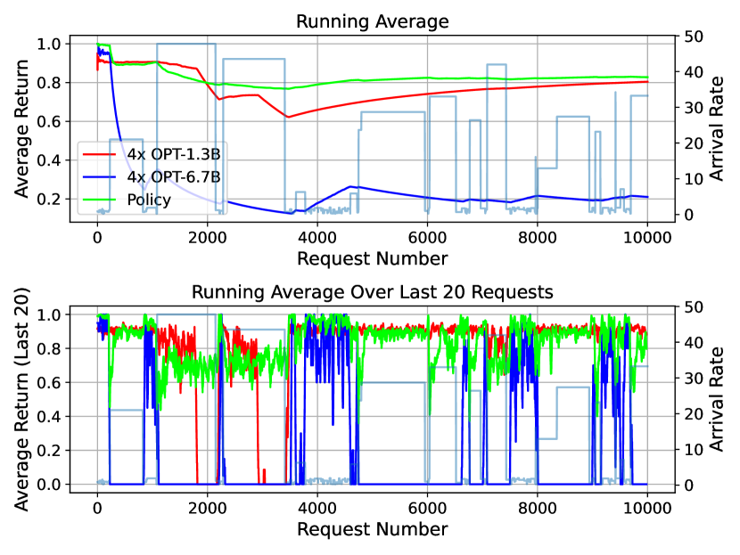
Figure 6: Running total and windowed average over the last 20 requests of performance on the first unpredictable workload. The arrival rate at each step is also shown.

Table 3: Number of request windows of size 20 that meet average performance thresholds on the first unpredictable workload.

Threshold	Policy	OPT-6.7B	OPT-1.3B
$=1.00$	142	307	0
$\geq 0.99$	470	307	0
$\geq 0.98$	713	307	0
$\geq 0.96$	1264	307	0
$\geq 0.94$	1723	625	154

As shown in Table 3, Compared to the policy, OPT-6.7B is able to achieve more windowed averages with peak performance. However, when analyzing the number of windows which meet high performance thresholds such as 0.99, 0.98, 0.96, and 0.94, the policy achieves more such windows than OPT-6.7B and OPT-1.3B. For example, it achieves $1.53\times$ more windows past $99\%$ performance, $2.32\times$ more windows past $98\%$ performance, and $4.11\times$ more windows past $96\%$ performance compared to OPT-6.7B. Additionally, it achieves at least $94\%$ of peak performance $2.75\times$ more often than OPT-6.7B and $11.18\times$ more often than OPT-1.3B. This shows that the policy is able to correctly balance between OPT-6.7B, OPT-1.3B, and OPT-125M, even while faced with an unpredictable workload.

We also show performance on the second unpredictable workload. The results are shown in Figure 7. As the results in Figure 7 show, the policy outperforms both baselines of OPT-1.3B and OPT-6.7B and is able to adapt to the large changes in arrival rate. Additionally, as shown in Table 4, the policy has significantly more windows which meet high performance thresholds. It achieves $1.43\times$ more windows past $99\%$ performance, $2.26\times$ more windows past $98\%$ performance, and $3\times$ more windows past $96\%$ performance compared to OPT-6.7B. Additionally, it achieves at least $94\%$ of peak performance $1.68\times$ more often than OPT-6.7B and $28.21\times$ more often than OPT-1.3B.

Figure 7: Running total and windowed average over the last 20 requests of performance on the second unpredictable workload. The arrival rate at each step is also shown.

Table 4: Number of request windows of size 20 that meet average performance thresholds on the second unpredictable workload.

Threshold	Policy	OPT-6.7B	OPT-1.3B
$=1.00$	447	1378	0
$\geq 0.99$	1977	1378	0
$\geq 0.98$	3121	1378	0
$\geq 0.96$	4141	1378	0
$\geq 0.94$	4740	2810	168

4.5 Robustness to Shifts in Task Distribution

When training the policy we assume that tasks are picked uniformly at random in the application’s workload. For some classes of applications, it is possible that the distribution of tasks changes after the policy has been deployed. It is important that the policy still perform well when the task distribution shifts. We show the performance of our policy in the hard deadline setting while drastically changing the task distribution and without performing any additional training iterations. Specifically, we evaluate performance when the serving system is only receiving requests from one class of tasks at a time. The results on the stable workload are shown in Figure 8. Even though the task distribution is drastically different than the training distribution, the policy is still able to achieve better performance than OPT-6.7B OPT-1.3B, and OPT-125M.

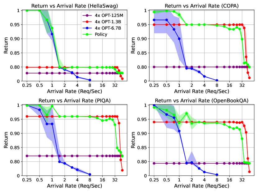
Figure 8: Performance for each of the out-of-distribution workloads, corresponding to sending only one task to the serving system.

We notice that when serving only HellaSwag, the policy closely follows OPT-6.7B’s performance at low arrival rates. In contrast, when only serving COPA, PIQA, or OpenBookQA, the policy is able to outperform OPT-6.7B at these low arrival rates. When analyzing the policy’s model selection distribution for each of the tasks in Figure 9, we see that this is because the policy favors OPT-6.7B on HellaSwag more than the other tasks. Although this was optimal when tasks were picked uniformly at random, it is slightly less optimal now because the policy may benefit from sending some HellaSwag requests to OPT-1.3B due to randomness in the arrival process. For COPA, PIQA, and OpenBookQA, the policy is able to multiplex better with OPT-6.7B and OPT-1.3B and thus is able to beat OPT-6.7B at lower arrival rates. The out-of-distribution performance outperforms the baselines and highlights the policy’s robustness.

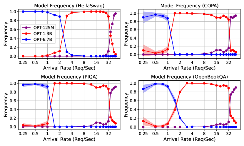
Figure 9: Model selection frequency for each of the out-of-distribution workloads, corresponding to sending only one task to the serving system.

We also evaluate the soft policy’s robustness to distribution shift by sending only HellaSwag and COPA with the arrival patterns of the first unpredictable workload using soft deadlines. We detail the results in Appendix C and show that the soft policy is robust to distribution shift as well.

4.6 Hardware Utility

Our learned router leads to increased performance per hardware unit, which we call hardware utility. To demonstrate this, we compare the performance of running OPT-6.7B replicated on 8 GPUs against running our policy on 4 GPUs. We show the results in Figure 10 on the stable workload using both hard and soft deadlines. When showing the performance, we normalize by the number of GPUs to capture the hardware utility. As Figure 10 shows, the policy running on 4 GPUs significantly outperforms both the 4 and 8 GPU OPT-6.7B system on a per-GPU basis. Additionally, we compare the policy’s hardware utility against the 8 GPU system on the first unpredictable workload and show the results in Figure 11. The policy achieves higher hardware utility than the 8 GPU system $97.03\%$ of the time. On average, the policy’s hardware utility is $3.94\times$ higher than the 8 GPU system. Additionally, the policy serves past $90\%$ of peak performance $1.51\times$ more often than the 8 GPU OPT-6.7B system, when running on just 4 GPUs. Since reserving many GPU instances and having the budget to pay for them are both difficult tasks, these results highlight an important advantage for learned best-effort serving over static serving.

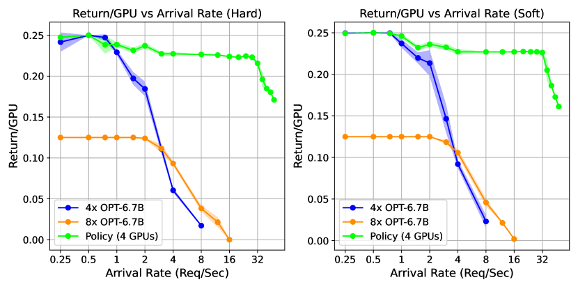
Figure 10: Hardware utility of the policy running on 4 GPUs compared to an OPT-6.7B system running on 8 GPUs. Both hard deadline (left) and soft deadline (right) performance is shown.

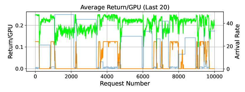
Figure 11: Windowed average over the last 20 requests of the hardware utility of the policy running on 4 GPUs compared to an OPT-6.7B system running on 8 GPUs, on the first unpredictable workload.

4.7 Different Deadlines

Certain applications may want different deadlines to be associated with different tasks. To see if the policy can handle this setting, we double the deadline for OpenBookQA and tighten the deadline for COPA by 20%. We train the policy for 800,000 iterations using hard deadlines and show both the performance and model selection in Figure 12 and Figure 13. We see that the policy is able to learn with different deadlines and outperforms the static serving baselines as before. Additionally, compared to the task-specific selection distribution in Figure 3, the policy sends significantly more OpenBookQA requests to OPT-6.7B, as the deadline is now looser. Compared to the other tasks in the system, the policy waits for a higher arrival rate before it switches sending OpenBookQA requests to OPT-125M instead of OPT-1.3B. Similarly, the policy significantly reduces OPT-6.7B usage for COPA in favor of OPT-1.3B due to the tighter deadlines.

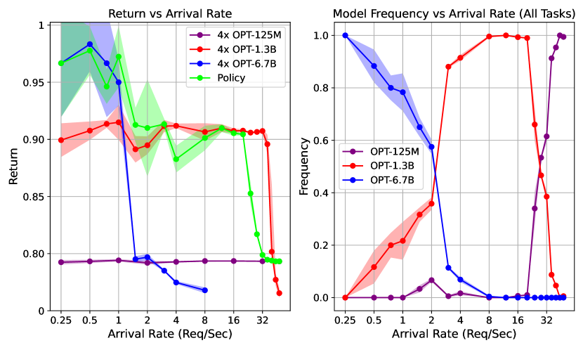
Figure 12: The left figure shows the performance with loose OpenBookQA and tight COPA deadlines. The right figure shows the distribution of model selection from the policy.

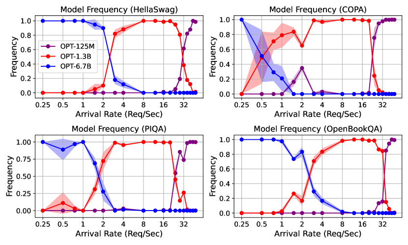
Figure 13: Model selection frequency for each individual task with loose OpenBookQA and tight COPA deadlines.

5 Discussion

Best-effort serving with dynamic routing is an efficient approach for developers looking to scale their latency-sensitive applications. It is also a good option for applications whose client request rates have wide fluctuations, which is common in many practical settings (Zhang et al., 2021). Viewed through another lens, learned best-effort serving allows higher quality during low system load than statically serving a smaller model to handle periods of high loads. There are also a wide range of system environments in which best-effort serving is applicable. Our evaluation in section 4 considered both hard and soft deadlines, as well as different deadlines on different requests. The developed methods are independent of the replication and partitioning strategy of the models. Additionally, our methods can easily be extended to the heterogeneous serving setting. The tasks which we evaluated on all have a notion of accuracy, making it easy to develop a performance function. It is possible that an application requires serving tasks, each of which has a different quality metric such as accuracy, ROUGE (Lin, 2004), BLEU (Papineni et al., 2002), etc. It is up to the application developer’s design to determine how to combine these metrics for their needs. Additionally, application developers may choose to prioritize requests from certain users. For example, many applications offer a paid subscription in exchange for better service. By formulating model serving as a reinforcement learning problem, application developers have the flexibility to adapt the reward function in order to meet their application requirements. For example, they may choose to up-weight the reward on prioritized requests coming from paid users. Lastly, certain applications may want a latency deadline on the first generated token, which can easily be incorporated into the reward function as well.

6 Future Work

In this work we laid the foundation for learned best-effort LLM serving. There are a number of future directions to be explored. When running multiple models on a GPU, there are scheduling decisions on the systems side that need to be made to determine how models share compute resources to further help meet latency deadlines. Additionally, it will be interesting to see extensions to the work that use embeddings or other ways to expand the state in order to capture further information about a client’s request and the state of the system. Lastly, exploring preemption, in which a request’s routing decision is changed as it is being served, may provide benefits on specific workloads.

7 Conclusion

Rather than serving LLMs at a fixed model size, we propose a best-effort serving paradigm with a learned router that maximizes holistic performance, which jointly captures quality latency. We allow latency requirements to be specified as either hard or soft deadlines to represent a wide range of applications. We train our router using deep reinforcement learning methods with minimal hyper-parameter tuning and outperform static serving baselines in a variety of workloads. We show that the router is robust to changes in both the arrival patterns and task distribution. Additionally, learned best-effort serving allows for significantly higher hardware utility compared to static serving. We imagine best-effort serving with dynamic routing to be a cheap and efficient paradigm for latency-sensitive applications.

Appendix A Training Details

We use a discount rate of 0.99, a learning rate of 0.0001, and a batch size of 1024. In our Double Q-learning implementation, the target network is updated every 500 iterations. For exploration, we use an epsilon-greedy strategy. We performed minimal hyper-parameter tuning and use this for all trained policies. All models are served using vLLM (Kwon et al., 2023), which is a state-of-the-art inference serving system. We use an NVIDIA TITAN RTX for GPUs and an Intel Xeon Gold 6126 processor as our CPU.

Appendix B Workload Details

There are three workloads we use - 1 stable and 2 unpredictable. The first represents a stable workload in which client requests arrive in the system as a Poisson process with a fixed rate for a set period of time. The second and third workload represent unpredictable workloads in which the arrival rate of requests rapidly switches due to an underlying stochastic process that controls the arrival rate and its duration. The difference between the second and third workload is that the second workload assumes that the system spends the same amount of time (in expectation) in each arrival rate, while the third workload assumes that the system serves the same amount of requests (in expectation) in each arrival rate before switching. On the unpredictable workloads, we estimate the arrival rate by taking a running average of the last 5 arrivals. It is also possible for application developers to use prior information on the arrival patterns, but we do not use any. Since a near-zero variance estimate of the arrival rate may be obtained on the stable workloads, we give the agent the true arrival rate.

For the first unpredictable workload, we randomly vary the arrival rate and the number of requests served at that arrival rate before switching to the next arrival rate. With 90% probability, we randomly pick an arrival rate between 0.25 and 2. With 8% probability, we randomly pick an arrival rate between 2 and 40. With the remaining 2% probability, we randomly pick an arrival rate between 40 and 48. The number of requests served at the arrival rate is a geometric random variable with mean 20 $\times$ arrival rate.

In the second unpredictable workload, the arrival rate randomly fluctuates between 1 request per second and 48 requests per second. The first unpredictable workload assumed that the expected time spent in each arrival rate is the same. With the new workload, we assume that the number of expected requests seen in each arrival rate is the same, meaning large arrival rates occupy less real time in the system than small arrival rates. We use a geometric random variable with mean 500 to determine the number of requests to serve at an arrival rate before picking the next arrival rate.

Appendix C Additional Task Distribution Shift Experiment

We also evaluate the soft policy’s resistance to shifts in the task distribution on an unpredictable workload. The workload is the first unpredictable workload in subsection 4.4 but requests are chosen uniformly at random between only HellaSwag and COPA. As shown in Figure 14, the policy is still able to outperform the baselines.

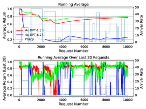
Figure 14: Running total and windowed average over the last 20 requests of performance on the first unpredictable workload while only serving HellaSwag and COPA with soft deadlines. The arrival rate at each step is also shown.

References

- Bisk et al. (2020) Bisk, Y., Zellers, R., Bras, R. L., Gao, J., and Choi, Y. Piqa: Reasoning about physical commonsense in natural language. In Thirty-Fourth AAAI Conference on Artificial Intelligence, 2020.
- Brockman et al. (2016) Brockman, G., Cheung, V., Pettersson, L., Schneider, J., Schulman, J., Tang, J., and Zaremba, W. Openai gym. arXiv preprint arXiv:1606.01540, 2016.
- Gujarati et al. (2020) Gujarati, A., Karimi, R., Alzayat, S., Hao, W., Kaufmann, A., Vigfusson, Y., and Mace, J. Serving DNNs like clockwork: Performance predictability from the bottom up. In 14th USENIX Symposium on Operating Systems Design and Implementation (OSDI 20), pp. 443–462, 2020.
- Haarnoja et al. (2018) Haarnoja, T., Zhou, A., Hartikainen, K., Tucker, G., Ha, S., Tan, J., Kumar, V., Zhu, H., Gupta, A., Abbeel, P., et al. Soft actor-critic algorithms and applications. arXiv preprint arXiv:1812.05905, 2018.
- Kim et al. (2023) Kim, S., Mangalam, K., Malik, J., Mahoney, M. W., Gholami, A., and Keutzer, K. Big little transformer decoder. arXiv preprint arXiv:2302.07863, 2023.
- Kwon et al. (2023) Kwon, W., Li, Z., Zhuang, S., Sheng, Y., Zheng, L., Yu, C. H., Gonzalez, J., Zhang, H., and Stoica, I. Efficient memory management for large language model serving with pagedattention. In Proceedings of the 29th Symposium on Operating Systems Principles, pp. 611–626, 2023.
- Leviathan et al. (2023) Leviathan, Y., Kalman, M., and Matias, Y. Fast inference from transformers via speculative decoding. In International Conference on Machine Learning, pp. 19274–19286. PMLR, 2023.
- Li et al. (2023) Li, Z., Zheng, L., Zhong, Y., Liu, V., Sheng, Y., Jin, X., Huang, Y., Chen, Z., Zhang, H., Gonzalez, J. E., et al. Alpaserve: Statistical multiplexing with model parallelism for deep learning serving. arXiv preprint arXiv:2302.11665, 2023.
- Lin (2004) Lin, C.-Y. Rouge: A package for automatic evaluation of summaries. In Text summarization branches out, pp. 74–81, 2004.
- Mihaylov et al. (2018) Mihaylov, T., Clark, P., Khot, T., and Sabharwal, A. Can a suit of armor conduct electricity? a new dataset for open book question answering. In EMNLP, 2018.
- Mnih et al. (2013) Mnih, V., Kavukcuoglu, K., Silver, D., Graves, A., Antonoglou, I., Wierstra, D., and Riedmiller, M. Playing atari with deep reinforcement learning. arXiv preprint arXiv:1312.5602, 2013.
- Mnih et al. (2016) Mnih, V., Badia, A. P., Mirza, M., Graves, A., Lillicrap, T., Harley, T., Silver, D., and Kavukcuoglu, K. Asynchronous methods for deep reinforcement learning. In International conference on machine learning, pp. 1928–1937. PMLR, 2016.
- Moritz et al. (2018) Moritz, P., Nishihara, R., Wang, S., Tumanov, A., Liaw, R., Liang, E., Elibol, M., Yang, Z., Paul, W., Jordan, M. I., et al. Ray: A distributed framework for emerging AI applications. In 13th USENIX symposium on operating systems design and implementation (OSDI 18), pp. 561–577, 2018.
- Papineni et al. (2002) Papineni, K., Roukos, S., Ward, T., and Zhu, W.-J. Bleu: a method for automatic evaluation of machine translation. In Proceedings of the 40th annual meeting of the Association for Computational Linguistics, pp. 311–318, 2002.
- Roemmele et al. (2011) Roemmele, M., Bejan, C. A., and Gordon, A. S. Choice of plausible alternatives: An evaluation of commonsense causal reasoning. In 2011 AAAI Spring Symposium Series, 2011.
- Schaul et al. (2015) Schaul, T., Quan, J., Antonoglou, I., and Silver, D. Prioritized experience replay. arXiv preprint arXiv:1511.05952, 2015.
- Schulman et al. (2015) Schulman, J., Levine, S., Abbeel, P., Jordan, M., and Moritz, P. Trust region policy optimization. In International conference on machine learning, pp. 1889–1897. PMLR, 2015.
- Schulman et al. (2017) Schulman, J., Wolski, F., Dhariwal, P., Radford, A., and Klimov, O. Proximal policy optimization algorithms. arXiv preprint arXiv:1707.06347, 2017.
- Shahrad et al. (2020) Shahrad, M., Fonseca, R., Goiri, I., Chaudhry, G., Batum, P., Cooke, J., Laureano, E., Tresness, C., Russinovich, M., and Bianchini, R. Serverless in the wild: Characterizing and optimizing the serverless workload at a large cloud provider. In 2020 USENIX annual technical conference (USENIX ATC 20), pp. 205–218, 2020.
- Van Hasselt et al. (2016) Van Hasselt, H., Guez, A., and Silver, D. Deep reinforcement learning with double q-learning. In Proceedings of the AAAI conference on artificial intelligence, volume 30, 2016.
- Yu et al. (2022) Yu, G.-I., Jeong, J. S., Kim, G.-W., Kim, S., and Chun, B.-G. Orca: A distributed serving system for Transformer-Based generative models. In 16th USENIX Symposium on Operating Systems Design and Implementation (OSDI 22), pp. 521–538, 2022.
- Zellers et al. (2019) Zellers, R., Holtzman, A., Bisk, Y., Farhadi, A., and Choi, Y. Hellaswag: Can a machine really finish your sentence? arXiv preprint arXiv:1905.07830, 2019.
- Zhang et al. (2023) Zhang, H., Tang, Y., Khandelwal, A., and Stoica, I. SHEPHERD: Serving DNNs in the wild. In 20th USENIX Symposium on Networked Systems Design and Implementation (NSDI 23), pp. 787–808, 2023.
- Zhang et al. (2022) Zhang, S., Roller, S., Goyal, N., Artetxe, M., Chen, M., Chen, S., Dewan, C., Diab, M., Li, X., Lin, X. V., et al. Opt: Open pre-trained transformer language models. arXiv preprint arXiv:2205.01068, 2022.
- Zhang et al. (2021) Zhang, Y., Goiri, Í., Chaudhry, G. I., Fonseca, R., Elnikety, S., Delimitrou, C., and Bianchini, R. Faster and cheaper serverless computing on harvested resources. In Proceedings of the ACM SIGOPS 28th Symposium on Operating Systems Principles, pp. 724–739, 2021.