Optimal experimental design via gradient flow

Abstract

Optimal experimental design (OED) has far-reaching impacts in many scientific domains. We study OED over a continuous-valued design space, a setting that occurs often in practice. Optimization of a distributional function over an infinite-dimensional probability measure space is conceptually distinct from the discrete OED tasks that are conventionally tackled. We propose techniques based on optimal transport and Wasserstein gradient flow. A practical computational approach is derived from the Monte Carlo simulation, which transforms the infinite-dimensional optimization problem to a finite-dimensional problem over Euclidean space, to which gradient descent can be applied. We discuss first-order criticality and study the convexity properties of the OED objective. We apply our algorithm to the tomography inverse problem, where the solution reveals optimal sensor placements for imaging.

1 Introduction

The problem of inferring unknown parameters from measurements is ubiquitous in real-world engineering contexts, such as biological chemistry [11], medical imaging [22], climate science [16, 51], and infrastructure network design [63, 70, 68]. This problem is termed “parameter identification” [7] and “inverse problems” [59] in the literature. The need to collect informative data economically gives rise to the area of optimal experimental design (OED) [53], which seeks experimental setups that optimize certain statistical criteria.

We denote by $\theta$ the design variable, located in design space $\Omega$. This variable can define boundary location measure or initial data configuration, for instance. Mathematically, the OED problem assigns weights to each possible value of $\theta\in\Omega$ to optimize some statistical criterion. When the design space $\Omega$ is finite, that is, $\Omega=\{\theta_{i}\}_{i=1}^{m}$, the OED weights to be optimized can be gathered in a (finite-dimensional) vector $w=(w_{1},w_{2},\dotsc,w_{m})^{\top}$, with $\sum_{i}w_{i}=1$ and $w\geq 0$. (The latter vector inequality holds component-wise.) In many experiments, however, the design space $\Omega$ has infinite cardinality. One example could be where $\Omega$ contains all possible locations of measurements in a physical domain. For such $\Omega$, the associated weight vector is an infinite-dimensional object; in fact, $w$ becomes a continuous probability measure over $\Omega$. This observation motivates the main question that we address in this paper:

How do we solve the OED problem over a continuous design space?

There is an extensive literature on OED. We summarize relevant works in Section 1.1. The change from finite-dimensional to continuous design space presents many challenges requiring new techniques. To define appropriate metrics for the probability space containing the weight $w$ requires the use of techniques from optimal transport [32] and Wasserstein gradient flow [6]. These methods, though powerful, have yet to be integrated with experimental design. The main contribution of this paper is to make this connection, using gradient flow as our main algorithmic tool. We summarize our contributions and outline the remainder of the paper in Section 1.2.

1.1 Related works

OED has been studied in the literature of statistics, applied mathematics, machine learning, as well as in certain scientific domains. In the earliest stages of OED development, [44] gave rigorous justifications for various design criteria. Computationally, most early OED methods focus on discrete and combinatorial algorithms, manipulating the weights on points in finite design spaces. Notable approaches include sequential algorithms [31, 66, 43, 30], exchange algorithms [10, 67, 48, 46], and multiplicative algorithms [58, 60, 41, 61, 69]. These techniques are related to such optimization methods as constrained gradient descent and nearest-neighbour search.

Progress in scientific computing makes it possible to use OED to handle large-scale simulations for problems from the physical sciences. A prominent example is the Bayesian PDE inverse problem. State-of-the-art results in this area deal with scenarios in which the parametric models are nonlinear [35, 36, 38, 3], infinite-dimensional [2, 3, 1, 4], and ill-posed [34, 4, 54]. They are typically associated with computationally intense forward models. In this regard, new optimization [9] and data-driven methods are exploited to facilitate scalable OED computations, including randomized linear algebra [2, 3, 4, 64], sparse recovery [68, 47, 54, 49, 17, 27] and stochastic optimization [37, 25]. Broader goal-oriented OED frameworks are also investigated in [4, 65].

Another line of research aims to enhance computational efficiency while relaxing the optimality condition. In this regard, sampling and sketching techniques are crucial, especially in works that adopt the perspective of numerical linear algebra. Such methods include fast subset selection [12], importance and volume sampling [28, 29, 50], and random projections [55, 23, 21]. Effectiveness of these techniques follows from concentration inequalities, which produce non-asymptotic accuracy and confidence bounds.

Greedy approaches such as active learning and adaptive sampling have also been applied to OED; see [26, 57, 45, 39, 5] and references therein.

1.2 Our contributions

The main contribution of this paper is a computational framework for solving OED over the continuous design space. Inspired by recent developments in optimal transport, we define a gradient flow scheme for optimizing a smooth probability distribution driven by the OED objective on the Wasserstein metric. We use Monte-Carlo particle approximation to translate the continuum flow of probability measure into gradient-descent flow for the finite set of sample particles, whose evolution captures the dynamics of the underlying infinite-dimensional flow. This evolution can be characterized by a coupled system of ordinary differential equations (ODE). We investigate theoretical aspects of the proposed technique, including convexity, criticality conditions, computation of Fréchet derivatives, and convergence error with respect to key hyperparameters in the particle gradient flow algorithm. Finally, we apply our approach to a problem in medical imaging: electrical impedance tomography (EIT). The experimental design produced by our algorithm provides informative guidance for sensor placement.

The remaining manuscript is organized as follows. We prepare for the technical background on the OED problem and the gradient flow tool in Section 2. In Section 3, we explain gradient flow for optimal design on continuous space, and introduce particle gradient flow algorithm, Algorithm 1. In Section 4, we provide the theoretical properties of continuous OED optimization, including convergence guarantees for Algorithm 1. Finally, we test Algorithm 1 on the EIT inverse problem. Numerical set-up and design performance are explained in Section 5 and Section 6, respectively.

2 Preliminaries and toolkits

We present here the OED problem in its conventional discrete setting (Section 2.1). We then describe Wasserstein gradient flow, a fundamental tool that enables extension of OED to the continuous sampling space (Section 2.2).

2.1 Optimal experimental design

To introduce the classical OED setup, we consider the linear regression model:

$$\mathbf{y}=\mathbf{A}\mathbf{x}^{*}+\boldsymbol{\varepsilon}.$$ (1)

Here, the number of measurements is $m\in\mathbb{N}^{+}$, with observations collected in the vector $\mathbf{y}\in\mathbb{R}^{m}.$ The (linear) forward observation map is denoted by the matrix $\mathbf{A}\in\mathbb{R}^{m\times d}~{}(m\gg d)$, with random noise contributions in the vector $\boldsymbol{\varepsilon}\in\mathbb{R}^{m}$. We wish to infer the parameters $\mathbf{x}^{*}\in\mathbb{R}^{d}.$

For the vastly overdetermined system (1), an estimate of $\mathbf{x}^{*}$ can be obtained without requiring access to the full map $\mathbf{A}$. The aim of OED is to identify a combination of measurements that enables accurate yet economical recovery. Specifically, since each row of the system (1) represents an experiment, we seek a vector $w=(w_{1},w_{2},\dotsc,w_{m})^{\top}$ whose components represent the weights that we assign to each experiment, that solves the following problem:

$$\min_{w}\,F[w]\;\;\mbox{subject to}\;\;w\geq 0,\;\sum_{i=1}^{m}w_{i}=1.$$

The function $F:\mathbb{R}^{m}\to\mathbb{R}$ represents certain design criterion, with smaller objective values of $F$ implying better design.

Many statistical criteria have been proposed for OED. We present the two most commonly used standards [44], denote by the letters “A” (for “average”) and “D” (for “determinant”). They follow from an explanation in terms of Bayesian inference [40, 2].

It is well known that the optimal inference result for (1) that makes use of all data is

$$\hat{\mathbf{x}}=\left(\mathbf{A}^{\top}\mathbf{A}\right)^{-1}\mathbf{A}^{\top}\mathbf{y}.$$

When the noise vector is assumed to follow an i.i.d. Gaussian distribution, that is, $\boldsymbol{\varepsilon}\sim\mathcal{N}(0,\sigma^{2}\mathbf{I}_{m})$, the variance matrix of the solution $\hat{\mathbf{x}}$ is

$$\text{var}(\hat{\mathbf{x}}) = \mathbb{E}\left[(\hat{\mathbf{x}}-\mathbf{x}^{*})(\hat{\mathbf{x}}-\mathbf{x}^{*})^{\top}\right]$$

$$= \mathbb{E}\left[\left(\mathbf{A}^{\top}\mathbf{A}\right)^{-1}\mathbf{A}^{\top}\boldsymbol{\varepsilon}\,\boldsymbol{\varepsilon}^{\top}\mathbf{A}\left(\mathbf{A}^{\top}\mathbf{A}\right)^{-1}\right]$$

$$= \left(\mathbf{A}^{\top}\mathbf{A}\right)^{-1}\mathbf{A}^{\top}\mathbb{E}[\boldsymbol{\varepsilon}\,\boldsymbol{\varepsilon}^{\top}]\mathbf{A}\left(\mathbf{A}^{\top}\mathbf{A}\right)^{-1}$$

$$= \sigma^{2}(\mathbf{A}^{\top}\mathbf{A})^{-1}.$$

The above calculation shows that the inference “uncertainty” depends on the property of the data matrix through the term $(\mathbf{A}^{\top}\mathbf{A})^{-1}$. Smaller variances indicate lower levels of uncertainty and a more accurate reconstruction. We can modify this variance matrix by weighting the experiments using the weights $w$, leading to the following weighted inverse variance [15, Section 7.5]:

$$\mathbf{A}^{\top}\mathbf{A}[w]:=\sum_{k=1}^{m}w_{k}\,\mathbf{A}(k,:)^{\top}\mathbf{A}(k,:).$$ (2)

The OED problem chooses $w$ to minimize a scalar function of the inverse of this weighted variance matrix. The A- and D- design criteria are defined as follows:

$$\text{A-optimal:}\quad\min F^{A}[w] \equiv \text{Tr}\left(\mathbf{A}^{\top}\mathbf{A}[w]\right)^{-1},$$ (3a)

$$\text{D-optimal:}\quad\max F^{D}[w] \equiv \log\left(\text{Det}\left(\mathbf{A}^{\top}\mathbf{A}[w]\right)\right).$$ (3b)

Remark 1.

Note that the design criteria (3a) and (3b) depend solely on the map $\mathbf{A}$, and are independent of the true underlying parameters $\mathbf{x}^{*}$, the measurements $\mathbf{y}$, and the errors $\boldsymbol{\varepsilon}$.

2.2 Wasserstein gradient flow

We describe here the basics of gradient flow [6] and its associated methods. Analogous to gradient descent in Euclidean space, gradient flow optimizes a probability measure objective by defining a flow in the variable space based on a gradient of the objective function. Proper metricization of the space is a critical issue. In this regard, there have been significant advances in optimal transport [56, 32] and Wasserstein gradient flow [42, 6], which we review here.

We require the class of probability measures $\rho$ to have bounded second moments, that is,

$$\mathbf{Pr}_{2}(\Omega)=\left\{\rho~{}~{}\big{|}~{}~{}\rho(\theta)\geq 0~{}~{}\forall\theta\in\Omega,~{}~{}\int_{\Omega}\differential\rho(\theta)=1,~{}~{}\int_{\Omega}|\theta|^{2}\differential\rho(\theta)<\infty\right\}\,.$$ (4)

Note that the probability distribution $\rho$ is not necessarily absolute continuous. Dirac delta functions can be used, enabling practical computations. It is natural to equip the $\mathbf{Pr}_{2}$ space (4) with the Wasserstein-2 metric to measure the distances between probability distributions. For this purpose, we define the joint probability measure $\gamma:\Omega\times\Omega\to\mathbb{R}$ and the set $\Gamma(\mu,\nu)$ to be the space of joint probability measures whose first and second marginals are $\mu,\nu\in\mathbf{Pr}_{2}(\Omega)$, respectively.

Definition 1.

Given the domain $\Omega,$ the Wasserstein-$2$ distance between two probability measures $\mu,\nu\in\mathbf{Pr}_{2}(\Omega)$ is defined as

$$W_{2}(\mu,\nu):=\inf_{\gamma\in\Gamma(\mu,\nu)}\left(\int_{\Omega\times\Omega}\|x-y\|^{2}\differential\gamma(x,y)\right)^{1/2},$$ (5)

where we use the Euclidean $2$-distance in $\Omega$.

For a given objective functional $F:\mathbf{Pr}_{2}(\Omega)\to\mathbb{R}$, we pose the optimization problem

$$\min_{\rho\in\mathbf{Pr}_{2}(\Omega)}F[\rho]\,.$$

From an initial guess for $\rho$, we seek a path in this variable along which $F$ decreases, by making use of the gradient of $F$. The special structure of $\mathbf{Pr}_{2}(\Omega)$ manifold requires care in the definition of the “gradient”. Under the Wassertein-$2$ metric, this gradient is

$$\nabla_{W_{2}}F[\rho]=-\nabla_{\theta}\cdot\left(\rho\,\nabla_{\theta}\frac{\delta F[\rho]}{\delta\rho}\right),$$ (6)

where $\frac{\delta F}{\delta\rho}$ is the Fréchet derivative derived on the $L_{2}$ function space, while the operation $\nabla_{\theta}\cdot\left(\rho\nabla_{\theta}\right)$ defines a “projection” of the $L_{2}$ motion onto the probability measure space. By descending along the negative of this gradient, we obtain the Wasserstein gradient flow of $F$:

$$\partial_{t}\rho=-\nabla_{W_{2}}F[\rho]=\nabla_{\theta}\cdot\left(\rho\,\nabla_{\theta}\frac{\delta F[\rho]}{\delta\rho}\right).$$ (7)

3 Optimal design via gradient flow

In this section, we start by defining the optimal design problem in continuous space, defining continuous analogs of the two objective functions in (3a) and (3b) in the probability measure space, and obtaining expressions for the gradients of these functionals. Next, we define a particle approximation to simulate this gradient flow, as summarized in Algorithm 1, so to optimize the objective functionals.

3.1 Continuous optimal design

In the continuous setting, the “matrix” $\mathbf{A}$ of (1) is no longer finite dimensional. Rather, the rows of $\mathbf{A}$ change continuously over the design space $\Omega$. The sample variable $\theta\in\Omega$ is the row indicator of $\mathbf{A},$ that is, $\mathbf{A}(\theta,:)\in\mathbb{R}^{d}$.

Similar to the weighted matrix product in (2), we define a continuous counterpart:

$$\mathbf{A}^{\top}\mathbf{A}[\rho]=\int_{\Omega}\mathbf{A}(\theta,:)^{\top}\mathbf{A}(\theta,:)\differential\rho(\theta)\in\mathbb{R}.$$ (8)

Accordingly, following the A- and D-optimal discrete design in (3a) and (3b), we arrive at the corresponding criteria in the continuous context:

$$\text{A-optimal:}\quad\rho^{*} := \arg\min_{\rho\in\mathbf{Pr}_{2}(\Omega)}F^{A}[\rho]\equiv\text{Tr}\left(\mathbf{A}^{\top}\mathbf{A}[\rho]\right)^{-1},$$ (9)

$$\text{D-optimal:}\quad\rho^{*} := \arg\max_{\rho\in\mathbf{Pr}_{2}(\Omega)}F^{D}[\rho]\equiv\log\left(\text{Det}\left(\mathbf{A}^{\top}\mathbf{A}[\rho]\right)\right).$$ (10)

To apply Wasserstein gradient flow (7), we need to prepare for the Fréchet derivatives of the OED objectives. We give the explicit calculations below.

Proposition 1.

Assume data matrix $\mathbf{A}$ (1) is full rank. The Fréchet derivatives for (9) and (10) are

$$\frac{\delta F^{A}[\rho]}{\delta\rho}(\theta)=-\mathbf{A}(\theta,:)\left(\mathbf{A}^{\top}\mathbf{A}[\rho]\right)^{-2}\mathbf{A}(\theta,:)^{\top}\,,$$ (11)

and

$$\frac{\delta F^{D}[\rho]}{\delta\rho}(\theta)=\mathbf{A}(\theta,:)\left(\mathbf{A}^{\top}\mathbf{A}[\rho]\right)^{-1}\mathbf{A}(\theta,:)^{\top}\,.$$ (12)

Proof.

Given a probability measure $\rho\in\mathbf{Pr}_{2}(\Omega)$ and a perturbation $\delta\rho:\Omega\to\mathbb{R}$. To get the Fréchet derivative $\frac{\delta F}{\delta\rho}:\Omega\to\mathbb{R}$, we know

$$\int_{\Omega}\frac{\delta F(\theta)}{\delta\rho}\delta\rho(\theta)\differential\theta=\text{the~{}first-order~{}approximation~{}to~{}}F[\rho+\delta\rho]-F[\rho].$$ (13)

For the A-optimal criterion (9), since

$$F^{A}[\rho+\delta\rho]-F^{A}[\rho] = \displaystyle\text{Tr}\left(\mathbf{A}^{\top}\mathbf{A}[\rho+\delta\rho]\right)^{-1}-\text{Tr}\left(\mathbf{A}^{\top}\mathbf{A}[\rho]\right)^{-1}$$

$$= \text{Tr}\left(\left(\mathbf{A}^{\top}\mathbf{A}[\rho]+\mathbf{A}^{\top}\mathbf{A}[\delta\rho]\right)^{-1}-\left(\mathbf{A}^{\top}\mathbf{A}[\rho]\right)^{-1}\right)$$

$$\approx \text{Tr}\left(-\left(\mathbf{A}^{\top}\mathbf{A}[\rho]\right)^{-1}\left(\mathbf{A}^{\top}\mathbf{A}[\delta\rho]\right)\left(\mathbf{A}^{\top}\mathbf{A}[\rho]\right)^{-1}\right).$$

Following more derivations, we obtain

$$\text{Tr}\left(-\left(\mathbf{A}^{\top}\mathbf{A}[\rho]\right)^{-1}\left(\mathbf{A}^{\top}\mathbf{A}[\delta\rho]\right)\left(\mathbf{A}^{\top}\mathbf{A}[\rho]\right)^{-1}\right)$$

$$= \text{Tr}\left(-\left(\mathbf{A}^{\top}\mathbf{A}[\rho]\right)^{-2}\mathbf{A}^{\top}\mathbf{A}[\delta\rho]\right)$$

$$= \text{Tr}\left(-\left(\mathbf{A}^{\top}\mathbf{A}[\rho]\right)^{-2}\int_{\Omega}\mathbf{A}(\theta,:)^{\top}\mathbf{A}(\theta,:)\delta\rho(\theta)\differential\theta\right)$$

$$= \int_{\Omega}\text{Tr}\left(-\left(\mathbf{A}^{\top}\mathbf{A}[\rho]\right)^{-2}\mathbf{A}(\theta,:)^{\top}\mathbf{A}(\theta,:)\right)\,\delta\rho(\theta)\differential\theta$$

$$= \int_{\Omega}-\mathbf{A}(\theta,:)\left(\mathbf{A}^{\top}\mathbf{A}[\rho]\right)^{-2}\mathbf{A}(\theta,:)^{\top}\,\delta\rho(\theta)\differential\theta$$

$$= \int_{\Omega}\frac{\delta F^{A}(\theta)}{\delta\rho}\delta\rho(\theta)\differential\theta.$$

The above results utilize the fact that the trace of matrix products is commutative (lines 2 and 5) and also trace, integration operations are interchangeable (line 4).

From the last two equations above, we obtain the derivative of A-design:

$$\frac{\delta F^{A}(\theta)}{\delta\rho}=-\mathbf{A}(\theta,:)\left(\mathbf{A}^{\top}\mathbf{A}[\rho]\right)^{-2}\mathbf{A}(\theta,:)^{\top}.$$

A similar derivations holds for the D-optimal objective (10). We consider

$$F^{D}[\rho+\delta\rho]-F^{D}[\rho]=\log\left(\text{Det}\left(\mathbf{A}^{\top}\mathbf{A}[\rho+\delta\rho]\right)\right)-\log\left(\text{Det}\left(\mathbf{A}^{\top}\mathbf{A}[\rho]\right)\right).$$

The linear approximation to the first term on RHS is

$$\log\left(\text{Det}\left(\mathbf{A}^{\top}\mathbf{A}[\rho+\delta\rho]\right)\right)$$

$$\approx \log\left(\text{Det}\left(\mathbf{A}^{\top}\mathbf{A}[\rho]\right)+\text{Det}\left(\mathbf{A}^{\top}\mathbf{A}[\rho]\right)\,\text{Tr}\left((\mathbf{A}^{\top}\mathbf{A}[\rho])^{-1}\mathbf{A}^{\top}\mathbf{A}[\delta\rho]\right)\right)$$

$$= \log\left(\text{Det}\left(\mathbf{A}^{\top}\mathbf{A}[\rho]\right)\right)+\frac{1}{\text{Det}\left(\mathbf{A}^{\top}\mathbf{A}[\rho]\right)}\text{Det}\left(\mathbf{A}^{\top}\mathbf{A}[\rho]\right)\,\text{Tr}\left((\mathbf{A}^{\top}\mathbf{A}[\rho])^{-1}\mathbf{A}^{\top}\mathbf{A}[\delta\rho]\right)$$

$$= \log\left(\text{Det}\left(\mathbf{A}^{\top}\mathbf{A}[\rho]\right)\right)+\text{Tr}\left((\mathbf{A}^{\top}\mathbf{A}[\rho])^{-1}\mathbf{A}^{\top}\mathbf{A}[\delta\rho]\right).$$

(The second line is due to the Jacobi’s formula for derivative of matrix determinant, while the third line is by applying the derivative of log function.) We then have the linear difference term for $F^{D}$:

$$F^{D}[\rho+\delta\rho]-F^{D}[\rho] \approx \text{Tr}\left((\mathbf{A}^{\top}\mathbf{A}[\rho])^{-1}\mathbf{A}^{\top}\mathbf{A}[\delta\rho]\right)$$

$$= \int_{\Omega}\mathbf{A}(\theta,:)^{\top}(\mathbf{A}^{\top}\mathbf{A}[\rho])^{-1}\mathbf{A}(\theta,:)\,\delta\rho(\theta)\differential\theta$$

$$= \int_{\Omega}\frac{\delta F^{D}(\theta)}{\delta\rho}\delta\rho(\theta)\differential\theta.$$

(The second step above is similar to the penultimate equality in (3.1).) We finally obtain the D design derivative:

$$\frac{\delta F^{D}(\theta)}{\delta\rho}=\mathbf{A}(\theta,:)\left(\mathbf{A}^{\top}\mathbf{A}[\rho]\right)^{-1}\mathbf{A}(\theta,:)^{\top}.$$

∎

3.2 Particle gradient flow

Proposition 1 in combination with (7) defines the gradient flow for finding the OED probability measure over the design space $\Omega$. Classical techniques for solving this PDE formulation involve discretizing $\Omega$ and tracing the evolution of $\rho$ on the mesh. This strategy presents a computational challenge: The size of the mesh (or equivalently, the degrees of freedom required to represent $\rho$ in the discrete setting) grows exponentially with the dimension of the design space. The computational complexity required to implement this strategy would exceed the experiment budget, in terms of the optimized weighting object size and total measurements.

One advantage of employing the Wasserstein gradient flow is its close relationship to a particle ODE interpretation [20, 13, 24]. We can use Monte Carlo to represent the probability measure $\rho$ by a particle samples on the design space $\Omega$. This simulation translates the PDE into a coupled ODE system on the sample vector $\theta\in\Omega$. Following the descending trajectory of (7), when $\rho$ is known, the characteristic of this PDE is

$$\frac{\differential\theta}{\differential t}=-\nabla_{\theta}\frac{\delta F[\rho]}{\delta\rho}(\theta).$$ (15)

In computation, the distribution $\rho$ is unknown, but we can use an empirical measure for the approximation to $\rho$. Given a fixed number of particles $N\in\mathbb{N}^{+},$ we consider a set of particles $\{\theta_{i}\}_{i=1}^{N}\subset\Omega.$ The estimated probability $\rho$ is the average of Dirac-delta measures at selected particles $\rho_{N}$, that is,

$$\rho\approx\rho_{N}=\frac{1}{N}\sum_{i=1}^{N}\delta_{\theta_{i}}\in\mathbf{Pr}_{2}(\Omega).$$ (16)

The discrete approximation $\rho_{N}$ is better able to approximate the continuous range of $\Omega$ than a costly setup where the discretization is predefined in Section 3.2. By inserting the empirical measure (16) into (15), and employing forward-Euler time integration, we arrive at the following particle gradient flow algorithm method.

Algorithm 1 Particle gradient flow

Input: Number of particles $N$; number of iterations $T$; time step $\differential t$
initial particles $\theta_{1}^{0},\dotsc,\theta_{N}^{0}\subset\Omega$ and starting measure $\rho^{0}_{N}=\frac{1}{N}\sum_{i=1}^{N}\delta_{\theta^{0}_{i}}$
Output: probability measure $\rho\in\mathbf{Pr}_{2}(\Omega)$

1:for $t=1,\dotsc,T$ do

2:     for $i=1,\dotsc,N$ do

3:         $\displaystyle\theta^{t}_{i}\leftarrow\theta^{t-1}_{i}-\differential t\,\nabla_{\theta}\frac{\delta F[\rho_{N}^{t-1}]}{\delta\rho}(\theta_{i}^{t-1})$ $\triangleright$ update particles (descent)

4:     end for

5:     $\displaystyle\rho_{N}^{t}\leftarrow\sum_{i=1}^{N}\frac{1}{N}\delta_{\theta_{i}^{t}}$ $\triangleright$ update probability measure

6:end for

7:return $\rho\leftarrow\rho_{N}^{T}$

Remark 2.

Line 3 of Algorithm 1 is the descent update formula for minimization of $F$. For maximization, as in the D-optimal design (10), we switch the minus sign to plus to obtain ascent.

Algorithm 1 requires calculation of the particle velocity forms $\nabla_{\theta}\frac{\delta F[\rho_{N}]}{\delta\rho}$ for A- and D-optimal design criteria (9), (10). Details of this computation are shown in the next result.

Proposition 2.

Fix a set of particles $\{\theta_{i}\}_{i=1}^{N}\subset\Omega$ and consider the empirical measure (16). The flow field of a sample particle $\theta\in\Omega$ under the A-optimal objective (9) is

$$\nabla_{\theta}\frac{\delta F^{A}[\rho_{N}]}{\delta\rho}(\theta)=-2\,\nabla_{\theta}\mathbf{A}(\theta,:)\left(\frac{1}{N}\sum_{i=1}^{N}\mathbf{A}(\theta_{i},:)^{\top}\mathbf{A}(\theta_{i},:)\right)^{-2}\mathbf{A}(\theta,:)^{\top}.$$ (17)

For the D-optimal objective (10) the flow field is

$$\nabla_{\theta}\frac{\delta F^{D}[\rho_{N}]}{\delta\rho}(\theta)=2\,\nabla_{\theta}\mathbf{A}(\theta,:)\left(\frac{1}{N}\sum_{i=1}^{N}\mathbf{A}(\theta_{i},:)^{\top}\mathbf{A}(\theta_{i},:)\right)^{-1}\mathbf{A}(\theta,:)^{\top}.$$ (18)

Proof.

For the empirical measure (16), the sampled target (8) is

$$\mathbf{A}^{\top}\mathbf{A}[\rho_{N}]=\frac{1}{N}\sum_{i=1}^{N}\mathbf{A}(\theta_{i},:)^{\top}\mathbf{A}(\theta_{i},:).$$

We plug the above term respectively in the Fréchet derivatives of (11) and(12). For any particle $\theta\in\Omega,$ we obtain

$$\frac{\delta F^{A}[\rho_{N}]}{\delta\rho}(\theta) = -\mathbf{A}(\theta,:)\left(\frac{1}{N}\sum_{i=1}^{N}\mathbf{A}(\theta_{i},:)^{\top}\mathbf{A}(\theta_{i},:)\right)^{-2}\mathbf{A}(\theta,:)^{\top},$$

$$\frac{\delta F^{D}[\rho_{N}]}{\delta\rho}(\theta) = \mathbf{A}(\theta,:)\left(\frac{1}{N}\sum_{i=1}^{N}\mathbf{A}(\theta_{i},:)^{\top}\mathbf{A}(\theta_{i},:)\right)^{-1}\mathbf{A}(\theta,:)^{\top}.$$

Note that in the computation for both derivatives, the middle matrix terms are already evaluated at fixed values $\{\theta_{i}\}_{i=1}^{N}$ and thus are independent of $\theta$. When taking the gradient with respect to $\theta$, only the first and the third terms contribute, and we arrive at

$$\nabla_{\theta}\frac{\delta F^{A}[\rho_{N}]}{\delta\rho}(\theta) = -2\,\nabla_{\theta}\mathbf{A}(\theta,:)\left(\frac{1}{N}\sum_{i=1}^{N}\mathbf{A}(\theta_{i},:)^{\top}\mathbf{A}(\theta_{i},:)\right)^{-2}\mathbf{A}(\theta,:)^{\top},$$

as required. The gradient for the D-optimal objective follows similarly:

$$\nabla_{\theta}\frac{\delta F^{D}[\rho_{N}]}{\delta\rho}(\theta)=2\,\nabla_{\theta}\mathbf{A}(\theta,:)\left(\frac{1}{N}\sum_{i=1}^{N}\mathbf{A}(\theta_{i},:)^{\top}\mathbf{A}(\theta_{i},:)\right)^{-1}\mathbf{A}(\theta,:)^{\top}.$$

∎

4 Theoretical guarantees

We provide some theoretical properties regarding the continuous OED and the proposed Algorithm 1. We study the first-order critical condition and the convexity of the OED objective functionals in Section 4.1 and Section 4.2 respectively. In Section 4.3, we discuss the convergence of Algorithm 1.

4.1 First-order critical condition

We first lay out the stationary point condition under the $W_{2}$ metric.

Lemma 1.

The distribution $\rho^{\ast}\in\mathbf{Pr}_{2}(\Omega)$ is a stationary solution to $\min_{\rho\in\mathbf{Pr}_{2}(\Omega)}$ or $\max_{\rho\in\mathbf{Pr}_{2}(\Omega)}F[\rho]$ — that is, $\partial_{t}\rho^{\ast}=0$ — if it satisfies the first-order critical condition:

$$\nabla_{\theta}\frac{\delta F[\rho^{*}]}{\delta\rho}(\theta)=0,\quad\forall~{}\theta\in\text{\rm supp}(\rho^{*}).$$ (19)

Proof.

We present the proof for the minimization problem. (The proof for maximization is similar.)

In the Wasserstein flow of $\rho\in\mathbf{Pr}_{2}(\Omega)$, the differential of the objective $F$ is

$$\frac{\differential F[\rho]}{\differential t}=\int_{\Omega}\frac{\delta F[\rho]}{\delta\rho}(\theta)\,\partial_{t}\rho(\theta)\,\differential\theta.$$ (20)

When we substitute for $\partial_{t}\rho$ from (7), we obtain

$$\frac{\differential F[\rho]}{\differential t}=\int_{\Omega}\frac{\delta F[\rho]}{\delta\rho}(\theta)\,\nabla_{\theta}\,\cdot\left(\rho\nabla_{\theta}\frac{\delta F[\rho]}{\delta\rho}\right)\differential\theta=-\int_{\Omega}\rho(\theta)\left|\nabla_{\theta}\frac{\delta F[\rho]}{\delta\rho}\right|^{2}\,\differential\theta\leq 0.$$ (21)

The last derivation is from the Green’s identity and the assumption that the velocity term $\nabla_{\theta}\frac{\delta F[\rho]}{\delta\rho}$ vanishes on the boundary $\partial\Omega.$

First-order criticality conditions for $\rho^{*}$ are $\frac{\differential F[\rho^{*}]}{\differential t}=0$. Hence equation (21) implies that the critical condition (19) is required for the integrand in (21) to be zero everywhere in $\Omega.$ ∎

Therefore in the $W_{2}$ descent flow (7), the objective $F$ keeps decreasing until $\rho$ achieves stationarity. (A similar claim applies to ascent in the maximization case.) The critical condition (19) does not give the explicit stationary measure $\rho^{*}$ except in special cases, one of which we present now.

Proposition 3.

Suppose the data matrix $\mathbf{A}$ of model problem (1) contains a subset of orthogonal rows $\{\mathbf{A}(\theta_{i},:)\}_{i=1}^{d}$ with row indices $\{\theta_{i}\}_{i=1}^{d}\subset\Omega$, and satisfies

$$\nabla_{\theta}\mathbf{A}(\theta_{i},:)\perp\mathbf{A}(\theta_{i},:)\,,\quad\forall i\in[d].$$ (22)

Then the following form satisfies the A- (9) and D-optimal (10) design criteria:

$$\rho^{*}=\sum_{i=1}^{d}\alpha_{i}\delta_{\theta_{i}},\quad\text{s.t.}~{}\sum_{i=1}^{d}\alpha_{i}=1,~{}~{}\alpha_{i}>0,~{}\forall i\in[d].$$ (23)

Proof.

By rescaling the orthogonal rows $\mathbf{A}(\theta_{i},:)$ for $i\in[d]$ we can define an orthogonal matrix $\mathbf{U}\in\mathbb{R}^{d\times d}$ with rows $\mathbf{U}(i,:)$ defined by

$$\mathbf{U}(i,:)=\frac{\mathbf{A}(\theta_{i},:)}{\|\mathbf{A}(\theta_{i},:)\|},\quad\forall i\in[d].$$ (24)

For the sampled target by $\rho^{*}$, we obtain from this formula and (2) that

$$\mathbf{A}^{\top}\mathbf{A}[\rho^{*}]=\sum_{i=1}^{d}\alpha_{i}\mathbf{A}(\theta_{i},:)^{\top}\mathbf{A}(\theta_{i},:)=\mathbf{U}^{\top}\mathbf{C}\mathbf{U},$$

where $\mathbf{C}\in\mathbb{R}^{d\times d}$ is a diagonal matrix with $i$th diagonal $\mathbf{C}(i,i)=\alpha_{i}\|\mathbf{A}(\theta_{i},:)\|^{2}$. We thus have by orthogonality of $\mathbf{U}$ that

$$\left(\mathbf{A}^{\top}\mathbf{A}[\rho^{*}]\right)^{-1}=\mathbf{U}^{\top}\mathbf{C}^{-1}\mathbf{U},\quad\left(\mathbf{A}^{\top}\mathbf{A}[\rho^{*}]\right)^{-2}=\mathbf{U}^{\top}\mathbf{C}^{-2}\mathbf{U}.$$

For $\theta_{i}\in\text{supp}(\rho^{*}),$ the A-optimal derivative is

$$\displaystyle\nabla_{\theta}\frac{\delta F^{A}[\rho^{*}]}{\delta\rho}(\theta_{i}) = \displaystyle\nabla_{\theta}\mathbf{A}(\theta_{i},:)\left(\mathbf{A}^{\top}\mathbf{A}[\rho^{*}]\right)^{-2}\mathbf{A}(\theta_{i},:)^{\top}$$

$$= \displaystyle\nabla_{\theta}\mathbf{A}(\theta_{i},:)\mathbf{U}^{\top}\mathbf{C}^{-2}\mathbf{U}\mathbf{A}(\theta_{i},:)^{\top}.$$ (25)

Since $\{\mathbf{A}(\theta_{i},:)\}_{i=1}^{d}$ have orthogonal rows, we have from (24) that

$$\mathbf{C}^{-2}\mathbf{U}\mathbf{A}(\theta_{i},:)^{\top}=\|\mathbf{A}(\theta_{i},:)\|\mathbf{C}^{-2}\mathbf{U}\mathbf{U}(i,:)^{\top}=\frac{\|\mathbf{A}(\theta_{i},:)\|}{\mathbf{C}(i,i)^{2}}\mathbf{e}_{i}.$$

By substituting into (25) and using (24) again, we obtain

$$\displaystyle\nabla_{\theta}\frac{\delta F^{A}[\rho^{*}]}{\delta\rho}(\theta_{i}) = \displaystyle\nabla_{\theta}\mathbf{A}(\theta_{i},:)\mathbf{U}^{\top}\mathbf{e}_{i}\frac{\|\mathbf{A}(\theta_{i},:)\|}{\mathbf{C}(i,i)^{2}}$$

$$= \displaystyle\nabla_{\theta}\mathbf{A}(\theta_{i},:)\mathbf{U}(i,:)^{\top}\frac{\|\mathbf{A}(\theta_{i},:)\|}{\mathbf{C}(i,i)^{2}}$$

$$= \displaystyle\nabla_{\theta}\mathbf{A}(\theta_{i},:)\mathbf{A}(\theta_{i},:)^{\top}\frac{1}{\mathbf{C}(i,i)^{2}}$$

$$= 0,$$

where the final equality is a consequence of (22).

A similar argument shows that $\nabla_{\theta}\frac{\delta F^{D}[\rho^{*}]}{\delta\rho}(\theta_{i})=0$.

Since the gradient of the Fréchet derivative is $0$ for all support points $\theta_{i}$, $\rho^{*}$ satisfies the first-order criticality condition (19). ∎

4.2 Convexity of design objectives

Another feature of the OED problems (9)-(10) is that they are convex optimization problems in the $L_{2}$ sense, as we explain next.

Proposition 4.

For any probability measure $\rho\in\mathbf{Pr}_{2}(\Omega)$ that ensures invertibility of the matrix $\mathbf{A}^{\top}\mathbf{A}[\rho]$ defined in (8), the objective functionals for both A-optimal and D-optimal defined in (9) and (10) are second order differentiable. Moreover, the Hessian functionals $\text{Hess}~{}F^{A}[\rho]$ and $\text{Hess}~{}F^{D}[\rho]$ are positive and negative semidefinite operators respectively, so both problems are convex optimization problems in the $L_{2}$ sense.

Proof.

Fix a probability distribution $\rho\in\mathbf{Pr}_{2}(\Omega),$ we will explicitly compute the two Hessian terms. For any given two perturbation measures $\delta\rho_{1},\delta\rho_{2}:\Omega\to\mathbb{R}$. The bilinear Hessian operator is computed by:

$$\text{Hess}~{}F[\rho](\delta\rho_{1},\delta\rho_{2})$$

$$= \lim_{\epsilon\to 0}\frac{(F[\rho+\varepsilon\delta\rho_{1}+\varepsilon\delta\rho_{2}]-F[\rho+\varepsilon\delta\rho_{2}])-(F[\rho+\varepsilon\delta\rho_{1}]-F[\rho])}{\varepsilon^{2}}$$

$$\approx \lim_{\varepsilon\to 0}\frac{1}{\varepsilon}\left(\int_{\Omega}\frac{\delta F[\rho+\varepsilon\delta\rho_{2}]}{\delta\rho}\delta\rho_{1}(\theta)\,\differential\theta-\int_{\Omega}\frac{\delta F[\rho]}{\delta\rho}\delta\rho_{1}(\theta)\,\differential\theta\right)\,.$$

The last derivation is from the definition of Fréchet derivative (13).

For positive definiteness, we need $\text{Hess}~{}F[\rho](\delta\rho,\delta\rho)\geq 0$ for all $\delta\rho$. Since the sign is kept in the process of passing the limit, we will study the first-order expansion of

$$\int_{\Omega}\frac{\delta F[\rho+\varepsilon\delta\rho]}{\delta\rho}\delta\rho(\theta)\,\differential\theta-\int_{\Omega}\frac{\delta F[\rho]}{\delta\rho}\delta\rho(\theta)\,\differential\theta\geq 0,\quad\forall~{}\varepsilon\in\mathbb{R}.$$ (27)

Regarding (8), we define the following shorthand notation:

$$\mathbf{M}:=\mathbf{A}^{\top}\mathbf{A}[\rho]\in\mathbb{R}^{d\times d},\quad\mathbf{D}:=\mathbf{A}^{\top}\mathbf{A}[\delta\rho]\in\mathbb{R}^{d\times d}.$$ (28)

(Note that the theorem assumes positive definiteness of $\mathbf{M}$.)

We first study the A-optimal design objective (9). For the first term in (27), we deploy (11) from Proposition 1 to obtain

$$\int_{\Omega}\frac{\delta F^{A}[\rho+\varepsilon\delta\rho]}{\delta\rho}\delta\rho(\theta)\,\differential\theta=-\displaystyle\int_{\Omega}\mathbf{A}(\theta,:)\left(\mathbf{A}^{\top}\mathbf{A}[\rho+\varepsilon\delta\rho]\right)^{-2}\mathbf{A}(\theta,:)^{\top}\delta\rho(\theta)\differential\theta.$$

Since the integrand is a scalar, it is equivalent to its trace value. Thus the expression above is equal to

$$\begin{array}[]{l}-\displaystyle\int_{\Omega}\text{Tr}\left(\mathbf{A}(\theta,:)\left(\mathbf{A}^{\top}\mathbf{A}[\rho+\varepsilon\delta\rho]\right)^{-2}\mathbf{A}(\theta,:)^{\top}\right)\delta\rho(\theta)\differential\theta\\ =\displaystyle-\int_{\Omega}\text{Tr}\left(\left(\mathbf{A}^{\top}\mathbf{A}[\rho+\varepsilon\delta\rho]\right)^{-2}\mathbf{A}(\theta,:)^{\top}\mathbf{A}(\theta,:)\right)\delta\rho(\theta)\differential\theta\\ =\displaystyle-\text{Tr}\left(\int_{\Omega}\left(\mathbf{A}^{\top}\mathbf{A}[\rho+\varepsilon\delta\rho]\right)^{-2}\mathbf{A}(\theta,:)^{\top}\mathbf{A}(\theta,:)\delta\rho(\theta)\differential\theta\right)\\ =\displaystyle-\text{Tr}\left(\left(\mathbf{A}^{\top}\mathbf{A}[\rho+\varepsilon\delta\rho]\right)^{-2}\int_{\Omega}\mathbf{A}(\theta,:)^{\top}\mathbf{A}(\theta,:)\delta\rho(\theta)\differential\theta\right)\\ \displaystyle=-\displaystyle\text{Tr}\left(\left(\mathbf{A}^{\top}\mathbf{A}[\rho]+\varepsilon\mathbf{A}^{\top}\mathbf{A}[\delta\rho]\right)^{-2}\mathbf{A}^{\top}\mathbf{A}[\delta\rho]\right).\end{array}$$

The second line follows from the cyclic property of matrix product in the trace operation. The order of trace and integration can be switched as both are linear operators (third line). The last line follows from linear expansion of the $\mathbf{A}^{\top}\mathbf{A}$ operator.

Using the matrix notation in (28), we obtain

$$\int_{\Omega}\frac{\delta F^{A}[\rho+\varepsilon\delta\rho]}{\delta\rho}\delta\rho(\theta)\,\differential\theta=-\text{Tr}\left((\mathbf{M}+\varepsilon\mathbf{D})^{-2}\mathbf{D}\right).$$

From the first-order approximation

$$(\mathbf{M}+\varepsilon\mathbf{D})^{-2}\approx\mathbf{M}^{-2}-\varepsilon\mathbf{M}^{-2}\mathbf{D}\mathbf{M}^{-1}-\varepsilon\mathbf{M}^{-1}\mathbf{D}\mathbf{M}^{-2},$$

we can write

$$\int_{\Omega}\frac{\delta F^{A}[\rho+\varepsilon\delta\rho]}{\delta\rho}\delta\rho(\theta)\,\differential\theta$$

$$\approx \displaystyle-\text{Tr}\left(\left(\mathbf{M}^{-2}-\varepsilon\mathbf{M}^{-2}\mathbf{D}\mathbf{M}^{-1}-\varepsilon\mathbf{M}^{-1}\mathbf{D}\mathbf{M}^{-2}\right)\,\mathbf{D}\right)$$

$$= \displaystyle-\text{Tr}\left(\mathbf{M}^{-2}\mathbf{D}-2\varepsilon\mathbf{M}^{-1}\mathbf{D}\mathbf{M}^{-1}\mathbf{D}\mathbf{M}^{-1}\right),$$

which gives the first term of (27). For the second term in (27), we have

$$\int_{\Omega}\frac{\delta F^{A}[\rho]}{\delta\rho}\delta\rho(\theta)\,\differential\theta=-\text{Tr}\left((\mathbf{A}^{\top}\mathbf{A}[\rho])^{-2}\mathbf{A}^{\top}\mathbf{A}[\delta\rho]\right)=-\text{Tr}\left(\mathbf{M}^{-2}\mathbf{D}\right).$$ (30)

By combining (4.2) and (30) into (4.2), we obtain the A-optimal Hessian formula:

$$\begin{array}[]{ll}\text{Hess}~{}F^{A}[\rho](\delta\rho,\delta\rho)&=\displaystyle 2\text{Tr}\left(\mathbf{M}^{-1}\mathbf{D}\mathbf{M}^{-1}\mathbf{D}\mathbf{M}^{-1}\right).\end{array}$$ (31)

We now prove this Hessian operator is positive semidefinite by proving nonnegativity of (31). By definition, the matrix

$$\mathbf{M}=\mathbf{A}^{\top}\mathbf{A}[\rho]=\int_{\Omega}\mathbf{A}(\theta,:)\mathbf{A}(\theta,:)^{\top}\rho(\theta)\differential\theta\in\mathbb{R}^{d\times d}$$

is positive definite, so $\mathbf{M}^{-1}$ is also positive definite. It follows that for any vector $\mathbf{z}$, we have

$$\mathbf{z}^{T}\mathbf{M}^{-1}\mathbf{D}\mathbf{M}^{-1}\mathbf{D}\mathbf{M}^{-1}\mathbf{z}=(\mathbf{D}\mathbf{M}^{-1}\mathbf{z})^{\top}\mathbf{M}^{-1}(\mathbf{D}\mathbf{M}^{-1}\mathbf{z})\geq 0,$$

so $\mathbf{M}^{-1}\mathbf{D}\mathbf{M}^{-1}\mathbf{D}\mathbf{M}^{-1}$ in (31) is positive semidefinite, as required. The Hessian value (31) is non-negative, so $F^{A}[\cdot]$ is a convex functional.

For $F^{D}[\cdot]$ defined in (10), we have

$$\begin{array}[]{ll}\displaystyle\int_{\Omega}\frac{\delta F^{D}[\rho+\varepsilon\delta\rho]}{\delta\rho}\delta\rho(\theta)\,\differential\theta&\displaystyle=\text{Tr}\left((\mathbf{M}+\varepsilon\mathbf{D})^{-1}\mathbf{D}\right)\\ &\displaystyle\approx\text{Tr}\left(\left(\mathbf{M}^{-1}-\varepsilon\mathbf{M}^{-1}\mathbf{D}\mathbf{M}^{-1}\right)\mathbf{D}\right),\end{array}$$ (32)

and

$$\int_{\Omega}\frac{\delta F^{D}[\rho]}{\delta\rho}\delta\rho(\theta)\,\differential\theta=\text{Tr}\left(\mathbf{M}^{-1}\mathbf{D}\right).$$ (33)

By combining (32) and (33), we obtain

$$\text{Hess}~{}F^{D}[\rho](\delta\rho,\delta\rho)=-\text{Tr}\left(\mathbf{D}\mathbf{M}^{-1}\mathbf{D}\mathbf{M}^{-1}\right).$$

Using and argument similar to the one for $F^{A}$, we can show that the D-optimal Hessian value

$$-\text{Tr}\left(\mathbf{D}\mathbf{M}^{-1}\mathbf{D}\mathbf{M}^{-1}\right)=-\text{Tr}\left(\left(\mathbf{M}^{-1/2}\mathbf{D}\mathbf{M}^{-1/2}\right)\left(\mathbf{M}^{-1/2}\mathbf{D}\mathbf{M}^{-1/2}\right)\right)\leq 0,$$

for all $\delta\rho$, where the nonnegativity of the trace follows from symmetry of $\mathbf{D}$ and $\mathbf{M}$ and thus of $\mathbf{M}^{-1/2}\mathbf{D}\mathbf{M}^{-1/2}$. Therefore, the D-optimal objective Hessian operator is negative semidefinite for measure $\rho$. ∎

We comment that the convexity shown above is presented in $L_{2}$ metric. Namely, we assume $\rho$ and $\rho+\delta\rho$ are both elements in $L_{2}$ function space. Convexity in $L_{2}$ does not imply convexity in $W_{2}$. Thus Proposition 4 cannot be applied directly to show that the Wasserstein gradient flow (7) drives $\rho$ to its global minimum of OED objectives (9), (10). Below we present numerical observations in Section 6 that given different initializers, the gradient flow would converge to various local optimas.

4.3 Particle gradient flow simulation error

We turn now from examining the properties of the continuous OED formulation to the performance of Algorithm 1. Multiple layers of numerical approximations are deployed in the algorithm, and the rigorous convergence analysis can be highly convoluted.

Although rigorous analysis is not yet available, we identify the main source for the numerical error and provide a possible roadmap for a convergence analysis. We propose a conjecture about the convergence behavior is proposed, leaving detailed analysis to future research.

The error we aim to control is the difference between the global optimizer $\rho^{*}$, defined in (9) or (10), and the output of Algorithm 1 $\rho^{T}_{N,\differential t}$. (We have added subscript $\differential t$ to stress the dependence on time-discretization in the algorithm.) Since Wasserstein provides a metric that honors the triangle inequality, we deduce that

$$W_{2}(\rho^{*},\rho^{T}_{N,\differential t})\leq W_{2}(\rho^{*},\rho^{T})+W_{2}(\rho^{T},\rho^{T}_{N})+W_{2}(\rho^{T}_{N},\rho^{T}_{N,\differential t}),$$ (34)

where $\rho^{T}$ is the solution to the Wasserstein gradient flow (7) at time $T$ and $\rho^{T}_{N}$ denotes the particle approximation of $\rho^{T}$ using (16). We expect all three terms are controllable under certain scenarios.

1. When the problem is geodesically convex, we expect $\rho^{T}\to\rho^{*}$ as $T\to\infty$. The nature of this convergence will be problem-dependent.

2. Replacing $\rho$ by $\rho_{N}$ amounts to replacing the continuous-in-space PDE by a finite number of samples. Intuitively, the more samples one pays to simulate the underlying flow, the more accurate the PDE solution becomes. Rigorously evaluating the difference is the main theme of mean-field analysis [33]. When the gradient flow is Lipschitz-smooth, it is expected that $\rho^{T}_{N}\xrightarrow{W_{2}}\rho^{T}$ as $N\to\infty$, with a potential rate of

   $$\mathbb{E}\,\left[W_{2}(\rho^{T},\rho^{T}_{N})\right]\sim O\left(\frac{1}{N^{\alpha}}\right)\,,$$

   for $\alpha=\min\{2/\text{dim}(\Omega),1/2\}$.

3. The discrepancy between $\rho^{T}_{N,\differential t}$ and $\rho^{T}_{N}$ is due to the discrete time stepping scheme. Following standard analysis of Euler’s method [8], the convergence is $\rho_{N,\differential t}^{T}\xrightarrow{W_{2}}\rho_{N}^{T},$ as $\differential t\to 0$, with rate $W_{2}(\rho^{T}_{N},\rho^{T}_{N,\differential t})\sim O(\differential t)$ (see [18, p. 69]).

We note that the argument above is presented in terms of the $W_{2}$ distance. A similar analysis could be conducted for other metrics, such as TV norm or $\phi$-divergence (such as the KL divergence) [52].

5 Optimal design model problem

We demonstrate the optimal design setup for the case of of electrical impedance tomography (EIT) [14, 62], a well-studied application from medical imaging.

5.1 EIT inverse problem

The EIT experiment considers injection of a voltage into biological tissue and measurement of the electrical intensity on the surface (skin). The problem is to infer the coefficient $\sigma$ in a inhomogenous elliptic equation from boundary measurements (Dirichlet and Neumann). It is typically assumed that the biological tissue is close to a ground-truth medium, so linearization [19] can be performed to recover the deviation from this ground-truth. The linearized problem is to solve the following equation for $\sigma$:

$$\int_{\mathcal{D}}r_{\theta}(y)\,\sigma(y)\differential y=\text{data}_{\theta}\,,$$ (35)

where $r_{\theta}:\mathcal{D}\to\mathbb{R}$ is a representative function. This formula indicates that when $r_{\theta}(y)$ is tested on $\sigma(y)$, it produces the data on the right hand side. The hope is that as one exhausts values of $\theta$, the testing function $r_{\theta}(y)$ spans the entire space $L_{2}(\mathcal{D})$, and the Fredholm first-kind integral problem (35) yields a unique reconstruction of $\sigma(y)$ in its dual space, which is also $L_{2}(\mathcal{D})$ in this context.

For this particular problem, the representative function $r_{\theta}(y)$ can be written explicitly as

$$r_{\theta}(y)=\nabla_{y}u(\theta_{1},y)\cdot\nabla_{y}v(\theta_{2},y),$$

where $\theta=(\theta_{1},\theta_{2})$ represents the design point and $u$ and $v$ solve the following forward and adjoint equations, respectively:

$$\begin{array}[]{l}\displaystyle\text{forward~{}model~{}(voltage)}:~{}\left\{\begin{array}[]{l}\nabla_{y}\cdot(\sigma\nabla_{y}u)=0,~{}~{}y\in\mathcal{D}\\ u|_{\partial\mathcal{D}}=\mathbbm{1}_{\theta_{1}},\end{array}\right.\\ \\ \displaystyle\text{adjoint~{}model~{}(intensity)}:~{}\left\{\begin{array}[]{l}\nabla_{y}\cdot(\sigma\nabla_{y}v)=0,~{}~{}y\in\mathcal{D}\\ v|_{\partial\mathcal{D}}=\mathbbm{1}_{\theta_{2}}\end{array}\right..\end{array}$$ (36)

Physically, this equation describes a voltage being applied at $\theta_{1}\in\partial\mathcal{D}$ with electric intensity collected at point $\theta_{2}\in\partial\mathcal{D}$. The data on the right hand side of (35) is the recording of this electrical intensity. The design space is therefore

$$(\theta_{1},\theta_{2})\in\partial\mathcal{D}^{2}=\Omega.$$

We set the computational domain $\mathcal{D}$ to be a unit disk in $\mathbb{R}^{2},$ so the boundary $\partial\mathcal{D}$ is a unit circle. We parameterize $\partial\mathcal{D}$ using $\theta_{1},\theta_{2}\in[0,2\pi]$, and consequently $\Omega=\partial\mathcal{D}^{2}=[0,2\pi]^{2}$. We discretize the integration domain $\mathcal{D}$ and present it using a mesh formed by $\{y_{1},\dots,y_{d}\}$. Using numerical quadrature, we reduce (35) to a linear system $\mathbf{A}\mathbf{x}=\mathbf{b}$ (1), where the vector $\mathbf{b}$ takes on the value of $\text{data}_{\theta}$ from (35). The measurement matrix $\mathbf{A}$ has rows that are indexed by a particle pair $(\theta_{1},\theta_{2})\in\partial\mathcal{D}^{2}$, that is,

$$\underbrace{[\dots\nabla_{y}u(\theta_{1},y_{j})\cdot v(\theta_{2},y_{j})\dots]}_{\mathbf{A}\left(\left(\theta_{1},\theta_{2}\right),:\right)}\underbrace{\left[\begin{array}[]{c}\vdots\\ \sigma(y_{j})\,\Delta y_{j}\\ \vdots\end{array}\right]}_{\mathbf{x}}.$$ (37)

Note that $u$ and $v$ are solutions to equations parameterized by $\sigma$, so different values of the ground truth $\sigma$ would lead to different matrices $\mathbf{A}$.

Remark 3.

To prepare the continuously indexed matrix $\mathbf{A}$, we discretize the boundary domain $\partial\mathcal{D}$ into a finite collection of nodes and simulate the forward and adjoint models (36) with these discretized boundary conditions. For particles $(\theta_{1},\theta_{2})$ between the nodes, we use linear interpolation to approximate the solutions $u(\theta_{1},:)$ and $v(\theta_{2},:).$ For example, when $\theta_{1}\in[(\theta_{1})_{0},(\theta_{1})_{1}]$, where $(\theta_{1})_{0},(\theta_{1})_{1}$ represent the two nearest nodes from the discretization, we approximate the forward model solution by

$$u(\theta_{1},:)=\frac{(\theta_{1})_{1}-\theta_{1}}{(\theta_{1})_{1}-(\theta_{1})_{0}}u\left((\theta_{1})_{0},:\right)+\frac{\theta_{1}-(\theta_{1})_{0}}{(\theta_{1})_{1}-(\theta_{1})_{0}}u((\theta_{1})_{1},:)\,.$$

5.2 EIT optimal design

The design problem associated with the EIT example is to find the optimal sensor placement that coordinates voltage injection on $\theta_{1}$ with electricity measurement $\theta_{2}$ on the surface $\partial\mathcal{D}$. Mathematically, we solve for a bivariate probability distribution $\rho(\theta_{1},\theta_{2}):\partial\mathcal{D}^{2}\to\mathbb{R}$ that optimizes the OED criteria (9) and (10).

For our tests, we consider two cases, where the ground-truth media $\sigma:\mathcal{D}\to\mathbb{R}$ is homogeneous in the first case and inhomogeneous in the second case.

1. Homogeneous media:

   $$\sigma(y)\equiv c>0,\quad\forall y\in\mathcal{D}.$$ (38)

2. Inhomogeneous media:

   $$\sigma(y)=7+50\,\text{exp}\left\{-\frac{(y(1)-\frac{1}{3})^{2}+(y(2)-\frac{1}{3})^{2}}{2\,(\frac{1}{10})^{2}}\right\},\quad\forall y\in\mathcal{D}.$$ (39)

These media layouts are depicted in the first row of Figure 1. The associated data matrices $\mathbf{A}$ (1) are denoted by $\mathbf{A}_{\mathrm{h}}$ and $\mathbf{A}_{\mathrm{ih}}$, respectively.

We apply the finite-element method for EIT discretization and simulation to obtain the data matrix $\mathbf{A}$; see (37). The number of design nodes $\theta$ on $\partial\mathcal{D}$ is $n=200$, equally spaced on the unit circle with angular gap of $2\pi/200$. The number of the interior nodes in the domain $\mathcal{D}$ is 20. Each matrix $\mathbf{A}$ therefore has dimensions $200^{2}\times 20.$ We compute the derivatives $\partial_{\theta_{1}}\mathbf{A},\partial_{\theta_{2}}\mathbf{A}$ using forward finite differences. For the realization of a probability distribution $\rho$, we sample $10000$ particle pairs $(\theta_{1},\theta_{2})$ from design space $\partial\mathcal{D}^{2}$. All our figures show averaged results from 10 independent simulations.

We start by plotting the landscapes of the objective functions (9), (10). Since the argument for the objective function is a probability measure in an infinite dimensional space, we must parameterize it for visualization. We choose to show how the probability measure $\rho$ changes with respect to the distance between $\theta_{1}$ and $\theta_{2}.$ Fixing the distance threshold, $L\in[0,\pi],$ the probability measure parametrized by $L$ is:

$$\rho_{L}=c^{\prime}\mathbbm{1}_{\{|\theta_{1}-\theta_{2}|\sim U[0,L]\}}.$$ (40)

Here, $U$ means the uniform distribution and $c^{\prime}$ is the normalization constant.

As $L$ increases, we produce a sequence of values of $\rho_{L}$ and plot the objective value $F(\rho_{L})$ against $L$; see the second row of Figure 1. For A-optimal design (9), the fully homogeneous media (38) reaches its minimum at $L=\pi,$ indicating that a homogeneous media prefers uniform sampling of $(\theta_{1},\theta_{2})$ over the entire boundary $\partial\mathcal{D}^{2}$. On the other hand, for the inhomogeneous media (39), $F^{A}$ reaches its optimum at approximately $L=\pi/4$. These results suggest that to track information for inhomogeneous media, the best sampling strategy is to keep $\theta_{1}$ (source location) somewhat close to $\theta_{2}$ (measurement location) within a quadrant.

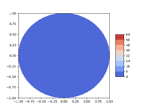
(a)

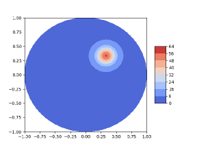
(b)

(c)

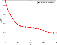
(d)

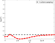
(e)

Figure 1: The first row shows media configurations (38), (39) for homogeneous and inhomogeneous media, respectively. The second row shows the landscape of the A-optimal objective (9) as a function of $L$ as in (40). For reference, the dashed lines are obtained from a uniform sampling distribution over the entire boundary $\partial\mathcal{D}^{2}$.

Figure 2 shows the landscape of the D-optimal objective criteria (10) on the homogeneous media, calculated in the same way as described above for $F^{A}$. (The plot of inhomogeneous case is close to Figure 2.) It can be seen the optimal $\rho_{L}$ in this case is achieved by setting $L=0$, indicating that voltage injection and intensity measurement should be placed at the same location. The comparison of this plot with Figure 1 also reminds us that different objective criterion can lead to different optimal solutions.

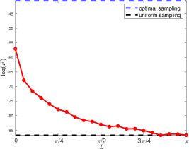
Figure 2: The landscape of D-optimal objective (10) for parameterized $\rho_{L}$ in (40). For reference, we plot the solution to both the optimal sampling strategy achieved by the classical Fedorov method [31, 40], and the uniform sampling.

6 Gradient flow for EIT design

We now describe the numerical performance of the particle gradient flow Algorithm 1, applied to the EIT problems whose media have different honogeneity properties and for which different initializations are used. We observe different convergence patterns for $\rho$ in different scenarios.

6.1 A-optimal design

We consider Algorithm 1 using the A-optimal objective function (9). Both the choice of $\mathbf{A}$ and the initial configuration affect the final equilibrium achieved by the flow. We define the initialization $\rho^{0}$ to be a uniform distribution supported on one of three regions:

1. entire design space;

2. restricted L-shape;

3. diagonal stripe.

(See Figure 3 for visualizations of the initialization.)

Remark 4.

In the numerical tests, the gradient flow Algorithm 1 does not converge to the same solution as starting from varied initialization measures. Such finding implies that the A- and D-OED landscapes may be nonconvex under the $W_{2}$ metric (5). We note that there is no contradiction of the $L_{2}$ convexity claim we showed in Proposition 4 of Section 4.2. The two different metrics and their convexity results are conceptually independent.

Note that the special design of Init.Item 2 assigns heavier weights to samples for which either $\theta_{1}$ or $\theta_{2}$ is in the sector $[0,\frac{\pi}{2}]$. Physically, this means that the particular region could carry more information, suggesting that it is a good place for sources and detectors.

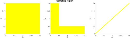
Figure 3: Initialization strategies for particle sampling: regions Init.Item 1, Init.Item 2, Init.Item 3, respectively.

We first examine the gradient information. Defining $\rho$ as in Init.Item 1, we compute:

$$\nabla_{\theta}\frac{\delta F^{A}[\rho]}{\delta\rho}\in\mathbb{R}^{2}\quad\eqref{eqn: A velocity}$$

as a function of $\theta=(\theta_{1},\theta_{2})$ over the design space. This function is plotted in Figure 4, with the top row showing results for homogeneous media $\mathbf{A}_{\mathrm{h}}$ and the bottom row showing those for inhomogeneous media $\mathbf{A}_{\mathrm{ih}}$.

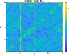
(a)

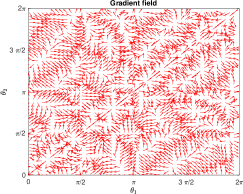
(b)

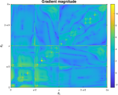
(c)

Figure 4: The gradients are computed via The results are computed using (17). (a) and (b) respectively shows the gradient magnitude and field for the homogeneous case $\mathbf{A}_{\mathrm{h}}.$ The red arrows in (b) indicate the gradient vector (17) directions. (c) shows the gradient magnitude for the inhomogeneous case $\mathbf{A}_{\mathrm{ih}}$.

For $\mathbf{A}_{\mathrm{h}}$, in (a) of Figure 4, the gradient magnitude is rather balanced over the entire design space, with relatively higher magnitude near the diagonal, where $\theta_{1}\approx\theta_{2}$. In contrast, from panel (c), $\mathbf{A}_{\mathrm{ih}}$ presents much stronger disparity in the gradient with the highest magnitude seen in the region of $(\theta_{1},\theta_{2})\in[0,\frac{\pi}{2}]^{2}$. We skip the gradient field of the inhomogeneous case since it is rather similar to the result in (b) Figure 4.

We now discuss the evolution of probability measure $\rho$ as Algorithm 1 proceeds, for different scenarios of media types and initializations. For gradient flow, the time discretization is set as $\differential t=2*10^{-7}$ and the total iteration number is $T=50.$ A periodic boundary condition is deployed in Algorithm 1. To be specific, in line 3 of Algorithm 1, the updated particle location follows $\theta$ is set to be $(\theta\mod 2\pi)$.

Init.Item 1 Init.Item 2 Init.Item 3 homogeneous maintain spread out the entire space maintain inhomogeneous concentrate in L-shape maintain

Table 1: Gradient flow convergence summary for A-optimal design. Rows represent media; columns represent the three initialization schemes.

Convergence results are summarized in Table 1. Further details, for the case of homogeneous media, are shown in Figure 5. Each row of figures shows one of the initialization schemes, with selected snapshots being shown in each case. For all initial sampling regimes, the objective values shown in the rightmost column keeps decaying till it saturates to a plateau, according to the gradient flow property. When the initial distribution is either uniform in the entire domain or in the $L$-shape area, the algorithm returns a distribution that spreads roughly over the entire region $[0,2\pi]^{2}$. We note frm panel (c) that the distribution concentrated along the diagonal seems to be a local minimum: If all samples are initially prepared in the diagonal stripe (Init.Item 3), the gradient flow only moves them along the diagonal, producing a probability distribution supported only on the diagonal $\theta_{1}\approx\theta_{2}$.

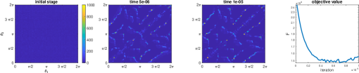
(a)

(b)

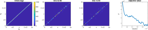
(c)

Figure 5: Homogeneous regime: Evolution of particle gradient flow Algorithm 1 under A-optimal criterion.

A similar study is conducted for the inhomogeneous media $\mathbf{A}_{\mathrm{ih}}$; see Figure 6. Similar to the homogeneous example, the objective function value $F^{A}$ decreases steadily. However, the final configurations are quite different from the homogeneous case. In the first row (Init.Item 1), particles initially sampled on the whole space tend towards the restricted L-shape part. In the second row (Init.Item 2), where the initial samples are confined in the L-shaped area already, they tend to stay in that region. These results suggest that either the source $\theta_{1}$ or the detector $\theta_{2}$ should be placed within the angle $[0,\pi/2],$ as this region delivers more information than the rest of the domain. Similar to the homogeneous media case, the sampling concentrated along the strip of $\theta_{1}=\theta_{2}$ appears to represent a local minimum, with an initial distribution with this property leading to subsequent iterates sharing the same property. (We omit the plots for this case.)

(a)

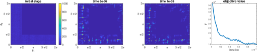
(b)

Figure 6: Inhomogeneous regime: evolution of particle gradient flow Algorithm 1 under A-optimal criterion.

6.2 D-optimal design

This section shows results of Algorithm 1 using the D-optimal design (10) criterion. We consider two types of initialization strategies for the distributions of the samples particles:

1. uniform distribution on the entire design space;

2. (approximately) optimal distribution provided by Fedorov method [31].

We first check the gradient direction field of D-optimal design in Figure 7. The gradient magnitude heatmap (left figure) shows particles concentrated in the diagonal area. The gradient field (right figure) shows that along a thin stripe of diagonal, the direction also tends to point along the diagonal, while outside the stripe, the gradient orientations are rather scattered.

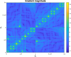
(a)

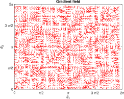
(b)

Figure 7: Gradient magnitude and direction field under D-optimal design criterion (10).

Finally, we show results for Algorithm 1, using flow simulation time step $\differential t=2*10^{-7}$ and $T=1000$ iterations. As shown in Figure 8(a), an initial uniform distribution of $\rho$ maintain uniformity during execution of Algorithm 1. While we cannot see much dissimilarity in the particle density map, the objective function keeps increasing throughout execution of Algorithm 1. In Figure 8(b), we run Algorithm 1 using the initialization provided by the Fedorov method. While again it is hard to tell the difference between the gradient flow equilibrium and the initial distribution, the D objective increases during execution of Algorithm 1 Meanwhile, the objective function $F^{A}$ decreases during execution for the first initialization, but not the second.

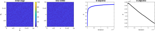
(a)

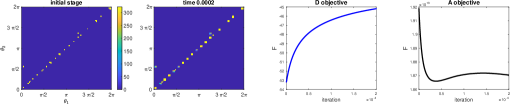
(b)

Figure 8: Evolution of particle gradient flow Algorithm 1 under D-optimal criterion, tested on the homogeneous media data $\mathbf{A}_{\mathrm{h}}$.

7 Conclusions

As computational techniques involving optimal transport and Wasserstein gradient flow become more mature, they offer the opportunity to deal with infinite-dimensional probability measure space, enabling a new and wider range of applications. The optimal experimental design (OED) problem in continuous design space is one such example, offering an important generalization over more traditional discrete experimental design.

The move from finite-dimensional Euclidean space to the infinite-dimensional probability manifold results in a more challenging optimization problem. We use newly available Wasserstein gradient flow techniques to recast the continuous OED problem. In particular, the gradient flow on measure space is mapped to gradient descent on a discrete set of particles representing the distribution in the Euclidean space. Algorithm 1 can be applied to solve the continuous OED. Moreover, we have provided the first criticality condition and basic convexity analysis under the A- and D-optimal design criteria. As a proof of concept, we assessed the algorithm’s performance on the EIT problem, observing convergence of Algorithm 1 to distributions that reveal interesting design knowledge on specific EIT media examples.

The present work opens the door to many additional questions, including the following.

1. Tensor structure in particle gradient flow Algorithm 1. If the design space $\Omega$ is high dimensional, it might be possible to decompose the particle update in Algorithm 1 and follow a multi-modal scheme. How to take advantage of such tensor structure to improve efficiency of the optimization process is one interesting direction to pursue.

2. Sensitivity to noise. It would be interesting to study sensitivity of the continuous OED optimizer to the noise encoded in the objective function and data.

3. Explicit error bound in the simulation. The currently available results still do not cover the entire rigorous numerical analysis. The roadmap was provided in Section 4.3. It would be interesting to fill in the missing technical arguments.

References

- [1] Alen Alexanderian, Philip J. Gloor, and Omar Ghattas. On Bayesian A- and D-Optimal Experimental Designs in Infinite Dimensions. Bayesian Analysis, 11(3):671 – 695, 2016.
- [2] Alen Alexanderian, Noemi Petra, Georg Stadler, and Omar Ghattas. A-optimal design of experiments for infinite-dimensional Bayesian linear inverse problems with regularized -sparsification. SIAM Journal on Scientific Computing, 36(5):A2122–A2148, 2014.
- [3] Alen Alexanderian, Noemi Petra, Georg Stadler, and Omar Ghattas. A fast and scalable method for A-optimal design of experiments for infinite-dimensional Bayesian nonlinear inverse problems. SIAM Journal on Scientific Computing, 38(1):A243–A272, 2016.
- [4] Alen Alexanderian and Arvind K Saibaba. Efficient D-optimal design of experiments for infinite-dimensional Bayesian linear inverse problems. SIAM Journal on Scientific Computing, 40(5):A2956–A2985, 2018.
- [5] Zeyuan Allen-Zhu, Yuanzhi Li, Aarti Singh, and Yining Wang. Near-optimal discrete optimization for experimental design: A regret minimization approach. Mathematical Programming, 186:439–478, 2021.
- [6] Luigi Ambrosio, Nicola Gigli, and Giuseppe Savaré. Gradient flows: in metric spaces and in the space of probability measures. Springer Science & Business Media, 2005.
- [7] Richard C Aster, Brian Borchers, and Clifford H Thurber. Parameter estimation and inverse problems. Elsevier, 2018.
- [8] Kendall E Atkinson. An Introduction to Numerical Analysis. John Wiley & Sons, 2008.
- [9] Ahmed Attia, Sven Leyffer, and Todd Munson. Robust A-optimal experimental design for Bayesian inverse problems. arXiv preprint arXiv:2305.03855, 2023.
- [10] Corwin L. Atwood. Optimal and Efficient Designs of Experiments. The Annals of Mathematical Statistics, 40(5):1570 – 1602, 1969.
- [11] Matt Avery, Harvey Thomas Banks, Kanadpriya Basu, Yansong Cheng, Eric Eager, Sarah Khasawinah, Laura Potter, and Keri L Rehm. Experimental design and inverse problems in plant biological modeling. 2012.
- [12] Haim Avron and Christos Boutsidis. Faster subset selection for matrices and applications. SIAM Journal on Matrix Analysis and Applications, 34(4):1464–1499, 2013.
- [13] Giovanni A Bonaschi, José A Carrillo, Marco Di Francesco, and Mark A Peletier. Equivalence of gradient flows and entropy solutions for singular nonlocal interaction equations in 1d. ESAIM: Control, Optimisation and Calculus of Variations, 21(2):414–441, 2015.
- [14] Liliana Borcea. Electrical impedance tomography. Inverse Problems, 18(6):R99, oct 2002.
- [15] S. Boyd and L. Vandenberghe. Convex Optimization. Cambridge University Press, 2003.
- [16] Tan Bui-Thanh, Omar Ghattas, James Martin, and Georg Stadler. A computational framework for infinite-dimensional Bayesian inverse problems part i: The linearized case, with application to global seismic inversion. SIAM Journal on Scientific Computing, 35(6):A2494–A2523, 2013.
- [17] Tan Bui-Thanh, Qin Li, and Leonardo Zepeda-Núnez. Bridging and improving theoretical and computational electrical impedance tomography via data completion. SIAM Journal on Scientific Computing, 44(3):B668–B693, 2022.
- [18] John Charles Butcher. Numerical methods for ordinary differential equations. John Wiley & Sons, 2016.
- [19] Alberto Calderón. On inverse boundary value problem. Computational & Applied Mathematics - COMPUT APPL MATH, 25, 01 2006.
- [20] José Antonio Carrillo, Yanghong Huang, Francesco Saverio Patacchini, and Gershon Wolansky. Numerical study of a particle method for gradient flows. arXiv preprint arXiv:1512.03029, 2015.
- [21] Ke Chen and Ruhui Jin. Tensor-structured sketching for constrained least squares. SIAM Journal on Matrix Analysis and Applications, 42(4):1703–1731, 2021.
- [22] Ke Chen, Qin Li, and Jian-Guo Liu. Online learning in optical tomography: a stochastic approach. Inverse Problems, 34(7):075010, 2018.
- [23] Ke Chen, Qin Li, Kit Newton, and Stephen J. Wright. Structured random sketching for pde inverse problems. SIAM Journal on Matrix Analysis and Applications, 41(4):1742–1770, 2020.
- [24] Lenaic Chizat and Francis Bach. On the global convergence of gradient descent for over-parameterized models using optimal transport. Advances in Neural Information Processing Systems, 31, 2018.
- [25] Emily Clark, Travis Askham, Steven L. Brunton, and J. Nathan Kutz. Greedy sensor placement with cost constraints. IEEE Sensors Journal, 19(7):2642–2656, 2019.
- [26] David A Cohn, Zoubin Ghahramani, and Michael I Jordan. Active learning with statistical models. Journal of Artificial Intelligence Research, 4:129–145, 1996.
- [27] Maarten V de Hoop, Nikola B Kovachki, Nicholas H Nelsen, and Andrew M Stuart. Convergence rates for learning linear operators from noisy data. SIAM/ASA Journal on Uncertainty Quantification, 11(2):480–513, 2023.
- [28] Michał Dereziński, Kenneth L Clarkson, Michael W Mahoney, and Manfred K Warmuth. Minimax experimental design: Bridging the gap between statistical and worst-case approaches to least squares regression. In Conference on Learning Theory, pages 1050–1069. PMLR, 2019.
- [29] Petros Drineas, Malik Magdon-Ismail, Michael W Mahoney, and David P Woodruff. Fast approximation of matrix coherence and statistical leverage. The Journal of Machine Learning Research, 13(1):3475–3506, 2012.
- [30] Otto Dykstra. The augmentation of experimental data to maximize [xx]. Technometrics, 13(3):682–688, 1971.
- [31] Valerii Vadimovich Fedorov. Theory of optimal experiments. Elsevier, 2013.
- [32] A. Figalli and F. Glaudo. An Invitation to Optimal Transport, Wasserstein Distances, and Gradient Flows. EMS textbooks in mathematics. European Mathematical Society, 2021.
- [33] Nicolas Fournier and Arnaud Guillin. On the rate of convergence in Wasserstein distance of the empirical measure. Probability theory and related fields, 162(3-4):707–738, 2015.
- [34] E Haber, L Horesh, and L Tenorio. Numerical methods for experimental design of large-scale linear ill-posed inverse problems. Inverse Problems, 24(5):055012, sep 2008.
- [35] Eldad Haber, Lior Horesh, and Linky Tenorio. Numerical methods for the design of large-scale nonlinear discrete ill-posed inverse problems. Inverse Problems, 26:025002 (14pp), 12 2009.
- [36] L. Horesh, E. Haber, and L. Tenorio. Optimal Experimental Design for the Large-Scale Nonlinear Ill-Posed Problem of Impedance Imaging, chapter 13, pages 273–290. John Wiley & Sons, Ltd, 2010.
- [37] Xun Huan and Youssef Marzouk. Gradient-based stochastic optimization methods in Bayesian experimental design. International Journal for Uncertainty Quantification, 4(6), 2014.
- [38] Xun Huan and Youssef M Marzouk. Simulation-based optimal Bayesian experimental design for nonlinear systems. Journal of Computational Physics, 232(1):288–317, 2013.
- [39] Jayanth Jagalur-Mohan and Youssef Marzouk. Batch greedy maximization of non-submodular functions: Guarantees and applications to experimental design. The Journal of Machine Learning Research, 22(1):11397–11458, 2021.
- [40] R. C. St. John and N. R. Draper. D-optimality for regression designs: A review. Technometrics, 17(1):15–23, 1975.
- [41] Mark E Johnson and Christopher J Nachtsheim. Some guidelines for constructing exact D-optimal designs on convex design spaces. Technometrics, 25(3):271–277, 1983.
- [42] Richard Jordan, David Kinderlehrer, and Felix Otto. The variational formulation of the Fokker–Planck equation. SIAM Journal on Mathematical Analysis, 29(1):1–17, 1998.
- [43] Samuel Karlin and William J Studden. Optimal experimental designs. The Annals of Mathematical Statistics, 37(4):783–815, 1966.
- [44] J. Kiefer. General Equivalence Theory for Optimum Designs (Approximate Theory). The Annals of Statistics, 2(5):849 – 879, 1974.
- [45] Andreas Krause, H Brendan McMahan, Carlos Guestrin, and Anupam Gupta. Robust submodular observation selection. Journal of Machine Learning Research, 9(12), 2008.
- [46] Vivek Madan, Mohit Singh, Uthaipon Tantipongpipat, and Weijun Xie. Combinatorial algorithms for optimal design. In Conference on Learning Theory, pages 2210–2258. PMLR, 2019.
- [47] Krithika Manohar, Bingni W Brunton, J Nathan Kutz, and Steven L Brunton. Data-driven sparse sensor placement for reconstruction: Demonstrating the benefits of exploiting known patterns. IEEE Control Systems Magazine, 38(3):63–86, 2018.
- [48] Toby J. Mitchell. An algorithm for the construction of “D-optimal” experimental designs. Technometrics, 42(1):48–54, 2000.
- [49] Ira Neitzel, Konstantin Pieper, Boris Vexler, and Daniel Walter. A sparse control approach to optimal sensor placement in PDE-constrained parameter estimation problems. Numerische Mathematik, 143(4):943–984, 2019.
- [50] Aleksandar Nikolov, Mohit Singh, and Uthaipon Tantipongpipat. Proportional volume sampling and approximation algorithms for A-optimal design. Mathematics of Operations Research, 47(2):847–877, 2022.
- [51] Noemi Petra, James Martin, Georg Stadler, and Omar Ghattas. A computational framework for infinite-dimensional Bayesian inverse problems, part ii: Stochastic Newton MCMC with application to ice sheet flow inverse problems. SIAM Journal on Scientific Computing, 36(4):A1525–A1555, 2014.
- [52] Gabriel Peyré, Marco Cuturi, et al. Computational optimal transport: With applications to data science. Foundations and Trends® in Machine Learning, 11(5-6):355–607, 2019.
- [53] Friedrich Pukelsheim. Optimal Design of Experiments. Society for Industrial and Applied Mathematics, 2006.
- [54] Lars Ruthotto, Julianne Chung, and Matthias Chung. Optimal experimental design for inverse problems with state constraints. SIAM Journal on Scientific Computing, 40(4):B1080–B1100, 2018.
- [55] Arvind K Saibaba, Alen Alexanderian, and Ilse CF Ipsen. Randomized matrix-free trace and log-determinant estimators. Numerische Mathematik, 137(2):353–395, 2017.
- [56] Filippo Santambrogio. Optimal Transport for Applied Mathematicians: Calculus of Variations, PDEs, and Modeling, volume 87. Birkhäuser, 2015.
- [57] Andrew I Schein and Lyle H Ungar. Active learning for logistic regression: an evaluation. Machine Learning, 68:235–265, 2007.
- [58] SD Silvey, DM Titterington, and B Torsney. An algorithm for D-optimal designs on a finite space. Report available from the authors, 1976.
- [59] Albert Tarantola. Inverse Problem Theory and Methods for Model Parameter Estimation. Society for Industrial and Applied Mathematics, 2005.
- [60] D Michael Titterington. Algorithms for computing D-optimal designs on a finite design space. In Proc. of the 1976 Conf. on Information Science and Systems, John Hopkins University, volume 3, pages 213–216, 1976.
- [61] B. Torsney and R. Martín-Martín. Multiplicative algorithms for computing optimum designs. Journal of Statistical Planning and Inference, 139(12):3947–3961, 2009.
- [62] Gunther Uhlmann. Electrical impedance tomography and calderón’s problem. Inverse problems, 25(12):123011, 2009.
- [63] Jean-Paul Watson, Harvey J Greenberg, and William E Hart. A multiple-objective analysis of sensor placement optimization in water networks, pages 1–10. 2004.
- [64] Keyi Wu, Peng Chen, and Omar Ghattas. A fast and scalable computational framework for large-scale high-dimensional Bayesian optimal experimental design. SIAM/ASA Journal on Uncertainty Quantification, 11(1):235–261, 2023.
- [65] Keyi Wu, Peng Chen, and Omar Ghattas. An offline-online decomposition method for efficient linear Bayesian goal-oriented optimal experimental design: Application to optimal sensor placement. SIAM Journal on Scientific Computing, 45(1):B57–B77, 2023.
- [66] Henry P Wynn. The sequential generation of -optimum experimental designs. The Annals of Mathematical Statistics, 41(5):1655–1664, 1970.
- [67] Henry P Wynn. Results in the theory and construction of D-optimum experimental designs. Journal of the Royal Statistical Society Series B: Statistical Methodology, 34(2):133–147, 1972.
- [68] Jing Yu, Victor Zavala, and Mihai Anitescu. A scalable design of experiments framework for optimal sensor placement. Journal of Process Control, 67, 04 2017.
- [69] Yaming Yu. D-optimal designs via a cocktail algorithm. Statistics and Computing, 21:475–481, 2011.
- [70] Victor M. Zavala. Stochastic optimal control model for natural gas networks. Computers & Chemical Engineering, 64:103–113, 2014.