Energy-level inversion for vortex states in spin-orbit coupled Bose-Einstein condensates

Abstract

We investigate vortex states in Bose-Einstein condensates under the combined action of the spin-orbit coupling (SOC), gradient magnetic field, and harmonic-oscillator trapping potential. The linear version of the system is solved exactly. Through the linear-spectrum analysis, we find that, varying the SOC strength and magnetic-field gradient, one can perform energy-level inversion. With suitable parameters, initial higher-order vortex states can be made the ground state (GS). The nonlinear system is solved numerically, revealing that the results are consistent with the linear predictions in the case of repulsive inter-component interactions. On the other hand, inter-component attraction creates the GS in the form of mixed-mode states in a vicinity of the GS phase-transition points. The spin texture of both vortex- and mixed-mode GSs reveals that they feature the structure of 2D (baby) skyrmions.

I Introduction

Atomic Bose-Einstein condensates (BECs) are versatile platforms for simulations of various phenomena from condensed-matter physics RepProgPhys.75.082401 ; Lewenstein . Among these phenomena, the spin-orbit coupling (SOC) plays a basic role in spin Hall effects RevModPhys.82.1959 , topological insulators RevModPhys.82.3045 , spintronic devices RevModPhys.76.323 , etc. The experimental realization of SOC in one-dimensional (1D) nature09887 ; Juzeliunas and two-dimensional (2D) Science.354.83 two-component BEC has inspired theoretical research into spin-orbit-coupled BECs. The analysis based on the Gross-Pitaevskii equations (GPEs) has produced remarkable phenomena, such as vortices Kawakami ; Drummond ; Sakaguchi ; PhysRevE.89.032920 ; PhysRevE.94.032202 ; CNSNS , solitons PhysRevLett.110.264101 ; 1D sol 2 ; 1D sol 3 ; 1D sol 4 ; Cardoso ; Lobanov ; 2D SOC gap sol Raymond ; SOC 2D gap sol Hidetsugu ; low-dim SOC ; Han Pu 3D , and skyrmions PhysRevLett.109.015301 . Comprehensive insights into experimental and theoretical achievements in this field are provided by review Spielman ; Galitski ; Ohberg ; Zhai ; SOC-sol-review ; Sherman .

2D solitons supported by the interplay of SOC and cubic attractive interactions in the free space are remarkable modes due to their stability against the collapse and specific vortex structure: depending on the relative strength of the cross- and self-attraction, stable modes are semi-vortices, with vorticities $0$ and $1$ in the two components, and mixed modes, which include terms with vorticities $\left(0,+1\right)$ in one component, and $\left(-1,0\right)$ in the other PhysRevE.89.032920 ; PhysRevE.94.032202 . However, semi-vortex and mixed-mode solitons are stable only when they represent the ground state (GS), while the corresponding excited states, produced by the addition of the equal vorticities to both components, are completely unstable. Stabilization of the higher-vorticity states can be provided if a tunable mechanism of energy-level inversion can be introduced, that modifies the eigen-energy spectrum while preserving the corresponding eigenfunctions. Ideally, it should enable the transformation of any higher-order vortex state into the GS, thereby paving the way for the experimental realization. Recently, a possibility of the transformation of any excited state into the respective GS in the 1D BEC with SOC and gradient magnetic field has been demonstrated in Ref. PhysRevA.106.063311 .

In this paper, we introduce the 2D SOC system which includes the gradient magnetic field and the harmonic-oscillator (HO) trapping potential. The linear version of the system is solved exactly. The solution demonstrates that the combined effect of SOC and magnetic field leads to reduction of the total energy of the vortex states, the size of the effect growing with the increase of the vorticity. Thus, by adjusting the SOC strength and magnetic-field gradient, one can realize the energy level inversion, making it possible to convert any higher-order vortex state into the GS. The full nonlinear system, including either repulsive or attractive inter-component interaction, is solved numerically.

The following presentation is structured as follows. The model is introduced in Sec. II. The linear solution is constructed in Sec. III, in terms of wave functions of Landau levels. In Secs. IV , numerical solutions of the nonlinear system with inter-component repulsion or attraction are produced. In Sec. V, spin textures of the newly found two-component states are presented in detail. The paper is concluded by Sec. VI.

II The model

We consider the spin-orbit-coupled effectively 2D binary BEC under the action of the HO trapping potential, written in the scaled form as $V=r^{2}/2$, and dc magnetic field $\mathbf{B}=(-\alpha x,-\alpha y,\Omega)$, which has a constant gradient $-\alpha$ along the $x$ and $y$ directions,while its $z$-component $\Omega$ is constant. The Rashba SOC is represented by operator $V_{\text{so}}=i\beta(\sigma_{y}\partial_{x}-\sigma_{x}\partial_{y})$ in the system of GPEs for the binary BEC, where $\mathbf{\sigma}=(\sigma_{x},\sigma_{y},\sigma_{z})$ is the vector of the Pauli matrices, and $\beta$ is the SOC strength. The scaled GPE system for the spinor wave function, $\Psi=(\Psi_{1},\Psi_{2})^{T}$, is

$$\begin{split}i\partial_{t}\Psi_{1}=&\frac{1}{2}\left(-\nabla^{2}+r^{2}\right)\Psi_{1}+\Omega\Psi_{1}-\alpha\left(x-iy\right)\Psi_{2}\\ &+\beta\left(\partial_{x}-i\partial_{y}\right)\Psi_{2}+\left(g|\Psi_{1}|^{2}+\gamma|\Psi_{2}|^{2}\right)\Psi_{1},\\ i\partial_{t}\Psi_{2}=&\frac{1}{2}\left(-\nabla^{2}+r^{2}\right)\Psi_{2}-\Omega\Psi_{2}-\alpha\left(x+iy\right)\Psi_{1}\\ &-\beta\left(\partial_{x}+i\partial_{y}\right)\Psi_{1}+\left(g|\Psi_{2}|^{2}+\gamma|\Psi_{1}|^{2}\right)\Psi_{2},\end{split}$$ (1)

where $\Omega$ plays the role of the effective Zeeman splitting between the components, $g$ and $\gamma$ are coefficients of the intra- and inter-component interactions, respectively 2D-magnetic-1 ; 2D-magnetic-2 ; 2D-magnetic-3 . Using the remaining scaling invariance of Eq. (1), we set $g=1$, assuming the repulsive sign of the self-interaction in each component. However, $\gamma$ may be negative, representing the possibility of the attraction between the components, which can be introduced by means of the Feshbach resonance Feshbach . For the use in the following analysis, we denote

$$\Omega\equiv\beta\Delta-\frac{1}{2},$$ (2)

where $\Delta$ serves as a tunable parameter employed to control the strength of Zeeman splitting.

Stationary solutions of Eq. (1) with chemical potential $\mu$ are sought for in the usual form,

$$\Psi(x,y,t)=\exp(-i\mu t)\{\psi_{1}(x,y),\psi_{2}(x,y)\}^{T},$$ (3)

with functions $\psi_{1,2}(x,y)$ satisfying equations

$$\begin{split}\mu\psi_{1}=&\frac{1}{2}\left(-\nabla^{2}+r^{2}\right)\psi_{1}+\Omega\psi_{1}-\alpha\left(x-iy\right)\psi_{2}\\ &+\beta\left(\partial_{x}-i\partial_{y}\right)\psi_{2}+\left(g|\psi_{1}|^{2}+\gamma|\psi_{2}|^{2}\right)\psi_{1},\\ \mu\psi_{2}=&\frac{1}{2}\left(-\nabla^{2}+r^{2}\right)\psi_{2}-\Omega\psi_{2}-\alpha\left(x+iy\right)\psi_{1}\\ &-\beta\left(\partial_{x}+i\partial_{y}\right)\psi_{1}+\left(g|\psi_{2}|^{2}+\gamma|\psi_{1}|^{2}\right)\psi_{2}~{}.\end{split}$$ (4)

The SOC system (1) conserves  two evident dynamical invariants, viz., the total norm of the two components,

$$N=\int\int\left[\left|\psi_{1}\left(x,y\right)\right|^{2}+\left|\psi_{2}\left(x,y\right)\right|^{2}\right]dxdy,$$ (5)

and energy (Hamiltonian),

$$\begin{split}E=&\iint\left\{\frac{1}{2}\!\left(\left|\nabla\psi_{1}\right|^{2}\!+\!\left|\nabla\psi_{2}\right|^{2}\right)\!+\!\frac{r^{2}}{2}\!\left(\left|\psi_{1}\right|^{2}+\left|\psi_{2}\right|^{2}\right)\right.\\ &-\alpha\left[\left(x-iy\right)\psi_{1}^{\ast}\psi_{2}+\left(x+iy\right)\psi_{1}\psi_{2}^{\ast}\right]\\ &-\beta\left[\psi_{2}\left(\partial_{x}-i\partial_{y}\right)\psi_{1}^{\ast}+\psi_{2}^{\ast}\left(\partial_{x}+i\partial_{y}\right)\psi_{1}\right]\\ &+\Omega\left(\left|\psi_{1}\right|^{2}-\left|\psi_{2}\right|^{2}\right)+\gamma\left|\psi_{1}\right|^{2}\left|\psi_{2}\right|^{2}\\ &\left.+\frac{g}{2}\left(\left|\psi_{1}\right|^{4}+\left|\psi_{2}\right|^{4}\right)\right\}dxdy,\end{split}$$ (6)

where $\ast$ stands for the complex conjugate. Note that the terms $\sim\beta$ in expression (6), which seem formally asymmetric with respect to $\Psi_{1}$ and $\Psi_{2}$, are actually symmetric, if one takes into regard the possibility of the application of integration by parts, $\Psi_{2}\left(\partial_{x}-i\partial_{y}\right)\Psi_{1}^{\ast}\rightarrow-\Psi_{1}^{\ast}\left(\partial_{x}-i\partial_{y}\right)\Psi_{2}$. The system’s GS corresponds to a minimum of the energy for a fixed value of the norm. In fact, for the linearized system, with $g=\gamma=0$, the energy of stationary states is proportional to the respective chemical potential, determined by the stationary GPE system (4), therefore, in the linear limit, the energy minimization is tantamount to the minimization of $\mu$.

We note that, in terms of polar coordinates $\left(r,\theta\right)$ and wave-function components

$$\tilde{\Psi}_{1}\equiv\Psi_{1},\tilde{\Psi}_{2}\equiv e^{-i\theta}\Psi_{2},$$ (7)

expression (6) for the energy takes an axisymmetric form:

$$\begin{split}E=&\int_{0}^{\infty}rdr\int_{0}^{2\pi}d\theta\left\{\frac{1}{2}\sum_{j=1,2}\left(\left|\frac{\partial\tilde{\psi}_{j}}{\partial r}\right|^{2}+\frac{1}{r^{2}}\left|\frac{\partial\tilde{\psi}_{j}}{\partial\theta}\right|^{2}\right)\right.\\ &+\frac{r^{2}}{2}\left(\left|\tilde{\psi}_{1}\right|^{2}+\left|\tilde{\psi}_{2}\right|^{2}\right)-\alpha r\left(\tilde{\psi}_{1}^{\ast}\tilde{\psi}_{2}+\tilde{\psi}_{1}\tilde{\psi}_{2}^{\ast}\right)\\ &-\beta\left[\tilde{\psi}_{2}\left(\frac{\partial}{\partial r}-\frac{i}{r}\frac{\partial}{\partial\theta}\right)\tilde{\psi}_{1}^{\ast}+\tilde{\psi}_{2}^{\ast}\left(\frac{\partial}{\partial r}+\frac{i}{r}\frac{\partial}{\partial\theta}\right)\tilde{\psi}_{1}\right]\\ &+\Omega\left(\left|\tilde{\psi}_{1}\right|^{2}-\left|\tilde{\psi}_{2}\right|^{2}\right)+\gamma\left|\tilde{\psi}_{1}\right|^{2}\left|\tilde{\psi}_{2}\right|^{2}\\ &\left.+\frac{g}{2}\left(\left|\tilde{\psi}_{1}\right|^{4}+\left|\tilde{\psi}_{2}\right|^{4}\right)\right\}.\end{split}$$ (8)

The invariance of energy (8) with respect to the rotation by arbitrary angle, $\theta\rightarrow\theta+\delta\theta$, implies that the additional dynamical invariant of the system is the angular momentum, which is defined as

$$\begin{split}M=&\int\int\left(\tilde{\psi}_{1}^{\ast}\hat{L}\tilde{\psi}_{1}+\tilde{\psi}_{2}^{\ast}\hat{L}\tilde{\psi}_{2}\right)dxdy\\ \equiv&\int\int\left[\psi_{1}^{\ast}\hat{L}\psi_{1}+\psi_{2}^{\ast}\left(\hat{L}-1\right)\psi_{2}\right]dxdy,\end{split}$$

where $\hat{L}=i\left(y\partial_{x}-x\partial_{y}\right)\equiv-i\partial_{\theta}$ is the canonical angular-momentum operator.

It is relevant to mention that essentially the same GPE system (1) can be derived if, instead of the real magnetic field, a synthetic field is used. It is well known that synthetic magnetic fields can be induced by rapid rotation of the condensate Cornell , or by an appropriate combination of illuminating laser beams Spielman-2 . The use of synthetic fields opens the way to realization of many fascinating phenomena, such as the Dirac’s monopole monopole .

Equations (1) and (4) are written in the scaled form. In physical units, assuming that the binary condensate is a mixture of two different atomic states of ⁸⁷Rb nature09887 , a relevant value of the HO trapping frequency is $\omega=10$ Hz. The number of atoms in the condensates is $1000$, which is sufficient for the experimental observation of the predicted patterns in full detail. The characteristic length, time and energy are identified as $l=\sqrt{\hbar/m_{\mathrm{at}}\omega}=8.55$ $\mathrm{\mu}$m, $\tau=1/\omega=100$ ms, and $\epsilon=\hbar\omega=1.05\times 10^{-33}$ J, where $m_{\mathrm{at}}=1.44\times 10^{-25}$ kg is the atomic mass of ⁸⁷Rb. The strength of SOC, denoted by $\beta=l\pi/\left(\sqrt{3}\lambda\right)$, where $\lambda$ represents the wavelength of the laser, can be adjusted across a wide range depending on the specific configurations of the laser system BEC-SOC GP eqns . Moreover, the shorter the wavelength of the laser, the greater the SOC strength. For instance, the Nd:YAG lasers typically emit light with a wavelength of 1064 nm, corresponding to a SOC strength of $\beta=1.47$, while the He-Ne lasers emit light with a wavelength of 633 nm, resulting in a higher SOC strength of $\beta=2.45$.

III The solution of the linear system

We first solve the linear version of Eq. (4), i.e.,

$$\hat{H}\psi\!=\!\mu\psi,$$ (9)

where the Hamiltonian can be represented in the compact form,

$$\hat{H}\!=\!\begin{bmatrix}\hat{a}^{\dagger}\hat{a}+\hat{b}^{\dagger}\hat{b}+\frac{1}{2}+\beta\Delta&(\beta-\alpha)\hat{b}-(\alpha+\beta)\hat{a}^{\dagger}\\ (\beta-\alpha)\hat{b}^{\dagger}-(\alpha+\beta)\hat{a}&\hat{a}^{{\dagger}}\hat{a}+\hat{b}^{{\dagger}}\hat{b}+\frac{3}{2}-\beta\Delta\end{bmatrix},$$ (10)

where the creation and annihilation operators are introduced as $\hat{a}^{\dagger}=(x-iy-\partial_{x}+i\partial_{y})/2$, $\hat{a}=(x+iy+\partial_{x}+i\partial_{y})/2$, $\hat{b}^{\dagger}=(x+iy-\partial_{x}-i\partial_{y})/2$ and $\hat{b}=(x-iy+\partial_{x}-i\partial_{y})/2$. To solve the linear stationary Schrödinger equation (9), a series of wave functions of the Landau levels are introduced as the basis LL :

$$\begin{split}&f_{n,m}(r,\theta)\\ &=\frac{\exp\left(im\theta-r^{2}/2\right)}{\sqrt{\pi n!(n+m)!}}\sum_{k=0}^{n+m}C_{n+m}^{k}A_{n}^{k}(-1)^{k}r^{2(n-k)+m},\end{split}$$ (11)

where $m$ is the winding number (alias vorticity, or magnetic quantum number), $n$ is an auxiliary quantum number, and $n+m$ is the Landau-level index. The ranges of $n$ and $m$ are $n=0,1,2,\ldots$ and $m=-n,-n+1,-n+2,\ldots$, respectively ($m$ also takes positive integer values). $C_{n}^{m}=\frac{n!}{m!(n-m)!}$ are the binomial coefficients, and $A_{n}^{m}=\frac{n!}{(n-m)!}$ for $m\leq n$; $A_{n}^{m}\equiv 0$ for $m>n$. The action of operators $\hat{b}^{\dagger}$ and $\hat{a}^{\dagger}$ on wave function (11) amounts to

$$\begin{array}[]{ll}\hat{a}^{\dagger}f_{n,m}=\sqrt{n+1}f_{n+1,m-1},&\hat{a}f_{n,m}=\sqrt{n}f_{n-1,m+1},\\ \hat{b}^{\dagger}f_{n,m}=\sqrt{n+m+1}f_{n,m+1},&\hat{b}f_{n,m}=\sqrt{n+m}f_{n,m-1}.\end{array}$$ (12)

In the case of equal SOC and magnetic-field-gradient coefficients in Eqs. (1) and (4), $\alpha=\beta$, the present linear system (9) admits an exact solution (eigenstate), in terms of wave functions (11),

$$\begin{split}\psi_{1}^{n,m}&=\frac{1}{\sqrt{\mathcal{N}_{n}}}f_{n,m}(r,\theta),\\ \psi_{2}^{n,m}&=\frac{\sqrt{4n+\Delta^{2}}+\Delta}{2\sqrt{\mathcal{N}_{n}n}}f_{n-1,m+1}(r,\theta),\end{split}$$ (13)

where $\Delta$ is defined by Eq. (2), and the normalization coefficient is

$$\mathcal{N}_{n}=\left\{\begin{array}[]{ll}1,&n=0,\\ \displaystyle\frac{4n+\Delta^{2}+\Delta\sqrt{4n+\Delta^{2}}}{2n},&n=1,2,3,\ldots~{}.\end{array}\right.$$ (14)

The difference $\delta m=1$ between the two components of eigenstate (13) is a characteristic feature of bound states of the above-mentioned semi-vortex type supported by SOC in the 2D space PhysRevE.89.032920 . The corresponding eigenvalues of the chemical potential are

$$\mu_{n,m}=\left\{\begin{array}[]{ll}\frac{1}{2}+m+\beta\Delta,&n=0,\\ \frac{1}{2}+2n+m-\beta\sqrt{4n+\Delta^{2}},&n=1,2,3,\ldots~{}.\end{array}\right.$$ (15)

For given quantum number $n$, the eigenvalues (15) attain a minimum at $m=-n$, namely,

$$\mu_{n,m=-n}\equiv\mu_{n}=\left\{\begin{array}[]{ll}\frac{1}{2}+\beta\Delta,&n=0,\\ \frac{1}{2}+n-\beta\sqrt{4n+\Delta^{2}},&n=1,2,3,\ldots{}\end{array}\right.$$ (16)

(however, this conditional minimum, corresponding to a particular value of $n$, does not imply the system’s GS, which should be identified as the absolute minimum). The respective wave function is

$$\begin{split}\psi_{1}^{n,m=-n}&=R_{1}^{(n)}(r)\exp(-in\theta),\\ \psi_{2}^{n,m=-n}&=R_{2}^{(n)}(r)\exp\left[-i(n-1)\theta\right],\end{split}$$ (17)

where the radial wave functions $R_{1,2}^{(n)}$ for $n\geq 1$ are

$$\begin{split}R_{1}^{(n)}&=\frac{1}{\sqrt{\pi n!\mathcal{N}_{n}}}r^{n}\exp\left(-\frac{r^{2}}{2}\right),\\ R_{2}^{(n)}&=\frac{\sqrt{4n+\Delta^{2}}+\Delta}{2\sqrt{\pi n!\mathcal{N}_{n}}}r^{{n}-1}\exp\left(-\frac{x^{2}}{2}\right),\end{split}$$ (18)

and for $n=0$,

$$R_{1}^{(0)}=(1/\sqrt{\pi})\exp(-r^{2}/2),~{}R_{2}^{(0)}=0.$$ (19)

Typical profiles of the radial wave functions are plotted in Figs. 1(a-c).

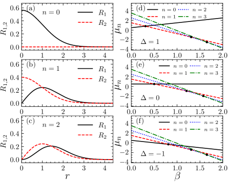
Figure 1: (a)-(c): Profiles of the radial wave functions $R_{1,2}^{(n)}(r)$, defined as per Eqs. (18) and (19), with quantum numbers (a) $n=0$, (b) $n=1$ and (c) $n=2$. (d)-(f): The corresponding chemical potential $\mu_{n}(\beta)$ with (d) $\Delta=1$, (e) $\Delta=0$, and (f) $\Delta=-1$, plotted pursuant to Eq. (16). The dots are values of $\beta_{n}$ defined by Eq. (20).

Thus, the quantum number $n=-m$ can be used to label the order of vortex states (17). It is seen that the SOC strength $\beta$ alters the spectrum (16) of eigenvalues $\mu_{n}$, but does not affect the corresponding eigenfunctions (18). In particular, Figs. 1(d-f) display the dependence of $\mu_{n}$ (alias energy, as it is proportional to the chemical potential for the linearized system) on $\beta$ at $\Delta=0$ and $\pm 1$. Branches $\mu_{n}$ with larger numbers $n$ vary faster as functions of $\beta$. The intersection of the branches corresponding to values $n$ and $n+1$ implies the GS switching. The respective critical values $\beta_{n}$ at the switching points can be obtained by solving equation $\mu_{n}(\beta_{n})=\mu_{n+1}(\beta_{n})$:

$$\beta_{n}\!=\!\frac{1}{4}\left\{\begin{array}[]{ll}\vspace{0.1cm}\displaystyle\sqrt{4+\Delta^{2}}-\Delta,&n=0,\\ \displaystyle\sqrt{4n+4+\Delta^{2}}+\sqrt{4n+\Delta^{2}},&n=1,2,\ldots~{}.\end{array}\right.$$ (20)

Thus we find the fact that vortex states with any order $n$ can become the system’s GS by adjusting the value of the SOC strength $\beta$.

The above analysis is based on the special case of $\alpha=\beta$ (equal SOC and magnetic-field-gradient strengths). The analysis can be extended for $\alpha\neq\beta$, setting $\Delta=0$ in Eq. (9), i.e., $\Omega=-1/2$ in Eq. (1). Then, an approximate solution of Eq. (9) with winding number $m$ (alias magnetic quantum number) can be looked for as a combination of the Landau-level wave functions truncated at $n=N_{t}$:

$$\begin{split}\psi_{1}&=\sum_{n=0}^{N_{t}}c_{n}f_{n,m},\\ \psi_{2}&=\sum_{n=0}^{N_{t}}d_{n}f_{n-1,m+1},\end{split}$$ (21)

where $c_{n}$ and $d_{n}$ are coefficients to be determined. We here produce the approximate results for $N_{t}=50$, which are practically exact. By substituting the ansatz (21) into Eq. (9) , we derive a set of coupled linear equations for $c_{n}$ and $d_{n}$:

$$\begin{split}\mu c_{n}&=\left(2n+m+\frac{1}{2}\right)c_{n}-(\alpha+\beta)\sqrt{n}d_{n}\\ &+(\beta-\alpha)\sqrt{n+m+1}d_{n+1},\\ \mu d_{n}&=\left(2n+m+\frac{1}{2}\right)d_{n}-(\alpha+\beta)\sqrt{n}c_{n}\\ &+(\beta-\alpha)\sqrt{n+m}c_{n-1}.\end{split}$$ (22)

Once the quantum number $m$ is fixed, Eq. (22) can be solved by dint of numerical diagonalization of the corresponding matrix. By comparing the chemical potentials $\mu$ corresponding to different winding numbers $m$, we can thus identify the system’s GS.

The so produced map of quantum numbers $m$, corresponding to the GS, in the $(\alpha,\beta)$ parameter plane (alias the GS phase diagram) is plotted in Fig. 2. Along the diagonal, $\alpha=\beta$, the GS predicted by this diagram agrees with the exact one given by Eq. (20) (note the symmetry about the diagonal). The phase diagram demonstrates that the GS switching between quantum numbers $m$ and $m+1$ takes place at $\alpha\neq\beta$ as well. Furthermore, we find that if fixing $\beta=3.0$, as $\alpha$ changes from negative to positive, the quantum number $m$ gradually transitions from positive to negative. Due to the symmetric structure of states with quantum numbers $m$ and $-m$, we focused only on the case where $m\leq 0$, or in other words, the case where $\alpha\geq 0$.

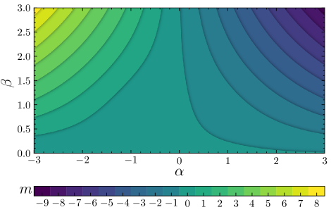
Figure 2: The map of values of the winding number (magnetic quantum number) $m$ corresponding to GS of the linear system in the ($\alpha,\beta$) parameter plane.

IV The numerical solution for the nonlinear system

We address the complete form of Eq. (4), including the nonlinear terms, repulsive or attractive, while fixing $\alpha=\beta$, as in the exact solution of the linear system. While energy-level inversion can be achieved by changing both the parameters $\Delta$ and $\beta$, altering $\Delta$ also changes the wave functions of each energy level, whereas altering $\beta$ does not affect the wave functions. To focus on the manipulations of the spectrum, in the following discussion, we vary $\beta$ while keeping $\Delta=0$. In this case, stationary states can be found in the numerical form by means of the imaginary-time propagation method Bao , fixing the total norm of the solution as $N=1$, see Eq. (5). The input which was used to generate the solutions by means of this method was taken as a superposition of the vortex components of the linear eigenmodes given by Eqs. (17) and (18), viz.,

$$\psi_{1}=\psi_{2}=\sum_{n=0}^{N_{s}}\frac{r^{n}\exp(-in\theta-r^{2}/2)}{\sqrt{2\pi N_{s}}}.$$ (23)

For numerical calculations with $0\leq\beta\leq 2$, choosing $N_{s}=5$ in Eq. (23) is sufficiently to generate stable eigenmodes of the nonlinear system.

We dwell on four cases, $\gamma=1$, $\gamma=0$, $\gamma=-1$, and $\gamma=-2$, which correspond, respectively, to the repulsive, zero, attraction and stronger attraction between the components. Note that the commonly known miscibility condition for the binary Bose gas in the free space is, in the present notation, $\gamma<1$ Mineev . The case of $\gamma=1$ corresponds to the miscibility boundary, but the pressure if the OH trapping potential induces effective miscibility in this case.

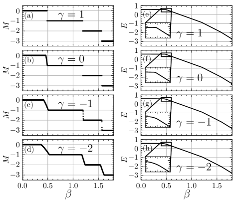
Figure 3: (a-d) Angular momentum $M$ and (e-h) energy $E$, defined as per Eqs. (II) and (6), respectively, as produced by the imaginary-time simulations of the full (nonlinear) system (1), for $\beta$ varying from $0$ to $1.8$, with step $\delta\beta=0.001$, at (a, e) $\gamma=1$, (b, f) $\gamma=0$, (c, g) $\gamma=-1$ and (d, h) $\gamma=-2$.

The stationary nonlinear states may be naturally quantified by the angular momentum (II). It is easy to check $M=m$ if one substitutes eigenfunction (13) into Eq. (II). Thus, integer values of $M$ indicate vortex (or semi-vortex PhysRevE.89.032920 ) states, while non-integer values of $M$ indicate mixed-mode states, defined as in Ref. PhysRevE.89.032920 . The dependence of $M$ on $\beta$, produced by the numerical solution is shown in Fig. 3.

For the different values of $\gamma$, dependences $M(\beta)$ in Fig. 3 (a-d) exhibit similar patterns, except in the vicinity of the phase-transition points. Recall that the GS phase transitions in the exact solution for the linear system are given by Eq. (20) – in particular, $\beta_{0}=0.5$, $\beta_{1}=1.2$, and $\beta_{2}=1.6$. As $\beta$ increases, $M$ follows the descending staircase-like pattern, dropping by $1$ while passing each phase transition. Flat segments of the $M(\beta)$ dependences are populated by the (semi-)vortex two-component states, see typical examples in Fig. 4, while the oblique transition segments carry mixed-mode states, see examples in Fig. 5. Parameter $\gamma$ affects the width of the phase-transition region, which is wider for smaller value of $\gamma$, in agreement with the general trend to stabilization of mixed modes and destabilization of semi-vortices following the decrease of $\gamma$ (increase of $-\gamma$) PhysRevE.89.032920 .

Curves for energy $E$ as a function of $\beta$ are plotted in Fig. 3 (e-h). We can find that as $\gamma$ decreases, the curves near the phase transition point gradually become smoother. For regions far from the phase transition point, these curves are similar for different values of $\gamma$. Energy $E$ gradually decreases with the increase of $\beta$. Furthermore, each time that $\beta$ passes a phase-transition point, the rate of energy reduction accelerates. These results are similar to those for the dependences $\mu_{n}(\beta)$ of the chemical potenital displayed in Eq. (16), which is actually the energy of the linearized system.

To quantitatively analyze the impact of different $\gamma$ on the total energy of the vortex state, we utilized the linear solutions given by Eqs. (17) and (18) as an approximation for the nonlinear system. This approach yielded the energy induced by inter-component interactions for $n\geq 1$ as expressed by the equation:

$$E_{\text{xpm}}=2\pi\gamma\int_{0}^{\infty}|R^{n}_{1}(r)|^{2}|R^{n}_{2}(r)|^{2}rdr=\frac{\gamma C_{2n}^{n}}{2^{2n+3}\pi}.$$ (24)

Additionally, for the case where $n=0$, the energy $E_{\text{xpm}}$ is equal to 0. For the situations we discussed above, namely, $n=0,1,2$ and 3, the corresponding $E_{\text{xpm}}=0$, $0.020\gamma$, $0.015\gamma$ and $0.012\gamma$, respectively. This result indicates that the total energy of the system remains very close under different $\gamma$ values.

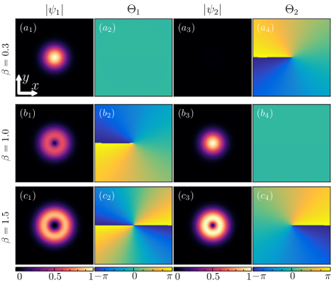
Figure 4: Distributions of the absolute values, $\left|\psi_{1,2}\right|$, and phases, $\Theta_{1,2}$, of wave functions of the two components in the GS of the (semi-) vortex type, for $\beta=0.3$ (panels $a_{1}-a_{4}$, with vorticities $0$ and $+1$ in the two componets; panel $a_{3}$ seems as an empty one, as $\left|\psi_{2}\right|$ is very small in that case); $\beta=1.0$ (panels $b_{1}-b_{4}$, with vorticities $-1$ and $0$); and $\beta=1.5$ (panels $c_{1}-c_{4}$, with vorticities $-2$ and $-1$). Other parameters in Eq. (1) are $\Delta=0$ and $\gamma=1$.

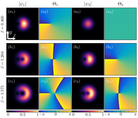
Figure 5: Distributions of the absolute values, $\left|\psi_{1,2}\right|$, and phases, $\Theta_{1,2}$, of wave functions of the two components in the GS of the mixed-mode type for $\beta=0.460$ (panels $a_{1}-a_{4}$), $\beta=1.204$ (panels $b_{1}-b_{4}$), $\beta=1.575$ (panels $c_{1}-c_{4}$), and $\Delta=0$, $\gamma=-2$ in Eq. (4).

As concerns the (semi-) vortex GSs displayed in Fig. 4 for $\gamma=1$, those for $\beta=0.3$, $1.0$, and $1.5$ correspond, severally, to values of the angular momentum (II) $M=0$, $-1$, and $-2$, as is seen from comparison with Fig. 3. These properties are readily explained by the fact that in all these cases an absolute majority of atoms belong to component $\psi_{1}$, which has the same values of intrinsic vorticities, viz., $m=0$,$-1$, and $-2$, respectively. Thus, selecting appropriate values of $\beta$, it is possible to adjust the vortex GS so as to realize any desirable value of its winding number.

On the other hand, the set of mixed-mode GSs found in the case of the inter-component attraction ($\gamma=-2$), which are displayed in Fig. 5, have half-integer values of angular momentum (II), viz., $M(\beta=0.460)=-0.5$, $M(\beta=1.204)=-1.5$, and $M(\beta=1.575)=-2.5$. These values of $M$ are explained by the fact that the corresponding mixed states are composed of two components with vorticities $m\leq-1$ and $m+1$, which have equal weights (this is a generic property of mixed-mode solitons in the free 2D space). Further, particular panels in Fig. 5 demonstrate an essential difference of the mixed-mode GSs from their counterparts of the (semi-)vortex type: in the mixed modes, higher-order vortices with $|m|\geq 2$ tend to split in lower-order ones, with separated pivots, and the pivots shift sidewise. The evolution of the mixed-mode GSs can be summarized as follows: as $\beta$ increases, the next phase transition increases the winding number of the right vortex in the $\psi_{1}$ component by $1$, while $\psi_{2}$ assumes a shape similar to that featured by the mixed-mode’s $\psi_{1}$ component at the previous stage.

To corroborate that the GSs, identified by the above analysis, are indeed stable modes, as they should be, their stability was verified by real-time simulations of their perturbed evolution. We added white noise to the ground state wave functions, with the maximum noise intensity reaching $10\%$ of the wave function’s amplitude. Subsequently, real-time evolution was applied to the perturbed wave functions. The results of numerical simulations are presented in Fig. 6, showcasing a vortex state with parameters $\beta=1.5$, $\gamma=1$, and a mixed state with parameters $\beta=1.575$, $\gamma=-2$. It can be seen that at $t=0$, the wave functions exhibit numerous noise points. However, as time progresses, by $t=200$, the noise points on the wave functions disappear. Furthermore, in the subsequent evolution, the phases of the wave functions rotate around the vortex centers, while the amplitude distribution no longer undergoes changes. The results completely verify the stability of the ground states in all cases.

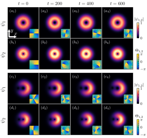
Figure 6: Numerical evolution of the perturbed ground state, where ($a_{1}-a_{4}$) and ($b_{1}-b_{4}$) correspond to vortex state with parameters $\beta=1.5$, $\gamma=1$, while ($c_{1}-c_{4}$) and ($d_{1}-d_{4}$) correspond to mixed state with parameters $\beta=1.575$, $\gamma=-2$. In each figure, the bottom right corner depicts the phase distribution of the wave function. From left to right, each column corresponds to the wave function density and phase distribution at evolution times $t=0$ (initial state), $t=200$, $t=400$, and $t=600$.

V The (semi-)vortex and mixed states as baby skyrmions

The realization of SOC in the two-component Bose gas suggests that it can be considered as a (pseudo-)spin system, with the spin vector density defined as

$$\mathbf{S}=\left(\psi^{\dagger}\psi\right)^{-1}\psi^{\dagger}\mathbf{\sigma}\psi.$$ (25)

For the vortex states with winding number $m\neq 0$ [recall $m=-n$, as in Eq. (17)], vector $\mathbf{S}$ produced by the linear solution (18) is

$$\mathbf{S}(r,\theta)=\frac{1}{r^{2}+1}\left\{2r\cos\theta,2r\sin\theta,r^{2}-1\right\}.$$ (26)

For $m=0$, the spin-vector structure is trivial, $\mathbf{S}(r,\theta)=\left\{0,0,1\right\}$.

The spin textures of the vortex states with winding numbers $m=0,-1$ and $-2$ in the $\psi_{1}$ component are displayed in Fig. 7(a-c). These textures for the states with $m\neq 0$ resemble those for 2D skyrmions, which are often called “baby skyrmions” (to stress the difference from their full-fledged 3D counterparts). The “babies” are well-known nonlinear modes Bogolyub ; Piette ; Yasha ; baby-opt which, in particular, were recently created in BEC baby-BEC .

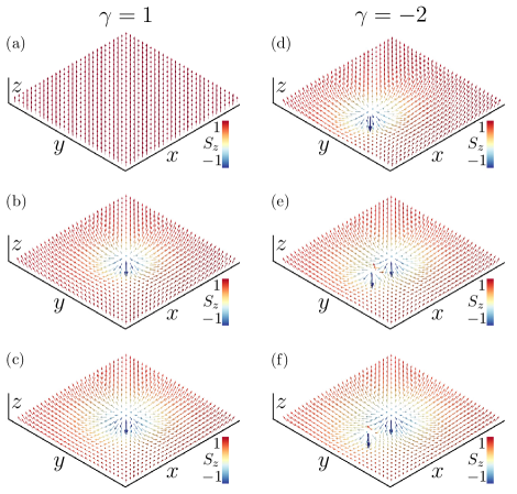
Figure 7: Spin textures of the numerically constructed GSs of the (a-c) vortex and (d-f) mixed-mode states in the nonlinear system with $\gamma=1$ and $\gamma=-2$, respectively. The vortex GSs in panels (a-c) are identical to those displayed in Fig. 4, with the same parameters, viz., $\beta=0.3$ and vorticities of the two components $\left(0,+1\right)$ (a), $\beta=1.0$ and vorticities $\left(-1,0\right)$ (b), and $\beta=1.5$ and vorticities $\left(-2,-1\right)$ (c). Similarly, the mixed-mode GSs in panels (d-f) are identical to those displayed in Fig. 5, with the same parameters, viz., $\beta=0.460$ (a), $\beta=1.204$ (b), and $\beta=1.575$ (c). Arrows indicate the direction of the spin vector (25), and their colors represent the magnitude of the $S_{z}$ component. Accordingly, the respective directions vary from vertical-up (red) to vertical-down (blue) ones. Bold blue arrows indicate the cores of the vortices.

According to Eq. (26), $\lim_{r\rightarrow\infty}\mathbf{S}=\left\{0,0,1\right\}$, hence the skyrmionic spin textures are embedded in the asymptotically uniform vector background. Thus, the 2D space $\mathbb{R}^{2}$ may be compactified into the 2D sphere $S^{2}$. Note that spin vectors (26) also take their values on $S^{2}$, therefore the skyrmion realizes the second homotopy group $\pi_{2}(S^{2})=\mathbb{Z}$, characterized by the topological number

$$Q=\frac{1}{4\pi}\int_{-\infty}^{\infty}\int_{-\infty}^{\infty}\mathbf{S}\cdot\left(\frac{\partial\mathbf{S}}{\partial x}\times\frac{\partial\mathbf{S}}{\partial y}\right)dxdy.$$ (27)

The skyrmion topological number counts the number of times that $S^{2}$ is covered by the vector field $\mathbf{S}(r,\theta)$. The substitution of expression (26) in Eq. (27) yields $Q=-1$, which is the topological charge of all the vortex states with $m\neq 0$, produced by the linear and nonlinear versions of Eq. (4) alike. In particular, the numerical calculation of topological charge $Q$ according to Eq. (27), for states displayed in panels (a-c) in Fig. 7, yields $Q(m=0)=4.049\times 10^{-4},Q(m=-1)=-0.978$, and $Q(m=-2)=-0.962$, respectively, in agreement with what is said above. Here the numerical-integration domain is $0\leq r<8.0,0\leq\theta<2\pi$. According to Eq. (27), numerical integration over the entire space, i.e., $-\infty<x,y<\infty$, is inherently challenging, and there is always a presence of systematic error. Increasing the integration range, while maintaining a constant spacing between the sampled points ($dxdy$), would indeed yield topological numbers $Q$ closer to integers. However, this approach necessitates significantly higher computational resources.

The mixed-mode states can be considered as a (nonlinear) superposition of two baby-skyrmions with topological charges $Q=0$ and $-1$. The spin textures of the mixed modes are presented in Figs. 7 (d-f), and the respective numerically calculated values of topological charge (27) are $Q=-0.980,-1.931$ and $-1.891$, respectively. The corresponding values for the ideal solutions are $Q=-1,-2$, and $-2$, respectively.

To visualize the structure of the skyrmions, it is relevant to identify location of vortex core(s) in them, i.e., points where vector (26) take the value $\mathbf{S}=\left\{0,0,-1\right\}$. The vortex states with $m\neq 0$, displayed in Figs. 4 and 7(a-c), feature the single core, pinned to the center, $r=0$. On the other hand, Figs. 5 and 7(d-f) show that (as is actually mentioned above) for the first mixed-mode state, the core position is offset from the center, and two cores are featured by the second and third mixed modes.

VI Conclusion

In this work, we have reported results of the systematic analysis of vortex states in the 2D SOC (spin-orbit-coupled) BEC under the action of the gradient magnetic field and HO trapping potential. We have obtained exact solutions for the linearized system and found that, by varying the SOC strength and the magnetic-field gradient, the energy-level inversion can be realized, allowing the trapped higher-order vortex modes to transition into the GS (ground state). We have also solved the full nonlinear system numerically and found that, in the case of the inter-component repulsion, the results for the vortex modes are consistent with the predictions of the linear theory. On the other hand, the attractive inter-component interaction creates mixed-mode states in the vicinity of the GS phase-transition points. Then, we have analyzed the GS spin textures and found that both the vortex and mixed-mode states have the structure of the 2D (baby) skyrmions. Our findings predict possibilities for the creation of stable higher-order vortex states in experiments with BEC.

It may be relevant to elaborate similar settings, emulating the SOC and the action of gradient magnetic field, in optics. A challenging possibility is to extend the analysis for 3D systems, cf. Ref. Han Pu .

References

- (1) P. Hauke, F. M. Cucchietti, L. Tagliacozzo, I. Deutsch, and M. Lewenstein, Can one trust quantum simulators? Rep. Prog. Phys. 75, 082401 (2012).
- (2) M. Lewenstein, A. Sanpera, and V. Ahufinger, Ultracold Atoms in Optical Lattices: Simulating Quantum Many-Body Systems (Oxford: Oxford University Press, 2012).
- (3) D. Xiao, M.-C. Chang, and Q. Niu, Berry phase effects on electronic properties, Rev. Mod. Phys. 82, 1959 (2010).
- (4) M. Z. Hasan and C. L. Kane, Colloquium: Topological insulators, Rev. Mod. Phys. 82, 3045 (2010).
- (5) I. Z̆utić, J. Fabian, and S. D. Sarma, Spintronics: Fundamentals and applications, Rev. Mod. Phys. 76, 323 (2004).
- (6) Y.-J. Lin, K. Jiménez-García, and I. B. Spielman, Spin-orbit-coupled Bose-Einstein condensates, Nature (London)471, 83 (2011).
- (7) B. M. Anderson, G. Juzeliūnas, V. M. Galitski, and I. B. Spieman, Synthetic 3D spin-orbit coupling, Phys. Rev. Lett. 108, 235301 (2012).
- (8) Z. Wu, L. Zhang, W. Sun, X.-T. Xu, B.-Z. Wang, S.-C. Ji, Y. Deng, S. Chen, X.-J. Liu, and J.-W. Pan, Realization of two-dimensional spin-orbit coupling for Bose-Einstein condensates, Science 354, 83 (2016).
- (9) Y. Zhang, L. Mao, and C. Zhang, Mean-field dynamics of spin-orbit coupled Bose-Einstein condensates, Phys. Rev. Lett. 108, 035302 (2012).
- (10) T. Kawakami, T. Mizushima and K. Machida, Textures of F=2 spinor Bose-Einstein condensates with spin-orbit coupling, Phys. Rev. A 84, 011607 (2011).
- (11) B. Ramachandhran, B. Opanchuk, X.-J. Liu, H. Pu, P. D. Drummond, and H. Hu, Half-quantum vortex state in a spin-orbit-coupled Bose-Einstein condensate, Phys. Rev. A85, 023606 (2012).
- (12) H. Sakaguchi, B. Li, and B. A. Malomed, Creation of two-dimensional composite solitons in spin-orbit-coupled self-attractive Bose-Einstein condensates in free space, Phys. Rev. E89, 032920 (2014).
- (13) H. Sakaguchi, E. Y. Sherman, and B. A. Malomed, Vortex solitons in two-dimensional spin-orbit coupled Bose-Einstein condensates: Effects of the Rashba-Dresselhaus coupling and Zeeman splitting, Phys. Rev. E94, 032202 (2016)
- (14) H. Sakaguchi and B. Li, Vortex lattice solutions to the Gross-Pitaevskii equation with spin-orbit coupling in optical lattices, Phys. Rev. A87, 015602 (2013).
- (15) H.-B. Luo, B. A. Malomed, W.-M. Liu, and L. Li, Bessel vortices in spin-orbit-coupled binary Bose-Einstein condensates with Zeeman splitting, Communications in Nonlinear Science and Numerical Simulation, 115, 106769 (2022).
- (16) V. Achilleos, D. J. Frantzeskakis, P. G. Kevrekidis, and D. E. Pelinovsky, Matter-Wave Bright Solitons in Spin-Orbit Coupled Bose-Einstein Condensates, Phys. Rev. Lett. 110, 264101 (2013).
- (17) Y. Xu, Y. Zhang, and B. Wu, Bright solitons in spin-orbit-coupled Bose-Einstein condensates, Phys. Rev. A87, 013614 (2013).
- (18) L. Salasnich and B. A. Malomed, Localized modes in dense repulsive and attractive Bose-Einstein condensates with spin-orbit and Rabi couplings, Phys. Rev. A87, 063625 (2013).
- (19) Y. V. Kartashov, V. V. Konotop, and F. Kh. Abdullaev, Gap Solitons in a Spin-Orbit-Coupled Bose-Einstein Condensate, Phys. Rev. Lett. 111, 060402 (2013).
- (20) L. Salasnich, W. B. Cardoso, and B. A. Malomed, Localized modes in quasi-two-dimensional Bose-Einstein condensates with spin-orbit and Rabi couplings, Phys. Rev. A90, 033629 (2014).
- (21) V. E. Lobanov, Y. V. Kartashov, and V. V. Konotop, Fundamental, Multipole, and Half-Vortex Gap Solitons in Spin-Orbit Coupled Bose-Einstein Condensates, Phys. Rev. Lett. 112, 180403 (2014).
- (22) Y. Li, Y. Liu, Z. Fan, W. Pang, S. Fu, and B. A. Malomed, Two-dimensional dipolar gap solitons in free space with spin-orbit coupling, Phys. Rev. A95, 063613 (2017).
- (23) H. Sakaguchi and B. A, Malomed, One- and two-dimensional gap solitons in spin-orbit-coupled systems with Zeeman splitting, Phys. Rev. A97, 013607 (2018).
- (24) Y. V. Kartashov, L. Torner, M. Modugno, E. Ya. Sherman, B. A. Malomed, and V. V. Konotop, Multidimensional hybrid Bose-Einstein condensates stabilized by lower-dimensional spin-orbit coupling, Phys. Rev. Research 2, 013036 (2020).
- (25) Y.-C. Zhang, Z.-W. Zhou, B. A. Malomed, and H. Pu, table solitons in three dimensional free space without the ground state: Self-trapped Bose-Einstein condensates with spin-orbit coupling, Phys. Rev. Lett. 115, 253902 (2015).
- (26) T. Kawakami, T. Mizushima, M. Nitta, and K. Machida, Stable Skyrmions in SU(2) Gauged Bose-Einstein Condensates, Phys. Rev. Lett. 109, 015301 (2012).
- (27) I. B. Spielman, Light induced gauge fields for ultracold neutral atoms, Annual Rev. Cold At. Mol. 1, 145 (2012).
- (28) V. Galitski and I. B. Spielman, Spin-orbit coupling in quantum gases, Nature (London)494, 49-54 (2013).
- (29) N. Goldman, G. Juzeliūnas, P. Öhberg, and I. B. Spielman, Light-induced gauge fields for ultracold atoms, Rep. Prog. Phys. 77, 126401 (2014).
- (30) H. Zhai, Degenerate quantum gases with spin-orbit coupling: a review, Rep. Prog. Phys. 78, 026001 (2015).
- (31) B. A. Malomed, Creating solitons by means of spin-orbit coupling, EPL 122, 36001 (2018).
- (32) H. Sakaguchi, B. Li, E. Ya. Sherman, and B. A. Malomed, Composite solitons in two-dimensional spin-orbit coupled self-attractive Bose-Einstein condensates in free space, Romanian Reports in Physics 70, 502 (2018).
- (33) H.-B. Luo, B. A. Malomed, W.-M. Liu, and L. Li, Tunable energy-level inversion in spin-orbit-coupled Bose-Einstein condensates, Phys. Rev. A106, 063311 (2022).
- (34) J. Jin, W. Han, and S. Zhang, Gauge-potential-induced rotation of spin-orbit-coupled Bose-Einstein condensates, Phys. Rev. A98, 063607 (2018).
- (35) J. Jin, H. Guo, S. Zhang, and S. Yan, Gauge-potential-induced vortices in spin-1 Bose-Einstein condensates with spin-orbit coupling, Annals of Physics 411, 167953 (2019).
- (36) J. Jin, W. Han, Z. Ma, and N. Su, Vortex formation in a spin-orbit-coupled Bose-Einstein condensates with static quadrupole magnetic field, J. Phys. B: At. Mol. Opt. Phys. 54, 195302 (2021).
- (37) G. Roati, M. Zaccanti, C. D’Errico, J. Catani, M. Modugno, A. Simoni, M. Inguscio, and G. Modugno, 39K Bose-Einstein condensate with tunable interactions, Phys. Rev. Lett. 99, 010403 (2007).
- (38) V. Schweikhard, I. Coddington, P. Engels, V. P. Mogendorff, and E. A. Cornell, Rapidly rotating Bose-Einstein condensates in and near the lowest Landau level, Phys. Rev. Lett. 92, 040404 (2004).
- (39) Y.-J. Lin, R. L. Compton, K. Jiménez-García, J. V. Porto, and I. B. Spielman, Synthetic magnetic fields for ultracold neutral atoms, Nature 462, 628-632 (2009).
- (40) M. W. Ray, E. Ruokokoski, S. Kandel, M. Möttönen, and D. S. Hall, Observation of Dirac monopoles in a synthetic magnetic field, Nature 505, 657–660 (2014).
- (41) L. D. Landau and E. M. Lifshitz, Quantum Mechanics: Nonrelativistic Theory (Nauka Publishers, Moscow, 1974).
- (42) W. Z. Bao and Q. Du, Computing the ground state solution of Bose-Einstein condensates by a normalized gradient flow, SIAM J. Sci. Comp. 25, 1674-1697 (2004).
- (43) V. P. Mineev, The theory of the solution of two near-ideal Bose gases, Zh. Eksp. Teor. Fiz. 67, 263-272 (1974) [English translation: Sov. Phys. – JETP 40, 132-136 (1974)].
- (44) A. A. Bogolubskaya and I. L. Bogolubsky, Stationary topological solitons in the two-dimensional anisotropic Heisenberg model with a Skyrme term, Phys. Lett. A 136, 485-488 (1989).
- (45) B . M. A. G. Piette, B. J. Schroers, and N. J. Zakrzewski, Dynamics of baby skyrmions, Nucl. Phys. B 439, 205-238 (1995).
- (46) B. A. Malomed, Y. Shnir, and G. Zhilin, Spontaneous symmetry breaking in dual-core baby-Skyrmion systems, Phys. Rev. D 89, 085021 (2014).
- (47) H. Kuratsuji and S. Tsuchida, Evolution of the Stokes parameters, polarization singularities, and optical skyrmion, Phys. Rev. A 103, 023514 (2021).
- (48) J.-y. Choi, W. J. Kwon, and Y.-i. Shin, Observation of topologically stable 2D skyrmions in an antiferromagnetic spinor Bose-Einstein condensate, Phys. Rev. Lett. 108, 035301 (2012).
- (49) Y.-C. Zhang, Z.-W. Zhou, B. A. Malomed, and H. Pu, Stable solitons in three dimensional free space without the ground state: Self-trapped Bose-Einstein condensates with spin-orbit coupling, Phys. Rev. Lett. 115, 253902 (2015).