Estimation of the genetic Gaussian network using GWAS summary data

Abstract

Genetic Gaussian network of multiple phenotypes constructed through the genetic correlation matrix is informative for understanding their biological dependencies. However, its interpretation may be challenging because the estimated genetic correlations are biased due to estimation errors and horizontal pleiotropy inherent in GWAS summary statistics. Here we introduce a novel approach called Estimation of Genetic Graph (EGG), which eliminates the estimation error bias and horizontal pleiotropy bias with the same techniques used in multivariable Mendelian randomization. The genetic network estimated by EGG can be interpreted as representing shared common biological contributions between phenotypes, conditional on others, and even as indicating the causal contributions. We use both simulations and real data to demonstrate the superior efficacy of our novel method in comparison with the traditional network estimators. R package EGG is available on https://github.com/harryyiheyang/EGG.

1 Introduction

Gaussian graphical model (GGM) is one of the most frequently used models to quantify and visualize the dependence structure of multiple phenotypes via an undirected graph/network (Lauritzen, 1996). In GGM, the network of multiple Gaussian variables can be described by either their precision matrix or their partial correlation coefficients. This results in two primary schemes that have been proposed for estimating the network of Gaussian variables: one scheme estimates the precision matrix through maximum likelihood estimation (MLE) of multivariate Gaussian distribution (Yuan and Lin, 2007), while the other estimates the partial correlation coefficients by solving node-wise lasso regression (Meinshausen and Bühlmann, 2006). Numerous methods have extended the GGM to describe the graph of non-Gaussian continuous (Ravikumar et al., 2011) and discrete variables (Ravikumar et al., 2010).

Despite its widespread application, GGM faces several challenges. Firstly, the network estimates can be biased due to unobserved confounders. Indeed, GGM measures the partial correlation coefficient between variable pairs, conditioned on all other variables. If the confounders affecting these variables are unobserved, this could theoretically cause incorrect identification of significant partial correlation and a biased network estimate (Bühlmann and Van De Geer, 2011). Second, traditional statistical methods, including GGM, often require comprehensive datasets that encompass all observed phenotypes of interest at the individual level. This reliance limits their effectiveness in scenarios with smaller, more fragmented samples, typical in fields like medicine where data is collected across various cohorts focusing on specific phenotypes (Le Sueur et al., 2020).

Genome-wide association study (GWAS) provides a new opportunity to model the biological relationship of multiple phenotypes without individual-level data. Specifically, GWAS estimates the associations of a phenotype with genetic variants, or single nucleotide polymorphisms (SNPs), across the genome. GWAS summary data typically includes the estimated genetic effect sizes, the corresponding standard errors (SEs), P-values, allele frequencies, and qualities, and are usually accessible in public databases and websites such as dbGaP (Mailman et al., 2007) and GWAS Catalog (MacArthur et al., 2017). Meta-analyses of GWAS summary data from multiple cohorts have markedly improved the precision of genetic association estimates because of the substantial sample size increment, even reaching over one million for some phenotypes (Graham et al., 2021). In addition, since the genotypes of individuals are randomly inherited from their parents and generally do not change during their lifetime, genetic variants are supposedly independent of underlying confounders and hence the inferences made by GWAS summary data are considered to be robust against reverse causation and confounder bias (Bulik-Sullivan et al., 2015a). Epidemic studies with GWAS summary data would supposedly yield more reliable results compared to those relying on individual-level data (Abdellaoui et al., 2023).

Bulik-Sullivan et al. (2015b, a) introduced linkage disequilibrium score regression (LDSC), a widely used for estimating narrow-sense heritability and genetic correlations between traits based on GWAS summary statistics. Subsequently, Shi et al. (2017); Zhao and Zhu (2022); Wang and Li (2022) developed multiple alternatives to estimate genetic correlations under the fixed effect model of genetic effect sizes. Yan et al. (2020) further demonstrated the detection of disease-associated genes with GWAS summary statistics by employing the genetic correlation estimation and weighted gene co-expression network analysis (WGCNA) (Langfelder and Horvath, 2008). However, while genetic correlations offer insights into shared genetic contributions between traits, they do not imply causality. Confounding factors, genetic pleiotropy, and measurement error bias challenge their interpretation. On the other side, Mendelian randomization (MR) has been used to infer causal relationships among phenotypes using genetic instrument variables (Burgess et al., 2013), and has recently been extended to search for gene-environment interactions (Zhu et al., 2023). Although MR has been extended to multiple exposures (MVMR), it does not investigate the relationship within exposures (Sanderson et al., 2019). Lin et al. (2023) proposed a new approach to investigate the potential causal diagram within multiple phenotypes, beginning with bidirectional MR (Welsh et al., 2010) and subsequently applying network deconvolution (Feizi et al., 2013). Whereas, the bias inherited for MR will also be carried forward to this network deconvolution approach, including weak instrument bias and horizontal pleiotropy bias (Lorincz-Comi et al., 2023). Additionally, the mathematics used in the network deconvolution has been criticized (Pachter, 2014). To the best of our knowledge, there has not yet been a method for estimating the Gaussian network of multiple phenotypes directly from GWAS summary statistics. Since the Gaussian network infers conditional correlations with well-established statistical properties, extending it to GWAS summary statistics offers a robust and statistically sound framework for understanding biological interdependencies among phenotypes.

In this paper, we develop a novel method named Estimation of Genetic Graph (EGG), which estimates the Gaussian network of multiple phenotypes using their GWAS summary statistics. The inferred network can be interpreted as representing the shared common genetic contributions among phenotypes conditional on others, and potentially as indicating the causal contributions. In particular, EGG addresses two specific features of GWAS summary statistics, estimation errors of genetic effect sizes (Ye et al., 2021) and horizontal pleiotropy (Zhu et al., 2021), by using the same techniques used in MVMR analysis (Bowden et al., 2016; Lorincz-Comi et al., 2023). This distinguishes EGG from the existing methods of GGM such as graphical lasso (Friedman et al., 2008) and neighborhood selection (Meinshausen and Bühlmann, 2006). We used both simulations and real data to demonstrate the superior efficacy of our proposed method in comparison with the traditional graph estimators. We applied EGG to analyze 20 phenotypes in the European (EUR) and East Asian (EAS) populations, respectively, including coronary artery disease (CAD) (Aragam et al., 2022), type 2 diabetes (T2D) (Vujkovic et al., 2020), ischemic stroke (Mishra et al., 2022), etc. The inferred genetic network offers novel insight into the causal pathways of complex metabolic and cardiovascular disease.

2 Preliminary

In this section, we introduce three basic concepts: 1) GGM, 2) random effect model, and 3) GWAS. We will also illustrate the estimation errors of genetic effect sizes and horizontal pleiotropy, the two specific features of GWAS summary data.

2.1 Notation

For a vector $\bm{a}=(a_{1},\dots,a_{p})^{\top}$, $||\bm{a}||_{q}=(\sum_{j=1}^{p}|a|_{j}^{q})^{1/q}$. For a $(p\times p)$ symmetric matrix $\mathbf{A}$, $\sigma_{\max}(\mathbf{A})$ and $\sigma_{\min}(\mathbf{A})$ denote its maximum/minimum eigenvalues, $\mathbf{A}=\sum_{j=1}^{p}\sigma_{j}(\mathbf{A})\bm{U}_{j}\bm{U}_{j}^{\top}$ represents its eigenvalue decomposition, $f(\mathbf{A})=\sum_{j=1}^{p}f(\sigma_{j}(\mathbf{A}))\bm{U}_{j}\bm{U}_{j}^{\top}$, and $[\mathbf{A},\delta]_{+}=\sum_{j=1}^{p}\max(\sigma_{j}(\mathbf{A}),\delta)\bm{U}_{j}\bm{U}_{j}^{\top}$. For a general matrix $\mathbf{A}=(A_{ij})_{m\times p}$, $\|\mathbf{A}\|_{\texttt{F}}=\{\texttt{tr}(\mathbf{A}^{\top}\mathbf{A})\}^{\frac{1}{2}}$ and $||\mathbf{A}||_{q}=\sup_{||\bm{a}||_{q}=1}||\mathbf{A}\bm{a}||_{q}$. In the special cases $q=1,2,\infty$, $||\mathbf{A}||_{1}=\max_{1\leq j\leq p}\sum_{i=1}^{m}|A_{ij}|$, $||\mathbf{A}||_{2}=\sigma_{\max}(\mathbf{A}^{\top}\mathbf{A})^{1/2}$, and $||\mathbf{A}||_{\infty}=\max_{1\leq i\leq m}\sum_{j=1}^{p}|A_{ij}|$. $\texttt{I}(\cdot)$ is the indicator function, $\texttt{diag}(\cdot)$ converts a vector to a diagonal matrix, and $\texttt{cov2cor}(\cdot)$ converts a covariance matrix to a correlation matrix. Additionally, under general circumstances, $i$ denotes the index for individuals, $j$ and $t$ indicate the indices for genetic variants, and $k$ and $s$ refer to the indices for phenotypes.

2.2 Gaussian Graphical Model

A graph or network, denoted as $\mathcal{G}$, is composed of a set of vertices $\mathcal{V}$ and a set of edges $\mathcal{E}\subset\mathcal{V}\times\mathcal{V}$. An edge is classified as undirected if both $(k,s)$ and $(s,k)$ belong to $\mathcal{E}$. Conversely, an edge is considered directed from vertex $j$ to vertex $k$ if $(k,s)$ is in $\mathcal{E}$ but $(s,k)$ is not. In a probabilistic graphical model, the vertices of a graph correspond to a collection of random variables $\bm{X}_{i}=(X_{i1},\dots,X_{ip})^{\top}\sim\mathcal{P}$ where $\mathcal{V}=\{1,\dots,p\}$ and $\mathcal{P}$ is the probability distribution of $X_{i}$. In addition, if $\mathcal{G}$ is an undirected graph, then there is a global Markov property: $X_{ik}\perp X_{is}|\bm{X}_{i}^{\mathcal{V}/{k,s}}$ if and only if the pair of unconnected vertices $(k,s)\not\in\mathcal{E}$, where $\bm{X}_{i}^{\mathcal{V}/{k,s}}$ is a sub-vector of $\bm{X}_{i}$ excluding $X_{ik}$ and $X_{ik}$. In other words, two variables are independent conditional on the other variables is equivalent to stating that they are not connected by an edge in an undirected graph.

The GGM represents conditionally independent relationships in a multivariate Gaussian distribution using an undirected graph/network. Let $\bm{X}_{i}$ be a $p$-variate Gaussian variable with a covariance matrix $\mathbf{\Sigma}$. The precision matrix of $\bm{X}_{i}$ is denoted as $\mathbf{\Theta}=\mathbf{\Sigma}^{-1}$. Due to the Gaussianity, the following equivalences hold:

$$(k,s)\text{ and }(s,k)\not\in\mathcal{E}\Leftrightarrow X_{ik}\perp X_{is}|\bm{X}_{i}^{\mathcal{V}/{k,s}}\Leftrightarrow\Theta_{ks}=\Theta_{sk}=0.$$ (1)

It allows us to infer which vertices are connected by edges by investigating which entries in $\mathbf{\Theta}$ are non-zero. An alternative to characterizing a Gaussian network involves using regression coefficients or partial correlation coefficients (Meinshausen and Bühlmann, 2006). Refer to Lauritzen (1996) and Bühlmann and Van De Geer (2011) for details.

2.3 Random Effect Model

Consider a vector of multiple phenotypes $\bm{X}_{i}=(X_{i1},\dots,X_{ip})^{\top}$ of an individual $i$ with $X_{ik}=\eta_{ik}+\epsilon_{ik}$, where $\eta_{ik}$ is determined by an individual’s genotypes and $\epsilon_{ik}$ is a non-genetic effect orthogonal to the genetic effect $\eta_{ik}$. By separating $X_{ik}$ into $\eta_{ik}$ and $\epsilon_{ik}$, the covariance between $X_{ik}$ and $X_{is}$ is then

$$\texttt{cov}(X_{ik},X_{is})=\texttt{cov}(\eta_{ik},\eta_{is})+\texttt{cov}(\epsilon_{ik},\epsilon_{is}),$$ (2)

where $\texttt{cov}(\eta_{ik},\eta_{is})$ is called the genetic covariance and $\texttt{cov}(\epsilon_{ik},\epsilon_{is})$ is considered as the covariance of non-genetic effect. In addition, the narrow-sense heritability, the fraction of phenotypic variance that can be attributed to the additive effects of variants, is defined as $h_{k}^{2}=\texttt{var}(\eta_{ik})/\texttt{var}(X_{ik})$.

The random effect model (Yang et al., 2010) assumes

$$\eta_{ik}=\sum_{j=1}^{m}G_{ij}\beta_{jk},$$ (3)

where $G_{i1},\dots,G_{im}$ are $m$ genetic variants, $\beta_{j1},\dots,\beta_{jp}^{\top}$ are $m$ genetic effects on the $k$th trait, and $\{G_{ij}\}$ and $\{\beta_{jk}\}$ are mutually independent. In random effect model, the genetic effects of a variant for multiple phenotypes $\bm{\beta}_{j}=(\beta_{j1},\dots,\beta_{jp})^{\top}$ are assumed to follow

$$\bm{\beta}_{j}\sim\mathcal{N}(\mathbf{0},\mathbf{\Sigma}_{\bm{\beta}}),$$ (4)

where $\mathbf{\Sigma}_{\bm{\beta}}$ is called as the genetic covariance matrix with the $k$th diagonal entry being $h_{k}^{2}/m$. As for $\bm{G}_{i}=(G_{i1},\dots,G_{im})^{\top}$, $\texttt{E}(\bm{G}_{i})=\mathbf{0}$ and $\texttt{cov}(\bm{G}_{i})=\mathbf{L}$ which is known as the LD matrix with diagonal entries being one. Under this setting, the genetic covariance

$$\texttt{cov}(\eta_{is},\eta_{ik})=\texttt{E}\bigg{\{}\bigg{(}\sum_{j=1}^{m}G_{ij}\beta_{jk}\bigg{)}\bigg{(}\sum_{t=1}^{m}G_{it}\beta_{tk}\bigg{)}\bigg{\}}=\sum_{j=1}^{m}\bigg{(}\texttt{E}(G_{ij}^{2})\texttt{cov}(\beta_{jk},\beta_{js})\bigg{)}=m\Sigma_{\beta_{k}\beta_{s}},$$ (5)

which is obtained by using the condition $\texttt{E}(G_{ij}\beta_{jk}G_{it}\beta_{tk})=\texttt{E}(\beta_{jk}\beta_{tk})\texttt{E}(G_{ij}G_{it})=0$ since $\texttt{E}(\beta_{jk}\beta_{tk})=0$ if $j\neq t$. In other words, the genetic covariance between two traits are indeed the cumulative covariance between their genetic effects. In addition, it is widely applied to simplify the random effect model by considering only one independent variant in each LD region, resulting in $\mathbf{L}=\mathbf{I}_{m}$. In practice, the clumping plus thresholding (C+T) method can acquire independent variants in each LD region (Purcell et al., 2007).

2.4 Genome-wide Association Studies

GWAS usually refers to the study that estimates $\beta_{jk}$ by

$$\hat{\beta}_{jk}=\frac{1}{n_{k}}\sum_{i=1}^{n_{k}}X_{ik}G_{ij},$$ (6)

where $n_{k}$ is the sample size of the GWAS of $X_{ik}$. The GWAS summary data usually contain the effect estimate $\hat{\beta}_{jk}$, its SE and P-value, and other information of the $j$th variant. In the field of GWAS, different phenotypes are often studied across various cohorts, and multiple cohorts may share partial common samples. Existing methods based on GWAS summary data treat the effects of individual genetic variants analogously to individual subjects in traditional studies, allowing investigating multiple phenotypes without individual-level data (Bulik-Sullivan et al., 2015b, a; Ruan et al., 2022; Lorincz-Comi et al., 2023).

However, the estimation error in the GWAS effect size estimate may introduce bias into the current network methods. Under the condition $\texttt{cov}(\bm{G}_{i})=\mathbf{I}_{m}$, Lorincz-Comi et al. (2023) showed

$$\hat{\beta}_{jk}=\beta_{jk}+\omega_{jk},$$ (7)

where $\omega_{jk}=\sum_{i}G_{ij}(X_{ik}-G_{ij}\beta_{jk})/n_{k}$. While the GWAS effect estimates $\hat{\beta}_{jk}$ is unbiased for the true effect $\beta_{jk}$, the genetic covariance estimate based on GWAS effect estimates is biased due to their estimation errors:

$$\texttt{cov}(\hat{\beta}_{jk},\hat{\beta}_{js})=\texttt{cov}(\beta_{jk},\beta_{js})+\texttt{cov}(\omega_{jk},\omega_{js}),$$ (8)

where Lorincz-Comi et al. (2023) proved

$$\texttt{cov}(\omega_{jk},\omega_{js})\approx\frac{n_{ks}}{n_{k}n_{s}}\texttt{cov}(X_{ik},X_{is})$$ (9)

with $n_{ks}$ being the overlapping sample size between the GWAS of $X_{ik}$ and $X_{is}$. As a result, the confounders in $X_{ik}$ and $X_{is}$ can bias the genetic covariance estimate, making the GGM methods that use a correlation matrix estimate as the input unreliable.

Horizontal pleiotropy or horizontal pleiotropic variants refer to the variants that are associated with more than two different traits (Zhu et al., 2021). Statistically, we can differentiate horizontal pleiotropic variants from the rest variants by a mixture of Gaussian distribution:

$$\beta_{jk}\sim\pi^{\texttt{pleio}}\mathcal{N}(\gamma_{jk},\Sigma_{\beta_{k}\beta_{k}})+(1-\pi^{\texttt{pleio}})\mathcal{N}(0,\Sigma_{\beta_{k}\beta_{k}}),$$ (10)

where $\gamma_{jk}$ is a constant used to describe the pleiotropic effect and $\pi^{\texttt{pleio}}$ is the fraction of pleiotropic variants. In practice, the fraction $\pi^{\texttt{pleio}}$ is usually small, and hence the variants with pleiotropic effects can also be viewed as outliers (Bowden et al., 2015). An alternative distribution to describe the horizontal pleiotropy is

$$\beta_{jk}\sim\mathcal{F}(0,\Sigma_{\beta_{k}\beta_{k}})$$ (11)

where $\mathcal{F}(\mu,\sigma^{2})$ is a distribution with mean $\mu$ and variance $\sigma^{2}$. This distribution usually has heavier tails than the Gaussian distribution (e.g., the Student’s t distribution), and describes the pleiotropy as heavy-tail errors. In MR, how to address the bias caused by horizontal pleiotropy is a challenging issue. The solutions include 1) detecting the pleiotropy using hypothesis test (Zhu et al., 2021), 2) reducing the pleiotropic effect with robust tool (Bowden et al., 2015), and 3) estimating causal and pleiotropy effects by Bayesian mixture model (Morrison et al., 2020). However, the existing genetic correlation methods (Bulik-Sullivan et al., 2015a; Zhao and Zhu, 2022; Wang and Li, 2022) have not investigated the pleiotropy bias.

3 Estimation of Genetic Graph

In this paper, our goal is to estimate the precision matrix $\mathbf{\Theta}_{\bm{\beta}}=\mathbf{\Sigma}_{\bm{\beta}}^{-1}$, which can provide an effective and visual way to understand the dependence skeleton of $\bm{X}_{j}$. We first resolve the estimation error and pleiotropy bias, next provide a new algorithm to estimate the genetic precision matrix, and finally investigate the convergence rate of the network estimate.

3.1 Estimation of Estimation Error Covariance Matrix

Let $\hat{\bm{\beta}}_{j}=\bm{\beta}_{j}+\bm{\omega}_{j}$, where $\bm{\beta}_{j}$ is the true genetic effect of the $j$th variant, $\hat{\bm{\beta}}_{j}$ is its GWAS marginal association estimate, and $\bm{\omega}_{j}$ is the estimation error. The covariance matrices are:

$$\texttt{cov}(\hat{\bm{\beta}}_{j})=\mathbf{\Sigma}_{\hat{\bm{\beta}}},\quad\texttt{cov}(\bm{\beta}_{j})=\mathbf{\Sigma}_{\bm{\beta}},\quad\texttt{cov}(\bm{\omega}_{j})=\mathbf{\Sigma}_{\bm{\omega}},$$ (12)

and $\Sigma_{\hat{\beta}_{k}\hat{\beta}_{s}}$, $\Sigma_{\beta_{k}\beta_{s}}$, and $\Sigma_{\omega_{k}\omega_{s}}$ are the $(k,s)$th entries in them. If the covariance matrix of estimation error $\mathbf{\Sigma}_{\bm{\omega}}$ is estimable, we can unbiasedly estimate the true genetic covariance matrix $\mathbf{\Sigma}_{\bm{\beta}}$ by:

$$\widehat{\mathbf{\Sigma}}_{\bm{\beta}}=\frac{1}{m}\sum_{j=1}^{m}\hat{\bm{\beta}}_{j}\hat{\bm{\beta}}_{j}^{\top}-\widehat{\mathbf{\Sigma}}_{\bm{\omega}},$$ (13)

where $\widehat{\mathbf{\Sigma}}_{\bm{\omega}}$ is the unbiased estimate of $\mathbf{\Sigma}_{\bm{\omega}}$. We call the covariance matrix estimated by (13) the Pearson’s r covariance estimate $\widehat{\mathbf{\Sigma}}_{\bm{\beta}}^{\texttt{Pearson}}$.

In the literature, two methods are commonly used to estimate the covariance matrix of estimation error $\mathbf{\Sigma}_{\bm{\omega}}$: LDSC (Bulik-Sullivan et al., 2015a) and null effect estimate (Zhu et al., 2015). LDSC estimates $\mathbf{\Sigma}_{\bm{\beta}}$ and $\mathbf{\Sigma}_{\bm{\omega}}$ entry-by-entry, often resulting in non-positive definite estimates of covariance matrices. In contrast, estimating $\mathbf{\Sigma}_{\bm{\omega}}$ from the insignificant effect estimates is more straightforward and enjoys greater computational efficiency than LDSC. Let $F_{i1},\dots,F_{iM}$ be $M$ independent genetic variants that are not associated with a trait, and let $\hat{b}_{jk}=n_{k}^{-1}\sum_{i=1}^{n_{k}}F_{ij}X_{ik}$ be the insignificant effect estimate. Lorincz-Comi et al. (2023) proved that $\hat{b}_{jk}$ and $\omega_{jk}$ has the same asymptotic distribution, allowing estimating $\mathbf{\Sigma}_{\bm{\omega}}$ by

$$\widehat{\mathbf{\Sigma}}_{\bm{\omega}}=\frac{1}{M}\sum_{j=1}^{M}\hat{\bm{b}}_{j}\hat{\bm{b}}_{j}^{\top},$$ (14)

where $\hat{\bm{b}}_{j}=(\hat{b}_{jk},\dots,\hat{b}_{jp})^{\top}$. In practice, there are millions of common variants across the genome, but only a small fraction of these are significantly associated with a trait. Therefore, it is feasible to obtain a substantial number of insignificant variants and $\widehat{\mathbf{\Sigma}}_{\bm{\omega}}$ can be estimated precisely.

3.2 Robust Estimation of Genetic Covariance Matrix

We propose the rank-based covariance matrix estimate as an alternative to $\widehat{\mathbf{\Sigma}}_{\bm{\beta}}^{\texttt{Pearson}}$, which has been verified robust to potential outliers and heavy-tail errors (Avella-Medina et al., 2018). As the horizontal pleiotropy have similar performanes as outliers, this rank-based covariance matrix is supposedly more accurate than $\widehat{\mathbf{\Sigma}}_{\bm{\beta}}^{\texttt{Pearson}}$.

Specifically, we employ two robust methods to separately estimate the correlation matrix and the diagonal standard deviation matrix of $\hat{\bm{\beta}}$, denoted as $\widehat{\mathbf{R}}_{\hat{\bm{\beta}}}$ and $\widehat{\mathbf{D}}_{\hat{\bm{\beta}}}$, respectively. For the correlation matrix, we consider the following Spearman’s rho correlation:

$$\hat{\rho}_{ks}=\frac{\sum_{j=1}^{m}(\hat{r}_{k}^{j}-\frac{m+1}{2})(\hat{r}_{s}^{j}-\frac{m+1}{2})}{\sqrt{\sum_{j=1}^{m}(\hat{r}_{k}^{j}-\frac{m+1}{2})^{2}}\sqrt{\sum_{j=1}^{m}(\hat{r}_{s}^{j}-\frac{m+1}{2})^{2}}},$$ (15)

where $\hat{r}^{j}_{k}$ represents the rank of $\hat{\beta}_{jk}$ among $\hat{\beta}_{1k},\dots,\hat{\beta}_{mk}$. According to Avella-Medina et al. (2018), we then recover original correlation matrix of $\hat{\bm{\beta}}_{j}$ by:

$$\hat{R}_{\beta_{k}\beta_{s}}^{\texttt{Spearman}}=2\sin(\pi\hat{\rho}_{ks}/6),$$ (16)

and let $\widehat{\mathbf{R}}_{\bm{\beta}}^{\texttt{Spearman}}=(\hat{R}_{\beta_{k}\beta_{s}}^{\texttt{Spearman}})_{p\times p}$. On the other hand, we use the median absolute deviation (MAD) as the robust standard deviation estimate:

$$\hat{D}_{\hat{\beta}_{k}}^{\texttt{MAD}}=1.483\operatorname*{median}_{1\leq j\leq m}(|\hat{\beta}_{jk}-\operatorname*{median}_{1\leq j\leq m}(\hat{\beta}_{jk})|),$$ (17)

and let $\widehat{\mathbf{D}}_{\hat{\bm{\beta}}}^{\texttt{MAD}}=\texttt{diag}(\hat{D}_{\hat{\beta}_{1}}^{\texttt{MAD}},\dots,\hat{D}_{\hat{\beta}_{p}}^{\texttt{MAD}})$. This results in a robust estimate of $\mathbf{\Sigma}_{\hat{\bm{\beta}}}$ given by:

$$\widehat{\mathbf{\Sigma}}_{\bm{\beta}}^{\texttt{Spearman}}=\widehat{\mathbf{D}}_{\hat{\bm{\beta}}}^{\texttt{MAD}}\widehat{\mathbf{R}}_{\hat{\bm{\beta}}}^{\texttt{Spearman}}\widehat{\mathbf{D}}_{\hat{\bm{\beta}}}^{\texttt{MAD}}-\widehat{\mathbf{\Sigma}}_{\bm{\omega}},$$ (18)

which is called Spearman’s rho covariance estimate. Other robust covariance matrix estimates such as those based on Kendall’s tau correlation are also commonly used in practice, whose asymptotic properties are similar to Spearman’s rho correlation (Avella-Medina et al., 2018). Here, we use Spearman’s rho correlation as a representative of these robust estimators.

3.3 Estimation of Genetic Precision Matrix

Let $\mathbf{\Theta}_{\bm{\beta}}=\mathbf{\Sigma}_{\bm{\beta}}^{-1}$, which is the genetic precision matrix to be estimated. We propose to unbiasedly estimate it through the following constrained minimization:

$$\widehat{\mathbf{\Theta}}_{\bm{\beta}}=\arg\min_{\mathbf{\Theta}_{\bm{\beta}}}\bigg{\{}\texttt{entropy}(\widehat{\mathbf{\Sigma}}_{\bm{\beta}},\mathbf{\Theta}_{\bm{\beta}})+\sum_{1\leq j<j^{\prime}\leq p}P_{\lambda}(\Theta_{\beta_{j}\beta_{j^{\prime}}})\bigg{\}},$$ (19)

subject to $\sigma_{\texttt{min}}(\mathbf{\Theta}_{\bm{\beta}})>\delta$, where the entropy loss function (Yang et al., 2021) is:

$$\texttt{entropy}(\widehat{\mathbf{\Sigma}}_{\bm{\beta}},\mathbf{\Theta}_{\bm{\beta}})=\texttt{tr}(\widehat{\mathbf{\Sigma}}_{\bm{\beta}}\mathbf{\Theta}_{\bm{\beta}})-\log\det(\widehat{\mathbf{\Sigma}}_{\bm{\beta}}\mathbf{\Theta}_{\bm{\beta}})-p,$$ (20)

$\widehat{\mathbf{\Sigma}}_{\bm{\beta}}$ can be the Pearson’s r estimate (13) or the Spearman’s rho estimate (18), $P_{\lambda}(\cdot)$ is a non-convex penalty with a tuning parameter $\lambda$, and $\delta>0$ is a given threshold. In this constrained minimization, $P_{\lambda}(\cdot)$ is used to select the non-zero entries in $\mathbf{\Theta}_{\bm{\beta}}$ (Tibshirani, 1996), and $\sigma_{\texttt{min}}(\mathbf{\Theta}_{\bm{\beta}})>\delta$ is applied to guarantee that $\widehat{\mathbf{\Theta}}_{\bm{\beta}}$ is positive definite (Zhang and Zou, 2014).

We apply the ADMM algorithm (Boyd et al., 2011) to solve it distributively. The ADMM algorithm first converts (19) into the minimization below:

$$\widehat{\mathbf{\Theta}}_{\bm{\beta}},\widehat{\mathbf{\Omega}}_{\bm{\beta}},\widehat{\mathbf{\Gamma}}_{\bm{\beta}}=\arg\min_{\mathbf{\Theta}_{\bm{\beta}},\mathbf{\Omega}_{\bm{\beta}},\mathbf{\Gamma}_{\bm{\beta}}}\bigg{\{}\texttt{entropy}(\widehat{\mathbf{\Sigma}}_{\bm{\beta}},\mathbf{\Theta}_{\bm{\beta}})+\sum_{1\leq j<j^{\prime}\leq p}P_{\lambda}(\Omega_{\beta_{j}\beta_{j^{\prime}}}),\bigg{\}}$$ (21)

subject to $\mathbf{\Theta}_{\bm{\beta}}=\mathbf{\Omega}_{\bm{\beta}}$, $\mathbf{\Theta}_{\bm{\beta}}=\mathbf{\Gamma}_{\bm{\beta}}$, $\sigma_{\texttt{min}}(\mathbf{\Gamma}_{\bm{\beta}})>\delta$. The ADMM algorithm then considers the following Lagrange augmented function of (21):

$$\mathcal{Q}(\mathbf{\Theta}_{\bm{\beta}}, \mathbf{\Omega}_{\bm{\beta}},\mathbf{\Gamma}_{\bm{\beta}},\mathbf{\Lambda}_{1},\mathbf{\Lambda}_{2})=\texttt{entropy}(\widehat{\mathbf{\Sigma}}_{\bm{\beta}},\mathbf{\Theta}_{\bm{\beta}})+\sum_{1\leq j<j^{\prime}\leq p}P_{\lambda}(\Omega_{\beta_{j}\beta_{j^{\prime}}})$$

$$+\texttt{tr}(\mathbf{\Lambda}_{1}(\mathbf{\Theta}_{\bm{\beta}}-\mathbf{\Omega}_{\bm{\beta}}))+\frac{\psi}{2}||\mathbf{\Theta}_{\bm{\beta}}-\mathbf{\Omega}_{\bm{\beta}}||_{\texttt{F}}^{2}+\texttt{tr}(\mathbf{\Lambda}_{2}(\mathbf{\Theta}_{\bm{\beta}}-\mathbf{\Gamma}_{\bm{\beta}}))+\frac{\psi}{2}||\mathbf{\Theta}_{\bm{\beta}}-\mathbf{\Gamma}_{\bm{\beta}}||_{\texttt{F}}^{2},$$ (22)

subject to $\sigma_{\texttt{min}}(\mathbf{\Gamma}_{\bm{\beta}})>\delta$. Here $\mathbf{\Lambda}_{1}$ and $\mathbf{\Lambda}_{2}$ are the Lagrange multipliers corresponding to constraints $\mathbf{\Theta}_{\bm{\beta}}=\mathbf{\Omega}_{\bm{\beta}}$ and $\mathbf{\Theta}_{\bm{\beta}}=\mathbf{\Gamma}_{\bm{\beta}}$, and the quadratic terms $\frac{\psi}{2}||\mathbf{\Theta}_{\bm{\beta}}-\mathbf{\Gamma}_{\bm{\beta}}||_{\texttt{F}}^{2}$ and $\frac{\psi}{2}||\mathbf{\Theta}_{\bm{\beta}}-\mathbf{\Gamma}_{\bm{\beta}}||_{\texttt{F}}^{2}$ with a tuning parameter $\psi$ are imposed to smooth the constraints.

As the largest advantage, the ADMM algorithm only minimizes a parameter given other parameter estimates at a time, and thus divides a complex minimization into a series of simpler ones. The update of $\mathbf{\Theta}_{\bm{\beta}}$ is

$$\mathbf{\Theta}_{\bm{\beta}}^{(t+1)}=\arg\min_{\mathbf{\Theta}_{\bm{\beta}}}\big{\{}\mathcal{Q}(\mathbf{\Theta}_{\bm{\beta}},\mathbf{\Omega}_{\bm{\beta}}^{(t)},\mathbf{\Gamma}_{\bm{\beta}}^{(t)},\mathbf{\Lambda}_{1}^{(t)},\mathbf{\Lambda}_{2}^{(t)})\big{\}},$$ (23)

where $\mathbf{\Omega}_{\bm{\beta}}^{(t)}$, $\mathbf{\Gamma}_{\bm{\beta}}^{(t)}$, $\mathbf{\Lambda}_{1}^{(t)}$, $\mathbf{\Lambda}_{2}^{(t)}$ are the estimates at the $t$th iteration. By some algebra calculation, $\mathbf{\Theta}_{\bm{\beta}}^{(t+1)}$ is shown to have a close-form expression $\mathbf{\Theta}_{\bm{\beta}}^{(t+1)}=(-\mathbf{Q}^{(t)}+\sqrt{\mathbf{Q}^{(t)}\mathbf{Q}^{(t)}+8\psi\mathbf{I}_{p}})/4\psi$, where $\mathbf{Q}^{(t)}=\widehat{\mathbf{\Sigma}}_{\bm{\beta}}+\mathbf{\Lambda}_{1}^{(t)}+\mathbf{\Lambda}_{2}^{(t)}-\psi\mathbf{\Omega}_{\bm{\beta}}^{(t)}-\psi\mathbf{\Gamma}_{\bm{\beta}}^{(t)}$. Next, each entry of $\mathbf{\Omega}_{\bm{\beta}}^{(t+1)}$ can be solved separately by:

$$\Omega_{\beta_{k}\beta_{s}}^{(t+1)}=\arg\min_{\Omega_{\beta_{k}\beta_{s}}}\big{\{}(\Theta_{\beta_{k}\beta_{s}}^{(t+1)}+\Lambda_{ks}/\psi-\Omega_{\beta_{k}\beta_{s}})^{2}+2P_{\lambda/\psi}(\Omega_{\beta_{k}\beta_{s}})\big{\}}.$$ (24)

If a specific penalty such as MCP is applied, $\Omega_{\beta_{k}\beta_{s}}^{(t+1)}$ also has a close-form expression. We discuss the choice of penalty in the next subsection. Next, the update of $\mathbf{\Gamma}_{\bm{\beta}}$ is

$$\mathbf{\Gamma}_{\bm{\beta}}^{(t+1)}=\arg\min_{\sigma_{\texttt{min}}(\mathbf{\Gamma}_{\bm{\beta}})>\delta}\big{\{}Q(\mathbf{\Theta}_{\bm{\beta}}^{(t+1)},\mathbf{\Omega}_{\bm{\beta}}^{(t+1)},\mathbf{\Gamma}_{\bm{\beta}},\mathbf{\Lambda}_{1}^{(t)},\mathbf{\Lambda}_{2}^{(t)})\big{\}},$$ (25)

and the close-form solution is $\mathbf{\Gamma}_{\bm{\beta}}^{(t+1)}=[\mathbf{\Theta}^{(t+1)}+\psi\mathbf{\Lambda}_{2}^{(t)},\delta]_{+}$. The updates of $\mathbf{\Lambda}_{1}$ and $\mathbf{\Lambda}_{2}$ are implemented in the same ways as $\mathbf{\Theta}_{\bm{\beta}}^{(t+1)}$ and others:

$$\mathbf{\Lambda}_{1}^{(t+1)},\mathbf{\Lambda}_{2}^{(t+1)}=\arg\min_{\mathbf{\Lambda}_{1},\mathbf{\Lambda}_{2}}\big{\{}\mathcal{Q}(\mathbf{\Theta}_{\bm{\beta}}^{(t+1)},\mathbf{\Omega}_{\bm{\beta}}^{(t+1)},\mathbf{\Gamma}_{\bm{\beta}}^{(t+1)},\mathbf{\Lambda}_{1},\mathbf{\Lambda}_{2})\big{\}},$$ (26)

which are given by $\mathbf{\Lambda}_{1}^{(t+1)}=\mathbf{\Lambda}_{1}^{(t)}+\psi(\mathbf{\Theta}_{\bm{\beta}}^{(t+1)}-\mathbf{\Omega}_{\bm{\beta}}^{(t+1)})$ and $\mathbf{\Lambda}_{2}^{(t+1)}=\mathbf{\Lambda}_{2}^{(t)}+\psi(\mathbf{\Theta}_{\bm{\beta}}^{(t+1)}-\mathbf{\Gamma}_{\bm{\beta}}^{(t+1)}).$ The solutions in (23) - (26) are iterated until convergence. The precision matrix estimate $\widehat{\mathbf{\Theta}}_{\bm{\beta}}$ is defined as $\mathbf{\Omega}_{\bm{\beta}}^{(\infty)}$.

3.4 Implementation Issues

The penalty function $P_{\lambda}(\cdot)$ plays a central role in EGG, enabling simultaneous graph estimation and edge selection. Lasso (Tibshirani, 1996), defined as $P^{\texttt{lasso}}_{\lambda}(x)=\lambda|x|$, is one of the most common variable selection penalty. However, the lasso introduces bias into the parameter estimation and is inconsistent in variable selection (Meinshausen and Bühlmann, 2006). To address this issue, nonconvex penalty functions are proposed, which are superior to lasso due to the oracle property (Fan and Li, 2001). One such penalty is the MCP (Zhang, 2010) whose expression is:

$$P^{\texttt{MCP}}_{\lambda,\gamma}(x)=\lambda\int_{0}^{|x|}\bigg{(}1-\frac{|x|}{\gamma\lambda}\bigg{)}_{+}dx$$ (27)

where $(x)_{+}=\max(x,0)$ and $\gamma>1$ is an alternative tuning parameter controlling the concavity of $P^{\texttt{MCP}}_{\lambda,\gamma}(\cdot)$. In particular, the following minimization has a close-form solution:

$$\hat{\theta}=\arg\min_{\theta}\bigg{\{}\frac{1}{2}(x-\theta)^{2}+P^{\texttt{MCP}}_{\lambda,\gamma}(\theta)\bigg{\}}=\begin{cases}\frac{\gamma}{\gamma-1}\texttt{soft}_{\lambda}(x),&\text{ if }|x|\leq\lambda\gamma,\\ x,&\text{ if }|x|>\lambda\gamma,\end{cases}$$ (28)

where $\texttt{soft}_{\lambda}(x)=\texttt{sign}(x)(|x|-\lambda)_{+}$ is known as the soft-thresholding operator. Thus, $\Omega_{\beta_{k}\beta_{s}}^{(t+1)}$ can be updated with a close-form solution.

In MCP, two tuning parameters, $\lambda$ and $\gamma$, require appropriate selection. We adhere to the recommendation by Zhang (2010) who suggested a universal setting of $\gamma=3$, given that MCP is less sensitive to its choice. As for $\lambda$ that plays a more crucial role, we employ a two-stage selection procedure called stability selection (Meinshausen and Bühlmann, 2010). Let $H$ be the number of subsampling times and $\mathcal{I}^{(h)}$ be a random subsample of ${1,\dots,m}$ of size $[c_{s}m]$ drawn without replacement. In the first stage, we perform the standard cross-validation scheme to select the optimal $\lambda$, where the cross-validation error is

$$\texttt{CVE}^{(h)}(\lambda)=\texttt{entropy}(\widehat{\mathbf{\Sigma}}_{\bm{\beta}}^{\texttt{test}_{(h)}},\hat{\bm{\Theta}}_{\bm{\beta}}^{\texttt{train}_{(h)}}(\lambda)),$$ (29)

$\hat{\bm{\Sigma}}_{\bm{\beta}}^{\texttt{test}_{(h)}}$ is the genetic covariance estimate with the test dataset, and $\hat{\bm{\Theta}}_{\bm{\beta}}^{\texttt{train}_{(h)}}(\lambda)$ is the genetic precision matrix estimated from train dataset. The optimal $\lambda^{\texttt{CV}}$ is selected by:

$$\lambda^{\texttt{CV}}=\arg\min_{\lambda\in\mathcal{L}}\big{\{}\texttt{CVE}^{(h)}(\lambda)\big{\}},$$ (30)

where $\mathcal{L}$ is a set of candidates of $\lambda$. In the second stage, we apply stability selection to reduce the false discovery rates of edge selection. Specifically, we calculate the selection frequency

$$\pi_{jk}^{H}=\frac{1}{H}\sum_{h=1}^{H}\texttt{I}\{\hat{\Theta}_{\beta_{k}\beta_{s}}^{(h)}(\lambda^{\texttt{CV}})\},$$ (31)

and artificially enforce $\hat{\Theta}_{\beta_{k}\beta_{s}}(\lambda^{\texttt{CV}})=0$ if $\pi_{jk}^{H}<c_{t}$, where $c_{t}\in[0.5,1)$ is a threshold. Stability selection is not sensitive to either the subsampling fraction $c_{s}$ or the threshold $c_{t}$. In EGG, we set $c_{s}=0.5$ as this fraction following the suggestion of the authors, and consider $c_{t}=0.95$ as $1-\pi_{jk}^{H}$ can be used as the empirical P-values of $\hat{\Theta}_{\beta_{k}\beta_{s}}(\lambda^{\texttt{CV}})$ when $H$ is large enough.

We suggest first estimating the genetic covariance matrix of Z-score $\hat{\bm{z}}_{j}$, denoted as $\widehat{\mathbf{\Sigma}}_{\hat{\bm{z}}}$, and yielding the genetic correlation matrix of the effect sizes by $\widehat{\mathbf{R}}_{\bm{\beta}}=\texttt{cov2cor}(\widehat{\mathbf{\Sigma}}_{\hat{\bm{z}}}-\widehat{\mathbf{R}}_{\bm{\omega}})$. In the literature, the use of Z-scores is a common simplification because each Z-score is a linear transformation of effect size estimates and the variance of the estimation error of the Z-scores is always 1 (Bulik-Sullivan et al., 2015a). In addition, utilizing a genetic correlation matrix of the Z-scores effectively mitigates the challenges of tuning parameter selections. For example, the choice of $\psi$ depends on the scale of the Hessian matrix of the minimization, and we suggest $\psi\in(0,0.2)$ in EGG as the Hessian matrix of the entropy loss function is $\widehat{\mathbf{R}}_{\bm{\beta}}\otimes\widehat{\mathbf{R}}_{\bm{\beta}}$ whose diagonal entries are all 1. Likewise, $\lambda\in(0,2)$ generally performs well.

3.5 Convergence Rate and Model Selection Consistency

In this subsection, we investigate the convergence rates and model selection consistency of EGG. To facilitate the theoretical derivation, we specify two definitions and six regularity conditions.

Definition 1 (Sub-Gaussian variable).

A random variable $x$ is sub-Gaussian distributed if there exist a constant $0<c_{0}<\infty$ such that for all $t>0$, $\Pr(|x-\texttt{E}(x)|\geq t)\leq 2\exp(-c_{0}t^{2})$.

Definition 2 (Well-conditioned covariance matrix).

A covariance matrix $\bm{\Sigma}$ is well-conditioned if there is a positive constant $d_{0}$ such that $0<d_{0}^{-1}\leq\sigma_{\texttt{min}}(\bm{\Sigma})\leq\sigma_{\texttt{max}}(\bm{\Sigma})\leq d_{0}<\infty.$

Condition 1 (Regularity conditions for random effect model).

• For $\bm{G}_{i}=(G_{i1},\dots,G_{im})^{\top}$, each entry $G_{ij}$ is a sub-Gaussian with $\texttt{E}(G_{ij})$=0 and $\texttt{var}(G_{ij}$)=1. Besides, for all $(i,j)\neq(t,s)$, $G_{ij}$ is independent of $G_{ts}$. Furthermore, there exist a constant $0<\bar{g}<\infty$ such that for all ($i,j$), $\Pr(|G_{ij}|>\bar{g})=0$.

• For $\bm{\beta}_{j}=(\beta_{j1},\dots,\beta_{jp})^{\top}$, $\sqrt{m}\beta_{js}$ is sub-Gaussian with $\texttt{E}(\sqrt{m}\beta_{js})=0$ and $\texttt{var}(\sqrt{m}\beta_{js})\in(0,1)$. Besides, for all $j\neq t$, $\bm{\beta}_{j}$ is independent of $\bm{\beta}_{t}$. Furthermore, $\mathbf{\Psi}_{\bm{\beta}}=m\mathbf{\Sigma}_{\bm{\beta}}=\texttt{cov}(\sqrt{m}\bm{\beta}_{j})$ is a well-conditioned covariance matrix. Finally, $p$ is a fixed number.

• For $\bm{\epsilon}_{i}=(\epsilon_{i1},\dots,\epsilon_{ip})^{\top}$, each entry $\epsilon_{ij}$ is a sub-Gaussian with $\texttt{E}(\epsilon_{ij})=0$ and $\texttt{var}(\epsilon_{is})\in(0,1)$. Besides, $\bm{\epsilon}_{i}$ is independent of $\bm{\epsilon}_{t}$ for all $i\neq t$. Furthermore, $\mathbf{\Sigma}_{\bm{\epsilon}}=\texttt{cov}(\bm{\epsilon}_{i})$ is a well-conditioned covariance matrix.

• For $\bm{F}_{i}=(F_{i1},\dots,F_{im})^{\top}$, each entry $F_{ij}$ is a sub-Gaussian with $\texttt{E}(F_{ij})$=0 and $\texttt{var}(F_{ij}$)=1. Besides, for all $(i,j)\neq(t,s)$, $F_{ij}$ is independent of $F_{ts}$. Furthermore, there exist a constant $0<\bar{f}<\infty$ such that for all ($i,j$), $\Pr(|F_{ij}|>\bar{f})=0$.

• The genetic variant $\bm{G}_{i}$, the insignificant variant $\bm{F}_{i}$, the genetic effect $\bm{\beta}_{j}$, the noise terms $\bm{\epsilon}_{i}$, are four mutually independent groups.

• The penalty $P_{\lambda}(\cdot)$ is an even function and satisfies $P_{\lambda}(|x|)$ is increasing and concave in $|x|\in[0,+\infty)$ with $P_{\lambda}(0)=0$; $P_{\lambda}(|x|)$ is differentiable in $|x|\in(0,+\infty)$ with $P_{\lambda}^{\prime}(0):=P_{\lambda}^{\prime}(0+).$ Besides, there exist two constants $0<a_{1}<a_{2}<\infty$ such that $P_{\lambda}^{\prime}(|x|)\geq a_{1}\lambda$ for all $|x|\in[0,a_{2}\lambda]$, and $P_{\lambda}^{\prime}(|x|)=0$ for all $|x|\in[a\lambda,+\infty)$, for any $a>a_{2}$.

• Let $\mathcal{E}=\{(k,s):\ j\neq k,\Theta_{\beta_{j}\beta_{k}}\neq 0\}$ where $\mathbf{\Theta}_{\bm{\beta}}=\mathbf{\Sigma}^{-1}_{\bm{\beta}}$, $\Theta_{\beta_{j}\beta_{k}}$ is the $(k,s)$th element of $\mathbf{\Theta}_{\bm{\beta}}$, and $\mathcal{S}=\mathcal{E}\cup\{(1,1),\dots,(p,p)\}$. Besides, $\mathbf{\Upsilon}=\mathbf{\Sigma}_{\bm{\beta}}\otimes\mathbf{\Sigma}_{\bm{\beta}}$ and there is a constant $0<c_{\upsilon}<\infty$ such that $||\mathbf{\Upsilon}_{\mathcal{S}\bar{\mathcal{S}}}\mathbf{\Upsilon}_{\mathcal{S}\mathcal{S}}^{-1}||_{\infty}<c_{\upsilon}$, where the notation $\mathbf{\Upsilon}_{\mathcal{A}_{1}\mathcal{A}_{2}}$ refers to a sub-matrix of $\mathbf{\Upsilon}$ with rows being indices matrix $\mathcal{A}_{1}$ and columns in indices matrix $\mathcal{A}_{2}$

Conditions (C1)-(C5) ensure that all variables involved in this paper follow a sub-Gaussian distribution. In practice, $G_{ij}$ is standardized from a binomial variable with states 0, 1, and 2. Therefore, it is expected to be a bounded sub-Gaussian variable as long as its minor allele frequency is not rare. Moreover, we assume $\sqrt{m}\bm{\beta}_{j}$ to be sub-Gaussian with a well-conditioned covariance matrix $\bm{\Psi}_{\bm{\beta}}$, because the cumulative covariance explained by the $m$ IVs $\mathbf{\Psi}_{\bm{\beta}}$ should remain constant while the covariance explained by each IV $\bm{\Sigma}_{\bm{\beta}}\to 0$ as $m\to\infty$. Condition (C6) aligns with the standard conditions for variable selection penalties (Fan et al., 2014). Condition (C7) is known as the irreplaceable condition (Ravikumar et al., 2011), which is crucial for proving the estimation consistency and selection consistency of the EGG.

Theorem 1.

Suppose that condition (C1)-(C5) are satisfied. Then there are two constants $0<c_{\Sigma_{1}}\leq<c_{\Sigma_{1}}\infty$ such that $\forall t<1$:

$$\Pr\bigg{(}\max_{1\leq j\leq k\leq p}|\hat{\Sigma}_{\beta_{j}\beta_{k}}-\Sigma_{\beta_{j}\beta_{k}}|\leq t\sqrt{\Sigma_{\beta_{j}\beta_{j}}\Sigma_{\beta_{k}\beta_{k}}}\bigg{)}\geq 1-\exp\bigg{(}\log(c_{\Sigma_{1}}p^{2})-n_{\texttt{eff}}c_{\Sigma_{2}}t^{2}\bigg{)},$$

where $n_{\texttt{eff}}=\min(m,M,n_{1},\dots,n_{p})$ and $\hat{\Sigma}_{\beta_{j}\beta_{k}}$ is the $(k,s)$th entry of $\widehat{\mathbf{\Sigma}}^{\texttt{Pearson}}_{\bm{\beta}}$ or $\widehat{\mathbf{\Sigma}}^{\texttt{Spearman}}_{\bm{\beta}}$.

Theorem 1 is a pivotal theoretical result. By setting $t=c_{\Sigma_{3}}\sqrt{(\log n_{\texttt{eff}})/n_{\texttt{eff}}}$ with an alternate constant $0<c_{\Sigma_{3}}<\infty$, we obtain that

$$\max_{1\leq j\leq k\leq p}\bigg{\{}\frac{|\hat{\Sigma}_{\beta_{j}\beta_{k}}-\Sigma_{\beta_{j}\beta_{k}}|}{\sqrt{\Sigma_{\beta_{j}\beta_{j}}\Sigma_{\beta_{k}\beta_{k}}}}\bigg{\}}\leq c_{\Sigma_{3}}\sqrt{\frac{\log n_{\texttt{eff}}}{n_{\texttt{eff}}}}$$

with a probability exceeding $1-\exp(\log(c_{\Sigma_{1}}p^{2})-c_{\Sigma_{2}}c_{\Sigma_{3}}^{2}\log n_{\texttt{eff}})$. This is, after accounting for the scale of $\mathbf{\Sigma}_{\bm{\beta}}$, $\widehat{\mathbf{\Sigma}}^{\texttt{Pearson}}_{\bm{\beta}}$ and $\widehat{\mathbf{\Sigma}}^{\texttt{Spearman}}_{\bm{\beta}}$ converge at a non-asymptotic rate $O(\sqrt{(\log n_{\texttt{eff}})/n_{\texttt{eff}}})$, which approaches 1 as $n_{\texttt{eff}}$ tends towards infinity. Moreover, this theorem highlights that the effective “sample size” for genetic covariance estimation is $n_{\texttt{eff}}=\min(m,M,n_{1},\dots,n_{p})$. Given that the sample sizes of GWAS cohorts typically far exceed the number of independent signals reaching genome-wide significance (P-value$<$5E-8), the accuracy of genetic covariance estimation is primarily determined by the number of independent genetic variants used.

Theorem 2.

Suppose that condition (C1)-(C7) are satisfied. Then there are four constants $0<c_{\lambda_{1}}\leq c_{\lambda_{2}}<\infty$ and $0<c_{\Theta_{1}}\leq c_{\Theta_{2}}<\infty$ such that $\forall t<1$:

$$\Pr\bigg{(}\max_{1\leq j\leq k\leq p}|\hat{\Theta}_{\beta_{j}\beta_{k}}-\Theta_{\beta_{j}\beta_{k}}|\leq t\sqrt{\Theta_{\beta_{j}\beta_{j}}\Theta_{\beta_{k}\beta_{k}}}\bigg{)}\geq 1-\exp\bigg{(}\log(c_{\Theta_{1}}p^{2})-n_{\texttt{eff}}c_{\Theta_{2}}t^{2}\bigg{)},$$

if $\lambda=c_{\lambda_{1}}(\max_{1\leq j\leq p}\Sigma_{\beta_{j}\beta_{j}})t$. In addition,

$$\Pr\bigg{(}\forall(k,s),\ \texttt{sign}(\hat{\Theta}_{\beta_{j}\beta_{k}})=\texttt{sign}(\Theta_{\beta_{j}\beta_{k}})\bigg{)}\geq 1-\exp\bigg{(}\log(c_{\Theta_{1}}p^{2})-n_{\texttt{eff}}c_{\Theta_{2}}t^{2}\bigg{)},$$

if $\min_{1\leq k\leq j\leq p}|\Theta_{jk}|>c_{\lambda_{2}}(\max_{1\leq k\leq p}\Theta_{\beta_{k}\beta_{k}})t$.

Theorem 2 highlights two key points: the genetic network $\mathbf{\Theta}_{\bm{\beta}}$ can be estimated with the same non-asymptotic convergence rate as $\mathbf{\Sigma}_{\bm{\beta}}$, and the edge set can be consistently recovered with a probability exceeding $1-\exp(\log(c_{\Theta_{1}}p^{2})-n_{\texttt{eff}}c_{\Theta_{2}}c_{\Sigma_{2}}t^{2})$. This probability approaches 1 as $n_{\texttt{eff}}$ tends towards infinity, which assures that both the genetic network estimate $\widehat{\mathbf{\Theta}}_{\bm{\beta}}$ and the edge set estimate $\hat{\mathcal{E}}=\{(k,s):\ j\neq k,\hat{\Theta}_{\beta_{j}\beta_{k}}\neq 0\}$ will be consistent in an asymptotic sense.

Table 1: GWAS summary data used in real data analysis.

		European		East Asian
Trait	Sample Size	Source	Sample Size	Source
ALB	363,228	Sinnott-Armstrong et al. (2021)	217,780	Nam et al. (2022)
ALT	437,267	Pazoki et al. (2021)	288,137	Kim et al. (2022)
AST	437,438	Pazoki et al. (2021)	288,137	Kim et al. (2022)
BMI	669,688	Loh et al. (2018)+MVP	236,117	Nam et al. (2022)
BUN	1,201,929	Stanzick et al. (2021)	221,053	Nam et al. (2022)
CAD	1,458,128	Aragam et al. (2022)+MVP	212,453	Ishigaki et al. (2020)
sCr	363,228	Sinnott-Armstrong et al. (2021)	217,780	Nam et al. (2022)
GGT	437,194	Pazoki et al. (2021)	288,137	Kim et al. (2022)
HBA1C	344,182	Neale’s lab	288,137	Kim et al. (2022)
HDL	1,320,016	Graham et al. (2021)	288,137	Kim et al. (2022)
LDL	1,320,016	Graham et al. (2021)	288,137	Kim et al. (2022)
PLT	542.827	Chen et al. (2020)	202,552	Nam et al. (2022)
RBC	542,827	Chen et al. (2020)	207,876	Nam et al. (2022)
TG	1,320,016	Graham et al. (2021)	288,137	Kim et al. (2022)
SBP	1,004,643	Surendran et al. (2020)	217,780	Nam et al. (2022)
Stroke	1,296,908	Mishra et al. (2022)	256,274	Mishra et al. (2022)
T2D	1,114,458	Vujkovic et al. (2020)	433,540	Nam et al. (2022)
UA	343,836	Neale’s lab	129,405	Kanai et al. (2018)
WBC	562,243	Chen et al. (2020)	208,720	Nam et al. (2022)

4 Real Data Analysis

4.1 Data Processing

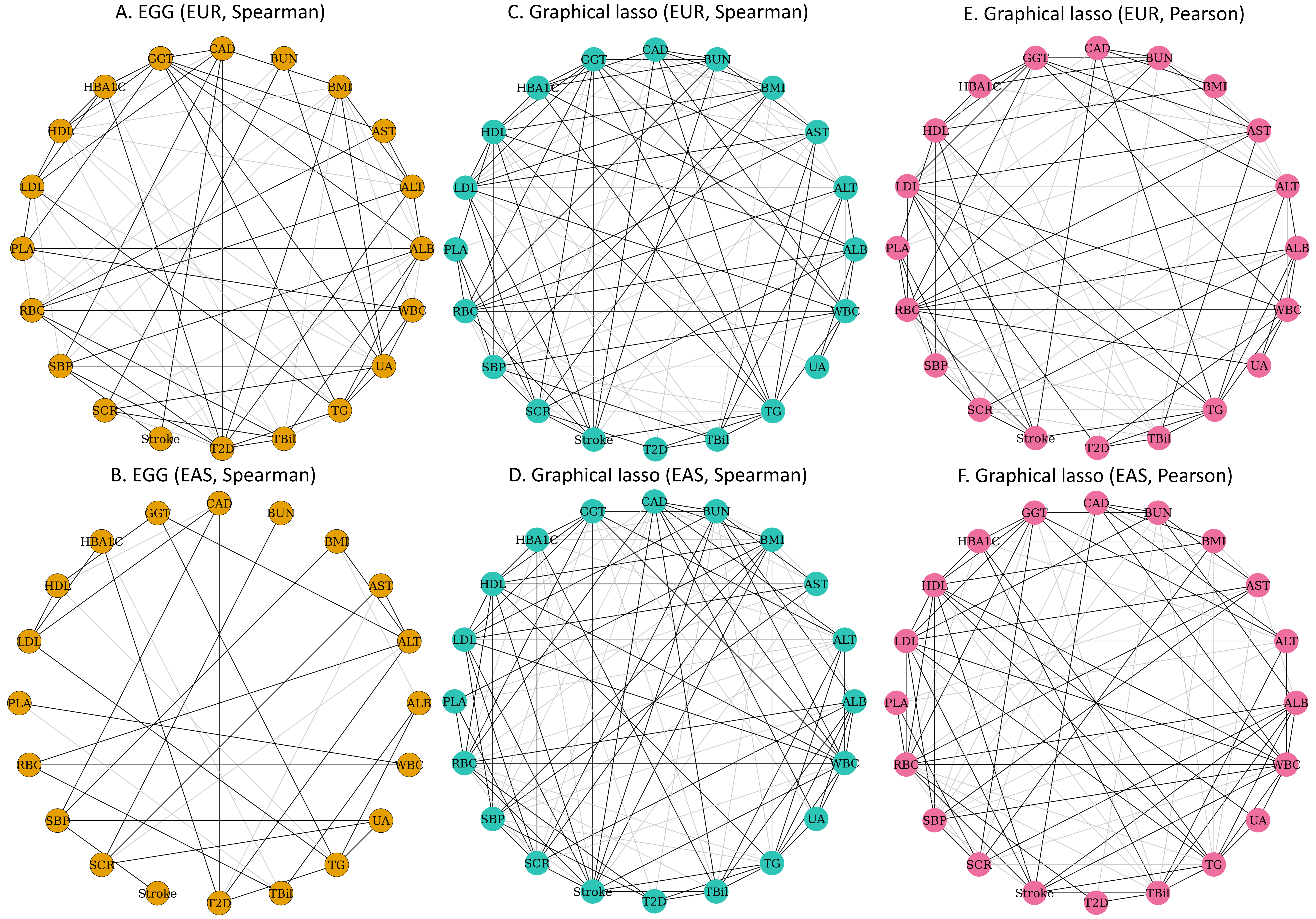
Figure 1: Panels A to C illustrate the networks of 20 metabolic and cardiovascular traits for the EUR population, as determined by EGG using Spearman’s rho, graphical lasso with Spearman’s rho, and graphical lasso with Pearson’s r, respectively. Similarly, panels D to F present the equivalent networks for the EAS population. Traits within the same category are color-coded uniformly; for instance, PLT, RBC, and WBC are all depicted in orange. In these networks, a grey edge represents a negative conditional correlation between traits, while a black edge denotes a positive conditional correlation.

We employ the EGG approach to explore the genetic network of 20 metabolic and cardiovascular traits, including CAD, T2D, stroke, body mass index (BMI), liver function markers such as alanine aminotransferase (ALT), aspartate aminotransferase (AST), $\gamma$-glutamyl transferase (GGT), and total bilirubin (TBil), blood sugar metrics glycated hemoglobin (HBA1C), kidney function indicators including serum albumin (ALB), blood urea nitrogen (BUN), serum creatinine (sCr), and uric acid (UA), blood cell counts such as platelet (PLT), red blood cell (RBC), and white blood cell (WBC) counts, serum lipids high-density lipoprotein (HDL), low-density lipoprotein (LDL), and triglycerides (TG), and systolic blood pressure (SBP). Our aim is to identify the robust genetic networks of these traits and to investigate the network difference in EUR and EAS populations. We do not include other highly correlated traits such as blood glucose, diastolic blood pressure, and pulse pressure because inclusion of highly correlated traits results in instability of network estimation. Table 1 provides a summary of the GWAS data utilized in this analysis, representing the largest GWAS sample sizes available to date for the most of traits.

We utilized the LD reference panel from the 1000 genomes project, which includes 2,490 participants and 1.67M variants in common with either HapMap3 (Consortium, 2010) or the UK Biobank (Sudlow et al., 2015). We constructed population-specific reference panels using EUR and EAS participants, each with a sample size of around 500. After allele harmonization, we obtained 1.37M variants for the EUR and 1.13M for the EAS. We then focused on variants from the union set and used the non-significant SNPs (i.e., P-value $>0.05$ for all traits) to estimate the correlation matrix $\widehat{\mathbf{R}}_{\bm{\omega}}$. This matrix was subsequently used as the correlation matrix of effect sizes in a joint $\chi^{2}_{20}$ test. Independent variants were selected from these variants survived after C+T pruning using the $\chi^{2}_{20}$ test p-values, which yield 5,458 independent variants for EUR and 2,732 independent variants for EAS, with the P-value thresholds 5E-8 and 5E-6, respectively. We adjusted the threshold for the EAS traits downward slightly due to their significantly smaller sample sizes compared to the EUR ones. These independent variants had evidence of association with at least one of the 20 traits and were not in LD. Furthermore, we employed Spearman’s rho and MAD to estimate the covariance matrix of the Z-scores and then yielded the genetic correlation matrix of the effect sizes. For other parameters, we refer to the recommendations in Section 3.4.

4.2 Results

Fig 1A presents a genetic Gaussian graph detailing the relationships among 20 metabolic and cardiovascular traits in EUR population. We observed that multiple traits, including BMI, T2D, liver function measure GGT, and lipid levels HDL and LDL, as well as SBP and Stroke, exhibited a direct connection to CAD. Notably, our study suggests the potential direct causal link between liver function and CAD conditional on other traits we included. Besides, the network also revealed a cluster of traits directly linked to T2D, including ALT, BMI, GGT, HBA1C HDL, RBC, TBil, and TG. While certain liver, kidney, and blood cell traits appear to be direct risk factors for T2D, they may not directly influence CAD. As a consequence, the previously observed causal links from RBC and HBA1C to CAD can be explained as the mediation through T2D (Wang et al., 2022). This underlines the critical role of T2D in the development of CAD, potentially mediating the impact of various metabolic traits (Ahmad et al., 2015). Furthermore, it indicated a connection between ischemic stroke and CAD, with SBP emerging as a common risk factor for both conditions. The data analysis also observed a potential protective role of higher ALB levels against ischemic stroke risk. Experimental evidence, including studies using a rat model of transient focal cerebral ischemia, suggests that ALB can prevent stroke (Cole et al., 1990). This protective effect is attributed to hemodilution caused by ALB, leading to decreased hematocrit, reduced infarct volume, and less cerebral edema.

Interestingly, We observed a negative link between BMI and SBP, which seems inconsistent with what we understand. This discrepancy can arise from the inclusion of BMI as a covariate in the blood pressure GWAS. Ideally, the genetic correlation between SBP and BMI should be zero when BMI is adjusted in SBP GWAS. However, our EGG analysis considered multiple traits simultaneously. The connection between BMI and SBP can be viewed as an association after adjusting for the rest variables that are correlated with BMI. Therefore, a negative connection can happen. We suggest that it is more reasonable to construct a network based on the GWAS summary statistics that are calculated without adjusting for any traits that are also included in the network analysis. For example, we should use SBP GWAS summary statistics without adjusting for BMI. However, in SBP GWAS, it is common to perform GWAS by adjusting for BMI.

Fig 1B presents the network in the EAS population using the same set of traits as the EUR population. Consistent with the European network, CAD was directly connected with T2D, HDL, LDL, and SBP. As for T2D, only ALT, AST, HBA1C, and TG showed direct associations. CAD and stroke were associated through their common risk factor SBP, and the protective effect of ALB for stroke was not observed in EAS. We attribute part of the difference between EUR and EAS networks to the smaller sample sizes and less statistical power in the EAS GWAS than the EUR GWAS. Theorem 2 suggests that the number of independent variants $m$ governs the estimation error of network estimate. Increasing EAS GWAS sample sizes will help uncover more causal variants, improving network analysis. Interestingly, we did not observe a negative connection between BMI and SBP, which can be attributed that SBP GWAS in EAS did not adjust for BMI.

4.3 Comparison between EGG and Graphical Lasso

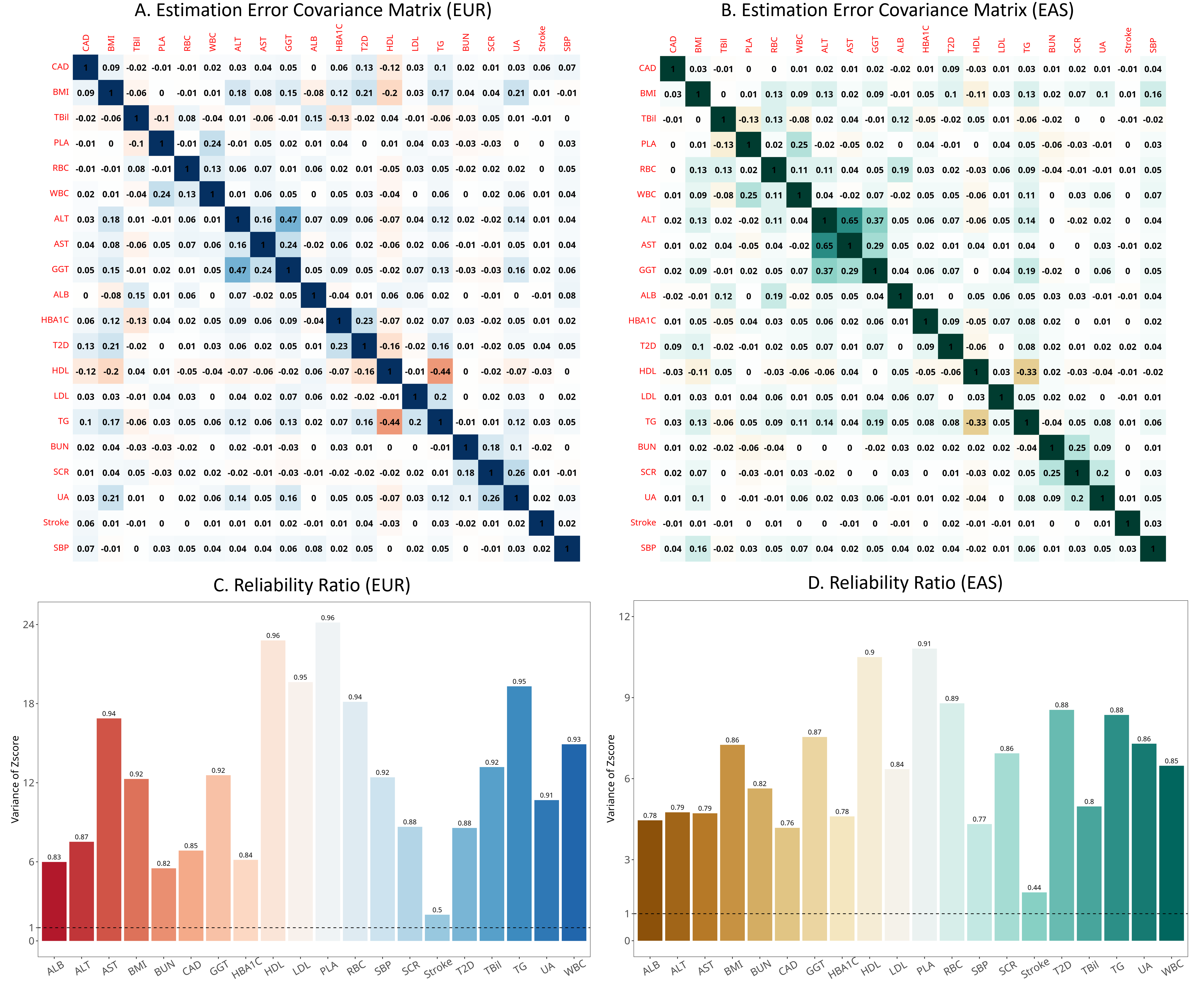
Figure 2: Panels A and B show the covariance matrix estimates of estimation errors for EUR and EAS. Panels C and D demonstrate the reliability ratio of each trait that indicates the proportion of variability in the GWAS effect estimates attributable to the true genetic effect.

To show the practical significance of EGG, we compared it with the graphical lasso (Friedman et al., 2008) with $\mathbf{\Sigma}_{\bm{\beta}}^{\texttt{Spearman}}$ and $\mathbf{\Sigma}_{\bm{\beta}}^{\texttt{Pearson}}$ as inputs. To ensure fairness, both EGG and graphical lasso were subjected to stability selection to choose the optimal lambda and employed subsampling to reduce type I errors. Panels C - F in Fig 2 present the results. The analysis revealed that the graphical lasso in both EUR and EAS leads to denser networks than EGG and the corresponding interpretation is more challenged, including multiple biologically implausible edges, such as a positive risk correlation between HDL and stroke, and a negative risk correlation between LDL and CAD. The connection between T2D and CAD disappears in the networks estimated by graphical lasso.

We consider two main factors contributing to these discrepancies. First, common tuning parameter selections like CV, which aim to find the optimal parameters for the best prediction, will asymptotically lead to inconsistent model selection (Meinshausen and Bühlmann, 2006). In contrast, non-convex penalties such as the MCP have been theoretically proved to ensure consistent model selection (Fan and Li, 2001). As EGG employs MCP while graphical lasso uses lasso, the network generated by EGG tends to be more precise. Second, the graphical lasso did not adequately address the estimation error bias. This issue is evident in Fig 2A-2B. Since the primary samples for EUR and EAS were from the UK Biobank and Biobank Japan, respectively, there are considerable sample overlaps which consequently leads to significant correlations in estimation errors. Fig 2C-2D, which demonstrate the reliability ratio of the GWAS summary data, further support this point. This ratio, calculated as $\sum_{j=1}^{m}(\hat{z}_{jk}^{2}-1)/\sum_{j=1}^{m}\hat{z}_{jk}^{2}$, reflects the proportion of variance due to genetic effects versus estimation errors (Yi, 2017). For EUR and EAS, our results indicate that genetic effects may contribute to only about 90% and 80% of the total variance of the Z-scores used to explore the networks, respectively, highlighting the significance of estimation errors. Therefore, EGG is likely to yield more interpretable genetic network estimates than graphical lasso by effectively accounting for the estimation error bias.

5 Simulation

5.1 Simulation Settings

Figure 3: Panel A displays the true genetic precision matrix with an AR(1) structure. Panel B presents the corresponding genetic correlation matrix with the AR(1) structure. Panel C illustrates the sample overlapping fractions among 20 traits. Panels D and E exhibit the counterparts of Panels A and B but follow an AR(3) structure. Panel F demonstrates the correlation matrix of estimation errors.

We consider two structures of the genetic precision matrix $\mathbf{\Theta}_{\bm{\beta}}$: AR(1) structure and AR(3) structure, and the sample overlap matrix $\mathbf{R}_{\texttt{overlap}}$ is given by $\mathbf{N}^{\texttt{overlap}}$ is of a kronecker structure. The dimension of $\widehat{\mathbf{\Theta}}_{\bm{\beta}}$ is $p=20$ which is consistent with the real data. The direct estimate of genetic covariance matrix $\texttt{cov}(\hat{\bm{\beta}}_{j})=\texttt{cov}(\bm{\beta}_{j})+\texttt{cov}(\bm{\omega}_{j})$, where the covariance of estimation error is approximately $\texttt{cov}(\omega_{jk},\omega_{js})=\texttt{cov}(X_{ik},X_{is})\times n_{jk}/\surd(n_{j}n_{k})$, where $n_{jk}/\surd(n_{j}n_{k})$ is defined as overlapping fraction. Here, we consider $\texttt{cov}(X_{ik},X_{is})=0.5$ for all traits. Fig 3 shows the structures of involved matrices.

In our study, we examined two scenarios: one with no pleiotropy and another with 10% pleiotropy. For the latter, we followed existing literature to introduce a mean shift five times the effect size for a randomly selected 10% of the independent variants (Avella-Medina et al., 2018). We employed both Pearson’s r method and Spearman’s rho method to estimate $\widehat{\mathbf{\Sigma}}_{\bm{\beta}}$, where Pearson’s method would perform poorly in the presence of pleiotropy. We considered three different sample sizes $n=$50K, 200K, 800K for all traits and three different numbers of independent variants $m=500$, 1000, 2000, which collectively explained 20% of the heritability in each trait. We use the entropy loss function $\texttt{entropy}(\mathbf{\Sigma}_{\bm{\beta}},\widehat{\mathbf{\Theta}}_{\bm{\beta}})$ and the quadratic loss function

$$\texttt{Quadratic}(\mathbf{\Sigma}_{\bm{\beta}},\widehat{\mathbf{\Theta}}_{\bm{\beta}})=\texttt{tr}\{(\mathbf{\Sigma}_{\bm{\beta}}\widehat{\mathbf{\Theta}}_{\bm{\beta}}-\mathbf{I})^{\top}(\mathbf{\Sigma}_{\bm{\beta}}\widehat{\mathbf{\Theta}}_{\bm{\beta}}-\mathbf{I})\}$$

to assess the estimation error, where $\mathbf{\Sigma}_{\bm{\beta}}$ is the true genetic correlation matrix and $\widehat{\mathbf{\Theta}}_{\bm{\beta}}$ is the related genetic precision matrix estimate. We additionally considered the following ratios:

$$t_{1}=\frac{\#\{(k,s),\ \hat{\Theta}_{\beta_{k}\beta_{s}}\neq 0,\ (k,s)\not\in\mathcal{E}\}}{p^{2}},\quad t_{2}=\frac{\#\{(k,s),\ \hat{\Theta}_{\beta_{k}\beta_{s}}=0,\ (k,s)\in\mathcal{E}\}}{p^{2}},$$ (32)

where $t_{1}$ represents the proportion of false positive edges to the total number of elements in the matrix, while $t_{2}$ represents the proportion of false negative edges to the total number of elements in the matrix. These can serve as measures for the Type-I and Type-II error rates, respectively. We compare EGG with the graphical lasso (Glasso) (Friedman et al., 2008), the constrained $\ell_{1}$-minimization for inverse matrix estimation (CLIME) (Cai et al., 2011), and penalized D-trace estimation (DLasso) (Zhang and Zou, 2014). We employed stability selection of the tuning parameters for EGG, contrasting with the Bayesian information criterion (Schwarz, 1978) used in alternative approaches. The number of replications was 1000.

5.2 Results

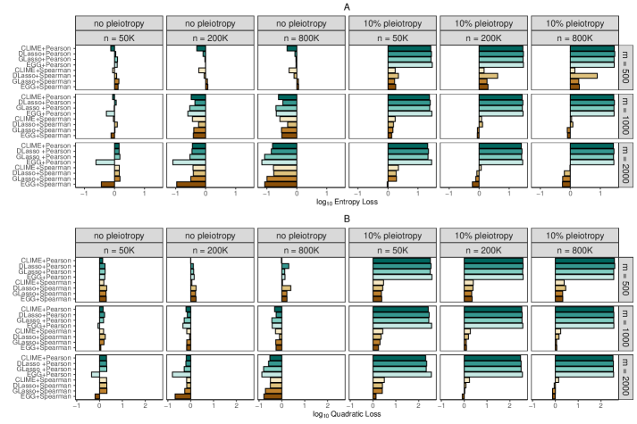
Figure 4: Panel A displays the entropy loss of the involved genetic precision matrix estimates in logarithmic scale of the AR(3) structured precision matrix. Panel B shows the corresponding quadratic loss in logarithmic scale.

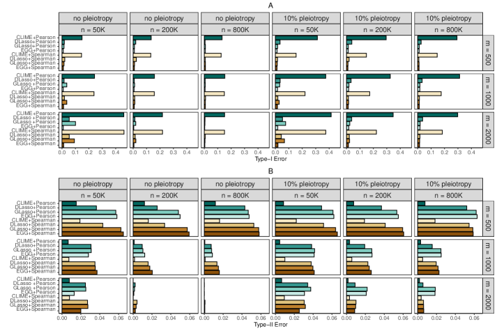
Figure 5: Panel A and B respectively displays the measures of Type-I and Type-II error rates $t_{1}$ and $t_{2}$ of the AR(3) structured precision matrix.

Fig 4 displays the bar plots of the two criteria for estimation errors: entropy loss and quadratic loss. We apply a base-10 logarithmic transformation to the estimation errors to make results more discernible. Fig 5 illustrates the bar plots for the criteria of type-I and type-II errors, denoted as $t_{1}$ and $t_{2}$. The closer the value is to 0, the more capable the network method is of replicating the true graph structure.

Fig 4 indicates that increasing $m$ has a more significant impact on reducing the network estimation error than increasing $n$. This aligns well with our theoretical expectations that the estimation error is determined by $\surd(\log n_{\texttt{eff}}/n_{\texttt{eff}})$ where $n_{\texttt{eff}}=\min(m,M,n_{1},\dots,n_{k})$. For the genetic architecture that follows a random effect model, which assumes that the genetic effects of variants approximate a normal distribution across the whole genome, increasing the GWAS sample size primarily helps us identify more causal variants, thereby improving the precision of the genetic precision matrix. In practice, independent variants passing the C+T selection can be regarded as causal variants. This means, we may need to increase the sample size such that we can identify more causal variants, making the genetic network estimated by EGG more precise.

When the model does not have pleiotropy, the EGG estimate based on $\widehat{\mathbf{\Sigma}}_{\bm{\beta}}^{\texttt{Pearson}}$ yields the smallest estimation error, slightly outperforming the EGG estimate based on $\widehat{\mathbf{\Sigma}}_{\bm{\beta}}^{\texttt{Spearman}}$. The reason is that the EGG accounts for bias caused by estimation errors, while other methods such as CLIME, GLasso, and DLasso do not. In the presence of pleiotropy, non-robust Pearson’s r-based estimates exhibited significant estimation errors, likely due to the higher sensitivity of covariance to outliers. Even in such cases, EGG still performed the best in our simulations since it corrects for biases caused by estimation errors and outliers.

The EGG consistently had the lowest Type-I error rates for identifying edges, which can be attributed to its use of stability selection. For Type-II errors, EGG performed similarly to GLasso and DLasso, suggesting that stability selection does not decrease statistical power when compared with the BIC criterion. CLIME’s lower Type-II error rate can be attributed to its higher false discovery rate. Overall, EGG maintained low levels of both types of errors, while CLIME had a higher rate of false positives.

Fig 6 and Fig 7 demonstrate the counterparts of Fig 4 and Fig 5 in the main body of our paper. In summary, their results are akin to those of the Structure AR(3) model: that is, MGG consistently performs the best under various scenarios, although the difference with existing methods isn’t substantial when there’s no pleiotropy. Under the AR(1) structure, the measures $t_{1}$ and $t_{2}$ for Type-I and Type-II error rates are both notably smaller. This can be attributed to the simpler structure of AR(1), which lacks particularly small elements, making it easier to identify true values compared to the AR(3) structure.

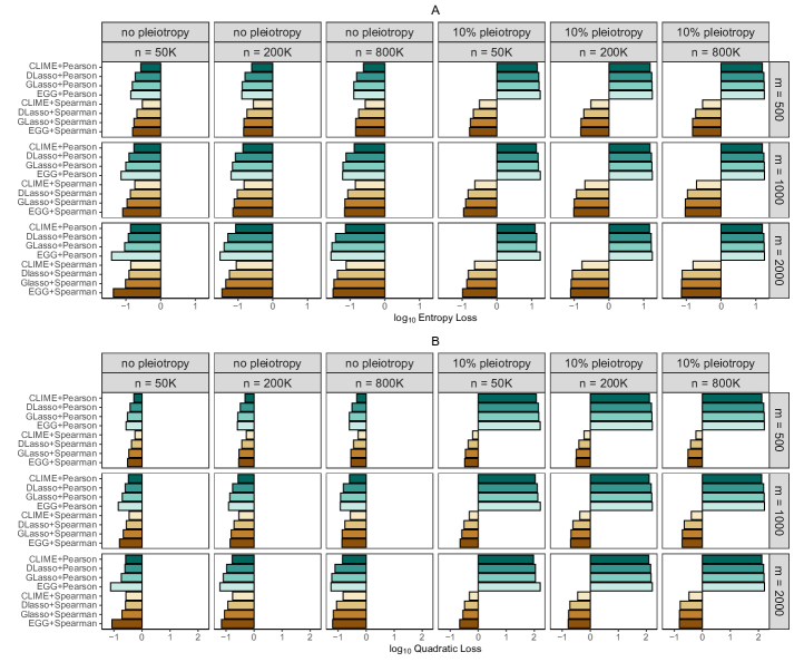
Figure 6: Panel A displays the entropy loss of the involved genetic precision matrix estimates in logarithmic scale of the AR(1) structured precision matrix. Panel B shows the corresponding quadratic loss in logarithmic scale.

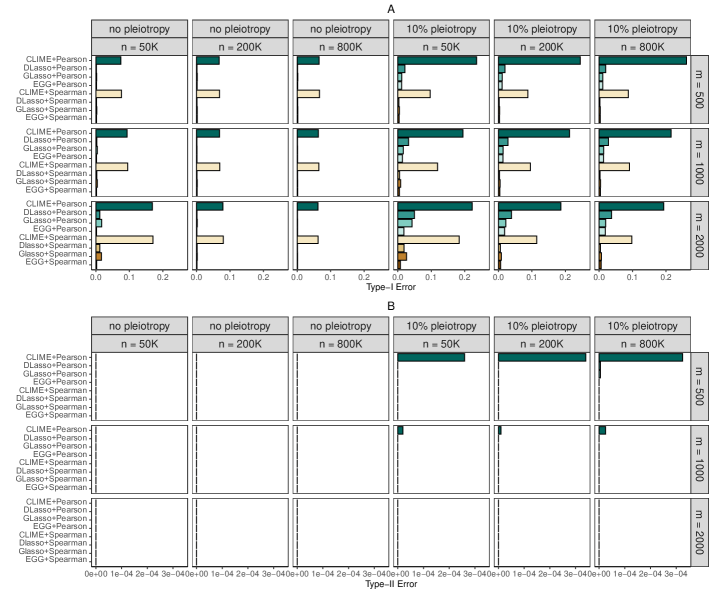
Figure 7: Panel A and B respectively displays the measures of Type-I and Type-II error rates $t_{1}$ and $t_{2}$ of the AR(1) structured precision matrix.

6 Discussion

In this paper, we present the EGG, a novel method that estimates the genetic network of multiple phenotypes by using publicly available summary statistics from GWAS. EGG is robust to the standard biases of MR including weak instruments, horizontal pleiotropy, and sample overlap by employing bias-correction for GWAS estimation error and robust genetic covariance estimation. This is the key component to make EGG superior to traditional network modeling methods. In our study, we examined Gaussian networks for 20 cardiovascular and metabolic traits, including CAD and T2D, across both EUR and EAS populations. Our findings reveal that T2D serves as a direct risk factor for CAD in both populations, underscoring the potential for synergistic treatment strategies for CAD and T2D. For both EUR and EAS, HDL acts as a direct protective factor against CAD, aligning with recent pharmaceutical trial outcomes (Group, 2017). In addition, we observe that for most metabolic traits, their influences on CAD are indirect through the mediation of blood pressure, lipids levels, and T2D. Through this real data analysis, we demonstrated that EGG represents a potentially significant advancement in both biostatistics and epidemiology, offering new insights into complex causal networks involving multiple disease traits and the related risk factors.

In biology and genetics, there are multiple definitions of phenotype network, potentially causing confusion. According to the review (Wang and Huang, 2014), three statistical networks are distinguished: marginal correlation network, partial correlation network, and Bayesian network. Marginal correlation network is undirected, based on marginal correlations between phenotypes to explore “guilt by association”, such as WGCNA used in gene co-expression analysis (Langfelder and Horvath, 2008). Partial correlation network, also undirected, derives from the partial correlation coefficient or the precision matrix, assessing phenotype independence conditional on other phenotypes. Gaussian network belongs to the class of partial correlation networks where the phenotypes are supposedly multivariate-normal distributed (Lauritzen, 1996). Indeed, GGM may be currently the most favored network approach, owing to its well-studied statistical properties and the availability of powerful tools like graphical lasso (Friedman et al., 2008) for estimation with individual-level data. The EGG method, as proposed, is novel in estimating Gaussian network from GWAS summary data, uniquely addressing estimation error bias and pleiotropy bias inherent in such data.

Bayesian network is a directed network statistically defined by a structural equation model. Currently, Bayesian network is the major technique used to represent causal diagram among phenotypes under some regularity conditions (Pearl, 2009). However, while Bayesian network holds the potential to uncover complex phenotypic relationships more effectively than partial correlation network, it suffers from substantial optimization challenges (Zheng et al., 2018), and the complexity in validating the related regularity conditions can significantly reduce the interpretability of Bayesian network estimate (Lu et al., 2023). Network deconvolution is a fourth method for network analysis, sharing the same goal of elucidating the directed network of multiple phenotypes as Bayesian network (Lin et al., 2023). However, it is not categorized among the three mainstream classes of network methods, mainly because its statistical properties have not been as thoroughly researched as those of the aforementioned methods (Pachter, 2014). Thus, directly comparing network deconvolution with GGM or Bayesian network might be premature, despite its growing popularity. Currently, no established method exists for estimating a Bayesian network of multiple phenotypes using GWAS summary data. Hence, investigating and adapting the EGG approach for this purpose represents a promising and innovative research direction. Additionally, delving into the statistical properties of network deconvolution is crucial, as it will enhance the clarity and biological interpretation of the network deconvolution estimate.

Proofs

6.1 Lemmas

In this subsection, we specify some lemmas that can facilitate the proofs, most of which can be found in the existing papers. We first discuss the equivalent characterizations of sub-Gaussian (subGau) and sub-exponential (subExp) variables.

Lemma 1 (Equivalent characterizations of sub-Guassian variables).

Given any random variable $X$, the following properties are equivalent:

• there is a constant $K_{1}\geq 0$ such that

  $$\Pr(|X|\geq t)\leq 2\exp(-t^{2}/K_{1}^{2}),\quad\text{for all }t\geq 0,$$

• the moments of $X$ satisfy

  $$||X||_{L_{p}}=(\text{E}(|X|^{p}))^{\frac{1}{p}}\leq K_{2}\surd p,\quad\text{for all }p\geq 1,$$

• the moment generating function (MGF) of $X^{2}$ satisfies:

  $$\text{E}\{\exp(\lambda^{2}X^{2})\}\leq\exp(K_{3}^{2}\lambda^{2}),\quad\text{for all $\lambda$ staisfying }|\lambda|\leq K_{3}^{-1},$$

• the MGF of $X^{2}$ is bounded at some point, namely

  $$\text{E}\{\exp(X^{2}/K_{4}^{2})\}\leq 2,$$

• if E$(X)=0$, the MGF of $X$ satisfies

  $$\text{E}\{\exp(\lambda X)\}\leq\exp(K_{5}^{2}\lambda^{2}),\quad\text{for all }\lambda\in\mathbb{R},$$

where $K_{1},\dots,K_{5}$ are certain strictly positive constants.

This lemma summarizes some well-known properties of sub-Guassian and can be found in Vershynin (2018, Proposition 2.5.2). Specifically, we call $K_{1}$ is the subGau parameter of $X$.

Lemma 2 (Equivalent characterizations of sub-exponential variables).

Given any random variable $X$, the following properties are equivalent:

• there is a constant $K_{1}\geq 0$ such that

  $$\Pr(|X|\geq t)\leq 2\exp(-t/K_{1}),\quad\text{for all }t\geq 0,$$

• the moments of $X$ satisfy

  $$||X||_{L_{p}}=(\text{E}(|X|^{p}))^{\frac{1}{p}}\leq K_{2}p,\quad\text{for all }p\geq 1,$$

• the moment generating function (MGF) of $|X|$ satisfies:

  $$\text{E}\{\exp(\lambda|X|)\}\leq\exp(K_{3}\lambda),\quad\text{for all $\lambda$ staisfying }0\leq\lambda\leq K_{3}^{-1},$$

• the MGF of $|X|$ is bounded at some point, namely

  $$\text{E}\{\exp(|X|/K_{4})\}\leq 2,$$

• if E$(X)=0$, the MGF of $X$ satisfies

  $$\text{E}\{\exp(\lambda X)\}\leq\exp(K_{5}^{2}\lambda^{2}),\quad\text{for all }\lambda\leq K_{5}^{-1},$$

where $K_{1},\dots,K_{5}$ are certain strictly positive constants.

This lemma summarizes some well-known properties of sub-exponential and can be found in Vershynin (2018, Proposition 2.7.1). Specifically, we call $K_{1}$ is the subExp parameter of $X$.

Lemma 3 (Product of sub-Gaussian variable is sub-exponential).

Suppose that $X,Z$ are two sub-Gaussian variable, then $Y=XZ$ is a sub-exponential variable. Besides, if $X$ is a bounded sub-Gaussian variable, then then $Y=XZ$ is a sub-Gaussian variable.

The first claim of this lemma is provided by Vershynin (2018, Proposition 2.7.7). The second claim is proved as follows:

$$\Pr(Y\geq t)\leq\Pr)(X\geq\bar{X})+\Pr(Z\geq(t/\bar{X}))=\Pr(Z\geq(t/\bar{X}))\leq\exp(-t^{2}/(\bar{X}^{2}K_{1}^{2})),$$ (33)

where $\bar{X}$ is the bound of $|X|$ and $K_{1}$ is the subGau parameter of $Z$. It should be pointed out that if $K_{1}$ is the subGau/subExp parameter of random variable $X$, then for any constant $K_{1}^{\prime}>K1$, $K_{1}^{\prime}$ is also the subGau/subExp parameter of $X$. The minimum subGau and subExp parameter for a random variable is defined by

$$||X||_{\psi_{2}}=\inf\{t>0:\ \texttt{E}(X^{2}/t^{2})\leq 2\}$$ (34)

$$||X||_{\psi_{1}}=\inf\{t>0:\ \texttt{E}(|X|/t)\leq 2\}.$$ (35)

See Vershynin (2018, Chapter 2) for more details.

6.2 Preliminary properties of random effect model

We deduce some basic properties of the random effect model. Recall that a multivariate variable $\bm{X}_{i}=(X_{i1},\dots,X_{ip})^{\top}$ with

$$X_{ij}=\eta_{ij}+\epsilon_{ij},$$

where $\eta_{ij}$ is a part of $X_{ij}$ determined by its genotype and $\epsilon_{ij}$ is a modifiable effect orthogonal to the genetic effect $\eta_{ij}$. The random effect model assumes

$$\eta_{ik}=\sum_{j=1}^{m}G_{ij}\beta_{jk}=\bm{G}_{i}^{\top}\bm{\beta}_{k},$$

where $\bm{G}_{i}=(G_{i1},\dots,G_{im})^{\top}$ are $m$ genetic variants, $\bm{\beta}_{k}=(\beta_{j1},\dots,\beta_{jp})^{\top}$ are $m$ genetic effects on the $k$th trait. Besides, $\bm{G}_{i}$ and $\bm{\beta}_{j}$ are considered mutually independent and follow the sub-Gaussian distributions defined in conditions (C1) and (C2). Next,

$$\texttt{cov}(\bm{X}_{i})=\mathbf{\Sigma}_{X},$$

whose diagonal elements are all 1. Finally, we set

$$\Pr(|\beta_{jk}|\geq t)=\Pr(|\sqrt{m}\beta_{jk}|\geq\sqrt{m}t)\leq 2\exp(-mt^{2}/\kappa_{\beta}^{2}),$$

$$\Pr(|\epsilon_{ik}|\geq t)\leq 2\exp(-t^{2}/\kappa_{\epsilon}^{2})$$

where $\kappa_{\beta}$ is the subGau parameter for $\sqrt{m}\beta_{jk}$, $1\leq j\leq m$, $1\leq k\leq p$, and $\kappa_{\epsilon}$ is the subGau parameter for $\epsilon_{ik}$, $1\leq i\leq n_{k}$, $1\leq k\leq p$. The bounds of $|G_{ij}|$ and $|F_{ij}|$ are $\bar{g}$ and $\bar{f}$, respectively.

We first show

$$\Pr(|G_{ij}\beta_{jk}|\geq t)\leq\Pr(|G_{ij}|\geq\bar{g})+\Pr\bigg{(}|\beta_{jk}|\geq\frac{t}{\bar{g}}\bigg{)}\leq 0+2\exp\bigg{(}-\frac{mt^{2}}{\bar{g}^{2}\kappa_{\beta}^{2}}\bigg{)},$$ (36)

which indicate that $\sqrt{m}G_{ij}\beta_{jk}$ is a subGau variable with a subGau parameter $\bar{g}\kappa_{\beta}$. Next,

$$\Pr(|\eta_{ij}|\geq t)=\Pr\bigg{(}\bigg{|}\sum_{j=1}^{m}g_{ij}\beta_{jk}\bigg{|}\geq t\bigg{)}\leq 2\exp\bigg{(}-\frac{t^{2}}{\bar{g}^{2}\kappa_{\beta}^{2}}\bigg{)},$$ (37)

$$\Pr(|\eta_{ij}-G_{ij}\beta_{jk}|\geq t)=\Pr\bigg{(}\bigg{|}\sum_{z\neq j}^{m}g_{iz}\beta_{zk}\bigg{|}\geq t\bigg{)}\leq 2\exp\bigg{(}-\frac{m}{m-1}\frac{t^{2}}{\bar{g}^{2}\kappa_{\beta}^{2}}\bigg{)}\leq 2\exp\bigg{(}-\frac{t^{2}}{\bar{g}^{2}\kappa_{\beta}^{2}}\bigg{)},$$ (38)

which indicates $\eta_{ij}$ and $\eta_{ij}-G_{ij}\beta_{jk}$ are two subGau variables with subGau parameter $\bar{g}\kappa_{\beta}$. Next,

$$\Pr(|X_{ik}|\geq t)=\Pr(|\eta_{ik}+\epsilon_{ik}|\geq t)\leq 2\exp\bigg{(}-\frac{t^{2}}{C_{x}\bar{g}^{2}\kappa_{\beta}^{2}+C_{x}\kappa_{\epsilon}^{2}}\bigg{)},$$ (39)

$$\Pr(|X_{ik}-G_{ij}\beta_{jk}|\geq t)=\Pr(|\eta_{ik}-G_{ij}\beta_{jk}+\epsilon_{ik}|\geq t)\leq 2\exp\bigg{(}-\frac{t^{2}}{C_{x}\bar{g}^{2}\kappa_{\beta}^{2}+C_{x}\kappa_{\epsilon}^{2}}\bigg{)},$$ (40)

where $C_{x}\geq 0$ is a constant, which indicates $x_{ij}$ and $x_{ij}-G_{ij}\beta_{jk}$ are two subGau variables with subGau parameter $\sqrt{C_{x}(\bar{g}^{2}\kappa_{\beta}^{2}+\kappa_{\epsilon}^{2})}$.

6.3 Convergence Rate of $\hat{\mathbf{\Sigma}}_{\omega_{k}\omega_{s}}$

We derive the covergence rate of the estimate of the estimation error covariance matrix $\hat{\mathbf{\Sigma}}_{\bm{\omega}}$. Recall that

$$\hat{b}_{jk}=\frac{1}{n_{k}}\sum_{i=1}^{n_{k}}F_{ij}X_{ik}.$$ (41)

We first investigate that

$$\Pr(|F_{ij}X_{ik}|\geq t)\leq\Pr(|F_{ij}|\geq\bar{f})+\Pr\bigg{(}|X_{ik}|\geq\frac{t}{\bar{f}}\bigg{)}\leq 2\exp\bigg{(}-\frac{t^{2}}{C_{x}\bar{f}^{2}\bar{g}^{2}\kappa_{\beta}^{2}+C_{x}\bar{f}^{2}\kappa_{\epsilon}^{2}}\bigg{)}.$$ (42)

Hence, $\hat{b}_{jk}$ is a subGau variable with subGau parameter $C_{x}\bar{f}\sqrt{\bar{g}^{2}\kappa_{\beta}^{2}+\kappa_{\epsilon}^{2}}$, and $\hat{b}_{jk}\hat{b}_{js}$ is a subExp variable with subExp parameter $C_{x}^{2}\bar{f}^{2}(\bar{g}^{2}\kappa_{\beta}^{2}+\kappa_{\epsilon}^{2})$. By using Theorem 9.3 in fa,

$$\Pr\bigg{(}\bigg{|}\frac{1}{M}\sum_{j=1}^{M}(\hat{b}_{jk}\hat{b}_{js}-\texttt{E}(\hat{b}_{jk}\hat{b}_{js}))\bigg{|}\geq\frac{2t}{\texttt{var}(\hat{b}_{jk})\texttt{var}(\hat{b}_{js})}\bigg{)}\leq 2\exp(-c_{M}Mt^{2}),$$ (43)

where $c_{M}$ is a constant and $t\leq\sqrt{M}/2$.

The next step is showing what $\texttt{var}(\hat{b}_{jk})$, $\texttt{var}(\hat{b}_{js})$, and $\texttt{E}(\hat{b}_{jk}\hat{b}_{js}))$ are. Specifically,

$$\texttt{var}(\hat{b}_{jk})=\texttt{var}\bigg{(}\frac{1}{n_{k}}\sum_{i=1}^{n_{k}}F_{ij}X_{ik}\bigg{)}=\frac{1}{n_{k}^{2}}\texttt{var}(X_{ik})\texttt{var}(F_{ij})=\frac{1}{n_{k}^{2}},$$ (44)

since $\texttt{var}(X_{ik})=\texttt{var}(F_{ij})=1$. As for $\texttt{E}(\hat{b}_{jk}\hat{b}_{js}))$,

$$\texttt{E}(\hat{b}_{jk}\hat{b}_{ls})) =\texttt{E}\bigg{\{}\bigg{(}\frac{1}{n_{k}}\sum_{i=1}^{n_{k}}F_{ij}X_{ik}\bigg{)}\bigg{(}\frac{1}{n_{k}}\sum_{i=1}^{n_{s}}F_{ij}X_{is}\bigg{)}\bigg{\}}=\texttt{E}\bigg{(}\frac{1}{n_{k}n_{s}}\sum_{i=1}^{n_{k}}\sum_{t=1}^{n_{s}}F_{ij}X_{ik}F_{tj}X_{ts}\bigg{)}$$

$$=\texttt{E}\bigg{[}\texttt{E}\bigg{(}\frac{1}{n_{k}n_{s}}\sum_{i=1}^{n_{k}}\sum_{t=1}^{n_{s}}F_{ij}F_{tj}\bigg{|}X_{ik}X_{ts}\bigg{)}\bigg{]}=\texttt{E}\bigg{(}\frac{1}{n_{k}n_{s}}\sum_{i=1}^{n_{k}}\sum_{t=1}^{n_{s}}X_{ik}X_{ts}\bigg{)}$$

$$=\texttt{E}\bigg{(}\frac{1}{n_{k}n_{s}}\sum_{i\in\mathcal{O}_{ks}}X_{ik}X_{is}\bigg{)}=\frac{n_{ks}\texttt{cov}(X_{ik},X_{is})}{n_{k}n_{s}},$$ (45)

where $\mathcal{O}_{ks}$ is the set of overlapping samples in the $k$th and $s$th GWAS cohorts. This consistent with the results in our previous work Lorincz-Comi et al. (2023).

6.4 Convergence rate of $\hat{\Sigma}_{\beta_{k}\beta_{s}}$

Then, we investigate the sub-Gaussianity of the GWAS estimates. First,

$$\hat{\beta}_{jk}-\beta_{jk} =\frac{1}{n_{k}}\sum_{i=1}^{n_{k}}(G_{ij}^{2}-1)\beta_{jk}+\frac{1}{n_{k}}\sum_{i=1}^{n_{k}}G_{ij}(X_{ik}-G_{ij}\beta_{jk})$$

$$=\omega_{jk}=\omega_{1jk}+\omega_{2jk}.$$ (46)

For $\omega_{1jk}$, we first note that $(G_{ij}^{2}-1)$ is a subGau variable bounded by $\bar{g}^{2}+1+2\bar{g}$. Hence,

$$\Pr(|(G_{ij}^{2}-1)\beta_{jk}|\geq t)\leq\Pr\bigg{(}|\beta_{jk}|\geq\frac{t}{\bar{g}^{2}+1+2\bar{g}}\bigg{)}\leq 2\exp\bigg{(}-\frac{mt^{2}}{2\kappa_{\beta}^{2}(\bar{g}^{2}+1+2\bar{g})^{2}}\bigg{)},$$ (47)

and

$$\Pr(|\omega_{1jk}|\geq t)=\Pr\bigg{(}\bigg{|}\sum_{i=1}^{n_{k}}(G_{ij}^{2}-1)\beta_{jk}\bigg{|}\geq n_{k}t\bigg{)}\leq 2\exp\bigg{(}-\frac{n_{k}mt^{2}}{2\kappa_{\beta}^{2}(\bar{g}^{2}+1+2\bar{g})^{2}}\bigg{)},$$ (48)

which indicates that $\omega_{1jk}$ is a subGau variable with a subGau parameter $\sqrt{\frac{C_{x}}{n_{k}m}\kappa_{\beta}(\bar{g}^{2}+1+2\bar{g})}$. The estimation error $\omega_{2jk}$ satisfies:

$$\Pr(|\omega_{2jk}|\geq t)=\Pr\bigg{(}\bigg{|}\sum_{i=1}^{n_{k}}G_{ij}(X_{ik}-G_{ij}\beta_{jk})\bigg{|}\geq n_{k}t\bigg{)} \leq\Pr(|G_{ij}|\geq\bar{g})+\Pr\bigg{(}\bigg{|}\sum_{i=1}^{n_{k}}X_{ik}-G_{ij}\beta_{jk}\bigg{|}\geq\frac{n_{k}t}{\bar{g}}\bigg{)}$$

$$\leq 2\exp\bigg{(}-\frac{n_{k}t^{2}}{C_{x}\bar{g}^{4}\kappa_{\beta}^{2}+C_{x}\kappa_{\epsilon}^{2}\bar{g}^{2}}\bigg{)},$$ (49)

which indicates that $\omega_{2jk}$ is a subGau variable with a subGau parameter $\sqrt{\frac{C_{x}}{n_{k}}(\bar{g}^{4}\kappa_{\beta}^{2}+\kappa_{\epsilon}^{2}\bar{g}^{2})}$. Note that the subGau parameter of $\omega_{1jk}$ is smaller than $\omega_{2jk}$ when

$$m\geq\frac{\kappa_{\beta}^{2}(\bar{g}^{2}+1+2\bar{g})^{2}}{\bar{g}^{4}\kappa_{\beta}^{2}+\kappa_{\epsilon}^{2}\bar{g}^{2}}.$$ (50)

Hence, we can consider $\omega_{jk}=\omega_{1jk}+\omega_{2jk}$ is a subGau variable with subGau parameter $\sqrt{\frac{2C_{x}}{n_{k}}(\bar{g}^{4}\kappa_{\beta}^{2}+\kappa_{\epsilon}^{2}\bar{g}^{2})}$ if (50) holds.

We consider

$$\frac{1}{m}\sum_{j=1}^{m}\hat{\beta}_{jk}\hat{\beta}_{js}=\frac{1}{m}\sum_{j=1}^{m}(\beta_{jk}+\omega_{jk})(\beta_{js}+\omega_{js})=\frac{1}{m}\sum_{j=1}^{m}(\beta_{jk}\beta_{js}+\omega_{jk}\beta_{js}+\omega_{js}\beta_{jk}+\omega_{jk}\omega_{js}),$$ (51)

and hence

$$\frac{1}{m}\sum_{j=1}^{m}(\hat{\beta}_{jk}\hat{\beta}_{js}-\Sigma_{w_{k}w_{s}}-\Sigma_{\beta_{k}\beta_{s}})=I_{1}+I_{2}+I_{3}+I_{4},$$ (52)

where

$$I_{1}=\frac{1}{m}\sum_{j=1}^{m}(\beta_{jk}\beta_{js}-\Sigma_{\beta_{k}\beta_{s}}),~{}I_{2}=\frac{1}{m}\sum_{j=1}^{m}(\omega_{jk}\omega_{js}-\Sigma_{\omega_{k}\omega_{s}}),~{}I_{3}=\frac{1}{m}\sum_{j=1}^{m}\omega_{jk}\beta_{js},~{}I_{4}=\frac{1}{m}\sum_{j=1}^{m}\omega_{js}\beta_{jk}.$$

As for $I_{1}$, $\beta_{jk}\beta_{js}$ is a subExp. variable with a subExp. parameter $\frac{1}{m}\kappa_{\beta}^{2}$ that leads to

$$\Pr(|I_{1}|\geq t\sqrt{\Sigma_{\beta_{k}\beta_{k}}\Sigma_{\beta_{s}\beta_{s}}})\leq 2\exp\bigg{\{}-mC_{\beta\beta}\min\bigg{(}\frac{m^{2}t^{2}\Sigma_{\beta_{k}\beta_{k}}\Sigma_{\beta_{s}\beta_{s}}}{\kappa_{\beta}^{4}},\frac{mt\sqrt{\Sigma_{\beta_{k}\beta_{k}}\Sigma_{\beta_{s}\beta_{s}}}}{\kappa_{\beta}^{2}}\bigg{)}\bigg{\}},$$ (53)

where $C_{\beta\beta}$ is a constant.

As for $I_{2}$, $\omega_{jk}\omega_{js}$ is a subExp. variable with a subExp. parameter $\frac{C_{I_{2}}}{\sqrt{n_{k}n_{s}}}$ that leads to

$$\Pr(|I_{2}|\geq t\sqrt{\Sigma_{\beta_{k}\beta_{k}}\Sigma_{\beta_{s}\beta_{s}}})\leq 2\exp\bigg{\{}-mC_{\omega\omega}\min\bigg{(}\frac{t^{2}n_{k}n_{s}\Sigma_{\beta_{k}\beta_{k}}\Sigma_{\beta_{s}\beta_{s}}}{C_{I_{2}}^{2}},\frac{t\sqrt{n_{k}n_{s}\Sigma_{\beta_{k}\beta_{k}}\Sigma_{\beta_{s}\beta_{s}}}}{C_{I_{2}}}\bigg{)}\bigg{\}},$$ (54)

where $C_{I_{2}}=2C_{x}(\bar{g}^{4}\kappa_{\beta}^{2}+\kappa_{\epsilon}^{2}\bar{g}^{2})$ and $C_{\omega\omega}$ is a constant.

As for $I_{3}$, $\omega_{jk}\beta_{js}$ is a subExp. variable with a subExp. parameter $\frac{C_{I3}}{\sqrt{n_{k}m}}$ that leads to

$$\Pr(|I_{3}|\geq t\sqrt{\Sigma_{\beta_{k}\beta_{k}}\Sigma_{\beta_{s}\beta_{s}}})\leq 2\exp\bigg{\{}-mC_{\beta\omega}\min\bigg{(}\frac{t^{2}n_{k}m\Sigma_{\beta_{k}\beta_{k}}\Sigma_{\beta_{s}\beta_{s}}}{C_{I_{3}}^{2}},\frac{t\sqrt{mn_{k}\Sigma_{\beta_{k}\beta_{k}}\Sigma_{\beta_{s}\beta_{s}}}}{C_{I_{3}}}\bigg{)}\bigg{\}},$$ (55)

where $C_{I_{3}}=2C_{x}(\bar{g}^{4}\kappa_{\beta}^{4}+\kappa_{\epsilon}^{2}\bar{g}^{2}\kappa_{\beta}^{2})^{\frac{1}{2}}$ and $C_{\beta\omega}$ is a constant.

As for $I_{4}$, it is easy to obtain

$$\Pr(|I_{4}|\geq t\sqrt{\Sigma_{\beta_{k}\beta_{k}}\Sigma_{\beta_{s}\beta_{s}}})\leq 2\exp\bigg{\{}-mC_{\beta\omega}\min\bigg{(}\frac{t^{2}n_{s}m\Sigma_{\beta_{k}\beta_{k}}\Sigma_{\beta_{s}\beta_{s}}}{C_{I_{3}}^{2}},\frac{t\sqrt{mn_{s}\Sigma_{\beta_{k}\beta_{k}}\Sigma_{\beta_{s}\beta_{s}}}}{C_{I_{3}}}\bigg{)}\bigg{\}},$$ (56)

since it is essentially a duplicate of $I_{3}$. Note that

$$\Pr\bigg{\{}\bigg{|}\frac{1}{m}\sum_{j=1}^{m}(\hat{\beta}_{jk}\hat{\beta}_{js}-\Sigma_{w_{k}w_{s}}-\Sigma_{\beta_{k}\beta_{s}})\bigg{|}\geq t\bigg{\}}\leq\sum_{l=1}^{4}\Pr(|I_{l}|\geq t),$$ (57)

and

$$\Sigma_{\beta_{k}\beta_{k}}\Sigma_{\beta_{s}\beta_{s}}=\frac{h^{2}_{k}h^{2}_{s}}{m^{2}},$$ (58)

$h^{2}_{k}$, $h^{2}_{s}$ are two constants. On the other, we apply a universal constant $\bar{C}$ to replace all constant in (53-56) and apply the minimum sample size $n_{\textsf{min}}$ to replace the sample size $n_{k}$, $n_{s}$, which results in

$$\Pr(|I_{1}|\geq t\sqrt{\Sigma_{\beta_{k}\beta_{k}}\Sigma_{\beta_{s}\beta_{s}}})\leq 2\exp\bigg{(}-\bar{C}\min(t^{2}m,tm)\bigg{)},$$ (59)

$$\Pr(|I_{2}|\geq t\sqrt{\Sigma_{\beta_{k}\beta_{k}}\Sigma_{\beta_{s}\beta_{s}}})\leq 2\exp\bigg{(}-\bar{C}\min(t^{2}n_{\textsf{min}}^{2}m^{-1},tn_{\textsf{min}})\bigg{)},$$ (60)

$$\Pr(|I_{3}|\geq t\sqrt{\Sigma_{\beta_{k}\beta_{k}}\Sigma_{\beta_{s}\beta_{s}}})= \Pr(|I_{4}|\geq t\sqrt{\Sigma_{\beta_{k}\beta_{k}}\Sigma_{\beta_{s}\beta_{s}}})\leq 2\exp\bigg{(}-\bar{C}\min(t^{2}n_{\textsf{min}}m,t\sqrt{n_{\textsf{min}}m})\bigg{)}.$$ (61)

Hence, by letting

$$n_{\text{eff}}=\min\{m,M,n_{1},\dots,n_{p}\},$$ (62)

we prove that for any $t\leq 1$,

$$\Pr\bigg{\{}\bigg{|}\frac{1}{m}\sum_{j=1}^{m}\bigg{(}\hat{\beta}_{jk}\hat{\beta}_{js}-\Sigma_{w_{k}w_{s}}-\Sigma_{\beta_{k}\beta_{s}}\bigg{)}\bigg{|}\geq t\sqrt{\Sigma_{\beta_{k}\beta_{k}}\Sigma_{\beta_{s}\beta_{s}}}\bigg{\}}\leq 8\exp(-\bar{C}n_{\text{eff}}t^{2}).$$ (63)

After proving this central concentration inequality, we then to prove $\hat{\mathbf{\Sigma}}_{\bm{\beta}}^{\texttt{Pearson}}$ and $\hat{\mathbf{\Sigma}}_{\bm{\beta}}^{\texttt{Spearman}}$. For $\hat{\mathbf{\Sigma}}_{\bm{\beta}}^{\texttt{Pearson}}$,

$$\hat{\Sigma}_{\beta_{k}\beta_{s}}^{\texttt{Pearson}}-\Sigma_{\beta_{k}\beta_{s}}=\frac{1}{m}\sum_{j=1}^{m}(\hat{\beta}_{jk}\hat{\beta}_{js}-\Sigma_{w_{k}w_{s}}-\Sigma_{\beta_{k}\beta_{s}})+\Sigma_{w_{k}w_{s}}-\hat{\Sigma}_{w_{k}w_{s}}.$$ (64)

Hence,

$$\Pr(|\hat{\Sigma}_{\beta_{k}\beta_{s}}^{\texttt{Pearson}}-\Sigma_{\beta_{k}\beta_{s}}|\geq t\sqrt{\Sigma_{\beta_{k}\beta_{k}}\Sigma_{\beta_{s}\beta_{s}}}) \leq\Pr\bigg{\{}\bigg{|}\frac{1}{m}\sum_{j=1}^{m}\bigg{(}\hat{\beta}_{jk}\hat{\beta}_{js}-\Sigma_{w_{k}w_{s}}-\Sigma_{\beta_{k}\beta_{s}}\bigg{)}\bigg{|}\geq t\sqrt{\Sigma_{\beta_{k}\beta_{k}}\Sigma_{\beta_{s}\beta_{s}}}\bigg{)}$$

$$+\Pr\bigg{(}|\Sigma_{w_{k}w_{s}}-\hat{\Sigma}_{w_{k}w_{s}}|\geq t\sqrt{\Sigma_{\beta_{k}\beta_{k}}\Sigma_{\beta_{s}\beta_{s}}}\bigg{)}$$

$$\leq 10\exp(-\bar{C}n_{\textsf{eff}}t^{2}),$$ (65)

for any $t\leq 1$.

As for $\hat{\mathbf{\Sigma}}_{\bm{\beta}}^{\texttt{Spearman}}$, it has the same formula of central concentration inequality as $\hat{\mathbf{\Sigma}}_{\bm{\beta}}^{\texttt{Pearson}}$:

$$\Pr(|\hat{\Sigma}_{\beta_{k}\beta_{s}}^{\texttt{Spearman}}-\Sigma_{\beta_{k}\beta_{s}}|\geq t\sqrt{\Sigma_{\beta_{k}\beta_{k}}\Sigma_{\beta_{s}\beta_{s}}})\leq C^{\prime}\exp(-\bar{C}^{\prime}n_{\textsf{eff}}t^{2}),$$ (66)

where $C^{\prime},\bar{C}^{\prime}$ is are two constants. Since $\hat{\beta}_{jk}=\beta_{jk}+\omega_{jk}$ is the sum of two subGau variable (and hence is also a subGau variable), we use the results of Avella-Medina et al. (2018) to prove that

$$\Pr\bigg{(}|\hat{D}_{\beta_{s}}\hat{D}_{\beta_{k}}\hat{R}_{\beta_{s}\beta_{k}}-\texttt{se}(\hat{\beta}_{js})\texttt{cor}(\hat{\beta}_{jk}\hat{\beta}_{js})\texttt{se}(\hat{\beta}_{js})|\geq t\texttt{se}(\hat{\beta}_{jk})\texttt{se}(\hat{\beta}_{js})\bigg{)}\leq C_{1}\exp(-C_{2}mt^{2}),$$ (67)

where

$$\texttt{se}(\hat{\beta}_{jk})=\Sigma_{\beta_{k}\beta_{k}}+\Sigma_{\omega_{k}\omega_{k}},\quad\texttt{cor}(\hat{\beta}_{jk}\hat{\beta}_{js})=\frac{\Sigma_{\beta_{k}\beta_{s}}+\Sigma_{\omega_{k}\omega_{s}}}{\sqrt{\Sigma_{\beta_{k}\beta_{k}}+\Sigma_{\omega_{k}\omega_{k}}}\sqrt{\Sigma_{\beta_{s}\beta_{s}}+\Sigma_{\omega_{s}\omega_{s}}}},$$

and hence

$$\texttt{se}(\hat{\beta}_{js})\texttt{cor}(\hat{\beta}_{jk}\hat{\beta}_{js})\texttt{se}(\hat{\beta}_{js})=\Sigma_{\beta_{k}\beta_{s}}+\Sigma_{\omega_{k}\omega_{s}}.$$

and $C_{1},C_{2}$ are certain constants. Therefore,

$$\Pr(|\hat{D}_{\beta_{s}}\hat{D}_{\beta_{k}}\hat{R}_{\beta_{s}\beta_{k}} -\Sigma_{\beta_{k}\beta_{s}}-\Sigma_{\omega_{k}\omega_{s}}+\Sigma_{\omega_{k}\omega_{s}}-\hat{\Sigma}_{\omega_{k}\omega_{s}}|\geq t\sqrt{\Sigma_{\beta_{k}\beta_{k}}\Sigma_{\beta_{s}\beta_{s}}})$$

$$\leq\Pr(|\hat{D}_{\beta_{s}}\hat{D}_{\beta_{k}}\hat{R}_{\beta_{s}\beta_{k}})-\Sigma_{\beta_{k}\beta_{s}}-\Sigma_{\omega_{k}\omega_{s}}|\geq t\sqrt{\Sigma_{\beta_{k}\beta_{k}}\Sigma_{\beta_{s}\beta_{s}}})$$

$$+\Pr(|\Sigma_{\omega_{k}\omega_{s}}-\hat{\Sigma}_{\omega_{k}\omega_{s}}|\geq t\sqrt{\Sigma_{\beta_{k}\beta_{k}}\Sigma_{\beta_{s}\beta_{s}}}).$$ (68)

Here,

$$\Pr(|\hat{D}_{\beta_{s}}\hat{D}_{\beta_{k}}\hat{R}_{\beta_{s}\beta_{k}} -\Sigma_{\beta_{k}\beta_{s}}-\Sigma_{\omega_{k}\omega_{s}}|\geq t\sqrt{\Sigma_{\beta_{k}\beta_{k}}\Sigma_{\beta_{s}\beta_{s}}})$$

$$=\Pr(|\hat{D}_{\beta_{s}}\hat{D}_{\beta_{k}}\hat{R}_{\beta_{s}\beta_{k}})-\Sigma_{\beta_{k}\beta_{s}}-\Sigma_{\omega_{k}\omega_{s}}|\geq t^{\prime}\texttt{se}(\hat{\beta}_{jk})\texttt{se}(\hat{\beta}_{js})),$$ (69)

where

$$t^{\prime}=t\sqrt{\frac{\Sigma_{\beta_{k}\beta_{k}}\Sigma_{\beta_{s}\beta_{s}}}{(\Sigma_{\beta_{k}\beta_{k}}+\Sigma_{\omega_{k}\omega_{k}})(\Sigma_{\beta_{s}\beta_{s}}+\Sigma_{\omega_{s}\omega_{s}})}}.$$

Note that $t^{\prime}<1$ because $\Sigma_{\beta_{k}\beta_{k}},\Sigma_{\omega_{k}\omega_{k}},\Sigma_{\beta_{s}\beta_{s}},\Sigma_{\omega_{s}\omega_{s}}$ are all positive numbers. Hence. by choosing $C^{\prime},\bar{C}^{\prime}$ constants properly, we prove

$$\Pr(|\hat{\Sigma}_{\beta_{k}\beta_{s}}^{\texttt{Spearman}}-\Sigma_{\beta_{k}\beta_{s}}|\geq t\sqrt{\Sigma_{\beta_{k}\beta_{k}}\Sigma_{\beta_{s}\beta_{s}}})\leq C^{\prime}\exp(-\bar{C}^{\prime}n_{\textsf{eff}}t^{2}).$$ (70)

6.5 Proof of Theorem 1

It is easy to see that

$$\Pr\bigg{\{}\max_{1\leq k\leq s\leq p}\bigg{(}|\hat{\Sigma}_{\beta_{k}\beta_{s}}^{\texttt{Pearson}}-\Sigma_{\beta_{k}\beta_{s}}|\geq t\sqrt{\Sigma_{\beta_{k}\beta_{k}}\Sigma_{\beta_{s}\beta_{s}}}\bigg{)}\bigg{\}} \leq\sum_{j=1}^{p}\sum_{s=1}^{p}\Pr\bigg{(}|\hat{\Sigma}_{\beta_{k}\beta_{s}}^{\texttt{Pearson}}-\Sigma_{\beta_{k}\beta_{s}}|\geq t\sqrt{\Sigma_{\beta_{k}\beta_{k}}\Sigma_{\beta_{s}\beta_{s}}}\bigg{)}$$

$$\leq 10p^{2}\exp(-\bar{C}n_{\texttt{eff}}t^{2})=\exp(\log(10p^{2})-\bar{C}n_{\texttt{eff}}t^{2}),$$ (71)

$$\Pr\bigg{\{}\max_{1\leq k\leq s\leq p}\bigg{(}|\hat{\Sigma}_{\beta_{k}\beta_{s}}^{\texttt{Spearman}}-\Sigma_{\beta_{k}\beta_{s}}|\geq t\sqrt{\Sigma_{\beta_{k}\beta_{k}}\Sigma_{\beta_{s}\beta_{s}}}\bigg{)}\bigg{\}} \leq\sum_{j=1}^{p}\sum_{s=1}^{p}\Pr\bigg{(}|\hat{\Sigma}_{\beta_{k}\beta_{s}}^{\texttt{Spearman}}-\Sigma_{\beta_{k}\beta_{s}}|\geq t\sqrt{\Sigma_{\beta_{k}\beta_{k}}\Sigma_{\beta_{s}\beta_{s}}}\bigg{)}$$

$$\leq C^{\prime}p^{2}\exp(-\bar{C}^{\prime}n_{\texttt{eff}}t^{2})=\exp(\log(C^{\prime}p^{2})-\bar{C}^{\prime}n_{\texttt{eff}}t^{2}).$$ (72)

herefore, by choosing $c_{\Sigma_{1}}=\max(10,C^{\prime})$ and $c_{\Sigma_{2}}=\max(\bar{C},\bar{C}^{\prime})$, we prove

$$\Pr\bigg{(}\max_{1\leq j\leq k\leq p}|\hat{\Sigma}_{\beta_{j}\beta_{k}}-\Sigma_{\beta_{j}\beta_{k}}|\leq t\sqrt{\Sigma_{\beta_{j}\beta_{j}}\Sigma_{\beta_{k}\beta_{k}}}\bigg{)}\geq 1-\exp\bigg{(}\log(c_{\Sigma_{1}}p^{2})-n_{\texttt{eff}}c_{\Sigma_{2}}c_{\Sigma_{2}}t^{2}\bigg{)}$$

where $\hat{\Sigma}_{\beta_{j}\beta_{k}}$ can be $\hat{\Sigma}_{\beta_{k}\beta_{s}}^{\texttt{Pearson}}$ or $\hat{\Sigma}_{\beta_{k}\beta_{s}}^{\texttt{Spearman}}$.

6.6 Proof of Theorem 2

We apply the primal-dual witness(PDW) approach (Ravikumar et al., 2011) to proof Theorem 3.2, which consists of three steps:

1. Solve an oracle minimization:

   $$\hat{\mathbf{\Theta}}_{\bm{\beta}}^{\texttt{oracle}}=\arg\min_{\mathbf{\Theta}\in\mathcal{O}_{\mathbf{\Theta}}}\bigg{\{}\texttt{entropy}(\hat{\mathbf{\Sigma}}_{\bm{\theta}},\mathbf{\Theta})+\sum_{k=1}^{p}\sum_{s\neq k}P_{\lambda}(|\Theta_{\beta_{k}\beta_{s}}|)\bigg{\}},$$ (73)

   where

   $$\mathcal{O}_{\mathbf{\Theta}}=\bigg{\{}\mathbf{\Theta}:\ \Theta_{ks}=0\text{ if }(k,j)\in\mathcal{S},\sigma_{\min}(\mathbf{\Theta})\geq\delta\bigg{\}}.$$

2. Prove

   $$\Pr\bigg{(}|\hat{\Theta}_{\beta_{k}\beta_{s}}^{\texttt{oracle}}-\Theta_{\beta_{k}\beta_{s}}|\geq t\sqrt{\Theta_{\beta_{j}\beta_{j}}\Theta_{\beta_{k}\beta_{k}}}\bigg{)}\geq 1-\exp(\log(c_{\Theta_{1}}p^{2})-n_{\texttt{eff}}c_{\Theta_{2}}c_{\Sigma_{2}}t^{2}),$$

   for all $(j,k)\in\mathcal{S}$.

3. Verify if $\lambda=c_{\lambda}(\max_{1\leq j\leq p}\Theta_{\beta_{j}\beta_{j}})t$ and $\min_{1\leq k\leq j\leq p}|\Theta_{jk}|/\lambda\to\infty$,

   $$\Pr\bigg{(}\hat{P}_{ks}<P^{\prime}_{\lambda}(0)\bigg{)}\geq 1-\exp(\log(c_{\Theta_{1}}p^{2})-n_{\texttt{eff}}c_{\Theta_{2}}c_{\Sigma_{2}}t^{2}),$$

   for all $(j,k)\not\in\mathcal{S}$, where

   $$\hat{P}_{ks}=\partial P_{\lambda}(|\hat{\Theta}_{\beta_{k}\beta_{s}}^{\texttt{oracle}}|)/\partial\Theta_{\beta_{k}\beta_{s}}.$$ (74)

By combing Steps 2 and 3, we can obtain

$$\Pr\bigg{(}\forall(j,k)\in\mathcal{S},\ \texttt{sign}(\hat{\Theta}_{\beta_{j}\beta_{k}})=\texttt{sign}(\Theta_{\beta_{j}\beta_{k}})\bigg{)}\geq 1-\exp(\log(c_{\Theta_{1}}p^{2})-n_{\texttt{eff}}c_{\Theta_{2}}c_{\Sigma_{2}}t^{2}).$$

Note that

$$\mathcal{S}=\{(k,s),\Theta_{\beta_{k}\beta_{s}}\neq 0\}.$$

We first work with the KKT condition of Step1:

$$\hat{\mathbf{\Sigma}}_{\bm{\beta}}-(\hat{\mathbf{\Theta}}_{\bm{\beta}}^{\texttt{oracle}})^{-1}+\hat{\mathbf{P}}=\hat{\mathbf{\Sigma}}_{\bm{\beta}}-\mathbf{\Sigma}_{\bm{\beta}}+\{\mathbf{\Theta}^{-1}_{\bm{\beta}}-(\hat{\mathbf{\Theta}}_{\bm{\beta}}^{\texttt{oracle}})^{-1}\}+\hat{\mathbf{P}} =\mathbf{0}$$

$$\Rightarrow\hat{\mathbf{W}}_{\bm{\beta}}+\{\mathbf{\Theta}_{\bm{\beta}}^{-1}-(\hat{\mathbf{\Theta}}_{\bm{\beta}}^{\texttt{oracle}})^{-1}\}+\hat{\mathbf{P}} =\mathbf{0},$$ (75)

where $\hat{\mathbf{W}}=\hat{\mathbf{\Sigma}}_{\bm{\beta}}-\mathbf{\Sigma}_{\bm{\beta}}$ and the $(k,s)$th element of $\hat{\mathbf{P}}$ is $\hat{P}_{ks}$. Let

$$\hat{\bm{w}}=\texttt{vec}(\hat{\mathbf{W}}),\quad\hat{\bm{\theta}}^{\texttt{oracle}}_{\bm{\beta}}=\texttt{vec}(\hat{\mathbf{\Theta}}_{\bm{\beta}}^{\texttt{oracle}}),\quad\hat{\bm{p}}=\texttt{vec}(\hat{\mathbf{P}}).$$

Using the Taylor expression at $\bm{\theta}_{\bm{\beta}}=\texttt{vec}(\mathbf{\Theta}_{\bm{\beta}})$, we turn the KKT condition into

$$\begin{pmatrix}\hat{\bm{w}}_{\mathcal{S}}\\ \hat{\bm{w}}_{\bar{\mathcal{S}}}\end{pmatrix}-\begin{pmatrix}\mathbf{\Upsilon}_{\mathcal{S}\mathcal{S}}&\mathbf{\Upsilon}_{\mathcal{S}\bar{\mathcal{S}}}\\ \mathbf{\Upsilon}_{\bar{\mathcal{S}}\mathcal{S}}&\mathbf{\Upsilon}_{\bar{\mathcal{S}}\bar{\mathcal{S}}}\end{pmatrix}\begin{pmatrix}\hat{\bm{\theta}}_{\mathcal{S}}-\bm{\theta}_{\mathcal{S}}\\ \mathbf{0}\end{pmatrix}+\begin{pmatrix}\hat{\bm{p}}_{\mathcal{S}}\\ \hat{\bm{p}}_{\bar{\mathcal{S}}}\end{pmatrix}-\begin{pmatrix}\bm{r}_{\mathcal{S}}\\ \bm{r}_{\bar{\mathcal{S}}}\end{pmatrix}=\mathbf{0}.$$ (76)

where $\bm{r}=(\bm{r}_{\mathcal{S}}^{\top},\bm{r}_{\bar{\mathcal{S}}}^{\top})^{\top}$ is the residual vector of the Taylor expression, whose expression is

$$\bm{r}=\texttt{vec}\bigg{(}(\hat{\mathbf{\Theta}}^{\texttt{oracle}})^{-1}-\mathbf{\Theta}_{\bm{\beta}}^{-1}+\mathbf{\Theta}_{\bm{\beta}}^{-1}(\hat{\mathbf{\Theta}}^{\texttt{oracle}}-\mathbf{\Theta}_{\bm{\beta}})\mathbf{\Theta}_{\bm{\beta}}^{-1}\bigg{)},$$ (77)

according to the conclusion in Ravikumar et al. (2011, Equation (50)), and we remove the symbol $\bm{\beta}$ in $\hat{\bm{w}}_{\mathcal{S}}$, $\hat{\bm{w}}_{\bar{\mathcal{S}}}$, $\hat{\bm{\theta}}^{\texttt{oracle}}_{\mathcal{S}}$, $\hat{\bm{\theta}}^{\texttt{oracle}}_{\bar{\mathcal{S}}}$ to simplify the notations. Thus, we obtain two equations for $\hat{\bm{\theta}}^{\texttt{oracle}}_{\mathcal{S}}$ and $\hat{\bm{\theta}}^{\texttt{oracle}}_{\bar{\mathcal{S}}}$ (which is a zero vector):

$$\hat{\bm{w}}_{\mathcal{S}}-\mathbf{\Upsilon}_{\mathcal{S}\mathcal{S}}(\hat{\bm{\theta}}_{\mathcal{S}}-\bm{\theta}_{\mathcal{S}})+\hat{\bm{p}}_{\mathcal{S}}-\bm{r}_{\mathcal{S}}=\mathbf{0}$$ (78)

$$\hat{\bm{w}}_{\bar{\mathcal{S}}}-\mathbf{\Upsilon}_{\bar{\mathcal{S}}\mathcal{S}}(\hat{\bm{\theta}}_{\mathcal{S}}-\bm{\theta}_{\mathcal{S}})+\hat{\bm{p}}_{\bar{\mathcal{S}}}-\bm{r}_{\bar{\mathcal{S}}}=\mathbf{0}.$$ (79)

We first work with the first equation. By combining condition (C6) (i.e., $P^{\prime}_{\lambda}(|x|)=0$ for $x\in[a,+\infty)$ where $a$ is a constant) and $\min_{1\leq k\leq j\leq p}|\Theta_{jk}|/\lambda\to\infty$, we obtain

$$\hat{\bm{p}}_{\mathcal{S}}=\mathbf{0}.$$ (80)

Thus,

$$||\mathbf{\Upsilon}_{\mathcal{S}\mathcal{S}}(\hat{\bm{\theta}}_{\mathcal{S}}-\bm{\theta}_{\mathcal{S}})||_{\infty}\leq||\hat{\bm{w}}_{\mathcal{S}}||_{\infty}+||\bm{r}||_{\infty}\Rightarrow||\mathbf{\Upsilon}_{\mathcal{S}\mathcal{S}}||_{\infty}||\hat{\bm{\theta}}_{\mathcal{S}}-\bm{\theta}_{\mathcal{S}}||\leq||\hat{\bm{w}}_{\mathcal{S}}||_{\infty}+||\bm{r}||_{\infty}.$$ (81)

By using (Ravikumar et al., 2011)[Lemma 4], there exist a constant $D_{1}$ such that

$$||\bm{r}||_{\infty}\leq D_{1}||\hat{\bm{w}}||_{\infty}.$$

Therefore,

$$||\hat{\bm{\theta}}_{\mathcal{S}}-\bm{\theta}_{\mathcal{S}})||_{\infty}\leq\frac{D_{1}}{||\mathbf{\Upsilon}_{\mathcal{S}\mathcal{S}}||_{\infty}}||\hat{\bm{w}}||_{\infty},$$ (82)

and hence

$$\Pr\bigg{(}||\hat{\bm{\theta}}_{\mathcal{S}}-\bm{\theta}_{\mathcal{S}})||_{\infty}\geq t\sqrt{\Theta_{\beta_{k}\beta_{k}}\Theta_{\beta_{s}\beta_{s}}}\bigg{)}\leq\Pr\bigg{(}||\hat{\bm{w}}_{\mathcal{S}}||_{\infty}\geq\frac{t||\mathbf{\Upsilon}_{\mathcal{S}\mathcal{S}}||_{\infty}\sqrt{\Theta_{\beta_{k}\beta_{k}}\Theta_{\beta_{s}\beta_{s}}}}{D_{1}}\bigg{)}.$$ (83)

Note that

$$||\mathbf{\Upsilon}_{\mathcal{S}\mathcal{S}}||_{\infty}=\max_{i,j,k,s}\bigg{\{}|\Sigma_{\beta_{i}\beta_{j}}\Sigma_{\beta_{k}\beta_{s}}|\bigg{\}},$$ (84)

and hence

$$||\mathbf{\Upsilon}_{\mathcal{S}\mathcal{S}}||_{\infty}\sqrt{\Theta_{\beta_{k}\beta_{k}}\Theta_{\beta_{s}\beta_{s}}}\leq\max_{k,s}\sqrt{\Sigma_{\beta_{k}\beta_{k}}\Sigma_{\beta_{s}\beta_{s}}}.$$ (85)

Now we move to Step 3. It is easy to see that

$$||\hat{\bm{p}}_{\bar{\mathcal{S}}}||_{\infty} \leq||\mathbf{\Upsilon}_{\bar{\mathcal{S}}\mathcal{S}}(\hat{\bm{\theta}}_{\mathcal{S}}-\bm{\theta}_{\mathcal{S}})||_{\infty}+||\hat{\bm{w}}_{\bar{\mathcal{S}}}||_{\infty}+||\bm{r}_{\bar{\mathcal{S}}}||_{\infty}$$

$$\leq||\mathbf{\Upsilon}_{\bar{\mathcal{S}}\mathcal{S}}\mathbf{\Upsilon}_{\mathcal{S}\mathcal{S}}^{-1}(\hat{\bm{w}}_{\mathcal{S}}-\bm{r}_{\mathcal{S}})||_{\infty}+||\hat{\bm{w}}_{\bar{\mathcal{S}}}||_{\infty}+||\bm{r}_{\bar{\mathcal{S}}}||_{\infty}$$

$$\leq(||\mathbf{\Upsilon}_{\bar{\mathcal{S}}\mathcal{S}}\mathbf{\Upsilon}_{\mathcal{S}\mathcal{S}}^{-1}||_{\infty}+1)(D_{1}+1)||\hat{\bm{w}}||_{\infty}\leq(c_{\upsilon}+1)(D_{1}+1)||\hat{\bm{w}}||_{\infty},$$ (86)

where $c_{\upsilon}\geq||\mathbf{\Upsilon}_{\bar{\mathcal{S}}\mathcal{S}}\mathbf{\Upsilon}_{\mathcal{S}\mathcal{S}}^{-1}||_{\infty}$. By condition (C6),

$$P^{\prime}_{\lambda}(0)\leq a_{1}\lambda$$

with a constant $a_{1}.$ Subsequently,

$$\frac{||\hat{\bm{p}}_{\bar{\mathcal{S}}}||_{\infty}}{P^{\prime}_{\lambda}(0)}\leq\frac{(c_{\upsilon}+1)(D_{1}+1)||\hat{\bm{w}}||_{\infty}}{a_{1}\lambda}.$$ (87)

By choosing $c_{\lambda_{1}}$ large enough,

$$\Pr\bigg{(}||\hat{\bm{\theta}}_{\mathcal{S}}-\bm{\theta}_{\mathcal{S}}||_{\infty}\geq t\sqrt{\Theta_{\beta_{k}\beta_{k}}\Theta_{\beta_{s}\beta_{s}}}\bigg{)} \leq\Pr\bigg{(}||\hat{\bm{w}}_{\mathcal{S}}||_{\infty}\geq\frac{t\sqrt{\Sigma_{\beta_{k}\beta_{k}}\Sigma_{\beta_{s}\beta_{s}}}}{D_{1}}\bigg{)}$$

$$\leq c_{\Sigma_{1}}\exp(-D_{1}^{-2}c_{\Sigma_{2}}n_{\texttt{eff}}t^{2})\leq c_{\Theta_{1}}\exp(-c_{\Theta_{2}}n_{\texttt{eff}}t^{2}),$$ (88)

$$\Pr\bigg{(}\frac{||\hat{\bm{p}}_{\bar{\mathcal{S}}}||_{\infty}}{P^{\prime}_{\lambda}(0)}\geq 1\bigg{)} \leq\Pr\bigg{(}\frac{(c_{\upsilon}+1)(D_{1}+1)||\hat{\bm{w}}||_{\infty}}{a_{1}\lambda}\geq t\bigg{)}=\Pr\bigg{(}||\hat{\bm{w}}||_{\infty}\geq\frac{a_{1}\lambda t}{(c_{\upsilon}+1)(D_{1}+1)}\bigg{)}$$

$$\leq c_{\Sigma_{1}}\exp\bigg{(}-\frac{c_{\Sigma_{2}}a_{1}^{2}c_{\lambda_{1}}^{2}n_{\texttt{eff}}t^{2}}{(c_{\upsilon}+1)(D_{1}+1)}\bigg{)},$$ (89)

Note that

$$\hat{\Theta}_{\beta_{k}\beta_{s}}-\Theta_{\beta_{k}\beta_{s}}=\mathbf{\Upsilon}_{\mathcal{S}\mathcal{S}}^{-1}(\hat{\bm{w}}_{\mathcal{S}}-\bm{r}_{\mathcal{X}}).$$ (90)

Therefore,

$$\Pr\bigg{(}\forall(j,k)\in\mathcal{S},\ \texttt{sign}(\hat{\Theta}_{\beta_{j}\beta_{k}}) \neq\texttt{sign}(\Theta_{\beta_{j}\beta_{k}})\bigg{)}\leq\Pr\bigg{(}\sigma_{\min}(\mathbf{\Upsilon}_{\mathcal{S}\mathcal{S}}^{-1})(D_{1}+1)||\hat{\bm{w}}_{\mathcal{S}}||_{\infty}\geq|\Theta_{\beta_{k}\beta_{s}}|\bigg{)}$$

$$\leq\Pr\bigg{(}\sigma_{\min}(\mathbf{\Upsilon}_{\mathcal{S}\mathcal{S}}^{-1})(D_{1}+1)||\hat{\bm{w}}_{\mathcal{S}}||_{\infty}\geq c_{\lambda_{2}}(\max_{1\leq k\leq p}\Theta_{\beta_{k}\beta_{k}})t)\bigg{)}$$

$$\leq c_{\Sigma_{1}}\exp\bigg{(}-\frac{c_{\lambda_{2}}^{2}c_{\Sigma_{1}}n_{\texttt{eff}}t^{2}}{(D_{1}+1)^{2}}\bigg{)}.$$ (91)

Therefore, by choosing $c_{\Theta_{1}}$ and $c_{\Theta_{2}}$ large enough, we prove that

$$\Pr\bigg{(}\forall(j,k),\ \texttt{sign}(\hat{\Theta}_{\beta_{j}\beta_{k}})=\texttt{sign}(\Theta_{\beta_{j}\beta_{k}})\bigg{)}\geq 1-\exp\bigg{(}\log(c_{\Theta_{1}}p^{2})-n_{\texttt{eff}}c_{\Theta_{2}}t^{2}\bigg{)},$$

which implies

$$\Pr\bigg{(}\max_{1\leq j\leq k\leq p}|\hat{\Theta}_{\beta_{j}\beta_{k}}-\Theta_{\beta_{j}\beta_{k}}|\leq t\sqrt{\Theta_{\beta_{j}\beta_{j}}\Theta_{\beta_{k}\beta_{k}}}\bigg{)}\geq 1-\exp\bigg{(}\log(c_{\Theta_{1}}p^{2})-n_{\texttt{eff}}c_{\Theta_{2}}t^{2}\bigg{)}.$$

Data Availability

The GWAS data in the Million Veteran Program (MVP) are available through dbGAP under accession number phs001672.v7.p1 (Veterans Administration MVP Summary Results from Omics Studies). Other GWAS data are available through the Data Availability section in the corresponding papers.

References

- Abdellaoui et al. [2023] A. Abdellaoui, L. Yengo, K. J. Verweij, and P. M. Visscher. 15 years of gwas discovery: Realizing the promise. AJHG, 2023.
- Ahmad et al. [2015] O. S. Ahmad, J. A. Morris, M. Mujammami, V. Forgetta, A. Leong, R. Li, M. Turgeon, C. M. Greenwood, G. Thanassoulis, J. B. Meigs, et al. A mendelian randomization study of the effect of type-2 diabetes on coronary heart disease. Nat. Commun., 6(1):7060, 2015.
- Aragam et al. [2022] K. G. Aragam et al. Discovery and systematic characterization of risk variants and genes for coronary artery disease in over a million participants. Nat. Genet., pages 1–13, 2022.
- Avella-Medina et al. [2018] M. Avella-Medina, H. S. Battey, J. Fan, and Q. Li. Robust estimation of high-dimensional covariance and precision matrices. Biometrika, 105(2):271–284, 2018.
- Bowden et al. [2015] J. Bowden, G. Davey Smith, and S. Burgess. Mendelian randomization with invalid instruments: effect estimation and bias detection through egger regression. Int. J. Epidemiol., 44(2):512–525, 2015.
- Bowden et al. [2016] J. Bowden, G. Davey Smith, P. C. Haycock, and S. Burgess. Consistent estimation in mendelian randomization with some invalid instruments using a weighted median estimator. Genet. Epidemiol., 40(4):304–314, 2016.
- Boyd et al. [2011] S. Boyd, N. Parikh, E. Chu, B. Peleato, and J. Eckstein. Distributed optimization and statistical learning via the alternating direction method of multipliers. Found. Trends Mach. Learn., 3(1):1–122, 2011.
- Bühlmann and Van De Geer [2011] P. Bühlmann and S. Van De Geer. Statistics for high-dimensional data: methods, theory and applications. Springer Science & Business Media, 2011.