Maximizing Latent Capacity of Spatial Transcriptomics Data

Abstract

Spatial transcriptomics (ST) technologies have revolutionized the study of gene expression patterns in tissues by providing multimodality data in transcriptomic, spatial, and morphological, offering opportunities for understanding tissue biology beyond transcriptomics. However, we identify the modality bias phenomenon in ST data species, i.e., the inconsistent contribution of different modalities to the labels leads to a tendency for the analysis methods to retain the information of the dominant modality. How to mitigate the adverse effects of modality bias to satisfy various downstream tasks remains a fundamental challenge. This paper introduces Multiple-modality Structure Transformation, named MuST, a novel methodology to tackle the challenge. MuST integrates the multi-modality information contained in the ST data effectively into a uniform latent space to provide a foundation for all the downstream tasks. It learns intrinsic local structures by topology discovery strategy and topology fusion loss function to solve the inconsistencies among different modalities. Thus, these topology-based and deep learning techniques provide a solid foundation for a variety of analytical tasks while coordinating different modalities. The effectiveness of MuST is assessed by performance metrics and biological significance. The results show that it outperforms existing state-of-the-art methods with clear advantages in the precision of identifying and preserving structures of tissues and biomarkers. MuST offers a versatile toolkit for the intricate analysis of complex biological systems.

1 Introduction

While single-cell RNA sequencing (scRNA-seq) captures gene expression profiles of organisms at the single-cell resolution [1, 2, 3, 4], more recent advances in spatial transcriptomics (ST) technology provide additional multiple modality information about the spatial and morphology patterns of tissues [5, 6]. The breakthrough technologies for ST, such as 10x Visium [7], Slideseq [8], SlideseqV2 [9], and Stereo-seq [10] that measure gene expression information and graphical information in captured locations (referred to as “spot”) at a resolution of several cells or even sub-cells levels. The enrichment has heralded potentials for understanding, interpreting, and visualizing the intricate micro-structures and underlying biological processes within tissues [11, 12, 13, 14]. The ST technology has been used to tackle a variety of downstream analysis tasks including (a) spatial clustering [15, 16], (b) spot visualization [17, 18], (c) spatial deconvolution [19, 20], (d) marker gene analysis [21], and (e) spatial trajectory inference [22].

We find that ST multiple modality data suffer from the modality bias phenomenon (details in the “Results” section). The modality bias phenomenon in ST data is similar to the concepts of those in the image and language fields [23, 24], which refers to the inconsistent contribution of different modality data to the label. For example, gene expression information is considered much more important than morphology (Mor.) information [15, 25, 26]. However, for some complex tissue structures, the Mor. data can significantly improve the sharpness of the embedding and the precision of the biological analysis. Similarly, for some ST techniques that do not incorporate Mor. data, a better balance between spatial location and gene expression also improves the performance of the method. Failure to address this modality bias will result in loss of information, thus hindering the ability to fully exploit the multiple modality information of ST data for joint analysis of multiple downstream tasks. The issue of modality bias in ST needs to be addressed.

Existing ST methods fall into two main categories: clustering-based and (dis)similarity-based techniques. Clustering-based techniques, such as those based on contrastive learning [27, 28, 15] and deep embedding clustering [27, 29, 16, 30, 31], focus on preserving global information. Regardless of the severity of the modality bias, such methods discard local information, which leads to the failure of such methods in downstream tasks that require accurate local information (such as spot visualisation and spatial deconvolution). The (dis)similarity-based techniques, including kernel learning [32, 25, 33, 34] and distance fitting [35] methods, train models on similarities or dissimilarities. These methods use fixed weighting coefficients between different modalities to estimate the contribution in the data fusion process and neglect the important information in weaker modalities. In addition, a fixed similarity also leads to local conflicts between the spots.

We introduced the Multiple-modality Structure Transformation (MuST) combining augmentation-based manifold learning [36, 37] with graph neural networks [38], which creates a universal latent space that integrates multiple input modalities and facilitating in-depth analysis of ST data across various downstream tasks. To mitigate the adverse effects of the modality bias phenomenon, MuST do not directly fuse the information of modalities, instead of measuring the modality’s importance in Mor. and transcriptomic (Tra.) spot embedding space (Fig. 1D). Specifically, we proposed a topology discovery strategy to accurate estimation global and local information of multiple modality data by extracting the topology from Mor./Tra. spot embedding space. In addition, a topology fusion loss is proposed to minimize the topological differences between all modalities and the latent space with an adaptive motility’s importance estimated from the continuously updated Mor./Tra.’s spot embedding. The effectiveness of MuST is evaluated comprehensively in terms of scientific indicators and biological significance by comparison with state-of-the-art methods on ST data of human and mouse tissues generated by different platforms (e.g., 10x Visium, Slide-seqV2, and Stereo-seq). On the scientific metrics, MuST has a clear advantage on the geometric structure preservation metrics and demonstrates superior or similar results on a range of clustering metrics. In terms of biological significance, MuST demonstrates more accurate spot clustering, spot visualization, and spatial trajectory inference. In addition, the gene markers found by MuST are also validated by the published papers [39, 40, 41].

2 Results

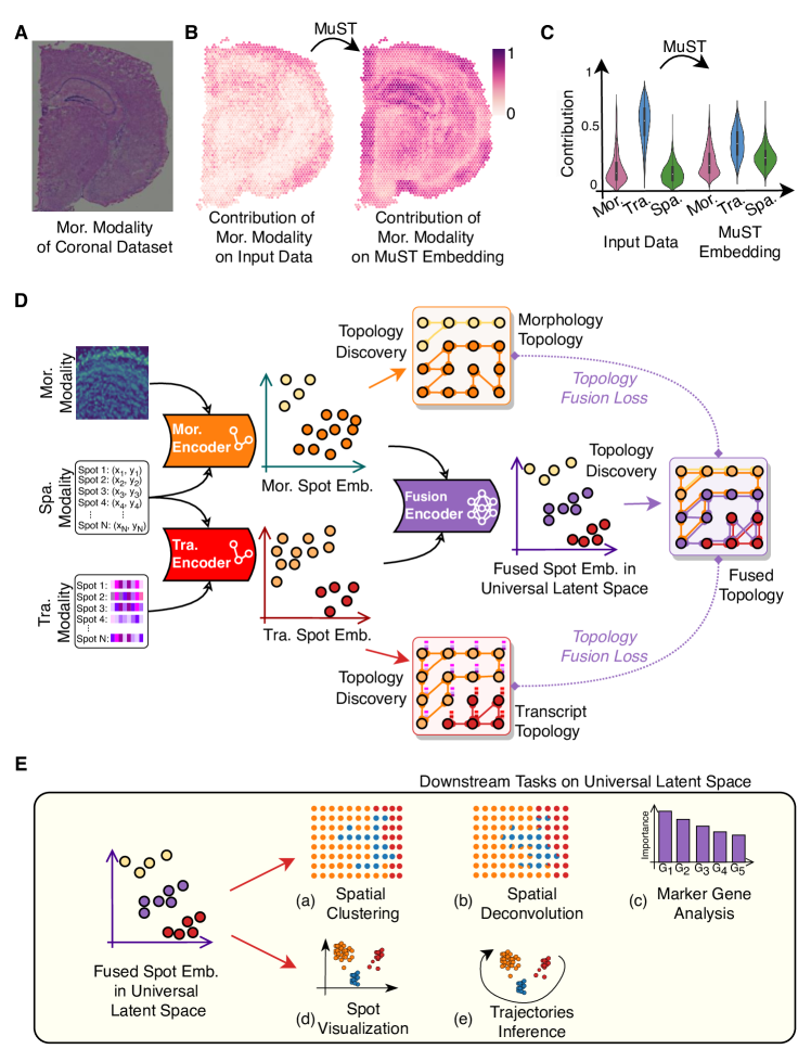
Figure 1: Illustration of MuST. A Morphology (Mor.) modality data of the coronal dataset. B Illustration of the modality bias phenomenon. In the case of Mor. modality, there is a significant inconsistency in the contribution of Mor. data to the final result (detected by Shapley value [42]). This inconsistency causes many methods to discard weaker modalities such as Mor. and Spa. resulting in a loss of information. MuST improves the retention of weaker modalities by mapping the Mor modality to the Transcriptomic (Tra.) modality. The results of the interpretable analyses show that the phenomenon of modality bias is mitigated by the Mor. Encoder processing. C The statistical evidence of the modality bias phenomenon is mitigated. D The ST data and its topologies of Tra. modalities, Mor. modalities and Spa. modalities are fused into a universal latent feature space (universal latent space) in which the information loss problems caused by the modality bias phenomenon are mitigated and the topologies of multimodal data are well represented. Specifically, the unit of ST data is called a ’spot’, and each spot contains Tra. data, Spa. data and Mor. data. MuST aims to map each spot into a vector of universal latent space in order to perform various downstream tasks. The Mor. and Tra. modality data are mapped to the single modal latent space feature by two graph encoders, with the spatial modal information used to construct the edges of the graph. The graph encoders represent each point of the ST data as a vector. The individual modal latent space features are then mapped to the universal latent space using a fusion encoder. The topology discovery operation extracts topological structures from the embedding by constructing KNN graphs (see Sec. 4.3), which express the topological relationships of the spot embedding. The topology fusion loss guides the network to learn a unified representation capable of fusing multimodal data, thereby improving performance in several downstream tasks. E Multiple downstream tasks. MuST incorporates information from multiple modalities and better supports multiple downstream tasks. These include (a) spatial clustering, (b) spot visualisation, (c) spatial deconvolution, (d) marker gene analysis, and (e) spatial trajectory inference. The mutual support of multiple downstream tasks allows for a more comprehensive understanding of ST data.

2.1 Overview of MuST

We observe that ST data suffer from the modality bias phenomenon. As shown in Fig. 1A-C, there is a significant inconsistent contribution to the data label among the morphology (Mor.) modality, transcriptomics (Tra.) modality and spatial (Spa.) modality. We use the interpretable method (Shapley Value [43, 42]) to show the differences in the contribution of data from different modalities to the ground truth (Sec. 4.2). As shown in Fig. 1B, in the coronal mouse brain dataset (Coronal), the contribution of the Mor. modality is not consistent, and in most regions the contribution of Mor. modality is negligible. However, in some specific tissue structures (e.g., hippocampus), the Mor. modality provides a stronger contribution. Furthermore, the violin plots in Fig. 1C show the statistical evidence of the modality bias phenomenon and it’s mitigation by MuST. The modality bias phenomenon causes some methods to ignore weaker modalities such as Mor. and Spa., resulting in a loss of information. Further evidence on Fig. 2 and Fig. 3 shows that modality bias phenomenon in contributions is common in ST data (Fig. 1C).

We propose MuST, a robust augmentation-based manifold learning ST method for several downstream tasks by fusing multiple modalities. MuST mitigates the modality bias phenomenon by introducing topology knowledge and a topology fusion loss function (evidence in Fig. 1B). MuST plays a crucial role in balancing the contributions of different modalities, thereby reducing information loss. The framework of MuST is shown in Fig. 1D. Specifically, MuST first fuses the Spa. information into the Mor./Tra. spot embedding space by the Mor./Tra. encoder. Then we fuse both Mor./Tra. spot embedding spaces into the universal latent space (fused spot embedding space) with the fusion encoder. We use a topology discovery strategy to accurately estimate global and local information for different modalities to discover the local connection in Mor./Tra. embedding spaces based on $k$-nearest neighbour ($k$NN). The superposition of local connections is then used to describe the global relationships of the data, i.e. a non-neighbouring point can be described by passing through several levels of neighbourhood relationships. To make the data distribution in the representation space more realistic, we dynamically generate new samples using neighbourhood-based interpolation and use the generated spots in the training process. Finally, we design topology fusion loss functions to fuse local and global information from different modalities using augmented data. (Fig. 4.3).

The universal latent space learned by MuST combines local and global information from different modalities to perform downstream tasks (Fig. 1E). Specifically, a spatial clustering task using clustering methods (e.g., mclust [44]), a spot visualisation task using visualisation methods (e.g., an MLP network based on topology loss [45] and UMAP [46]), marker gene analysis task using sensitivity analysis [47], spatial trajectory inference task using PAGA [22] method, and spatial deconvolution task using Lasso [48] method on the clustering results. The downstream tasks corroborate each other and provide a better understanding of the ST data. A comparison is made with several methods, including GraphST [15], STAGATE [25], DeepST [34], SpaGCN [31], MUSE [16], and stSME [32] based on mean relative rank error (MRRE) score, adjusted rand index (ARI) score, and biological significance analysis.

2.2 MuST Mitigates Modality Bias and Recognizes Complex Tissues on Mouse Brain Data

We initially assess MuST’s performance by its effectiveness in mitigating modality bias phenomenon and biological significance in mouse brain data. This evaluation confirms MuST’s proficiency in accurately identifying complex tissue structures. The datasets comprise three distinct modalities: Tra., Mor., and Spa., from two specific sections of the mouse brain - coronal mouse brain section and a mouse sagittal posterior brain section (Fig. 2B, H), acquired using the 10x Visium platform [49]. We compare the spatial domains identified by MuST with the corresponding anatomical reference annotations from the Allen Mouse Brain Atlas [50] (Fig. 2A, G), the goal is to verify our findings and assess the interpretative precision of MuST. Moreover, to ensure a higher resolution in our spatial clustering task, we set the number of clusters to $20$ for both datasets.

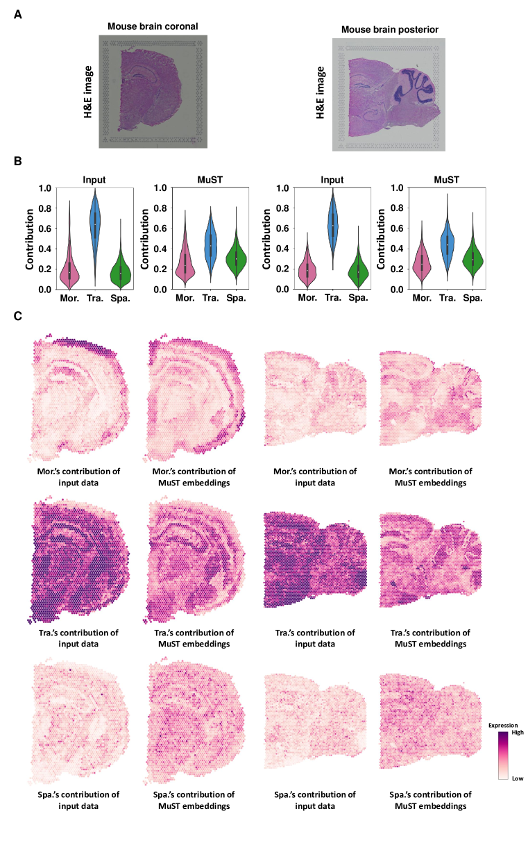
Figure S2: MuST alleviates the modality bias phenomenon in mouse brain data. A H&E image of mouse brain coronal section and mouse sagittal posterior brain section. B Contribution of the morphology (Mor.) modality, transcriptome (Tra.) modality and spatial (Spa.) modality input data or MuST embedding to data labeling. C Contribution visualization of the Mor. modality, Tra. modality and Spa. modality input data or MuST embedding to data labeling.

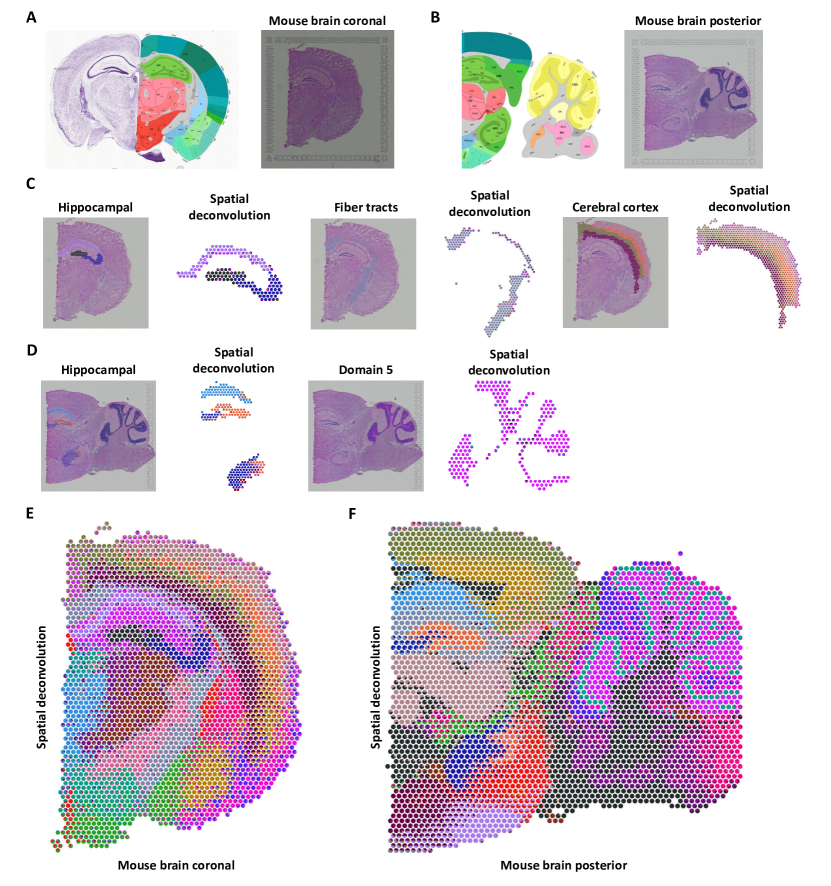
Figure S6: Spatial deconvolution of MuST’s results in adult mouse brain section profiled by 10x Visium. A Allen Brain Institute reference atlas diagram and H&E image of the mouse cortex. B Allen Brain Institute reference atlas diagram and H&E image of the mouse sagittal. C Spatial deconvolution of the identified domains by MuST on coronal mouse brain section. D Spatial deconvolution of the identified domains by MuST on mouse sagittal posterior brain section. E Spatial deconvolution of the coronal mouse brain section. F Spatial deconvolution of the mouse sagittal posterior brain section.

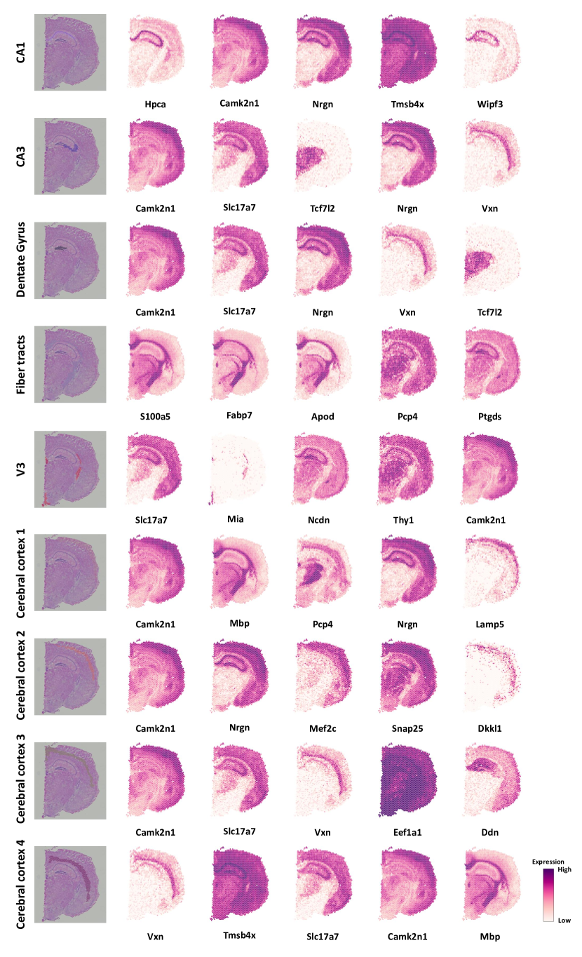
Figure S10: Marker genes selection for each region of coronal mouse brain section acquired with 10x Visium.

For the coronal mouse brain section, MuST better examine the hippocampal region, fiber tract region, cerebral cortex region, and V3 structure. The spatial domains identified by baseline methods roughly partition the tissue structures into groups containing different cell types while unable to identify small spatial domains (Fig. 2D). Specifically, all baseline methods fail to identify the V3 structure and “cordlike” structure (Ammon’s horn). stSME, SpaGCN, and DeepST fail to identify the “arrow-like” structure (dentate gyrus within the hippocampus). stSME, SpaGCN, MUSE, and DeepST fail to identify some small fiber tracts. In contrast, MuST brings noticeable enhancements in spatial domain identification (Fig. 2D). As follows, (1) In the hippocampal region, MuST identifies the CA1 field (domain 18) and CA3 field (domain 20) of the Ammon’s horn and the dentate gyrus structure (domain 6). The identified hippocampal region has high concordance with the selected marker genes Hpca (Fig. 2F, Tab. S6 and Fig. S10). These advantages may be attributed to the significant contribution of Tra. modality after MuST to Ammon’s horn and the dentate gyrus structure (Fig. S2C). (2) MuST better depicts the fiber tracts and groups the fiber tracts with texture structure in the histological image into one cluster (domain 16), which has high concordance with the selected marker genes Mbp (Fig. 2F). (3) In the cerebral cortex region, MuST identifies more cortical layers, including external (layers 2/3), internal (layer 4 and layer 5) and plexiform (layer 6) layers, and the thickness of the cerebral cortex is highly consistent with the anatomical reference annotations. This advantage is due to the combined contribution of Tra. modality (e.g., layers 4 and layer 6) and Mor. modality (e.g., layers 2/3 and layer 5) after MuST to the cerebral cortex (Fig. S2C), thus validating the ability and significance of MuST to mitigate modality bias phenomenon (Fig. 2C). The identified cerebral cortex region concurs highly with the selected marker gene Camk2n1 (Fig. 2F). (4) MuST accurately identifies the V3 structure (domain 4), which is not possible with baseline methods. The Fabp7 gene expression is well alignment with the identified V3 structure (Fig. S10). In the visualization results (Fig. 2E), MuST also separates these tissue structures marked with a dashed circle. In the spatial deconvolution task, the cluster compositions inferred by MuST also accurately depict the regions identified by MuST (Fig. S6C, E).

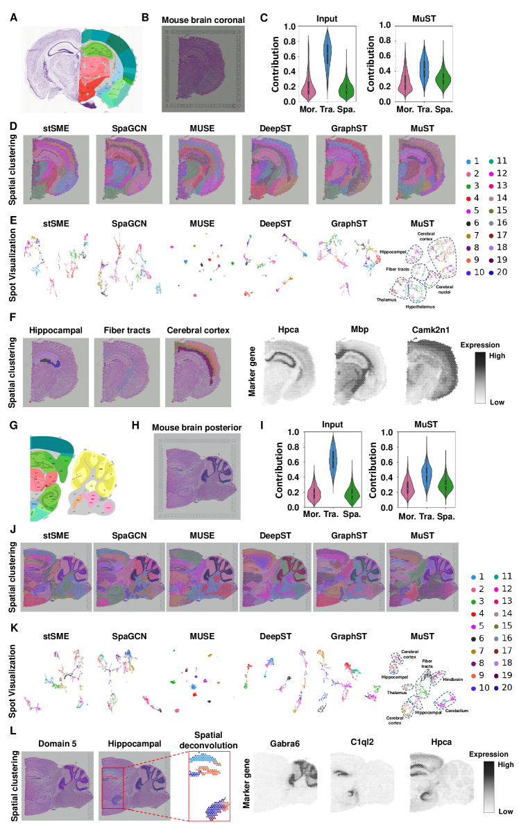
Figure 2: MuST explores more biologically complex tissues in adult mouse brain section profiled by 10x Visium (10x Genomics). A The annotation of hippocampus structures from the Allen Reference Atlas of an adult mouse brain. B H&E image of mouse brain coronal section. C Contribution of the morphology (Mor.) modality, transcriptome (Tra.) modality and spatial (Spa.) modality input data or MuST embedding to data labeling. D Clustering results by spatial methods, stSME, SpaGCN, MUSE, DeepST, GraphST, and MuST. E Spot visualization generated by the spatial methods. F Single cluster visualization of spatial domains identified by MuST and the corresponding marker gene expressions. G Allen Brain Institute reference atlas diagram of the mouse sagittal. H H&E image of mouse sagittal posterior brain section. I Contribution of the Mor. modality, Tra. modality and Spa. modality input data or MuST embedding to data labeling. J Clustering results by spatial methods, stSME, SpaGCN, MUSE, DeepST, GraphST, and MuST. K Spot visualization generated by the spatial methods. L Single cluster visualization of spatial domains identified by MuST and the corresponding marker gene expressions and cluster-related spatial deconvolution.

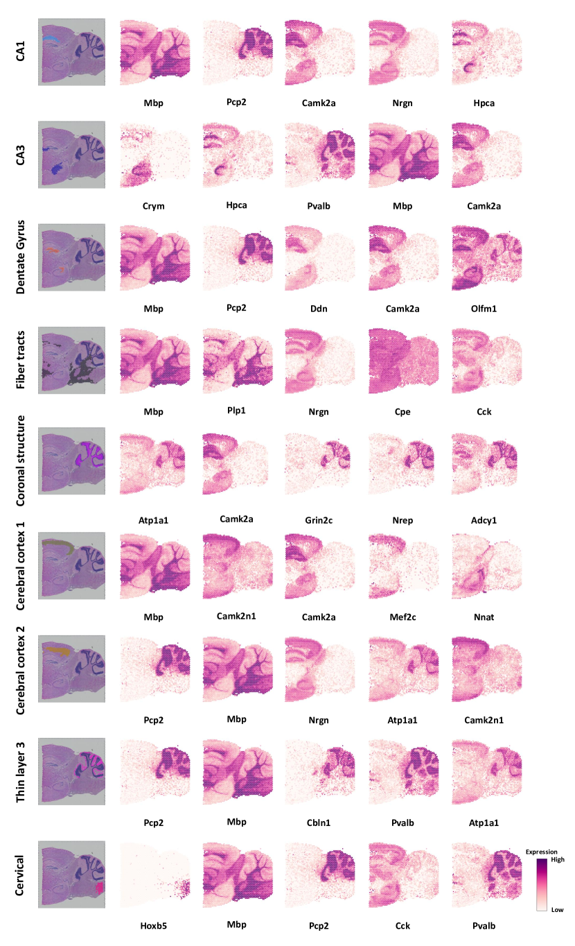
Figure S11: Marker genes selection for each region of mouse sagittal posterior brain section acquired with 10x Visium.

For the mouse sagittal posterior brain section, MuST better examines the hippocampal region and coronal structure. The baseline methods cannot also identify small spatial domains (Fig. 2J). Specifically, they fail to identify the “cordlike” structure, “arrow-like” structure, and the thin layer around the coronal structure. In contrast, MuST better alleviates the problems existing in these methods (Fig. 2J). (1) In the hippocampal region, MuST identifies the CA1 field (domain 1) and CA3 field (domain 20) of the Ammon’s horn, which has high concordance with marker gene Hpca (Fig. 2L, Tab. S7 and Fig. S11). MuST can group the dentate gyrus structure (domain 9) into one cluster with high concordance with the selected marker gene C1ql2 (Fig. 2L). The cluster compositions inferred by MuST also accurately depict the identified hippocampal region (Fig. 2L and Fig. S6D, F). These advantages may be attributed to the significant contribution of Tra. modality after MuST to “cordlike” structure and “arrow-like” structure (Fig. S2C). (2) MuST can depict the coronal structure and thin layer around it (domains 5, 11, and 12), and MuST is the only method that can clearly distinguish these three domains, which correspond to the texture structure of histological image. This advantage is due to the combined contribution of Tra. modality (e.g., thin layer around the coronal structure) and Mor. modality (e.g., coronal structure) after MuST to this region (Fig. S2C), thus validating the ability and significance of MuST to mitigate modality bias phenomenon (Fig. 2I). The Gabra6 expression aligns well with the identified spatial domain (Fig. 2L). In the visualization results, MuST significantly improves the separation of tissue structures (e.g., cerebellum, thalamus, cerebral cortex, hindbrain, and fiber tracts) (Fig. 2K) mentioned above, this verifies that the universal latent space, which can better fuse information from multiple modalities, is beneficial for various downstream tasks.

2.3 MuST Distinctly Recognizes Fine-grained Tissue Structures on Mouse Embryo Data

Building on our preliminary evaluation of MuST in mouse brain data, which involves assessing its capability to mitigate modality bias across three modalities and its biological significance. We now broaden our research scope to encompass Stereo-seq [10] datasets from mouse embryos at developmental stages E14.5 (Fig. 3A) and E9.5 (Fig. 3F). This phase of evaluation specifically concentrates on mitigating modality bias, particularly in Tra. modality and Spa. modality, within the context of large-scale data. The tissue domain annotations for these datasets are obtained from the original study [10].

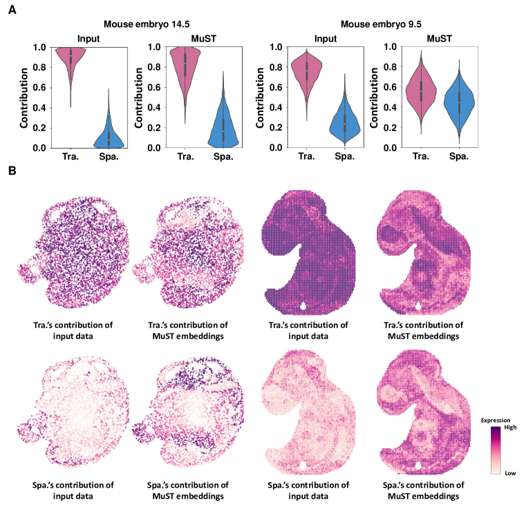
Figure S3: MuST alleviates the modality bias phenomenon in mouse embryo data. A Contribution of the morphology (Mor.) modality, transcriptome (Tra.) modality and spatial (Spa.) modality input data or MuST embedding to data labeling on mouse embryo 14.5 and 9.5 datasets. C Contribution visualization of the Mor. modality, Tra. modality and Spa. modality input data or MuST embedding to data labeling.

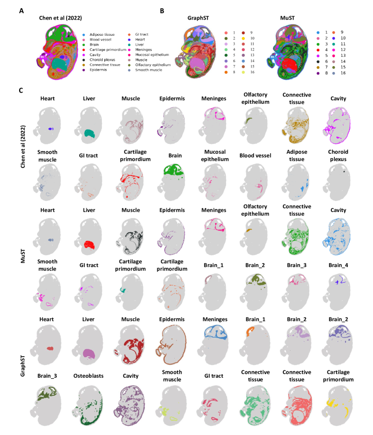
Figure S4: MuST enables accurate identification of different organs in the Stereo-seq mouse embryo. A Tissue domain annotations of the E14.5 mouse embryo data obtained from the original Stereo-seq study. B Clustering results by GraphST and MuST on the E14.5 mouse embryo. C Cluster visualization of selected spatial domains identified by the original Stereo-seq study, MuST and GraphST, respectively.

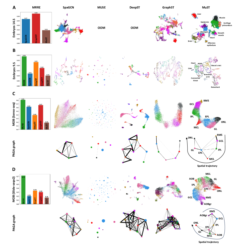
Figure S7: Embedding analysis of MuST on the mouse olfactory bulb tissue and mouse embryo. A Mean relative rank error (MRRE) scores and UMAP visualizations generated by SpcGCN, MUSE, DeepST, GraphST and MuST representations on the Stereo-seq E14.5 mouse embryo data. Among them, methods MUSE and DeepST have an out of memory (OOM) problem. B MRRE scores and spot visualizations generated by the representations of five methods on the Stereo-seq E9.5 mouse embryo data. C MRRE scores, spot visualizations and PAGA graphs generated by the representations of five methods on the Stereo-seq mouse olfactory bulb tissue section. D MRRE scores, spot visualizations and PAGA graphs generated by the representations of five methods on the Slide-seqv2 mouse olfactory bulb tissue section.

For the E14.5 mouse embryo, MuST better recovers the olfactory epithelium and cartilage primordium region. We set the number of clusters to $16$ to match the original annotation for the spatial clustering task (Fig. 3A). MuST, GraphST and SpaGCN capture much of the fine-grained structure in the embryo and accurately identify major areas, such as the heart, liver, muscle, epidermis, and meninges regions (Fig. 3A). Furthermore, MuST captures more of the fine-grained structures (Fig. S4C), such as the olfactory epithelium and cartilage primordium regions (Fig. 3E). As follows, (1) MuST better demarcates olfactory epithelium as a separate region [15], consistent with the original annotation, whereas GraphST clusters it as part of the brain region and SpaGCN assigns part of the mucosal epithelium region to it. In the visualization space (Fig. 3B and Fig. S7A), MuST also separates the olfactory epithelium region labeled by a dashed circle [45]. The identified olfactory epithelium region has high concordance with the selected marker genes Ugt2a2 and Sult1e1 (Fig. 3E and Tab. S3). The cluster compositions inferred by MuST accurately depict the identified olfactory epithelium region (Fig. 3E). These advantages may be attributed to the significant contribution of Tra. modality after MuST to olfactory epithelium region (Fig. S3B). (2) MuST better demarcates the cartilage primordium region around the brain, which has high concordance with the selected marker genes Col11a1 and Col2a1 (Fig. 3E). MuST also separates the cartilage primordium region labeled by a dashed circle (Fig. 3B). The cluster compositions inferred by MuST accurately depict the identified cartilage primordium region (Fig. 3E). In addition, MuST obtains the best MRRE score $0.15$ compared with GraphST ($0.33$) and SpaGCN ($0.27$) (Fig. 3C).

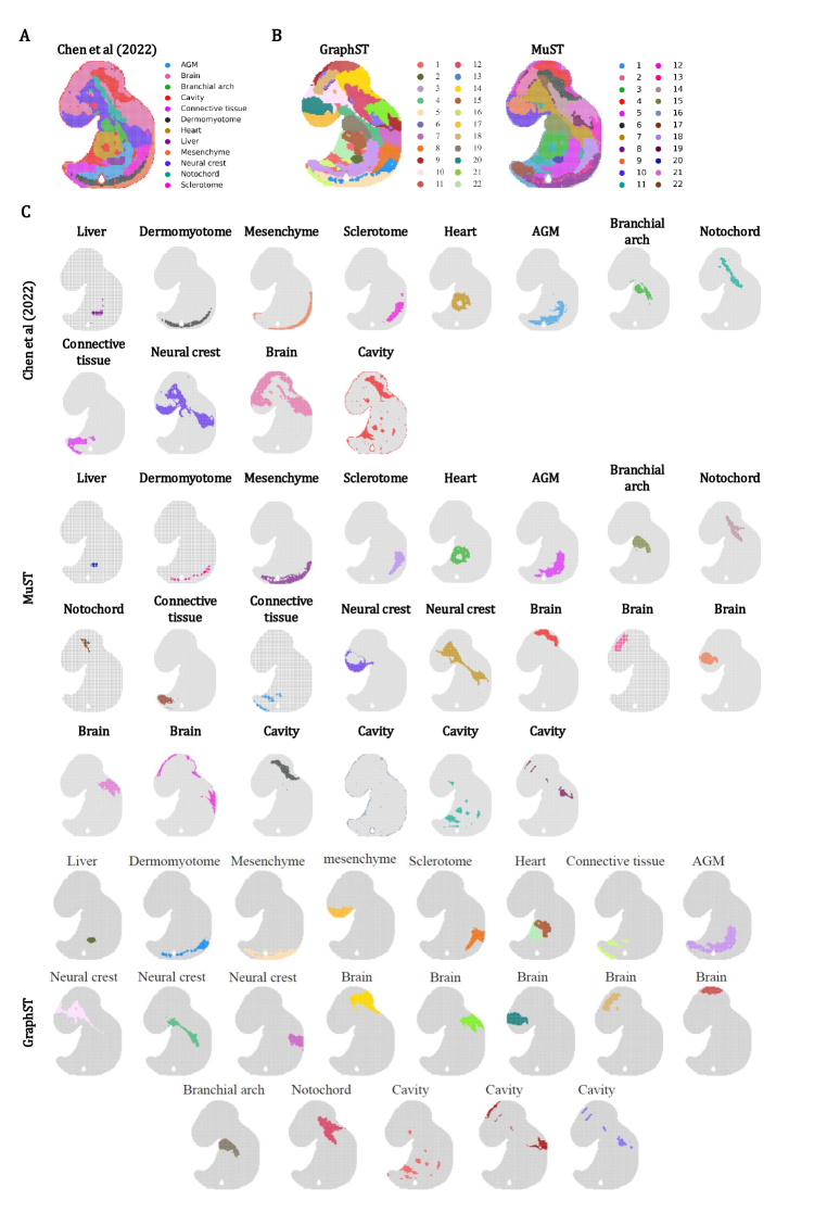
Figure S5: MuST enables accurate identification of different organs in the Stereo-seq mouse embryo. A Tissue domain annotations of the E9.5 mouse embryo data obtained from the original Stereo-seq study. B Clustering results by GraphST and MuST on the E9.5 mouse embryo. C Cluster visualization of selected spatial domains identified by the original Stereo-seq study, MuST and GraphST, respectively.

For E9.5 mouse embryo, MuST better recovers the heart, neural crest, connective tissue, and notochord regions. Although the original annotation has $12$ reference clusters (Fig. 3F), the number of clusters in our testing is set to $22$ for the spatial clustering task to acquire a higher resolution of tissue segmentation [15]. Some clusters of GraphST and SpaGCN match the annotated regions (Fig. 3F), such as liver region, but the contours of mesenchyme, sclerotome, and AGM regions are not accurate. In contrast, MuST further captures much of the fine-grained and contours structures, including heart, neural crest, notochord, connective tissue, brain, and cavity regions (Fig. 3F and Fig. S5C), and are highly concordant with the original annotation. As follows, (1) MuST demarcates the heart region as a separate cluster, consistent with the original annotation, whereas GraphST divides it into two clusters. In the visualization results, MuST also separates the heart region labeled by a dashed circle (Fig. 3G and Fig. S7B). The identified heart region has high concordance with the selected marker genes Myl7, Actc1, and Acta1 (Fig. 3J and Tab. S4). The cluster compositions inferred by MuST accurately depict the identified heart region (Fig. 3J). These advantages may be attributed to the significant contribution of Tra. modality after MuST to heart region (Fig. S3B). (2) MuST better describes the contours of the notochord region and more completely demarcates the connective tissue region, whereas SpaGCN assigns part of the AGM region to connective tissue region. The identified connective tissue region concurs highly with the selected marker genes Postn and Hbb-bs (Fig. 3J). This advantage is due to the combined contribution of Tra. modality and Loc. modality after MuST to connective tissue region (Fig. 3I and Fig. S3B). (3) MuST better demarcates the neural crest region, whereas GraphST assigns part of the mesenchyme and brain regions to this region. In addition, MuST obtains best MRRE score $0.10$, followed by SpaGCN ($0.12$) and GraphST ($0.18$) (Fig. 3H). The evaluation of universal latent space representations helps us to explain the above analysis and verifies the effectiveness of modality fusing ability in MuST.

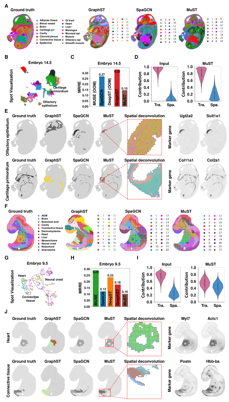
Figure 3: MuST enables accurate identification of different organs in the Stereo-seq mouse embryo (MOSTA). A Tissue domain annotations obtained from the original Stereo-seq study and clustering results by GraphST and MuST on the E14.5 mouse embryo data. B Spot visualizations generated by MuST representations. C MRRE scores generated by MUSE, SpaGCN, DeepST, GraphST, and MuST representations. Among them, methods MUSE and DeepST have an out-of-memory (OOM) problem. D Contribution of the transcriptome (Tra.) modality and spatial (Spa.) modality input data or MuST embedding to data labeling. E Single cluster visualization of selected spatial domains identified by the original Stereo-seq study, GraphST and MuST, and the corresponding spatial deconvolution and marker genes of selected spatial domains identified by MuST. F Tissue domain annotations obtained from the original Stereo-seq study and clustering results by GraphST and MuST on the E9.5 mouse embryo data. G Spot visualizations generated by MuST representations. H MRRE scores generated by MUSE, SpaGCN, DeepST, GraphST, and MuST representations. I Contribution of the Tra. modality and Spa. modality input data or MuST embedding to data labeling. J Single cluster visualization of selected spatial domains identified by the original Stereo-seq study, GraphST and MuST, and the corresponding spatial deconvolution and marker genes of selected spatial domains identified by MuST.

2.4 MuST Distinctly Recognizes Anatomical Regions on Mouse Hippocampus Data

Building on the insights gained from the analysis of the 10x Visium and Stereo-seq platform, we extend our investigation to more advanced platform SlideseqV2 [9]. This progression allows us to explore the consistency of spatial transcriptomic patterns across different technological iterations and the robustness of MuST. For this comparison, we employ the annotated Allen Brain Atlas as the ground truth [50] (Fig. 4A).

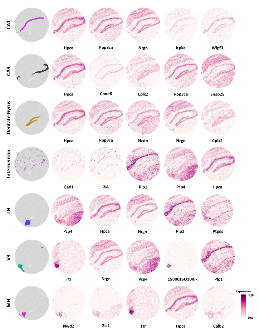
Figure S9: Marker genes selection for each anatomical region of mouse hippocampus data acquired with SlideseqV2.

MuST produces more spatially consistent clustering and captures major anatomical regions, such as the dentate gyrus and the pyramidal layers within Ammon’s horn (CA1 and CA3 regions), and MuST better discerns the cavity tissue structure and the region covered by interneuron cells. We set the number of clusters in our testing to $13$ to acquire a higher resolution of tissue segmentation (Fig. 4B). Specifically, (1) MuST and GraphST are better than STAGATE in delineating the CA3 and dentate gyrus regions with sharper boundaries. MuST and STAGATE demarcate more neocortical layers in the cerebral cortex, and GraphST groups them into one region. (2) MuST and GraphST can differentiate between the third ventricle (V3), medial habenula (MH), and lateral habenula (LH), which have high concordance with their marker genes Enpp2, Nwd2, and Gpr151, respectively (Fig. 4D, Tab. S5 and Fig. S9). The cluster compositions inferred by MuST accurately depict the identified V3, MH, and LH regions (Fig. 4G and Fig. 4E). However, STAGATE merges the MH and LH into one region. For the V3 structure, the Enpp2 expression does not align well with the detected V3 region of MuST (Fig. 4D), but the latter better resembles the V3 region in the annotated brain reference (Fig. 4A). For comparison, the V3 regions of STAGATE are closer to the shape of the Enpp2 expression region but do not match the anatomical shape well. In the visualization results, MuST also separates the V3, MH, and LH regions (Fig. 4C). (3) MuST can discern the cavity tissue structure and interneuron cell regions. The cavity region has higher concordance with the anatomical annotation (Fig. 4A), and the interneuron cell region concurs more with the selected marker gene Sst (Fig. 4F). Then, we use the MRRE score to explain the above analysis quantitatively (Fig. 4H). MuST obtains the best MRRE score $0.13$, while GraphST ($0.45$) and STAGATE ($0.41$) get much worse performance.

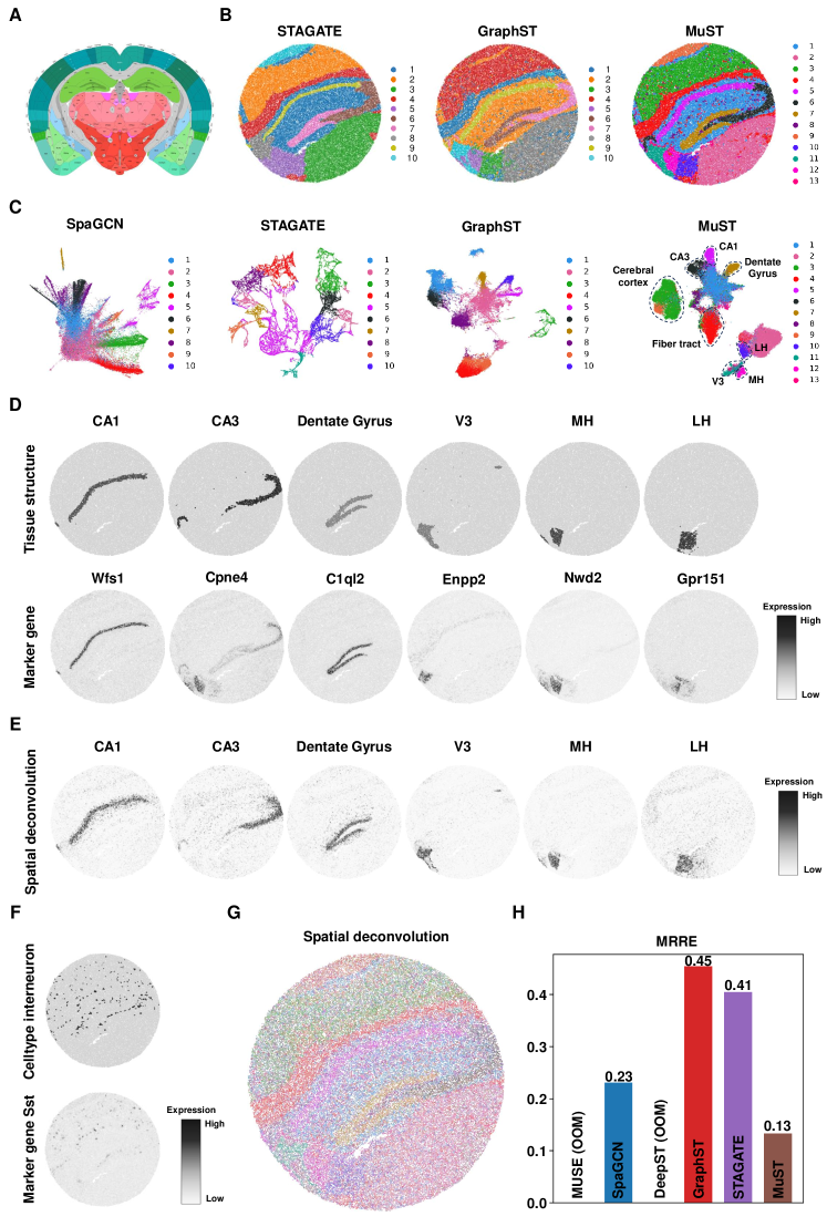
Figure 4: MuST discerns relevant anatomical regions more accurately in the SlideseqV2 mouse hippocampus data (SCP354). A Allen Brain Institute reference atlas diagram of the mouse cortex. B Clustering results by spatial methods, STAGATE, GraphST and MuST on the mouse hippocampus data. C Spot visualizations generated by SpaGCN, STAGATE, GraphST and MuST representations. D Single cluster visualization of the tissue structures identified by MuST and the corresponding marker gene expressions. E Cluster-related spatial deconvolution analysis of the tissue structures identified by MuST. F Visualization of the celltype identified by MuST and the corresponding marker gene expressions. G Cluster-related spatial deconvolution analysis. H MRRE scores generated by SpaGCN, GraphST, STAGATE, and MuST representations.

2.5 MuST Recognizes Laminar Structure on Mouse Olfactory Bulb Data

Building on the discussion of the block structure analysis performed on three different platforms, we now turn our attention to evaluating the capabilities in analyzing hierarchical/laminar structures. Because a clear delineation of the laminar structure can only be achieved by reasonably fusing the information provided by different modalities.

We use two mouse olfactory bulb tissue datasets acquired with high-resolution platforms Stereo-seq [10] and Slide-seqV2 [9], to rigorously test MuST’s proficiency in delineating intricate laminar architectures. For the former, we compare the spatial domains identified by MuST with the mouse olfactory bulb’s laminar structure annotated by the DAPI-stained image [51, 25], identifying the olfactory nerve layer (ONL), glomerular layer (GL), external plexiform layer (EPL), mitral cell layer (MCL), internal plexiform layer (IPL), granule cell layer (GCL), and rostral migratory stream (RMS) (Fig. 5A). For the latter, we compare the spatial domains identified by MuST with the laminar organization of mouse olfactory bulb annotated by the Allen Reference Atlas [50], identifying the accessory olfactory bulb (AOB), granular layer of the accessory olfactory bulb (AOBgr), RMS, GCL, IPL, MCL, EPL, GL, and ONL (Fig. 5D).

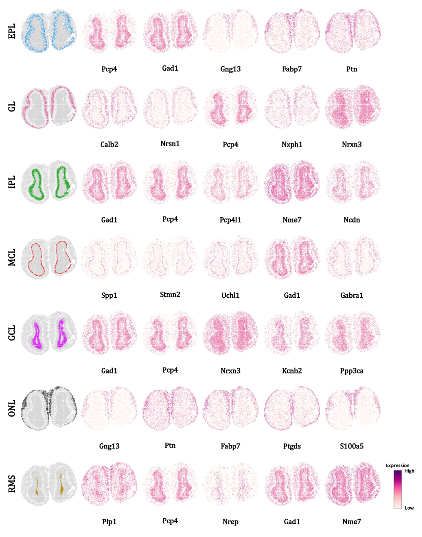
Figure S12: Marker genes selection for each laminar organization of coronal mouse olfactory bulb tissue datasets acquired with Stereo-seq.

For mouse olfactory bulb tissue section acquired with Stereo-seq, MuST more clearly recognizes the external and internal structure of the organ. We set the number of clusters to $7$ to match the known laminar structure for the spatial clustering task. STAGATE, GraphST, and MuST can separate the outer layers of the organ, namely the ONL, GL, and EPL, but STAGATE seriously confuses GL and EPL structures (Fig. 5B). MuST and GraphST can demarcate the GCL and RMS structures for the inner structure. However, GraphST’s clusters are noisy, and the boundaries between different structures are not as straightforward as MuST. We use the respective selected marker genes of each anatomical region to validate MuST’s clusters (Fig. 5C), and find the excellent correspondence between MuST’s clusters and the known marker genes (Tab. S8 and Fig. S12), such as Gabra1 [39], Cck and Ptn. For some marker genes (e.g., Ppp3ca and Pcp4), their high expression levels overlap with neighboring regions. This is expected as cell types are often shared among the different inner structures of organs, and markers are likewise shared among similar cell types. MuST delineates the spatial trajectory among the mouse olfactory bulb (from RMS to GCL to ONL) with clear boundaries between different structures in the visualization results as well as the PAGA graphs [22] (Fig. 5G), but other methods do not have this capability (Fig. S7C). In addition, MuST obtains the best MRRE score 0.19 (Fig. 5H), while MUSE (0.81) and GraphST (0.67) get much worse performance.

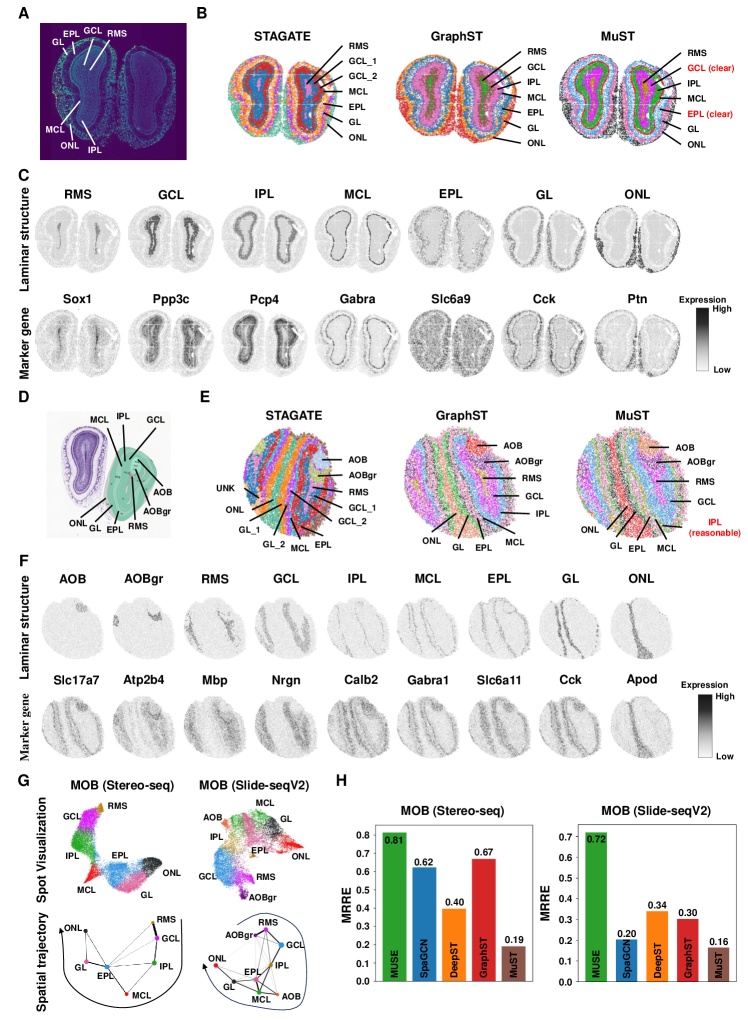
Figure 5: MuST identifies the laminar organization in the mouse olfactory bulb tissue sections profiled by Stereo-seq (SEDR) and Slide-seqV2 (SCP815) respectively. A Laminar organization of mouse olfactory bulb annotated in the DAPI-stained image generated by Stereo-seq. B Clustering results by spatial methods, STAGATE, GraphST and MuST on the Stereo-seq mouse olfactory bulb tissue section. C Single cluster visualization of the spatial domains identified by MuST and the corresponding marker gene expressions. D Laminar organization of mouse olfactory bulb annotated by the Allen Reference Atlas. E Clustering results by spatial methods, STAGATE, GraphST and MuST on Slide-seqv2 mouse olfactory bulb tissue section. F Single cluster visualization of spatial domains identified by MuST and the corresponding marker gene expressions. G Spot visualizations and PAGA graphs generated by the representations of MuST. H MRRE scores generated by MUSE, SpaGCN, DeepST, GraphST, and MuST representations.

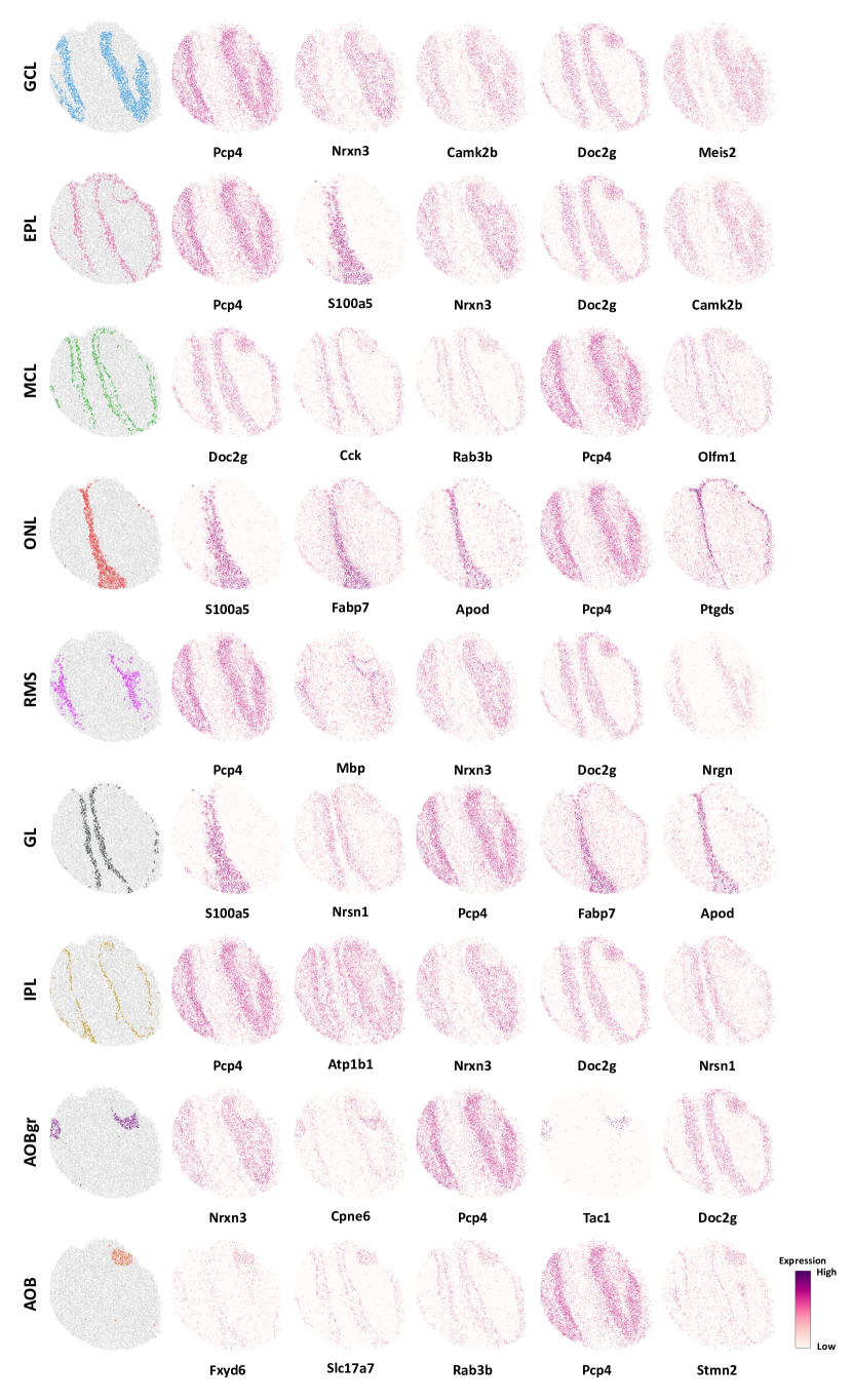
Figure S13: Marker genes selection for each laminar organization of coronal mouse olfactory bulb tissue datasets acquired with Slide-seqV2.

For mouse olfactory bulb tissue section acquired with Slide-seqV2, MuST better recognizes the laminar structure using fewer clusters. We set the number of clusters to $9$ to match the known laminar structure for the spatial clustering task. The spatial domains identified by MuST are consistent with the mouse olfactory bulb annotation from the Allen Reference Atlas. At the same time, baseline methods need more clusters to identify these structures (Fig. 5E). These spatial domains uncovered by MuST are clearly supported by known and selected gene markers (Fig. 5F, Tab. S9 and Fig. S13). The granular cell marker Atp2b4 [52] shows strong expressions on the identified AOBgr domain. MuST identifies the GCL structure with the dominant expression of Nrgn [40]. Nrgn is a well-documented schizophrenia risk gene, implying that this domain is related to cognition function. The narrow MCL structure with the dominant expression of mitral cell marker Gabra1 [39] is also identified by MuST. MuST delineates the spatial trajectory among the mouse olfactory bulb (from AOBgr to RMS to ONL) in the visualization results and the PAGA graphs (Fig. 5G), but other methods do not have this capability (Fig. S7D). In addition, MuST obtains the best MRRE score of 0.16, while MUSE (0.72) and GraphST (0.48) get much worse performance (Fig. 5H). Collectively, these results illustrate the modalities fusing ability of MuST to identify tissue structures and reveal their organization from ST data of different spatial resolutions.

2.6 MuST Exploratively Recognizes Layers on Human Dorsolateral Prefrontal Cortex Data

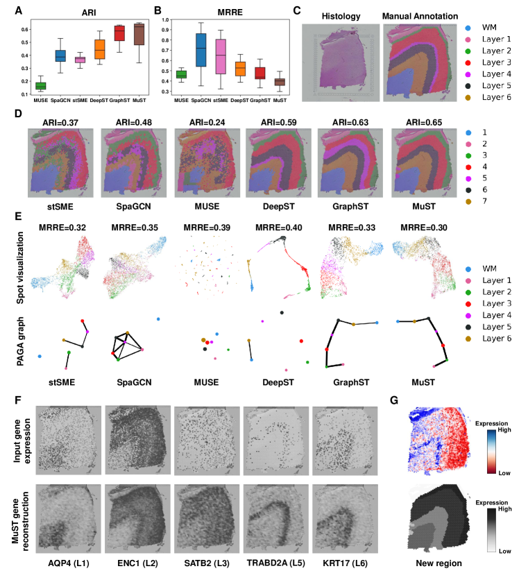
Figure 6: MuST improves the identification of layer structures in the human dorsolateral prefrontal cortex (DLPFC) tissue (spatialLIBD). A Boxplots of adjusted rand index (ARI) scores of six spatial methods applied to the 12 DLPFC slices. Boxplots denote medians and interquartile ranges (IQRs). The whiskers of a boxplot are the lowest datum still within 1.5 IQR of the lower quartile and the highest datum within 1.5 IQR of the upper quartile. B Boxplots of mean relative rank error (MRRE) scores of six spatial methods applied to the 12 DLPFC slices. C H&E image and manual annotation from the original study. D Clustering results by spatial methods, stSME, SpaGCN, MUSE, DeepST, GraphST, and MuST on slice 151673 of the DLPFC dataset. Manual annotations and clustering results of the other DLPFC slices are shown in supplementary information Fig. S8. E Spot visualizations and PAGA graphs generated by stSME, SpaGCN, MUSE, DeepST, GraphST, and MuST representations on slice 151673. F Visualizations of the input gene expressions and MuST gene reconstructions of five layer-marker genes on slice 151673. G Gene expressions analysis of the new regions.

Having established MuST’s efficacy in analyzing block structures in mouse data, we extend our investigation to human datasets to assess its broader applicability. This transition from model organisms to human data is crucial for validating MuST’s utility in more complex and clinically relevant settings.

We apply MuST to LIBD human dorsolateral prefrontal cortex (DLPFC) dataset [41], which contains ST profiles of $12$ DLPFC slices and each depicting the four or six layers of the human dorsolateral prefrontal cortex and white matter (WM). Across $12$ slices, for ARI score (Fig. 6A), MuST achieves the highest median score $0.62$, GraphST obtains the second median score $0.59$ after MuST, MUSE obtains the poorest median score $0.16$, and the remaining methods have median ARI scores of less than $0.44$. For MRRE score (Fig. 6B), MuST achieves best median score $0.40$, GraphST obtains the second median score $0.44$, and the MRRE median scores of SpaGCN ($0.72$) and stSME ($0.65$) are worse. We illustrate the results with one slice 151673 (Fig. 6D-G).

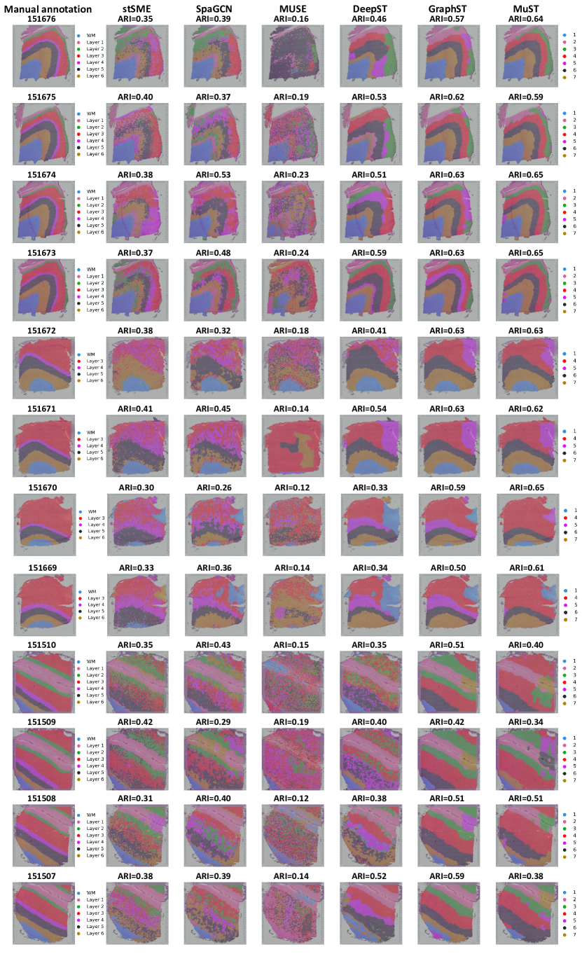
Figure S8: Manual annotations and comparison of spatial domains identified by stSME, SpaGCN, MUSE, DeepST, GraphST and MuST on the 12 slices of DLPFC dataset.

MuST achieves more competitive performance on spatial clustering tasks than baseline methods. The visual comparisons clearly show that the MUSE performs the worst spatial clustering, failing to identify every slice layer 151673. stSME and SpaGCN slightly alleviate the problem existing in MUSE with the ability to recover WM, but with the remaining clusters mixed among six layers, including the WM has a broken boundary and being clustered together with a portion of Layer 6, and the boundaries between other clusters are also very chaotic with no clean separation. DeepST accomplishes better separation of each layer, but with incorrect layer thickness, fails to recover Layer 4, and the boundaries between WM and Layer 6 still need to be more apparent. GraphST and MuST produce layers that are significantly closer in shape to the manual annotation (Fig. 6C), but with some minor flaws. GraphST fails to recover Layer 2, and the thickness of Layer 1 and Layer 4 are not accurate, while MuST successes to recover Layer 2 and better captures the position and thickness (Fig. 6D). MuST fails to identify Layer 4, which is understandable because Layer 4 is usually skinny and contains similar cell types to Layer 3, such as pyramidal neurons. Therefore, MuST discovers a new spatial domain that differs significantly in gene expression from the others (Fig. 6G). For quantitative assessment, MuST achieves the highest ARI score of 0.65, GraphST obtains the second highest ARI score of 0.63, while the MUSE is the poorest method at an ARI score of 0.24. The results with all other slices are shown in Fig. S8.

MuST effectively incorporates Spa. modality in the data, which allows it to reflect the distance between spatial domains and capture spatial trajectory in the visualization results [46]. For example, in slice 151673, the different cortical layers appear well-organized and follow a clear spatial trajectory (from Layer 1 to Layer 6 to WM) in the visualization results (Fig. 6E). This result is consistent with the functional similarity between adjacent cortical layers and the chronological order [53]. By contrast, in the visualization results of MUSE embeddings, spots belonging to the same layers are split into multiple clusters. As for the other spatial clustering methods, stSME mixes the spots of layer 1 (green) and other cortex layers, and SpaGCN does not distinguish Layer 4 and other cortex layers clearly. We additionally validate the inferred spatial trajectory utilizing PAGA (Fig. 6E). The PAGA graphs of MuST and GraphST representations show an almost linear development trajectory from Layer 1 to Layer 6 and the similarity between adjacent layers. In contrast, the PAGA result of both SpaGCN representations is mixed to different degrees, and the PAGA results of stSME, MUSE, and DeepST representations cannot recover spatial trajectories. For quantitative assessment, MuST achieves the lowest MRRE score of 0.30, while the DeepST is the poorest method at an MRRE score of 0.40. In addition, MuST can denoise the gene expressions based on the universal latent space. We apply MuST to decrease noises in the DLPFC dataset to better show the spatial pattern of genes across the layers of the cortex. We compare the expression profiles of five layer-marker genes of the input data to the denoised representations by MuST in the slice 151673 in Fig. 6F. As anticipated, the MuST-denoised representations clearly show the laminar enrichment of these layer-specific marker genes. For example, after denoising, the AQP4, ENC1, SATB2, TRABD2A, and KRT17 genes [41] show differential expressions in Layer 1, Layer 2, Layer 3, Layer 5, and Layer 6 respectively, which are consistent with previously reported results.

3 Discussion

This paper introduces MuST, a augmentation-based manifold learning model that integrates gene expression, tissue morphology, and spatial information into a latent model for a variety of downstream tasks, including spatial clustering [15, 16], spot visualization [17, 18], spatial deconvolution [19, 20], marker gene analysis [21], and spatial trajectory inference [22], with improved precision.

MuST mitigates the detrimental effects of modality bias and therefore has a robust modality integration capability. The information in the weaker modalities (Mor. modality and Spa. modality) is better exploited to characterise and improve the performance of various downstream tasks. As an indication of the benefits of these techniques, MuST exploits morphological and textural differences to improve the identification of key tissue structures. For example, in the coronal mouse brain dataset and the sagittal mouse posterior brain dataset (Sec. 2.2 and Fig. 2) [49], MuST more accurately detects morphological variations, which sharpens the distinction of hippocampal region, cerebral cortex region and coronal structure. However, GraphST [15] fails to identify the “string-like” and “arrow-like” structures due to its neglect of morphological information. The coarse-grained detection of hippocampal structure by other methods (e.g., stSME [32], SpaGCN [31] and DeepST [34]) may be due to the negative effect of the modality bias. Furthermore, in the human DLPFC dataset (Sec. 2.6 and Fig. 6) [41], MuST more effectively recognises the texture structure (cluster 2 in Fig. 6D) in histology images, while GraphST neglects this information. MuST is also better at recovering the fine-grained tissue structures in mouse embryo datasets due to the integration of Spa. and Tra. modalities (Sec. 2.3 and Fig. 3). It handles large data sets, although the stereo-seq technology does not provide data for the Mor. modality. However, the modality bias leads to inaccurate results from other methods (e.g. olfactory epithelium, cartilage primordium, heart, neural crest, notochord, connective tissue, brain and cavity regions) compared to the ground truth.

Another advantage of MuST is its ability to perform synergistic analysis across multiple downstream tasks, potentially yielding consistent, confirmatory results. In spatial clustering, MuST identifies distinct regions such as olfactory epithelium, cartilage primordium, heart, notochord and connective tissue in embryo data (Sec. 2.3), and hippocampal areas (e.g. CA1, CA3, dentate gyrus), fibre tracts, cerebral cortex and V3 structures in mouse brain data (Sec. 2.2). At the same time, some regions (e.g. olfactory epithelium, hippocampus, fibre tracts, cerebral cortex) are also delineated in the visualisation subtask, revealing intricate details of tissue similarity. Building on this universal latent space, spatial clustering and spot visualisation guide the interpretability and feature selection task to focus on specific genes associated with the identified differences. For example, the unity between the tagged regions and selected marker genes - Ugt2a2 and Sult1e1 in the olfactory epithelium region, Myl7 and Actc1 in the heart region (Sec. 2.3), and C1ql2 and Hpca in the hippocampus region (Sec. 2.2) - is evident. The cluster compositions derived from MuST accurately characterise these regions. These downstream tasks show remarkable consistency in biological significance, outperforming other baseline methods.

Ultimately, MuST is versatile, processing ST data from a variety of platforms, such as 10x Visium [7], Slide-seqV2 [9] and Stereo-seq [10], and effectively managing the different spatial resolutions inherent in these technologies. In the future, we plan to extend MuST to build a pre-trained base model to provide a foundation not only for the tasks considered in this work, but also for other related tasks, including solving batch effect problems through graph structure integration, annotating cell types, and interpreting developmental trajectories. Due to its broad applicability, flexibility and potential for extension, we anticipate that MuST will become an indispensable tool in ST research.

4 Methods

4.1 Data Preprocessing

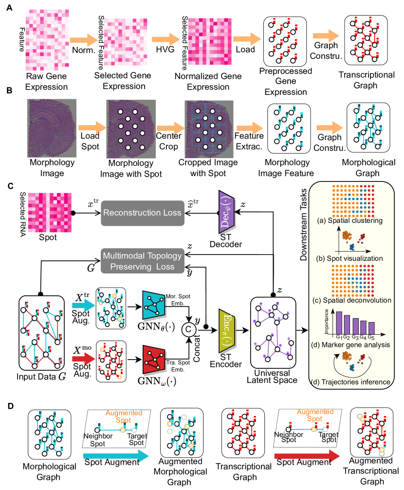
Figure S1: Details framework of MuST. A. Preprocessing for transcriptomics modality. The gene expression counts are log transformed and normalised and then we select the 3000 most variable genes. B. Preprocessing for morphology modality. We centre and crop a $224\times 224$ pixel area around the probe coordinates. These images are then processed by the ResNet50 architecture [56], to distill a 2048-dimensional feature vector and use PCA map the 2048-dimensional to 50-dimensional by PCA. C. Neural network data processing flow. D. Data augmentation of morphology and transcriptional.

Spatial transcriptomics (ST) data include gene expression counts (transcriptomics modality), optional tissue morphology images (morphology modality), and spatial coordinates (spatial modality). First, as shown in Fig. S1A, gene expression counts are log transformed and normalised for library size using SCANPY [54]. These counts are then standardised to zero mean and unit variance. The next step is to select the 3000 most variable genes [55] for the MuST model input. For tissue images, as shown in Fig. S1B, we centre and crop a $224\times 224$ pixel area around the probe coordinates. These images are then processed by the ResNet50 architecture [56], pre-trained on the ImageNet collection, to distill a 2048-dimensional feature vector, excluding the final classification layer. To further refine the data, we apply PCA, capturing the top 50 principal components to represent spot morphology.

The ST data comprised two distinct components: transcriptomic (Tra.) modality $\bm{{X}}^{\text{tr}}$, encapsulating the refined gene expression profiles, and morphology (Mor.) modality $\bm{{X}}^{\text{mo}}$. The Tra. modality $\bm{{X}}^{\text{tr}}=\{\bm{{x}}^{\text{tr}}_{n}\}_{n=1}^{N}$ consists of vectors $\bm{{x}}^{\text{tr}}_{n}$ in the space $\mathbb{R}^{{N_{t}}}$, with $N_{t}$ representing the count of selected genes. The Mor. modality $\bm{{X}}^{\text{mo}}=\{\bm{{x}}^{\text{mo}}_{n}\}_{n=1}^{N}$ encompasses the histological image features, with $\bm{{x}}^{\text{mo}}_{n}$ belonging to $\mathbb{R}^{N_{m}}$ and $N_{m}$ denoting the feature count. To facilitate the analysis of this multiple modalities dataset, we construct a heterogeneous graph $\bm{G}(\{\bm{E}^{p}\},\{\bm{X}^{\text{tr}},\bm{X}^{\text{mo}}\})$, where $\bm{E}^{p}$ are the sets of edges interlinking spots across spatial dimensions. We use an $\epsilon$-radius approach [57], connecting points that are within a certain distance $\epsilon$.

4.2 Detecting modality’s contributions to labels using Shapley Value

Modality bias phenomenon in ST data refers to the tendency of data to be overly biased towards one domain, often resulting from attempts to align features across different domains, leading to a loss of domain-specific discriminative information[23, 24]. We use, Shapley Value[43, 42], an interpretable method to determine how much the data for each modality contributes to the true label. In practice, we use the shap package directly to explain a default linear SVC model that is trained using multiple modalities data (or single modalities embedding of MuST) as input and real labels as output. We extract the resulting shap values and merge them by modality via ‘max()’ as a contribution from each modality.

4.3 Framework of MuST

To obtain a universal latent space that fuses information from different modalities to support various downstream applications, we design the MuST framework (Fig. S1C). The MuST framework integrates, a data augmentation module $\mathcal{A}(\cdot)$, a multi-modality fusion network $\mathcal{F}(\cdot)$, and a decoding network $\mathcal{D}(\cdot)$. In addition, a topology fusion loss $\mathcal{L}_{\text{T}}(\cdot)$ and a reconstruction loss function $\mathcal{L}_{\text{R}}(\cdot)$ are used to effectively train these components.

Data Augmentation Module. The data augmentation module $\mathcal{A}(\cdot)$ produces novel augmented samples by exploiting the constructed heterogeneous graph. As shown in Fig. S1D, augmented instances $\bm{x}^{+}$ are created to match the distribution of data across multiple modalities. The module generates new data by integrating the topological information with the input features.

For data $x\in\mathbb{R}^{N}$, with $N$ representing the feature count, the data augmentation module’s operation is defined as:

$$\bm{x}^{+}=\mathcal{A}_{\mathcal{U}}(\bm{x})=(1-r_{u})\cdot\bm{x}+r_{u}\cdot\bm{x}^{\text{hop}^{1}},$$ (1)

$$\bm{x}^{\text{hop}^{1}}\sim\text{Hop}^{1}(x,E),r_{u}\sim U(0,p_{U})$$

where $\bm{x}^{\text{hop}^{1}}$ is drawn from the 1-hop neighbours of $\bm{x}$ within the edge set $E$. The coefficient $r_{u}$ is the mixing parameter, while $p_{U}$ is the uniform distribution hyperparameter. The augmentation operations are performed in real time during network training, increasing the variability of the data and preserving the integrity of the feature semantics. During training, $\mathcal{H}_{ij}=0$ indicates the augmentation relationship between $\bm{x}_{j}$ and $\bm{x}_{i}$. For example, if $\mathcal{H}_{ij}=1$ then $\bm{x}_{j}$ is the augmented data of $\bm{x}_{i}$, id $\mathcal{H}_{ij}=0$, $\bm{x}_{j}$ is sampled from the same modality data set.

$$\bm{x}_{i}\in\bm{X}^{\text{m}},\bm{x}_{j}\sim\left\{\begin{aligned} &\bm{x}_{j}\sim\bm{X}^{\text{m}}&\text{if}\ \ \ \mathcal{H}_{ij}=0\\ &\bm{x}_{j}\sim\mathcal{A}(\bm{x}_{i})&\text{if}\ \ \ \mathcal{H}_{ij}=1\end{aligned}\right.$$ (2)

Multi-modality Fusion Network. The multi-modality fusion network includes Mor. Encoder, Tra. Encoder and a Fusion Encoder. The Mor. Encoder, Tra. Encoders are based on Graph Neural Networks (GNN) [38] and extract local structural features from the Mor. and Tra. modalities using spatial coordinates. The Fusion Encoders are based on Multilayer Perceptron (MLP) [58] and fuse the information from the output of the Mor. Encoder and Tra. Encoder. The fusion process is described by the following equation:

$$\bm{z} =\text{MLP}_{\phi}(\bm{y}),\bm{y}=\text{Enc}_{\pi}(\text{cat}(\bm{y}^{\text{mo}},\bm{y}^{\text{tr}}))$$ (3)

$$\bm{y}^{\text{mo}} =\text{GNN}_{\theta}(\bm{x}^{\text{mo}},E^{\text{p}})$$

$$\bm{y}^{\text{tr}} =\text{GNN}_{\omega}(\bm{x}^{\text{tr}},E^{\text{p}})$$

where $\bm{x}^{\text{mo}}$ and $\bm{x}^{\text{tr}}$ represent the Mor. and Tra. data inputs, while $E^{\text{p}}$ denotes the spatial coordinate graph structure. The resultant vector $\bm{z}$ resides in the Fused Spot embedding space (Fused Spot Emb). The vectors $\bm{y}^{\text{mo}}$ and $\bm{y}^{\text{tr}}$ occupy the Mor. and Tra. spot embedding spaces, respectively. The operation cat denotes the concatenation of data. $\text{Enc}_{\pi}$ is the dedicated encoder for data fusion. The GNNs, $\text{GNN}_{\theta}$ and $\text{GNN}_{\omega}$, process Mor. and Tra. data, respectively.

Multi-modality Fusion Network. The multi-modality fusion network is used to reconstruct the input data from the latent space:

$$\bm{\hat{x}}^{\text{tr}} =\mathcal{D}(\bm{z})=\text{Dec}_{\psi}(\bm{z})$$ (4)

where $\bm{\hat{x}}^{\text{tr}}$ is the reconstructed Tra. data, and $\text{MLP}_{\psi}$ is the multilayer perceptron for Tra. data reconstruction.

Topology Discovery. To mitigate the adverse effects of modality bias phenomenon, MuST does not directly fuse the information of modalities, instead of measuring the importance of modality in Mor. and transcriptomic (Tra.) spot embedding space (Fig. S1D). Specifically, we proposed a topology discovery strategy to accurately estimate global and local information of multi-modality data by extracting the topology from Mor./Tra. spot embedding space. The $E^{\text{tr}}$ and $E^{\text{mo}}$ are discovered with $k$-nearest neighbour ($k$NN [59]) according to the distance in the Mor./Tra.spot embedding space.

Topology Fusion Loss. In addition, a topology fusion loss is proposed to minimize the topological differences between all modalities and the latent space with an adaptive motility’s importance estimated from the continuously updated Mor./Tra. ’s spot embedding:

$$\mathcal{L}_{T}(\bm{X},\bm{y},\bm{z}) =\sum_{\text{m}\in\mathcal{M}}\mathcal{L}_{T}^{\text{m}}(\bm{X}^{\text{m}},E^{\text{m}},\bm{y},\bm{z})$$ (5)

$$\mathcal{L}_{T}^{\text{m}}(x^{\text{m}},\bm{E}^{\text{m}},\bm{y},\bm{z}) =\sum\{\mathcal{T}_{ij}^{\text{m}}\log(S_{ij})+(1-\mathcal{T}_{ij}^{\text{m}})\log(1-S_{ij})\},$$

where $\mathcal{M}$ is the set of modalities, in this paper, $\mathcal{M}=\{\text{tr},\text{mo}\}$. $\bm{X}^{\text{m}}$ and $E^{\text{m}}$ are the data and topological structure of modality m. $S_{ij}$ is used to describe the connection strength between data $\bm{z}_{i}$ and $\bm{z}_{j}$:

$$\begin{split}{S}_{ij}&=\kappa\left({\bm{z}}_{i},{\bm{z}}_{j}\right),\\ \kappa(a,b)&=(1+||a-b||^{2}/\nu)^{-\frac{\nu+1}{\nu}}\end{split}$$ (6)

where the kernel function $\kappa(a,b)$ maps the relationship of the input data to the similarity, and the degree of freedom $\nu$ is related to the number of the dimension. $\mathcal{T}_{ij}^{\textbf{m}}$ is the topological priory between vector $\bm{y}_{i}^{\text{m}}$ and $\bm{y}_{j}^{\text{m}}$:

$$\begin{split}{\mathcal{T}}_{ij}^{\text{m}}=\left[1+\mathcal{H}_{ij}^{\text{m}}\left(e^{\alpha}-1\right)\right]\kappa(\bm{y}_{i}^{\text{m}},\bm{y}_{j}^{\text{m}})\end{split}$$ (7)

Overall Loss Function Our overall loss function is formulated as follows:

$$\mathcal{L}=\mathcal{L}_{T}(\bm{X})+\lambda\mathcal{L}_{R}(\bm{x}^{\text{tr}},\hat{\bm{x}}^{\text{tr}})$$ (8)

where $\lambda$ is a hyper-parameter tuning the influence between two loss functions. The reconstruction loss $\mathcal{L}_{R}(\bm{x}^{\text{tr}},\hat{\bm{x}}^{\text{tr}})$ is designed to ensure that the $\mathcal{F}(\cdot)$ loses as little information about the gene modality as possible:

$$\mathcal{L}_{R}(\bm{x}^{\text{tr}},\hat{\bm{x}}^{\text{tr}})=\frac{1}{N}\sum^{N}_{i=0}(\bm{x}^{\text{tr}}_{i}-\hat{\bm{x}}^{\text{tr}}_{i})^{2}$$ (9)

4.4 Downstream Tasks of MuST

The proposed MuST is dedicated to learning a unified embedding space, which is used for several downstream tasks. These downstream tasks are used in combination to confirm the results of ST analyses. The predefined downstream tasks of MuST are described below:

Spatial clustering. This task focuses on the clustering of spots based on the embedding space. It aids in identifying regions of interest or patterns that might be indicative of specific tissue structure or cell type. Spatial clustering accomplishes clustering according to a universal latent space, and various popular clustering methods can be employed. For fairness of comparison with the baseline methods, we show the clustering results of mclust [44] in our paper.

Spot visualization. An essential component of the embedding method, visualisation [45] allows researchers to intuitively understand and interpret the spatial distribution and relationships between different points. The MuST ensures that the embedding space is accessible to different visualisation techniques, providing clear and meaningful insights. Note that UMAP [46] and t-SNE [60] may produce false or overly sharp boundaries. We prioritise training an MLP network based on our topology preserving loss to map uniform embeddings onto a two dimensional visualisation space. For details,

$$\bm{z}^{\text{vi}} =\text{MLP}_{\phi^{\text{vi}}}(\bm{z}), \bm{z}^{\text{vi}}\in\mathbb{R}^{2},$$ (10)

where $\bm{z}^{\text{vi}}$ is the visualisation embedding of $\bm{z}$ and $\text{MLP}_{\phi^{\text{vi}}}$ is the multilayer perceptron for the visualisation. The loss function is

$$L_{\text{vi}}(\bm{z}) =\sum\{\mathcal{T}_{ij}\log(S_{ij})+(1-\mathcal{T}_{ij})\log(1-S_{ij})\},$$ (11)

$$\mathcal{T}_{ij} =\kappa(\bm{z}_{i},\bm{z}_{j}),\;\;\;S_{ij}=\kappa\left({\bm{z}}^{\text{vi}}_{i},{\bm{z}}^{\text{vi}}_{j}\right)$$

where $\bm{z}_{i}$ and $\bm{z}_{j}$ are two spot data in the universal latent space $\bm{z}$, $\bm{z}_{i}^{\text{vi}}$ and $\bm{z}_{j}^{\text{vi}}$ are two spot data in the universal latent space $\bm{z}^{\text{vi}}$. The $\bm{z}_{j}$ is the augmented data of $\bm{z}_{i}$ or sampled from the same modality.

Spatial deconvolution. One of the critical challenges in ST is to ensure that the signals detected from a given spot are representative of a single cell type or state, rather than a mixture of multiple sources. The purity of a spot in this context refers to the extent to which the observed transcriptomic profile can be attributed to a single cellular entity. Using the unified embedding space learned by MuST, the profile of each spot is compared to a library of known single cell transcriptomic signatures. The similarity between the spot profile and the single cell signatures provides an estimate of the purity of the spot. A high similarity to a single signature indicates high purity, while similarities to multiple signatures indicate potential mixing. MuST performs this task based on a unified embedding space without the need for reference information. For details, we use the mean vector as the standard vector for each cluster in the universal latent space. The Lasso [48] method is then used to determine the sparse weight of the data of each point characterised by the standard vector. The standard deviation of the sparse weight is used to estimate the impurity of the spot.

Marker gene analysis with deep learning interpretability. Given the often ’black box’ nature of deep learning models, MuST places a strong emphasis on interpretability. This task seeks to understand the model’s decision-making process, particularly in the context of identifying marker genes that may be indicative of specific cellular states or activities. In MuST, the amount by which changing a gene changes the position of the embedding in the universal latent space is used to define the importance of that gene. Specifically, changing an important gene will significantly change the position of the embedding of the data in the universal latent space.

Spatial trajectories inference. Understanding how cells differentiate and develop over time is crucial for many biological applications. MuST facilitates the inference of these trajectories, providing insights into developmental pathways and potential regulatory mechanisms. MuST has integrated the spatial position information into the unified embedding, so we directly use the PAGA [22] unified embedding method for spatial trajectory inference.

4.5 Performance Evaluation Protocol

We evaluate spatial clustering performance using the adjusted rand index (ARI):

$$\text{ARI}=\frac{\Sigma_{ij}\binom{n_{ij}}{2}-[\Sigma_{i}\binom{a_{i}}{2}\Sigma_{j}\binom{b_{j}}{2}]/\binom{n}{2}}{\frac{1}{2}[\Sigma_{i}\binom{a_{i}}{2}+\Sigma_{j}\binom{b_{j}}{2}]-[\Sigma_{i}\binom{a_{i}}{2}\Sigma_{j}\binom{b_{j}}{2}]/\binom{n}{2}}$$ (12)

where the ARI near 1 indicates a strong match to ground truth clustering, whereas values near 0 suggest random assignment. In the implementation, we use the adjusted_rand_score function from the scikit-learn Python package [61].

The mean relative rank error (MRRE) measures the average of changes in neighbor ranking between the two spaces:

$$\text{MRRE}=\frac{1}{(M\frac{|M-2k|}{k})}\sum_{i=1}^{M}\sum_{j\in\mathcal{N}_{i,k}^{(l)}}\frac{|r^{(l)}_{i,j}-r^{(l^{\prime})}_{i,j}|}{r^{(l)}_{i,j}},$$ (13)

where $k$ is the sensing range of the metric, $r^{(l)}$ and $r^{(l^{\prime})}$ indicate the rank of data $j$ to data $i$ in the input space and the embedding space, $M$ is the number of the data.

The value used on gene expression analysis of the new region (Fig. 6G) on DLPFC slide 151673 is calculated as follow:

$$\bar{x_{i}}=\left({\text{MEAN}_{i\in\mathcal{N}(i)}(\sum_{g\in\text{Gene}}{x^{tr}_{i,g}})}\right)^{0.25}$$ (14)

where $x^{tr}_{i,g}$ represent the $g$ normalized genes on $i$-th spot of Tra. input $x^{tr}$. The neighbourhood of a spot $\mathcal{N}(i)$ is all spots of its cluster or itself.

4.6 Data Description

To evaluate the performance of MuST and baseline methods in ST, we employ five tissues (eight datasets) corresponding to five subsections in Results section.

• Two mouse embryos (E9.5 and E14.5) datasets are acquired using Stereo-seq data, which we download them from https://db.cngb.org/stomics/mosta/. The E9.5 embryo data consists of $5,913$ bins and $25,568$ genes, while the E14.5 embryo data consists of $92,928$ bins and $18,566$ genes.

• The Slide-seqV2 dataset acquired from mouse hippocampus and is downloaded from SCP354. We use the Puck_200115_08 section with $53,172$ spots and $23264$ genes.

• The mouse brain tissue is downloaded from the publicly available 10x Genomics Data Repository https://www.10xgenomics.com/resources/datasets. This dataset has two sections, including a coronal mouse brain section and a mouse sagittal posterior brain section. The former contains $2702$ spots with $32,285$ genes captured and is manually annotated with $52$ regions using the Allen Brain Atlas reference https://mouse.brain-map.org/static/atlas. The latter contains $3355$ spots with $32,285$ genes captured and is manually annotated with $71$ regions using the Allen Brain Atlas reference.

• Two mouse olfactory bulb datasets are acquired using Stereo-seq data and Slidev2-seq data, which are further processed and annotated. The former data is downloaded from https://github.com/JinmiaoChenLab/SEDR_analyses. This data contains $19,109$ spots and $27,106$ genes. The latter data is downloaded form SCP815. This data contains $20,139$ spots and $21,220$ genes.

• The LIBD human dorsolateral prefrontal cortex (DLPFC) with $12$ tissue slices is acquired with 10x Visium. This dataset is available at http://research.libd.org/globus. The number of spots in each slice ranges from $3460$ to $4789$, with $33,538$ genes captured. Each slice is manually annotated to contain five to seven regions, namely the DLPFC layers and white matter.

4.7 Comparison with Baseline Methods

To showcase the effectiveness of MuST in representation learning for ST data, we compare MuST with six state-of-the-art methods, including including GraphST [15], STAGATE [25], DeepST [34], SpaGCN [31], MUSE [16] and stSME [32].

GraphST. GraphST is a method that integrates graph neural networks with self-supervised contrastive learning specifically for ST data, offering superior performance in spatial clustering, multisample integration, and cell-type deconvolution, outpacing current methods across various tissue types and platforms. For DLPFC dataset, we set the parameter ‘beta’ to 2 and the dimension of the embedding layer to 68. For other datasets, we use the default parameters.

STAGATE. STAGATE is another deep learning model-based method that combines an auto-encoder with a graph attention mechanism to learn latent representation by modeling both gene expression profiles and spatial location information. We ran STAGATE for spatial clustering and vertical and horizontal ST data integration. All experiments are implemented using the recommended parameters in the package vignette. Specifically, with raw gene expressions, the top 3000 highly variable genes are first selected and then log-transformed and normalized according to library size. The parameter ‘alpha’ was set to 0. The learning rate and training epoch are left at the default 0.0001 and 500, respectively.

DeepST. DeepST is an advanced deep learning framework for ST that outperforms existing methods in identifying spatial domains, offering efficient data integration across batches or technologies, and showing adaptability for other spatial omics data. For DLPFC dataset, we set the parameter ‘nbr_k’ to 5, ‘tree_k’ to 15, ‘adj_w’ to 0.1 and ‘graph_conv’ to ResGatedGraphConv. For other datasets, we use the default parameters.

SpaGCN. SpaGCN is a graph convolutional network approach that integrates gene expression, spatial location information, and histological images for ST data analysis. SpaGCN is one of the only two other methods that can perform horizontal ST data integration. Following the tutorial, we applied SpaGCN to spatial clustering and horizontal ST data integration with the default parameter settings. In particular, the parameter ‘histology’ was set to ‘False’. The learning rate and max training epoch are set to 0.05 and 200, respectively.

MUSE. MUSE is a novel approach that integrates Mor. and spatially resolved Tra. data to uncover tissue subpopulations, compensates for modality-specific noise, and offers enhanced insights into cellular states and organization in both healthy and diseased tissues. We use the default parameters for all experiments.

stSME. stSME is a comprehensive Python software that employs innovative integrative analysis methods to harness spatial, Mor., and Tra. data from ST, enabling precise cell type identification, modeling of cellular evolution within tissues, and detection of hotspot regions for heightened cell-to-cell interactions in both healthy and diseased contexts. We use the default parameters for all experiments.

MuST. We use dropout to make learning process robust. For all experiments, the input dimension of Tra. modality is 3000 and the input dimension of Mor. modality is 500. For most of experiments, we set the dimension of hidden representation as 72. In information extraction, we employ a graph encoder for each modalities including a structure module (d/input_dimension, 72, 72, 72). To combine both modalities, we add them by element to get a joint representation. In information fusion, we employ a MLP for encoding including a structure module (72, 72) for most of datasets. In gene reconstruction, we employ a graph decoder including a structure module(d/72, gene_dimension).

We run all the experiments using a Ubuntu server and a single A100 GPU with 40GB memory for 10x Visium platform and 80GB memory for other platforms. To ensure that each method achieves its optimal performance, we use the grid search method to find the optimal hyperparameter. For baseline methods, we use the default hyperparameter setting according to the released code.

In the following, we discuss the function of different hyperparameters in MuST and propose typical value ranges. For Stereo-seq platform, the $K^{tr}$ adjusts the size of Hop-1 neighborhood for Tra. modality and the search space is typically set to $\{7,9,10\}$. The $r_{u}^{tr}$ adjusts the strength of augmentation which is typically set to $\{0.1,1\}$. The $\nu$ adjusts the degree of freedom of kernel function which is typically set to $\{0.01,0.05\}$ which is related to dimension. The $d_{emb}$ denotes the dimension of embedding which is typically set to $\{64,72\}$. The $\lambda$ adjusts the effects of the reconstruction loss which is typically set to $\{0.0015,0.001,0.015\}$ according to dataset size. The $\theta$ is set to $\{0.1,0.2,1\}$ in accordance with dataset size. The $\tau$ denotes quantity of the minimum requirement of cells a gene is expressed which is typically set to ${50,500}$.

For Slide-seq platform, the $K^{tr}$ and $K^{mo}$ adjusts the size of Hop-1 neighborhood for Tra. modality and the search space is typically set to $\{25,50\}$. The $\nu$ adjusts the degree of freedom of kernel function which is typically set to $\{0.005,1\}$ which is related to dimension. The $d_{emb}$ denotes the dimension of embedding which is typically set to $\{72,100\}$. The $\lambda$ adjusts the effects of the reconstruction loss which is typically set to $\{0.00015,0.005\}$ according to dataset size.

For 10x Visium platform, the $K^{tr}$ and $K^{mo}$ adjusts the size of Hop-1 neighborhood for Tra. modality and Mor. modality and the search space is typically set to $\{3,5,7,9,11\}$. The $r_{u}^{tr}$ and $r_{u}^{mo}$ adjusts the strength of augmentation for each modality which is typically set to $\{0.1,0.3,1\}$. The $\nu$ adjusts the degree of freedom of kernel function which is typically set to $\{0.05,0.13,0.15\}$ which is related to dimension. The $\lambda$ adjusts the effects of the reconstruction loss which is typically set to $\{0.001,0.01,0.12\}$ according to dataset size. The $\theta$ adjusts the proportion of Tra. feature which is typically set to $\{0.7,0.9\}$. The $N_{MLP}$ adjusts the number of layers in fusion encoder which is typically set to $\{1,3\}$. The $lr$ adjusts the learning rate which is typically set to $\{0.001,0.0014\}$. We also apply refinement on clustering in specific to DLPFC dataset. We replace the label of each spot with the most occurring label in his 6-nearest neighborhood and itself.

4.8 Statistics and Reproducibility

The details about experimental design and statistics used in different data analyses performed in this study are given in the respective sections of results and methods.

5 Data Availability

We use publicly available datasets in this study (details in the Sec. 4.6). To make the results presented in this study reproducible, all processed data are available in Single Cell Portal SCP2425 (the access permission will be removed upon acceptance).

6 Code Availability

The MuST software package, implemented in Pytorch, is available free from https://github.com/zangzelin/MuST (the access permission will be removed upon acceptance), and as a Supplementary Software 1 accompanying this manuscript.

7 Acknowledgements

This work was supported by the National Key R&D Program of China (No.2022ZD0115100), the National Natural Science Foundation of China Project (No. U21A20427), and Project (No. WU2022A009) from the Center of Synthetic Biology and Integrated Bioengineering of Westlake University. We thank the Westlake University HPC Center for providing computational resources. We thank Yuhao Wang of Westlake University for helping to organize and present the data. We thank Zihan Liu of Westlake University for participating in discussions and providing comments.

8 Author Contributions

Stan Z. Li and Zelin Zang proposed this research. Zelin Zang, Liangyu Li, and Yongjie Xu developed the method, Liangyu Li, Yongjie Xu, and Chenrui Duan collected the datasets, and Liangyu Li and Zelin Zang conceived the experiment and wrote the manuscript. Yongjie Xu experimented and analyzed the results. Yi Sun provided biological comments on the manuscript. Kai Wang and Yang You provided valuable suggestions on the manuscript. All authors discussed the results, revised the draft manuscript, and read and approved the final manuscript.

9 Competing Interests

The authors declare no competing interests.

Appendix A Comparing the modality bias phenomenon on input data and MuST representations

We use the Shaply value [42] between ground truth and input data/MuST embeddings to evaluate the contributions of transcriptomic (Tra.) modality, morphology (Mor.) modality and location (Loc.) modality. The results show that MuST greatly alleviates the modality bias phenomenon in ST data. In terms of statistical evidence, the contribution Tra. modality, Mor. modality and Loc. modality are more balanced on MuST embeddings (Fig. S2B and Fig. S3A). In addition, Tra. modality and Mor. modality play different role in terms of tissue structure discovery (Fig. S2C and Fig. S3B).

Appendix B Comparing Leiden, Louvain, and mclust clustering on MuST representations

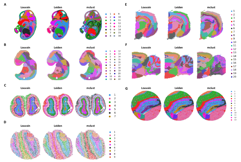
Figure S14: Comparison analysis between Leiden, Louvain, and mclust with the output of MuST as input. Visualization of clustering results from Louvain, Leiden, and mclust on Stereo-seq E14.5 mouse embryo data (A), Stereo-seq 9.5 mouse embryo data (B), Stereo-seq mouse olfactory bulb tissue sections (C), Slide-seqV2 mouse olfactory bulb tissue sections (D), 10x Visium coronal mouse brain section (E), 10x Visium mouse sagittal posterior brain section (F), and SlideseqV2 mouse hippocampus data (G).

In MuST, we chose mclust as the default clustering method because our assessment shows that mclust performs better than Leiden and Louvain in most cases. Here, we compare the clustering results on different datasets using Leiden, Louvain, and mclust shown in Fig. S14. mclust consistently outperforms Leiden and Louvain on all datastes. Visually, the clusters identified by mclust are more continuous. Nevertheless, we also include Leiden and Louvain in MuST as alternative clustering methods.

Appendix C Supplementary Tables

Table S1. Description of all ST datasets used in this study.
Table S2. Hyperparameters of MuST in all ST datasets.
Table S3. Marker gene selection of MuST on mouse embryo at E14.5 dataset acquired with Stereo-seq.
Table S4. Marker gene selection of MuST on mouse embryo at E9.5 dataset acquired with Stereo-seq.
Table S5. Marker gene selection of MuST on mouse hippocampus dataset acquired with Slide-seqV2.
Table S6. Marker gene selection of MuST on coronal mouse brain section acquired with 10x Visium.
Table S7. Marker gene selection of MuST on mouse sagittal posterior brain section acquired with 10x Visium.
Table S8. Marker gene selection of MuST on coronal mouse olfactory bulb tissue dataset acquired with Stereo-seq.
Table S9. Marker gene selection of MuST on coronal mouse olfactory bulb tissue dataset acquired with Slide-seqV2.
Table S10. Marker gene selection of MuST on slice 151673 of DLPFC dataset acquired with 10x Visium.

Appendix D Supplementary Figures

Figure S1. MuST alleviates the modality bias phenomenon in mouse brain data. A H&E image of mouse brain coronal section and mouse sagittal posterior brain section. B Contribution of the morphology (Mor.) modality, transcriptome (Tra.) modality and spatial (Spa.) modality input data or MuST embedding to data labeling. C Contribution visualization of the Mor. modality, Tra. modality and Spa. modality input data or MuST embedding to data labeling.
Figure S2. MuST alleviates the modality bias phenomenon in mouse embryo data. A Contribution of the morphology (Mor.) modality, transcriptome (Tra.) modality and spatial (Spa.) modality input data or MuST embedding to data labeling on mouse embryo 14.5 and 9.5 datasets. C Contribution visualization of the Mor. modality, Tra. modality and Spa. modality input data or MuST embedding to data labeling.
Figure S3. MuST enables accurate identification of different organs in the Stereo-seq mouse embryo. A Tissue domain annotations of the E14.5 mouse embryo data obtained from the original Stereo-seq study. B Clustering results by GraphST and MuST on the E14.5 mouse embryo. C Cluster visualization of selected spatial domains identified by the original Stereo-seq study, MuST and GraphST, respectively.
Figure S4. MuST enables accurate identification of different organs in the Stereo-seq mouse embryo. A Tissue domain annotations of the E9.5 mouse embryo data obtained from the original Stereo-seq study. B Clustering results by GraphST and MuST on the E9.5 mouse embryo. C Cluster visualization of selected spatial domains identified by the original Stereo-seq study, MuST and GraphST, respectively.
Figure S5. Spatial deconvolution of MuST’s results in adult mouse brain section profiled by 10x Visium. A Allen Brain Institute reference atlas diagram and H&E image of the mouse cortex. B Allen Brain Institute reference atlas diagram and H&E image of the mouse sagittal. C Spatial deconvolution of the identified domains by MuST on coronal mouse brain section. D Spatial deconvolution of the identified domains by MuST on mouse sagittal posterior brain section. E Spatial deconvolution of the coronal mouse brain section. F Spatial deconvolution of the mouse sagittal posterior brain section.
Figure S6. Embedding analysis of MuST on the mouse olfactory bulb tissue and mouse embryo. A Mean relative rank error (MRRE) scores and UMAP visualizations generated by SpcGCN, MUSE, DeepST, GraphST and MuST representations on the Stereo-seq E14.5 mouse embryo data. Among them, methods MUSE and DeepST have an out of memory (OOM) problem. B MRRE scores and UMAP visualizations generated by the representations of five methods on the Stereo-seq E9.5 mouse embryo data. C MRRE scores, UMAP visualizations and PAGA graphs generated by the representations of five methods on the Stereo-seq mouse olfactory bulb tissue section. D MRRE scores, spot visualizations and PAGA graphs generated by the representations of five methods on the Slide-seqv2 mouse olfactory bulb tissue section.
Figure S7. Manual annotations and comparison of spatial domains identified by stSME, SpaGCN, MUSE, DeepST, GraphST and MuST on the 12 slices of DLPFC dataset.
Figure S8. Marker genes selection for each anatomical region of mouse hippocampus data acquired with SlideseqV2.
Figure S9. Marker genes selection for each region of coronal mouse brain section acquired with 10x Visium.
Figure S10. Marker genes selection for each region of mouse sagittal posterior brain section acquired with 10x Visium.
Figure S11. Marker genes selection for each laminar organization of coronal mouse olfactory bulb tissue datasets acquired with Slide-seqV2.
Figure S12. Marker genes selection for each laminar organization of coronal mouse olfactory bulb tissue datasets acquired with Stereo-seq.
Figure S13. Comparison analysis between Leiden, Louvain, and mclust with the output of MuST as input. Visualization of clustering results from Louvain, Leiden, and mclust on Stereo-seq E14.5 mouse embryo data (A), Stereo-seq 9.5 mouse embryo data (B), Stereo-seq mouse olfactory bulb tissue sections (C), Slide-seqV2 mouse olfactory bulb tissue sections (D), 10x Visium coronal mouse brain section (E), 10x Visium mouse sagittal posterior brain section (F), and SlideseqV2 mouse hippocampus data (G).

Table S1: Description of all ST datasets used in this study.

Platform	Tissue	Section	#Spots/bins	#Genes	Related figures	Reference
Stereo-Seq	Mouse embyro	E14.5	92928	18582	Fig. 2, Fig. C1, Fig. C4, Fig. C11, Tab. C3	[10]
		E9.5	5913	25568	Fig. 2, Fig. C2, Fig. C4, Fig. C11, Tab. C4	[10]
	Mouse olfactory bulb	MOB	19109	27106	Fig. 5, Fig. C4, Fig. C9, Fig. C11, Tab. C8	[10]
Slide-SeqV2	Mouse hippocampus	Puck_200115_08	53172	23264	Fig. 3, Fig. C6, Fig. C11, Tab. C5	[8]
	Mouse olfactory bulb	Puck_200127_15	20139	21220	Fig. 5, Fig. C4, Fig. C10, Fig. C11, Tab. C9	[8]
10x Visium	Mouse brain	Mouse Brain Section (Coronal)	2702	32285	Fig. 4, Fig. C3, Fig. C7, Fig. C11, Tab. C6	[49]
	Mouse brain	Mouse Brain Section (Sagittal-Posterior)	3355	32285	Fig. 4, Fig. C3, Fig. C8, Fig. C11, Tab. C7
	Human dorsolateral prefrontal cortex (DLPFC)	151507	4220	33538	Fig. 6, Fig. C5	[41]
		151508	4381	33538	Fig. 6, Fig. C5	[41]
		151509	4788	33538	Fig. 6, Fig. C5	[41]
		151510	4595	33538	Fig. 6, Fig. C5	[41]
		151669	3636	33538	Fig. 6, Fig. C5	[41]
		151670	3484	33538	Fig. 6, Fig. C5	[41]
		151671	4093	33538	Fig. 6, Fig. C5	[41]
		151672	3888	33538	Fig. 6, Fig. C5	[41]
		151673	3611	33538	Fig. 6, Fig. C5, Tab. C10	[41]
		151674	3635	33538	Fig. 6, Fig. C5	[41]
		151675	3566	33538	Fig. 6, Fig. C5	[41]
		151676	3431	33538	Fig. 6, Fig. C5	[41]

Table S2: Hyperparameters of MuST in all ST datasets.

Section	$K^{mo}$	$K^{tr}$	$r^{mo}_{u}$	$r^{tr}_{u}$	$\nu$	$d_{emb}$	$\theta$	$\lambda$
ME95	5	9	0.1	1	0.05	72	1	0.015
ME145	5	7	0.1	1	0.05	72	1	0.0015
MOB	10	10	0.1	0.1	0.01	64	1	0.001
DLPFC	3	11	1	0.3	0.13	72	0.9	0.12
Mouse Brain Section (Coronal)	7	7	0.1	0.1	0.05	72	0.9	0.01
Mouse Brain Section (Sagittal-Posterior)	5	9	1	0.1	0.15	72	0.7	0.001
Puck_200115_08	5	25	0.1	0.5	1	72	1	0.005
Puck_200127_15	10	50	0.1	0.5	0.005	100	1	0.00015

Table S3: Marker gene selection of MuST on mouse embryo at E14.5 dataset acquired with Stereo-seq.

Clusters	Marker genes
C1	Afp, Hbb-bs, Tuba1a, Ttn, Hbb-bt, Apoa2, Mt1, H19, Col3a1, Col1a2, Lgals1, Fabp7
C2	Tuba1a, Fabp7, H19, Col3a1, Hbb-bs, Lgals1, Col1a2, Afp, Stmn2, Hbb-bt, Rtn1, Dbi
C3	Col3a1, Tuba1a, Col1a2, Ttn, Hbb-bs, Afp, Myh3, Gphn, Mt1, Hbb-bt, Krt5, Col1a1
C4	Afp, Apoa2, Slc25a37, Hbb-bt, Gpx1, Alb, Mt1, Apoa1, Hba-a2, Mt2, Col3a1, Hba-a1
C5	Krt5, Tuba1a, Krt15, Mt1, Hbb-bs, Afp, Col3a1, H19, Hbb-bt, Lgals1, Col1a2, Fabp7
C6	Ttn, Myh3, Neb, Hbb-bs, Tceal7, Actc1, Myl1, Nrk, Tnni2, Hba-a1, Col3a1, Acta1
C7	Ugt2a2, H19, Tuba1a, Col3a1, Sult1e1, Lgals1, Hbb-bs, Afp, Hbb-bt, Col1a2, Fabp7, Igf2
C8	Krt5, Cxcl14, Tuba1a, Afp, Perp, Col3a1, Anxa2, Hbb-bs, H19, S100a6, Krt15, Col1a2
C9	Col11a1, Col2a1, Tuba1a, Gphn, Hbb-bs, Col3a1, Afp, Malat1, H19, Hbb-bt, Mt1, Col1a2
C10	Fabp7, Tuba1a, Slc1a3, Dbi, Hbb-bs, Mylpf, Tubb2b, Spon1, H19, Fez1, Camk1d, Afp
C11	Trps1, Alx1, Mt1, Hbb-bs, Hpse2, Tuba1a, Col2a1, Camk1d, Malat1, Msx1, Col3a1, Afp
C12	Myh11, Acta2, Mylk, Tuba1a, Actg2, Hbb-bs, Hba-a1, Afp, Prkg1, H19, Col3a1, Fabp7
C13	Tuba1a, Map1b, Tmsb10, Col1a2, Col3a1, Hbb-bs, Nnat, Rtn1, H19, Camk1d, Afp, Lgals1
C14	Neurod6, Tuba1a, H19, Hbb-bs, Lgals1, Fabp7, Pantr1, Hbb-bt, Actc1, Nfib, Col3a1, Igf2
C15	Tuba1a, Rtn1, Hbb-bs, Stmn2, Map1b, H19, Gphn, Gap43, Tubb2a, Tmsb10, Lgals1, Afp
C16	Nppa, Myh6, Tuba1a, Tnnt2, Tnni3, H19, Hbb-bs, Afp, Hbb-bt, Actc1, Col3a1, Myl7

Table S4: Marker gene selection of MuST on mouse embryo at E9.5 dataset acquired with Stereo-seq.

Clusters	Marker genes
C1	Postn, Fabp7, Igf2, Hbb-bs, H19, Pantr1, Msx1, Gata6, Sox2, Ckb, Hbb-y, Igfbp2
C2	Fabp7, Igf2, Hbb-y, Hbb-bh1, Hoxb3os, Ckb, Pantr1, Col3a1, H19, Tmsb4x, Otx2, Cnn2
C3	Myl7, Actc1, Acta1, Tnni1, Myl4, Igf2, Fabp7, Tnnt2, Myh7, Hbb-y, Marcks, Lars2
C4	Fabp7, Igf2, Hbb-bh1, Ckb, H19, Hbb-y, Dlk1, Col3a1, Tmsb4x, Crabp1, Rfx4, Tuba1a
C5	Igf2, Fabp7, Myl7, Ckb, Zic1, Mest, H19, Crabp1, Foxf1, Peg3, Hbb-y, Actc1
C6	Fabp7, Igf2, Ckb, Hbb-bh1, H19, Hbb-y, Cnn2, Pantr1, Col3a1, Rfx4, Sox2, Vim
C7	Lars2, Fabp7, Marcks, Igf2, Cnn2, Flrt2, Zc3h7a, Ckb, Ebf1, Gm26561, Sulf1, Acta1
C8	Meox1, Myl7, Fabp7, Igf2, Msx1, Dmrt2, Mylpf, Acta1, Lars2, Actc1, Zc3h7a, Pantr1
C9	Fabp7, Igf2, Pantr1, Sox2, Id4, Hbb-y, Ckb, Rfx4, H19, Dlk1, Col3a1, Cnn2
C10	Fabp7, Igf2, Vim, Ckb, Hbb-y, Pantr1, Rfx4, Sox2, H19, Msi1, Lars2, Marcks
C11	Cpox, Hbb-bt, Fabp7, Mt2, Igf2, H19, Hba-a2, Mt1, Hbb-y, Sox2, Abcb10, Pantr1
C12	Fabp7, Igf2, Hbb-y, Ckb, H19, Crabp1, Pantr1, Zic1, Hbb-bh1, Sox2, Myl7, Vim
C13	Mylpf, Fabp7, Igf2, Pantr1, Hba-x, Hbb-bh1, Vim, Myl7, Meox2, Ckb, H19, Nnat
C14	Igf2, Fabp7, Ckb, Hbb-bh1, Hbb-y, H19, Ntn1, Msx1, Tmsb4x, Mest, Nkx6-1, Col3a1
C15	Fabp7, Igf2, Msx1, H19, Pantr1, Acta1, Hand2, Rfx4, Actc1, Tnni1, Dlk1, Myl7
C16	Hbb-y, Fabp7, Igf2, Sox2, H19, Gm42418, Ckb, Pantr1, Bpgm, Mt2, Cenpa, Ldha
C17	Fabp7, Igf2, H19, Myl7, Hbb-bs, Ckb, Pantr1, Dlk1, Sox2, Postn, Mest, Hoxc9
C18	Pax1, Fabp7, Arg1, Meox2, Vim, Igf2, Ckb, Sox2, Myl7, Pantr1, H19, Vcan
C19	Fabp7, Igf2, Ebf1, Pantr1, Ckb, Stmn2, Hbb-y, H19, Hbb-bh1, Lars2, Nefm, Vim
C20	Afp, Fabp7, Igf2, Pantr1, Ckb, H19, Myl7, Hbb-y, Sox2, Lars2, Actc1, Vim
C21	Fabp7, Hbb-bh1, Igf2, Hbb-y, Hoxb3os, Col3a1, Pantr1, Ckb, Tmsb4x, H19, Crabp1, Lars2
C22	Igf2, Fabp7, Ckb, Hbb-y, H19, Ntn1, Hbb-bh1, Col3a1, Rfx4, Cnn2, Pantr1, Tmsb4x

Table S5: Marker gene selection of MuST on mouse hippocampus dataset acquired with Slide-seqV2.

Clusters	Marker genes
C1	Plp1, Pcp4, Snap25, Mbp, Meg3, Nrgn, Hpca, Ncald, Mef2c, Mobp, Ttr, Ppp3ca
C2	Pcp4, Hpca, Nrgn, Plp1, Rora, Pcp4l1, Mbp, Ccdc136, Cit, Ttr, Tcf7l2, Tnnt1
C3	Nrgn, Snap25, Mef2c, Pcp4, Ncald, Hpca, Plp1, Meg3, Lamp5, Pde1a, 3110035E14Rik, Lmo4
C4	Plp1, Mbp, Pcp4, Mobp, Hpca, Qdpr, Mal, Cnp, Cldn11, Nrgn, Sept4, Ptgds
C5 (CA1)	Hpca, Ppp3ca, Nrgn, Itpka, Wipf3, Prkcb, Plp1, Tmsb4x, Pcp4, Cck, Meg3, Mbp
C6 (CA3)	Hpca, Cpne6, Ppp3ca, Cplx2, Snap25, Plp1, Chgb, Hs3st4, Nrgn, Pcp4, Calm2, Tmsb4x
C7 (Dentate Gyrus)	Hpca, Ppp3ca, Ncdn, Nrgn, Plp1, Cplx2, Snap25, Pcp4, Olfm1, Mbp, Itpka, Meg3
C8 (Interneuron)	Gad1, Sst, Pcp4, Plp1, Hpca, Mbp, Gad2, Nrgn, Cnr1, Snap25, Meg3, Ncald
C9	Meg3, Nrgn, Snhg11, Pcp4, Snap25, Hpca, Plp1, Malat1, Calb2, Ptk2b, Mef2c, Tmsb4x
C10 (LH)	Pcp4, Nrgn, Hpca, Plp1, Ptgds, Nwd2, Snap25, Nnat, Nefm, Ttr, Gap43, Meg3
C11 (V3)	Ttr, Nrgn, Pcp4, Plp1, 1500015O10Rik, Hpca, Zic1, Pcp4l1, Malat1, Mbp, Meg3, Enpp2
C12 (MH)	Nwd2, Zic1, Ttr, Hpca, Calb2, Pcp4, Tac2, Cd63, Plp1, Tcf7l2, Meg3, Gng8
C13	Apod, Ptgds, Aqp4, Agt, Pcp4, Vim, Hpca, Plp1, Nrgn, Zic1, Nwd2, Ttr

Table S6: Marker gene selection of MuST on coronal mouse brain section acquired with 10x Visium.

Clusters	Marker genes
C1	Tcf7l2, Nrgn, Sparc, Ddn, Ctxn3, Camk2n1, Slc17a6, Slc17a7, Hlf, Ctxn1, Rims3, Adarb1
C2	Nrgn, Mobp, Tcf7l2, Slc17a7, Mbp, Pvalb, Sparc, Prkcd, Vxn, Camk2n1, Fxyd7, Ddn
C3	Hap1, Baiap3, Pmch, 6330403K07Rik, Slc17a7, Nrgn, Camk2n1, Resp18, Nsmf, Tcf7l2, Ddn, Cartpt
C4 (V3)	Slc17a7, Mia, Ncdn, Thy1, Camk2n1, Hap1, Cck, Mbp, Nrgn, Baiap3, Tcf7l2, Nsmf
C5	Ddn, Ttr, Camk2n1, Fth1, Hpca, Nrgn, Slc17a7, Mbp, Spink8, Pantr1, Cabp7, Ctxn1
C6 (Dentate Gyrus)	Camk2n1, Slc17a7, Nrgn, Vxn, Tcf7l2, Eef1a1, Pcp4, Ddn, Hpca, Nsmf, Mbp, Adcy1
C7	Syn2, Camk2n1, Nptxr, C1ql3, Nr2f2, Vxn, Ddn, Nnat, Uchl1, Nrgn, Lypd1, Pcp4
C8	Prkcd, Adarb1, Tcf7l2, Nrgn, Ctxn1, Rora, Tnnt1, Pcp4, Atp2b1, Slc17a7, Ptpn3, Mobp
C9 (Cerebral cortex 2)	Camk2n1, Nrgn, Mef2c, Snap25, Dkkl1, Mbp, Plcxd2, Slc17a7, Atp1a1, Pcp4, Ddn, Vxn
C10	Camk2n1, Ddn, Slc17a7, Mbp, Penk, Hpcal4, Hpcal1, Hpca, Fth1, Syn2, Ctxn1, Vxn
C11	Slc17a7, Nrgn, Tcf7l2, Camk2n1, Sparc, Ddn, Baiap3, Nnat, Rpl17, Hap1, Tmsb4x, Thy1
C12	Camk2n1, Ddn, Mbp, Olfm1, Hpca, Nrgn, Slc17a7, Nptxr, Penk, Ctxn1, Hpcal4, Vxn
C13	Penk, Slc17a7, Camk2n1, Ctxn1, Arpp21, Hpcal4, Nrgn, Ddn, Tcf7l2, Mbp, Wfs1, Eef1a1
C14 (Cerebral cortex 1)	Camk2n1, Mbp, Pcp4, Nrgn, Lamp5, Tubb2a, Cplx2, Tmsb10, Ddn, Atp1a1, Slc17a7, Vxn
C15 (Cerebral cortex 3)	Camk2n1, Slc17a7, Vxn, Eef1a1, Ddn, Tcf7l2, Mbp, Nrgn, 1110008P14Rik, Fth1, Nptxr, Ttr
C16 (Fiber tracts)	Mbp, Fth1, Mobp, Thy1, Ncdn, Camk2n1, Tcf7l2, Nrgn, Tmsb4x, Slc17a7, Snap25, Cnp
C17	Prkcd, Adarb1, Tcf7l2, Rora, Atp2b1, Pcp4, Nrgn, Tnnt1, Camk2n1, Ctxn1, Slc17a7, Ptpn3
C18 (CA1)	Hpca, Camk2n1, Nrgn, Tmsb4x, Wipf3, Slc17a7, Vxn, Spink8, Tcf7l2, Ddn, Mbp, Ppp3ca
C19 (Cerebral cortex 4)	Vxn, Tmsb4x, Slc17a7, Camk2n1, Mbp, Diras2, Ttc9b, Mobp, Nr4a2, Nptxr, Ncald, Nrgn
C20 (CA3)	Camk2n1, Slc17a7, Tcf7l2, Nrgn, Vxn, Hpca, Ctxn1, Mbp, Ddn, Fth1, Hpcal4, Cnih2

Table S7: Marker gene selection of MuST on the mouse sagittal posterior brain section acquired with 10x Visium.

Clusters	Marker genes
C1 (CA1)	Mbp, Pcp2, Camk2a, Nrgn, Hpca, Ddn, Rasgrp1, Cck, Nnat, Stmn1, Pvalb, Ctxn1
C2	Nrgn, Mbp, Ddn, Camk2a, Pcp4, Slc1a2, Pvalb, Ctxn1, Pcp2, Plp1, Pantr1, Snap25
C3	Mbp, Camk2a, Cpe, Rasgrp1, Plp1, Atp1a1, Nnat, Ctxn1, Slc17a7, Snap25, Nrgn, Cck
C4	Nnat, Ccn3, Ly6h, Mbp, Dcn, Crym, Nptxr, Ctxn1, Ttr, Ddn, Trh, Pcp2
C5 (Coronal structure)	Atp1a1, Camk2a, Grin2c, Nrep, Adcy1, Mbp, Pcp2, Cbln3, Pvalb, Cbln1, Gabra6, Nrgn
C6 (Fiber tracts)	Mbp, Plp1, Nrgn, Cpe, Cck, Atp1a1, Camk2a, Trf, Mobp, Pcp2, Camkv, Ctxn1
C7 (Cerebral cortex 2)	Pcp2, Mbp, Nrgn, Atp1a1, Camk2n1, Pcp4, Camk2a, Slc1a2, 1110008P14Rik, Nnat, Dkk3, Ddn
C8	Mbp, Cpe, Pvalb, Nefl, Mobp, Snap25, Pcp2, Vamp1, Camk2a, Nrgn, Cck, Hoxb5
C9 (Dentate Gyrus)	Mbp, Pcp2, Ddn, Camk2a, Olfm1, Pvalb, Nrgn, Synpr, Snhg11, Ctxn1, Ncdn, Pcp4
C10 (Thin layer 1)	Pcp2, Mbp, Pvalb, Atp1a1, Itpr1, Gng13, Camk2a, Mobp, Stmn1, Cbln1, Car8, Cbln3
C11 (Thin layer 2)	Pcp2, Mbp, Nptx1, Pvalb, Nrgn, Cbln1, Calm2, Ppp1r17, Car8, Gabra6, Camk2a, Pcp4
C12 (Thin layer 3)	Pcp2, Mbp, Cbln1, Pvalb, Atp1a1, Mobp, Camk2a, Nptx1, Car8, Gabra6, Cbln3, Calm2
C13 (Cervical)	Hoxb5, Mbp, Pcp2, Cck, Pvalb, Camk2a, Slc6a5, Nefm, Vamp1, Nrgn, Zwint, Vsnl1
C14	Mbp, Camk2n1, Camk2a, Mef2c, Nnat, Cck, Ctxn1, Pcp2, Lypd1, Stx1a, Atp1a1, Snhg11
C15 (Cerebral cortex 1)	Prkcd, Tnnt1, Cck, Pcp2, Rasgrp1, Ntng1, Mbp, Rgs16, Tcf7l2, Pdp1, Nrgn, Ndrg4
C16	Ddn, Pvalb, Camk2a, Mbp, Nrgn, Vsnl1, C1ql2, Uchl1, Atp1a1, Pcp2, Ctxn1, Stmn1
C17	Mbp, Pcp2, Nrgn, Camk2a, Pvalb, Igfbp2, Nnat, Ddn, Cck, Ctxn1, Atp1a1, Ccn3
C18	Mbp, Nptxr, Trh, Pcp2, Nrgn, Ctxn1, Nnat, Camk2a, Ccn3, Lypd1, Hap1, Ddn
C19	Lypd1, Ctxn1, Pgrmc1, Mbp, Nnat, Ccn3, Ttr, Nr2f2, Pcp2, Ptgds, Ly6h, Trh
C20 (CA3)	Crym, Hpca, Pvalb, Mbp, Camk2a, Nrgn, Cpne6, Ccn3, Pcp2, Ctxn1, Ak5, Cnih2

Table S8: Marker gene selection of MuST on coronal mouse olfactory bulb tissue dataset acquired with Stereo-seq.

Clusters	Marker genes
ONL	Pcp4, Gad1, Gng13, Fabp7, Ptn, S100a5, Calb2, Nrxn3, Apoe, Kcnb2, Ptgds, Ptprd
EPL	Calb2, Nrsn1, Pcp4, Nxph1, Nrxn3, Apoe, Gng13, Fabp7, Ptn, S100a5, Cck, Zic1
GCL	Gad1, Pcp4, Pcp4l1, Nme7, Ncdn, Ptprd, Stxbp6, Spp1, Gabra1, Atp1b1, Prkca
IPL	Spp1, Stmn2, Uchl1, Gad1, Gabra1, Pcp4, Cpe, Lhfpl3, Nmb, Nef, Ptprd, Cplx1
MCL	Gad1, Pcp4, Nrxn3, Kcnb2, Ppp3ca, Atp1a2, Plp1, Calb2, Nme7, Pbx3, Tenm3, Cpne4
GL	Gng13, Ptn, Fabp7, Ptgds, S100a5, Apoe, Atp1a2, Npy, Plp1, Gad1, Pcp4, Snap25
RMS	Plp1, Pcp4, Nrep, Gad1, Nme7, Nrxn3, Pbx3, Mobp, Ptgds, Apoe, Tenm3, Calb2

• Here we assign clusters to the corresponding tissue structure: olfactory nerve layer (ONL), external plexiform layer (EPL), granule cell layer (GCL), internal plexiform layer (IPL), mitral cell layer (MCL), glomerular layer (GL), and rostral migratory stream (RMS) according to the ground truth.

Table S9: Marker gene selection of MuST on coronal mouse olfactory bulb tissue dataset acquired with Slide-seqV2.

Clusters	Marker genes
GCL	Pcp4, Nrxn3, Camk2b, Doc2g, Meis2, Ppp3ca, Nrsn1, S100a5, Cck, Fabp7, Atp1a2, Dlg2
EPL	Pcp4, S100a5, Nrxn3, Doc2g, Camk2b, Fabp7, Apod, Cck, Atp1a2, Ppp3ca, Meis2, Nrsn1
MCL	Doc2g, Cck, Rab3b, Pcp4, Olfm1, S100a5, Nrsn1, Map1b, Cdhr1, Slc17a7, Fabp7, Nrxn3
ONL	S100a5, Fabp7, Apod, Pcp4, Ptgds, Ptn, Gng13, Gad1, Nrsn1, Omp, Doc2g, Plp1
RMS	Pcp4, Mbp, Nrxn3, Doc2g, Nrgn, S100a5, Tubb2b, Camk2b, Meis2, Nrsn1, Nrep, Mobp
GL	S100a5, Nrsn1, Pcp4, Fabp7, Apod, Calb2, Gng13, Ptgds, Cck, Nrxn3, Doc2g, Vsnl1
IPL	Pcp4, Atp1b1, Nrxn3, Doc2g, Nrsn1, Camk2b, Ppp3ca, Gad1, Scg2, Cck, Rab3b, Fxyd6
AOBgr	Nrxn3, Cpne6, Pcp4, Tac1, Doc2g, Fxyd6, Calb2, Plcb1, Camk2b, Dpp6, Jph4, Atp2b4
AOB	Fxyd6, Slc17a7, Rab3b, Pcp4, Stmn2, Uchl1, Doc2g, Cdhr1, Calb2, Cck, Nrxn3, Ptprd

• Here we assign clusters to the corresponding tissue structure: granule cell layer (GCL), external plexiform layer (EPL), mitral cell layer (MCL), olfactory nerve layer (ONL), rostral migratory stream (RMS), glomerular layer (GL), internal plexiform layer (IPL), granular layer of the accessory olfactory bulb (AOBgr) and accessory olfactory bulb (AOB) according to the ground truth.

Table S10: Marker gene selection of MuST on slice 151673 of DLPFC dataset acquired with 10x Visium.

Clusters	Marker genes
White Matter	MBP, PLP1, GFAP, CNP, PTGDS, TF, SNAP25, CRYAB, TMSB10, MOBP
Layer 1	MBP, GFAP, SNAP25, PLP1, MALAT1, TUBA1B, NEFL, CAMK2N1, STMN2, SLC24A2
Layer 2	MBP, CAMK2N1, TUBA1B, HPCAL1, NEFL, MALAT1, PLP1, TMSB10, ENC1, SOWAHA
Layer 3	MBP, PLP1, TMSB10, DIRAS2, GFAP, CAMK2N1, TUBA1B, NEFL, SNAP25, MALAT1
Layer 4	MBP, PLP1, TUBA1B, IGKC, IGLC2, GFAP, SNAP25, TMSB10, MALAT1, SCGB1D2
Layer 5	MBP, TMSB10, PCP4, PLP1, SNAP25, GFAP, TUBA1B, DIRAS2, HPCAL1, MALAT1
Layer 6	MBP, PLP1, DIRAS2, GFAP, PCP4, TMSB10, KRT17, SNCG, B3GALT2, SNAP25

References

- \bibcommenthead
- [1] Kolodziejczyk, A. A., Kim, J. K., Svensson, V., Marioni, J. C. & Teichmann, S. A. The technology and biology of single-cell rna sequencing. Molecular cell 58, 610–620 (2015).
- [2] Saliba, A.-E., Westermann, A. J., Gorski, S. A. & Vogel, J. Single-cell rna-seq: advances and future challenges. Nucleic acids research 42, 8845–8860 (2014).
- [3] Luecken, M. D. & Theis, F. J. Current best practices in single-cell rna-seq analysis: a tutorial. Molecular systems biology 15, e8746 (2019).
- [4] Erhard, F. et al. Time-resolved single-cell rna-seq using metabolic rna labelling. Nature Reviews Methods Primers 2, 77 (2022).
- [5] Satija, R., Farrell, J. A., Gennert, D., Schier, A. F. & Regev, A. Spatial reconstruction of single-cell gene expression data. Nature biotechnology 33, 495–502 (2015).
- [6] Williams, C. G., Lee, H. J., Asatsuma, T., Vento-Tormo, R. & Haque, A. An introduction to spatial transcriptomics for biomedical research. Genome Medicine 14, 1–18 (2022).
- [7] Hudson, W. H. & Sudmeier, L. J. Localization of t cell clonotypes using the visium spatial transcriptomics platform. STAR protocols 3, 101391 (2022).
- [8] Rodriques, S. G. et al. Slide-seq: A scalable technology for measuring genome-wide expression at high spatial resolution. Science 363, 1463–1467 (2019).
- [9] Stickels, R. R. et al. Highly sensitive spatial transcriptomics at near-cellular resolution with slide-seqv2. Nature biotechnology 39, 313–319 (2021).
- [10] Chen, A. et al. Spatiotemporal transcriptomic atlas of mouse organogenesis using dna nanoball-patterned arrays. Cell 185, 1777–1792 (2022).
- [11] Ståhl, P. L. et al. Visualization and analysis of gene expression in tissue sections by spatial transcriptomics. Science 353, 78–82 (2016).
- [12] Longo, S. K., Guo, M. G., Ji, A. L. & Khavari, P. A. Integrating single-cell and spatial transcriptomics to elucidate intercellular tissue dynamics. Nature Reviews Genetics 22, 627–644 (2021).
- [13] Rao, A., Barkley, D., França, G. S. & Yanai, I. Exploring tissue architecture using spatial transcriptomics. Nature 596, 211–220 (2021).
- [14] Tian, L., Chen, F. & Macosko, E. Z. The expanding vistas of spatial transcriptomics. Nature Biotechnology 41, 773–782 (2023).
- [15] Long, Y. et al. Spatially informed clustering, integration, and deconvolution of spatial transcriptomics with graphst. Nature Communications 14, 1155 (2023).
- [16] Bao, F. et al. Integrative spatial analysis of cell morphologies and transcriptional states with muse. Nature biotechnology 40, 1200–1209 (2022).
- [17] Dries, R. et al. Giotto, a pipeline for integrative analysis and visualization of single-cell spatial transcriptomic data. BioRxiv 701680 (2019).
- [18] Xu, Y. et al. Structure-preserving visualization for single-cell rna-seq profiles using deep manifold transformation with batch-correction. Communications Biology 6, 369 (2023).
- [19] Kleshchevnikov, V. et al. Cell2location maps fine-grained cell types in spatial transcriptomics. Nature biotechnology 40, 661–671 (2022).
- [20] Ma, Y. & Zhou, X. Spatially informed cell-type deconvolution for spatial transcriptomics. Nature biotechnology 40, 1349–1359 (2022).
- [21] Dumitrascu, B., Villar, S., Mixon, D. G. & Engelhardt, B. E. Optimal marker gene selection for cell type discrimination in single cell analyses. Nature communications 12, 1186 (2021).
- [22] Wolf, F. A. et al. Paga: graph abstraction reconciles clustering with trajectory inference through a topology preserving map of single cells. Genome biology 20, 1–9 (2019).
- [23] Gat, I., Schwartz, I., Schwing, A. & Hazan, T. Removing bias in multi-modal classifiers: Regularization by maximizing functional entropies. Advances in Neural Information Processing Systems 33, 3197–3208 (2020).
- [24] Guo, Y. et al. On modality bias recognition and reduction. ACM Transactions on Multimedia Computing, Communications and Applications 19, 1–22 (2023).
- [25] Dong, K. & Zhang, S. Deciphering spatial domains from spatially resolved transcriptomics with an adaptive graph attention auto-encoder. Nature communications 13, 1739 (2022).
- [26] Ren, H., Walker, B. L., Cang, Z. & Nie, Q. Identifying multicellular spatiotemporal organization of cells with spaceflow. Nature communications 13, 4076 (2022).
- [27] Zong, Y. et al. const: an interpretable multi-modal contrastive learning framework for spatial transcriptomics. bioRxiv 2022–01 (2022).
- [28] Zeng, Y. et al. Identifying spatial domain by adapting transcriptomics with histology through contrastive learning. Briefings in Bioinformatics 24, bbad048 (2023).
- [29] Li, J., Chen, S., Pan, X., Yuan, Y. & Shen, H.-B. Cell clustering for spatial transcriptomics data with graph neural networks. Nature Computational Science 2, 399–408 (2022).
- [30] Teng, H., Yuan, Y. & Bar-Joseph, Z. Clustering spatial transcriptomics data. Bioinformatics 38, 997–1004 (2022).
- [31] Hu, J. et al. Spagcn: Integrating gene expression, spatial location and histology to identify spatial domains and spatially variable genes by graph convolutional network. Nature methods 18, 1342–1351 (2021).
- [32] Pham, D. et al. stlearn: integrating spatial location, tissue morphology and gene expression to find cell types, cell-cell interactions and spatial trajectories within undissociated tissues. BioRxiv 2020–05 (2020).
- [33] Zhang, X., Wang, X., Shivashankar, G. & Uhler, C. Graph-based autoencoder integrates spatial transcriptomics with chromatin images and identifies joint biomarkers for alzheimer’s disease. Nature Communications 13, 7480 (2022).
- [34] Xu, C. et al. Deepst: identifying spatial domains in spatial transcriptomics by deep learning. Nucleic Acids Research 50, e131–e131 (2022).
- [35] Bergenstråhle, L. et al. Super-resolved spatial transcriptomics by deep data fusion. Nature biotechnology 40, 476–479 (2022).
- [36] Zang, Z. et al. Deep manifold embedding of attributed graphs. Neurocomputing 514, 83–93 (2022).
- [37] Zang, Z. et al. Dlme: Deep local-flatness manifold embedding. European Conference on Computer Vision 576–592 (2022).
- [38] Kipf, T. N. & Welling, M. Semi-supervised classification with graph convolutional networks (2017). 1609.02907.
- [39] Mamoor, S. The alpha subunit of the gamma-aminobutyric acid receptor, gabra1, is differentially expressed in the brains of patients with schizophrenia. OSF Preprints https://doi.org/10.31219/osf.io/m93ya (2020).
- [40] Zhang, Y. et al. Association between nrgn gene polymorphism and resting-state hippocampal functional connectivity in schizophrenia. BMC psychiatry 19, 1–9 (2019).
- [41] Maynard, K. R. et al. Transcriptome-scale spatial gene expression in the human dorsolateral prefrontal cortex. Nature neuroscience 24, 425–436 (2021).
- [42] Winter, E. The shapley value. Handbook of game theory with economic applications 3, 2025–2054 (2002).
- [43] Roth, A. E. The Shapley value: essays in honor of Lloyd S. Shapley (Cambridge University Press, 1988).
- [44] Scrucca, L., Fop, M., Murphy, T. B. & Raftery, A. E. mclust 5: clustering, classification and density estimation using gaussian finite mixture models. The R journal 8, 289 (2016).
- [45] Zang, Z. et al. Evnet: An explainable deep network for dimension reduction. IEEE Transactions on Visualization and Computer Graphics (2022).
- [46] Becht, E. et al. Dimensionality reduction for visualizing single-cell data using umap. Nature biotechnology 37, 38–44 (2019).
- [47] Saltelli, A. Sensitivity analysis for importance assessment. Risk analysis 22, 579–590 (2002).
- [48] Zou, H. The adaptive lasso and its oracle properties. Journal of the American statistical association 101, 1418–1429 (2006).
- [49] 10xgenomics. 10x genomics. https://www.10xgenomics.com/resources/datasets/ (2023).
- [50] Sunkin, S. M. et al. Allen brain atlas: an integrated spatio-temporal portal for exploring the central nervous system. Nucleic acids research 41, D996–D1008 (2012).
- [51] Fu, H. et al. Unsupervised spatially embedded deep representation of spatial transcriptomics. Biorxiv 2021–06 (2021).
- [52] Zacharias, D. A. & Kappen, C. Developmental expression of the four plasma membrane calcium atpase (pmca) genes in the mouse. Biochimica et Biophysica Acta (BBA)-General Subjects 1428, 397–405 (1999).
- [53] Gilmore, E. C. & Herrup, K. Cortical development: layers of complexity. Current Biology 7, R231–R234 (1997).
- [54] Wolf, F. A., Angerer, P. & Theis, F. J. Scanpy: large-scale single-cell gene expression data analysis. Genome biology 19, 1–5 (2018).
- [55] Svensson, V., Teichmann, S. A. & Stegle, O. Spatialde: identification of spatially variable genes. Nature methods 15, 343–346 (2018).
- [56] He, K., Zhang, X., Ren, S. & Sun, J. Deep residual learning for image recognition. Proceedings of the IEEE conference on computer vision and pattern recognition 770–778 (2016).
- [57] Hggstrm, O. & Mossel, E. Nearest-neighbor walks with low predictability profile and percolation in backslash epsilon dimensions. The Annals of Probability 26, 1212–1231 (1998).
- [58] Tang, J., Deng, C. & Huang, G.-B. Extreme learning machine for multilayer perceptron. IEEE transactions on neural networks and learning systems 27, 809–821 (2015).
- [59] Peterson, L. E. K-nearest neighbor. Scholarpedia 4, 1883 (2009).
- [60] Van der Maaten, L. & Hinton, G. Visualizing data using t-sne. Journal of machine learning research 9 (2008).
- [61] Pedregosa, F. et al. Scikit-learn: Machine learning in python. the Journal of machine Learning research 12, 2825–2830 (2011).