Low-Rank Gradient Compression with Error Feedback for MIMO Wireless Federated Learning
Abstract
This paper presents a novel approach to enhance the communication efficiency of federated learning (FL) in multiple input and multiple output (MIMO) wireless systems. The proposed method centers on a low-rank matrix factorization strategy for local gradient compression based on alternating least squares, along with over-the-air computation and error feedback. The proposed protocol, termed over-the-air low-rank compression (Ota-LC), is demonstrated to have lower computation cost and lower communication overhead as compared to existing benchmarks while guaranteeing the same inference performance. As an example, when targeting a test accuracy of on the Cifar-10 dataset, Ota-LC achieves a reduction in total communication costs of at least when contrasted with benchmark schemes, while also reducing the computational complexity order by a factor equal to the sum of the dimension of the gradients.
Index Terms:
Wireless federated learning, gradient factorization, over-the-air computation, MIMO.I Introduction
Federated Learning (FL) is a distributed machine learning paradigm designed to collaboratively train a shared model across multiple devices without the need to access their raw data [1]. The deployment of FL at the network edge introduces significant communication overhead due to the need to exchange high-dimensional model updates. This communication challenge becomes even more pronounced in the context of multiple-antennas wireless networks operating over shared radio resources.
With noiseless, interference-free, but constrained communication, gradient compression has emerged as an efficient approach for reducing communication overhead. Representative gradient compression methods fall into three main categories, namely quantization, sparsification, and low-rank approximation. Gradient quantization supports digital communication, whereby each entry of the gradient is represented by using a limited number of bits [2], or even one-bit [3]. Gradient sparsification decreases the number of non-zero entries in the communicated gradient, with methods including top-k [4], rand-k [5], and threshold-based selection [6]. Compressive sensing (CS) recovery algorithms can further increase the sparsing level, supporting both analog and digital transmission [7, 8, 9]. Low-rank approximation, the focus of this work, uses low-rank factors to approximate the high dimensional gradient. These factors can be derived by projecting the original gradient into low-dimensional subspaces shared by multiple devices, resulting in random linear coding (RLC) [10], or by employing power iteration to factorize the gradient matrix, as demonstrated by powerSGD [11].
Introducing wireless channels in the implementation of FL presents both novel design challenges and opportunities, particularly in the exploration of over-the-air aggregation in FL updates and in the utilization of the degrees of freedom inherent in multiple input multiple output (MIMO) communications. For a simplified wireless communication model with additive white Gaussian noise channels, reference [12] applies powerSGD [11] for FL updates, integrating over-the-air computation to enhance communication efficiency. In the context of decentralized FL, the authors of [13] consider a fading channel model and leverage RLC as a gradient compression method. To further optimize communication efficiency, reference [7] applied sparsification with a CS algorithm, namely turbo-CS [14], for gradient compression. For a massive number of receiving antennas, the paper [8] shows that utilizing the best linear unbiased estimator for parallel decoding of each local gradient outperforms over-the-air computation.
This work considers a fading wireless FL setting, proposing a low-rank gradient factorization method that factorizes the local gradients by adopting a decentralized alternating least squares, together with error feedback. The algorithm, termed over-the-air low-rank compression (Ota-LC) is shown via experiments to outperform existing methods in terms of communication cost, while also reducing the computation cost.
II System Model
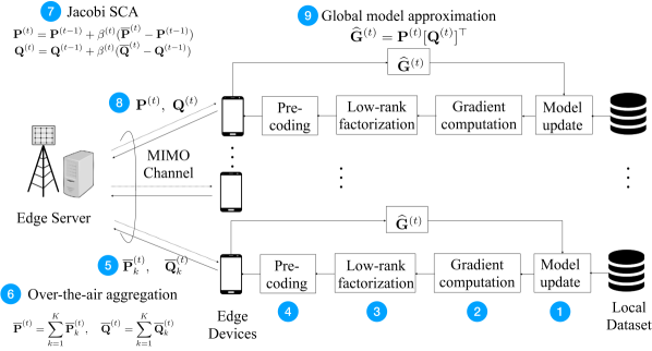
As shown in Fig. 1, we consider a federated edge learning (FEEL) system comprising a single edge server and edge devices connected via a shared MIMO channel. Each device has its local dataset . This consists of labeled data samples , where denotes the covariates and denotes the associated label, which may be continuous or discrete. A tensor is collaboratively trained by the edge devices through communications via the edge server.
II-1 Federated Gradient Descent
The local loss function for the -th device evaluated at parameter tensor is given by
| (1) |
where is the sample-wise loss function quantifying the prediction error of the model on the training sample with respect to (w.r.t.) its ground-truth label ; and is the cardinality of data set . Accordingly, the global loss function is given as
| (2) |
where . The federated learning process aims to minimize the global loss function as
| (3) |
At each -th communication round, by using the current model and the local dataset , each device computes the gradients of the local loss function in (1), that is
| (4) |
The devices transmit information about the local gradient in (4) over a shared wireless channel to the edge server. Based on the received signal, the edge server obtains the global gradient
| (5) |
where is the local gradient for device . The edge server updates the model via gradient descent
| (6) |
where denotes the learning rate. The updated parameter tensor (6) is sent back to all devices on the downlink. As in much of previous works such as [8, 7, 13], we assume that downlink communication is ideal, which is practically well justified when the edge server communicates with a less stringent power constraint than the devices. The steps in (4)-(6) are repeated until a convergence condition is met.
II-2 Communication Model
We now introduce the uplink wireless MIMO communication model for the FL system. Each device is equipped with transmitted antennas, and the server is equipped with received antennas. In the -th communication round, all devices communicate their local gradients through a block-fading channel simultaneously. We assume the channel state information (CSI) remains constant within communication blocks. The received signal over the blocks in a coherence period is given as
| (7) |
where is the MIMO channel between the -th device and the server, is the transmit signal of device , and is the channel noise with identical and independent distributed elements following distribution . As in [15], we assume that the CSI is known to the server, and not each device has access to the local CSI . The average transmit power constraints at each device across all antennas equals .
III Low-Rank Gradient Compression with Error Feedback
In this section, we present the proposed over-the-air low-rank compression (Ota-LC) method. Ota-LC reduces the communication overhead by imposing a low-rank parameterization to subtensors of tensor , which is known to serve as a useful inductive bias in many learning problems [11, 16]. We also exploit the temporal correlations exhibited by gradients across iterative steps [17], as well as analog communication [18] and error feedback, with the latter aiming at a reduction of the bias of the low-rank compressed gradient [19].
III-A Overview
To reduce the communication overhead, Ota-LC applies a low-rank matrix factorization separately to subtensors of the overall gradient tensor . The approach applies to a wide range of neural network architectures, including multilayer perceptrons, convolutional networks, graph neural networks, and transformers. In fact, the high-dimension tensor of these models’ parameters can be partitioned into sub-tensors that can be reshaped into matrices suitable for low-rank factorization. For example, the gradient of a CNN takes the form of a 4-D tensor , where represents the number of output channels, is the number of input channels, and denotes the kernel size. For CNNs, one way to obtain sub-tensors is by partitioning along the dimension of the output channels [11].
Low-rank compression is carried out in a distributed way by means of one step of a Jacobi SCA iteration [20] for a factorization problem. This step leverages temporal correlation across iterations by adopting an initialization based on the last iterate, and it also incorporates error feedback.
At each iteration, the devices transmit the updated local factorization matrices through the wireless MIMO channel using analog modulation. The server recovers the sum of the local factorizations from the received signal via over-the-air computation to obtain the low-rank factorizations of the global gradient. Ota-LC is summarized in Algorithm 1, and a detailed explanation is provided next.
III-B Low-Rank Gradient Compression
We start by describing low-rank compression (LC) for matrix factorization in the ideal case of a centralized system. We write, with some abuse of notation, as any one of the subtensors in which the gradient is partitioned. We reshape such subtensor into an matrix, also denoted as .
The high-dimensional gradient matrix is represented by using low-rank matrices and with rank , as . Finding the optimal matrix factorization is formulated as the minimization [21]
| (8) |
where is a regularization parameter, which controls the norms of factors and , and denotes the Frobenius norm of a matrix. The problem (8) is biconvex [22], and a centralized algorithmic solution is given by Jacobi SCA [20, Algorithm 1].
To elaborate, given initialization and , for each round , Jacobi SCA solves two surrogate convex problems
| (9) |
| (10) |
in parallel, where and represent the current iterates. Closed-form optimal solution for problems (9) and (10) are
| (11) | ||||
where is the identity matrix. Then, the updated factors are
| (12) | ||||
where is the step size of the update (12). At the last round , we obtain an approximation of global gradient as . As a remark, when , the update (12) is equivalent to the classical Jacobi best-response scheme, and its Gauss-Seidel counterpart update corresponds to alternating least squares (ALS) [23].
III-C Distributed LC
Consider now a distributed setting. In this case, by (5), the gradient matrix is obtained as the sum , where matrix is available at the -th device. Plugging into (11), we can write the update (11) as the sums
| (13) |
where the pair and is evaluated at device with in lieu of . This approach, however, requires a large communication overhead, as low-rank factors and must be exchanged across the rounds of the LC update in (12).
III-D Ota-LC: Protocol
To address this issue, at each round of federated gradient descent, Ota-LC produces updated low-rank factors and by using the previous iterates and as the starting point, for a single step of update (12), i.e., for . More precisely, we consider a parallel version of the calculation (11) given by
| (14) | ||||
for each round , yielding the updated low-rank factor and
| (15) | ||||
This approach is motivated by the observation that gradients typically exhibit strong temporal correlations across iterations [11, 17].
In Ota-LC, the local devices only need to upload two low-dimensional matrices and instead of the original high-dimensional local gradient . The communication overhead is thus reduced from to . In terms of computational complexity, the local updates (14) require an order of basic operation.
III-E Ota-LC: Signal Design
In Ota-LC, the aggregation (13) is implemented using over-the-air computation to enhance spectrum efficiency. To start, we stack the obtained and in (14) as the matrix to be further processed for transmission. At each device , the matrix is then arranged into a complex matrix as in, e.g., [7, 8].
The rank dictates the length of the communication blocks. In particular, with transmit antennas, the number of required channel uses in the time-frequency domain is
| (16) |
where all antennas transmit different entries of each .
Let denote the receive beamforming matrix and let denote the transmit beamforming matrix of device at iteration . We assume that the server can accurately estimate the CSI of each device to obtain the beamforming matrices. We use the over-the-air beamforming method in [24], and hence the beamforming matrices are designed as
| (17) | ||||
where is given as , where and are obtained by compact singular value decomposition (SVD) of as . Then, the transmit signal of each device at each iteration is
| (18) |
where is obtained by reshaping the matrix . We assume the inequality, , which can be satisfied by choosing suitably the rank .
At the server, by using the receive beamforming in (17), the recovered signal is an approximation of the sum given as
| (19) |
Then, the server first reshapes matrix into as an estimate of the sum , and it transforms matrix into real matrix , which is an estimate of the sum . The first columns of yield , and the remaining columns yield . The matrix and are used for update in (15) in lieu of and .
III-F Ota-LC: Error feedback
To alleviate the impact of the low-rank approximation error, Ota-LC introduces an error feedback mechanism in a manner similar to [25]. Accordingly, the local gradient is modified as
| (20) |
where is the approximation error, which initialized as . The local gradient factorization step (14) is applied to the error-compensated gradient . The compression error attached with device is set as
| (21) |
IV Numerical Experiments
We consider a wireless federated learning system with one server and edge devices. In each communication round, only a randomly selected half of the devices upload their local gradients to the server. The transmit SNR is set to dB. The number of transmitter antennas of each device is set as , and the number of the receive antennas of the server as . The entries of the communication channels are generated from i.i.d. for all and . The channels are assumed to be constant within each iteration .
The experiments were performed on the classification task for the Cifar-10 dataset. We flipped and cropped the dataset for data augmentation to avoid overfitting as in [26, 27]. We use the CNN model ResNet18, setting the learning rate as , and the weight in LC update to for all . We control the number of parameters uploaded by the local devices by changing the value of the rank . Our method is compared with SGD without compression, as well as with three existing gradient compression methods for wireless federated learning, as detailed next.
Ota-CS [7]: Ota-CS employs Turbo-CS, a compressed sensing technique detailed in [14], to compress the transmitted gradients. Specifically, the method sparsifies the vectorized gradients after projection into a subspace of dimension via multiplication by an partial discrete Fourier transform (DFT) compression matrix. This operation has a complexity of order . This amounts to an increase of order as compared to the complexity of for Ota-LC. The server then reconstructs the compressed gradients using Turbo-CS. This method leverages over-the-air computation for data transmission.
BLUE-CS [8]: Similar to Ota-CS, BLUE-CS utilizes Turbo-CS for gradient compression, but, during data transmission, it adopts the best linear unbiased estimator (BLUE) algorithm to independently recover transmitted signals at the server, rather than leveraging over-the-air computing.
Ota-RLC[13]: In Ota-RLC, gradient compression employs RLC as introduced in [10]. The local device first multiplies the vectorized gradients with a partial Hadamard matrix , featuring mutually orthogonal rows, entailing a local computation cost of order as for Ota-CS. The server recovers the compressed gradient, using over-the-air computation for gradient transmission.
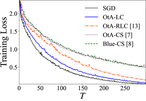
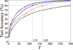
We first provide a convergence performance comparison by evaluating training loss and test accuracy against the number of communication rounds for channel uses and . It can be observed in Fig. 2 that the proposed Ota-LC approach has a similar test accuracy at the last round as SGD while demonstrating a faster convergence rate than other methods. For instance, when aiming a learning accuracy of in Fig. 3, iterations are needed for BLUE-CS and Ota-CS, iterations for Ota-RLC, while Ota-LC requires only iterations. Thus, to attain equivalent performance, Ota-CS reduces the communication overhead by .
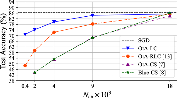
Then, we compare Ota-LC with the mentioned benchmarks for different numbers of channel uses over communication rounds. The results in Fig. 3 show that Ota-LC performs better under the same communication overhead, especially in the regime of a low number of communication resources , which corresponds to the case of a more aggressive compression ratio.
V Conclusion
In this letter, we have proposed Ota-LC, a gradient compression and transmission method that reduces the communication overhead for MIMO wireless federated learning. Experimental results show Ota-LC converges faster and has better performance than existing benchmarks [8, 7, 13], while having smaller communication and computational costs. Future work may investigate the fully decentralized extension of Ota-LC.
References
- [1] J. Dean, G. Corrado, R. Monga, K. Chen, M. Devin, M. Mao, M. Ranzato, A. Senior, P. Tucker, K. Yang et al., “Large scale distributed deep networks,” in Proc. Adv. Neural Info. Proc. Syst. (NIPS), (Lake Tahoe, USA), Dec. 2012.
- [2] D. Alistarh, D. Grubic, J. Li, R. Tomioka, and M. Vojnovic, “QSGD: Communication-efficient sgd via gradient quantization and encoding,” in Proc. Adv. Neural Info. Proc. Syst. (NIPS), (Long Beach, USA), Dec. 2017.
- [3] J. Bernstein, Y.-X. Wang, K. Azizzadenesheli, and A. Anandkumar, “SignSGD: Compressed optimisation for non-convex problems,” in Proc. Int. Conf. Mach. Learn., (Stockholm, Sweden), Jul. 2018.
- [4] D. Alistarh, T. Hoefler, M. Johansson, N. Konstantinov, S. Khirirat, and C. Renggli, “The convergence of sparsified gradient methods,” in Proc. Adv. Neural Info. Proc. Syst. (NIPS), (Montréal, Canada), Dec. 2018.
- [5] S. U. Stich, J.-B. Cordonnier, and M. Jaggi, “Sparsified SGD with memory,” in Proc. Adv. Neural Info. Proc. Syst. (NIPS), (Montréal, Canada), Dec. 2018.
- [6] A. Sahu, A. Dutta, A. M Abdelmoniem, T. Banerjee, M. Canini, and P. Kalnis, “Rethinking gradient sparsification as total error minimization,” in Proc. Adv. Neural Info. Proc. Syst. (NIPS), (Virtual), Dec. 2021.
- [7] C. Zhong and X. Yuan, “Over-the-air federated learning over MIMO channels: A sparse-coded multiplexing approach,” [Online]. Available: https://arxiv.org/pdf/2304.04402.pdf, 2023.
- [8] E. Becirovic, Z. Chen, and E. G. Larsson, “Optimal MIMO combining for blind federated edge learning with gradient sparsification,” in Proc. 2022 IEEE 23rd Int. Workshop Signal Process. Adv. Wireless Commun. (SPAWC), (Oilu, Finland), Jul. 2022.
- [9] Y.-S. Jeon, M. M. Amiri, J. Li, and H. V. Poor, “A compressive sensing approach for federated learning over massive MIMO communication systems,” IEEE Trans. Wireless Commun., vol. 20, no. 3, pp. 1990–2004, 2020.
- [10] A. Abdi, Y. M. Saidutta, and F. Fekri, “Analog compression and communication for federated learning over wireless mac,” in Proc. 2020 IEEE 21st Int. Workshop Signal Process. Adv. Wireless Commun. (SPAWC), (Virtual), May. 2020.
- [11] T. Vogels, S. P. Karimireddy, and M. Jaggi, “PowerSGD: Practical low-rank gradient compression for distributed optimization,” in Proc. Adv. Neural Info. Proc. Syst. (NIPS), (Vancouver, Canada), Dec. 2019.
- [12] A. V. Makkuva, M. Bondaschi, T. Vogels, M. Jaggi, H. Kim, and M. C. Gastpar, “Laser: Linear compression in wireless distributed optimization,” [Online]. Available: https://arxiv.org/pdf/2310.13033.pdf, 2023.
- [13] H. Xing, O. Simeone, and S. Bi, “Federated learning over wireless device-to-device networks: Algorithms and convergence analysis,” IEEE J. Sel. Areas Commun., vol. 39, no. 12, pp. 3723–3741, 2021.
- [14] J. Ma, X. Yuan, and L. Ping, “Turbo compressed sensing with partial dft sensing matrix,” IEEE Signal Process. Lett., vol. 22, no. 2, pp. 158–161, 2015.
- [15] K. Yang, T. Jiang, Y. Shi, and Z. Ding, “Federated learning via over-the-air computation,” IEEE Trans. Wireless Commun., vol. 19, no. 3, pp. 2022–2035, 2020.
- [16] G. K. Dziugaite and D. M. Roy, “Neural network matrix factorization,” [Online]. Available: https://arxiv.org/pdf/1511.06443.pdf, 2015.
- [17] S. S. Azam, S. Hosseinalipour, Q. Qiu, and C. Brinton, “Recycling model updates in federated learning: Are gradient subspaces low-rank?” in Proc. Int. Conf. Learn. Represent., (Virtual), May. 2021.
- [18] T. L. Marzetta, E. G. Larsson, H. Yang, and H. Q. Ngo, Fundamentals of Massive MIMO. Cambridge University Press, 2016.
- [19] A. F. Aji and K. Heafield, “Sparse communication for distributed gradient descent,” [Online]. Available: https://arxiv.org/pdf/1704.05021.pdf, 2017.
- [20] G. Scutari, F. Facchinei, P. Song, D. P. Palomar, and J.-S. Pang, “Decomposition by partial linearization: Parallel optimization of multi-agent systems,” IEEE Trans. Signal Process., vol. 62, no. 3, pp. 641–656, 2014.
- [21] Y. Koren, R. Bell, and C. Volinsky, “Matrix factorization techniques for recommender systems,” Computer, vol. 42, no. 8, pp. 30–37, 2009.
- [22] T. Hastie, R. Mazumder, J. D. Lee, and R. Zadeh, “Matrix completion and low-rank svd via fast alternating least squares,” J. Mach. Learn. Res., vol. 16, no. 1, pp. 3367–3402, 2015.
- [23] P. Jain, P. Netrapalli, and S. Sanghavi, “Low-rank matrix completion using alternating minimization,” in Proc. of the forty-fifth annual ACM symposium on Theory of computing, (Palo Alto, USA), Jun. 2013.
- [24] G. Zhu and K. Huang, “MIMO over-the-air computation for high-mobility multimodal sensing,” IEEE Internet Things J., vol. 6, no. 4, pp. 6089–6103, 2018.
- [25] S. P. Karimireddy, Q. Rebjock, S. Stich, and M. Jaggi, “Error feedback fixes signsgd and other gradient compression schemes,” in Proc. Int. Conf. Mach. Learn., (Long Beach, USA), Jun. 2019.
- [26] Y. Lecun, L. Bottou, Y. Bengio, and P. Haffner, “Gradient-based learning applied to document recognition,” Proc. of the IEEE, vol. 86, no. 11, pp. 2278–2324, 1998.
- [27] A. Krizhevsky, I. Sutskever, and G. E. Hinton, “ImageNet classification with deep convolutional neural networks,” in Proc. Adv. Neural Info. Proc. Syst. (NIPS), (Lake Tahoe, USA), Dec. 2012.