Input Convex Lipschitz RNN: A Fast and Robust Approach for Engineering Tasks

Abstract

Computational efficiency and adversarial robustness are critical factors in real-world engineering applications. Yet, conventional neural networks often fall short in addressing both simultaneously, or even separately. Drawing insights from natural physical systems and existing literature, it is known that an input convex architecture enhances computational efficiency, while a Lipschitz-constrained architecture bolsters adversarial robustness. By leveraging the strengths of convexity and Lipschitz continuity, we develop a novel network architecture, termed Input Convex Lipschitz Recurrent Neural Networks. This model outperforms existing recurrent units across a spectrum of engineering tasks in terms of computational efficiency and adversarial robustness. These tasks encompass a benchmark MNIST image classification, real-world solar irradiance prediction for Solar PV system planning at LHT Holdings in Singapore, and real-time Model Predictive Control optimization for a chemical reactor.

I Introduction

Two crucial criteria for the resolution of real-world engineering challenges are computational efficiency and adversarial robustness. This big-data era has empowered the capabilities of neural networks and transformed them into an incredibly powerful tool, offering comprehensive solutions to numerous engineering problems such as image classification and process modeling. This work draws inspiration from nature-inspired design to develop a fast and robust solution to model nonlinear systems in various engineering disciplines.

Model Predictive Control (MPC) represents an advanced control technique applied to manage a process while complying with a set of constraints, akin to an optimization challenge. Traditional MPC based on first-principles models encounters limitations, particularly in scenarios with intricate dynamics, where deriving these models proves infeasible. Consequently, researchers proposed neural network-based MPC (NN-MPC) as a viable alternative to model system dynamics [1, 2, 3, 4, 5, 6, 7, 8]. However, MPC built on conventional neural networks often falls short in meeting the aforementioned critical criteria. Nonetheless, efforts have been made to mitigate these limitations. For example, the computational efficiency of NN-MPC is enhanced by implementing an input convex architecture in neural networks [9]. Additionally, adversarial robustness of NN-MPC is improved by developing Lipschitz-constrained neural networks (LNNs) [10].

In real-world applications, computational efficiency plays a pivotal role due to the imperative need for real-time decision-making, especially in critical engineering processes such as chemical process operations [9]. We define computational efficiency as the speed at which computational tasks are completed within a given execution timeframe. An effective approach to achieve this efficiency is through the transformation from non-convex to convex structures. Convexity is an ubiquitous characteristic observed in various physical systems. In energy potentials, the potential energy function of certain systems, such as simple harmonic oscillators, can exhibit a convex behavior. For example, the potential energy function of a mass on a spring is a classic example of a convex function in physics [11, 12]. In the context of magnetic fields, the region around a single magnetic pole, where another magnetic pole encounters an attractive force, is considered convex [13, 14]. In the theory of general relativity, the curvature of space-time around massive objects like stars or black holes can be described as convex in certain regions. This curvature influences the paths of objects and light rays near these massive bodies [15].

Building upon nature-inspired design and extending its application to neural networks, Input Convex Neural Networks (ICNNs) is a class of neural network architectures intentionally crafted to maintain convexity in their output with respect to the input. Leveraging these models could be particularly advantageous in various engineering problems, notably in applications such as MPC, due to their inherent benefits especially in optimization. This concept was first introduced by [16] as Feedforward Neural Networks (FNN), and subsequently extended to Recurrent Neural Networks (RNN) by [17], and Long Short-Term Memory (LSTM) by [9].

Additionally, in real-world engineering applications, adversarial robustness plays a critical role due to the prevalent noise present in most real-world data, which significantly hampers neural network performance. Our definition of robustness aligns closely with the principles outlined by [10]. Given the inherent noise in real-world process data, our goal is to improve neural networks by effectively learning from noisy training data for comprehensive end-to-end applications. Leveraging LNNs offers a potential solution to the robustness challenge. This concept was first introduced by [18] as FNN, and subsequently extended to RNN by [19], and Convolutional Neural Networks (CNN) by [20].

Motivated by the above considerations, in this work, we introduce an Input Convex Lipschitz RNN (ICLRNN) that amalgamates the strengths of ICNNs and LNNs. This approach aims to achieve the concurrent resolution of computational efficiency and adversarial robustness, which remains a challenge in real-world engineering applications. While the primary motivation of this work centers on crafting a fast and robust MPC framework, we endeavor to showcase the versatile applicability of ICLRNN beyond MPC. Therefore, in this study, we validate the efficacy of ICLRNN across various engineering problems that include image classification, time series forecasting, and neural network-based MPC. Specifically, we employ a publicly available dataset MNIST [21] for image classification. For time-series forecasting, we engage in planning for Solar Photovoltaic (PV) systems with real-time data from LHT Holdings plants in Singapore. Furthermore, we use a nonlinear chemical reactor example to show the benefits of ICLRNN in the context of MPC.

In summary, Section II offers an overview of modern ICNNs and LNNs. Section III presents the proposed ICLRNN, substantiating its theoretical attributes as input convex and Lipschitz continuous. In Section IV, we illustrate that ICLRNN surpasses state-of-the-art RNN units in various engineering tasks, including image classification, real-time solar irradiance forecasting on Solar PV systems, and optimization and control of chemical processes using MPC.

II Background

II-A Notations

Let $L(f)$ represents the Lipschitz constant of a function $f$. $``\circ"$ denotes composition. $\|\cdot\|$, $\|\cdot\|_{2}$, and $\|\cdot\|_{F}$ denote spectral norm, Euclidean norm, and Frobenius norm of a matrix respectively. $\sigma(\cdot)$ denotes the singular value of a matrix and $r(\cdot)$ denotes the rank of a matrix. For neural networks, $x$ denotes the input, $g$ denotes the activation function, $W$ denotes the weights, $h$ denotes the hidden state, and $y$ denotes the output.

II-B Input Convex RNN

Definition 1.

A function $f:X\rightarrow\mathbb{R}$ is convex if and only if the following inequality holds $\forall\leavevmode\nobreak\ (x_{1},x_{2})\in X$, with $x_{1}\neq x_{2}$, and $\forall\leavevmode\nobreak\ \lambda\in(0,1)$:

$$f(\lambda x_{1}+(1-\lambda)x_{2})\leq\lambda f(x_{1})+(1-\lambda)f(x_{2})$$

and it is strictly convex if the relation $\leq$ becomes $<$.

The initiative behind ICNNs is to leverage the power of neural networks, specifically designed to maintain convexity within their decision boundaries [16]. ICNNs aim to combine the strengths of neural networks in modeling complex data with the advantages of convex optimization, which ensures the convergence to a global optimal solution. They are particularly attractive for control and optimization problems, where achieving globally optimal solutions is essential. By maintaining convexity, ICNNs help ensure that the optimization problems associated with neural networks (e.g., neural network-based optimization) remain tractable, thus addressing some of the challenges of non-convexity and the potential for suboptimal local solutions in traditional neural networks.

A foundational work, known as Input Convex RNN (ICRNN), serves as one of the baselines in this paper. The output of ICRNN follows [17]:

$$\begin{split}h_{t}&=g_{1}(U\textbf{x}_{t}+Wh_{t-1}+D_{2}\textbf{x}_{t-1})\\ y_{t}&=g_{2}(Vh_{t}+D_{1}h_{t-1}+D_{3}\textbf{x}_{t})\end{split}$$

The output $y_{t}$ is convex with respect to the input x if non-decreasing and convex activation functions are used for $g$, and $[D3,D2,D1,V,W,U]$ are chosen to be non-negative weights, where x denotes $\big{[}\begin{smallmatrix}x\\ -x\end{smallmatrix}\big{]}$.

II-C Lipschitz RNN

Definition 2.

A function $f:X\rightarrow\mathbb{R}$ is Lipschitz continuous with Lipschitz constant $L$ (i.e., L-Lipschitz) if and only if the following inequality holds $\forall\leavevmode\nobreak\ (x_{1},x_{2})\in X$:

$$\|f(x_{1})-f(x_{2})\|_{2}\leq L\|x_{1}-x_{2}\|_{2}$$

By adhering to the definition of Lipschitz continuity for a function $f$, where an L-Lipschitz continuous $f$ ensures that any minor perturbation to the input results in an output change of at most $L$ times the magnitude of that perturbation. Therefore, constraining neural networks to maintain Lipschitz continuity significantly fortifies their resilience against input perturbations.

A pivotal work, namely the Lipschitz RNN (LRNN), stands as one of the baselines in this paper. The output of LRNN follows [19]:

$$\begin{split}\dot{h}&=A_{\beta_{A},\gamma_{A}}h+tanh(W_{\beta_{W},\gamma_{W}}h+Ux+b)\\ y&=Dh\end{split}$$

where $\beta_{A},\beta_{W}\in[0,1]$, $\gamma_{A},\gamma_{W}>0$ are tunable parameters, $M_{A},M_{W},D,U$ are trainable weights, $\dot{h}$ is the time derivative of $h$ (i.e., $h$ can be updated by the explicit (forward) Euler scheme or a two-stage explicit Runge-Kutta scheme), and $A_{\beta_{A},\gamma_{A}},W_{\beta_{W},\gamma_{W}}$ is computed as follows:

$$\begin{split}A_{\beta_{A},\gamma_{A}}=&(1-\beta_{A})(M_{A}+M_{A}^{T})+\beta_{A}(M_{A}-M_{A}^{T})\\ &-\gamma_{A}I\\ W_{\beta_{W},\gamma_{W}}=&(1-\beta_{W})(M_{W}+M_{W}^{T})+\beta_{W}(M_{W}-M_{W}^{T})\\ &-\gamma_{W}I\end{split}$$

III Input Convex Lipschitz Recurrent Neural Networks

In this section, we develop a novel network architecture, termed ICLRNN, that possesses both Lipschitz continuity and input convexity properties. Specifically, the output of ICLRNN is defined as follows:

$$h_{t}=g_{1}(W_{t}^{x}x_{t}+W_{t}^{h}h_{t-1}+b_{t}^{h})$$ (1a)

$$y_{t}=g_{2}(W_{t}^{y}h_{t}+b_{t}^{y})$$ (1b)

where all $W_{i}$ are constrained to be non-negative with singular values small and bounded by $\mathcal{O}(1)$, and all $g_{i}$ are constrained to be convex, non-decreasing, and Lipschitz continuous.

The output of a neural network inherits input convexity and Lipschitz continuity if and only if every hidden state possesses these properties. Unlike [17] and [19], our ICLRNN adheres to this foundational principle by imposing constraints on the weights and activation functions instead of introducing supplementary variables to the original RNN architecture. This approach minimizes the demand of computational resources. We first introduce a proposition to demonstrate that imposing an input convex constraint subsequent to a Lipschitz constraint does not compromise the latter.

Proposition 1.

Let $A$ be an $m\times n$ matrix with its largest singular value at most 1. If all negative elements in matrix $A$ are replaced by 0 to obtain a non-negative matrix $B$, then the largest singular value of matrix $B$ remains small and bounded by $\sqrt{r(A)}$, and further bounded by $\sqrt{min(m,n)}$.

Proof.

We begin the proof with a commonly admitted fact:

$$\|A\|=\sigma_{max}(A)\leq\|A\|_{F}=(\sum_{ij}|a_{ij}|^{2})^{\frac{1}{2}}=(\sum_{k}\sigma_{k}^{2})^{\frac{1}{2}}$$ (2)

where $A$ is an $m\times n$ matrix with its largest singular value at most 1 (i.e., $\|A\|=\sigma_{max}(A)\leq 1$), $a_{ij}$ represents the elements in $A$, and the number of singular value $k$ is at most $min(m,n)$. Equality holds if and only if $A$ is a rank-one matrix or a zero matrix. Given that the rank of a matrix is precisely the number of non-zero singular values, we extend the inequality in Eq. (2) further:

$$\|A\|_{F}\leq(r(A)\sigma_{max}(A)^{2})^{\frac{1}{2}}=\sqrt{r(A)}\|A\|$$ (3)

where the equality holds if and only if all non-zero singular values are equal.

Let $B$ be a non-negative $m\times n$ matrix transformed by replacing all negative elements in $A$ with 0, where $b_{ij}$ represents the elements in $B$. Based on the transformation, we have the property:

$$|b_{ij}|^{2}\leq|a_{ij}|^{2}$$

Thus, the following inequality holds:

$$\|B\|\leq\|B\|_{F}=(\sum_{ij}|b_{ij}|^{2})^{\frac{1}{2}}\leq(\sum_{ij}|a_{ij}|^{2})^{\frac{1}{2}}=\|A\|_{F}$$ (4)

Based on Eq. (3) and (4) and the assumption that $\|A\|\leq 1$, we conclude:

$$\|B\|\leq\|A\|_{F}\leq\sqrt{r(A)}\|A\|\leq\sqrt{r(A)}\leq\sqrt{min(m,n)}$$

∎

For ICLRNN, we first enforce the spectral constraints to ensure that the largest singular values of the weight matrix is at most one [18]. The spectral constraint is implemented in two steps, which is similar to [20]. Firstly, we use spectral normalization as proposed by [22], where the spectral norm is reduced to at most 1 by iteratively evaluating the largest singular value with the power iteration algorithm proposed by [23]. Secondly, we apply the Björck algorithm proposed by [24] to increase other singular values to at most one.

Next, we enforce the non-negative constraint by performing weight clipping to set all negative values in the weights to 0. It is essential to note that the upper bound in Eq. (2) is not precisely tight [25], and thus the upper bound developed in Proposition 1 is not tight. Through experimentation on random large matrices and the experiments in Section IV, we have observed that the Lipschitz constant is normally bounded within the order of $\mathcal{O}(1)$.

Moreover, ICLRNN uses ReLU as the activation function for hidden states instead of the GroupSort function proposed in [18]. This decision aims to maintain convexity within the model architecture. Although GroupSort exhibits gradient norm preservation and higher expressive power [10], its non-convex nature contrasts with our primary objectives. Next, we will proceed to prove the convexity and Lipschitz continuity of ICLRNN.

III-A Convexity and Lipschitz Continuity of ICLRNN

The following lemmas are provided to prove Proposition 2 regarding the Lipschitz continuity of ICLRNN.

Lemma 1 ([26]).

Consider a set of functions, e.g., $f:X\rightarrow\mathbb{R}$ and $g:X\rightarrow\mathbb{R}$ with Lipschitz constants $L(f)$ and $L(g)$, respectively, by taking their sum, i.e., $h=f+g$, the Lipschitz constant $L(h)$ of $h$ satisfies:

$$L(h)\leq L(f)+L(g)$$

Lemma 2 ([26]).

Consider a set of functions, e.g., $f:X\rightarrow\mathbb{R}$ and $g:X\rightarrow\mathbb{R}$ with Lipschitz constants $L(f)$ and $L(g)$ respectively, by taking their composition, denoted as $h=f\circ g$, the Lipschitz constant $L(h)$ of the resultant function $h$ satisfies:

$$L(h)\leq L(f)\times L(g)$$

Lemma 3.

Given a linear function with a weight $W\in\mathbb{R}^{n\times m}$, we have:

$$L(W)=\|W\|=\sigma_{max}(W)$$

Lemma 4 ([27, 28]).

The most common activation functions such as ReLU, Sigmoid, and Tanh have a Lipschitz constant that equals 1, while Softmax has a Lipschitz constant bounded by 1.

Proposition 2.

The Lipschitz constant of an ICLRNN is $\mathcal{O}(1)$ if and only if all weights $W_{i}$ and all activation functions $g_{i}$ have a Lipschitz constant bounded by $\mathcal{O}(1)$.

Proof.

By unrolling the recurrent operations over time $t$ in Eq. (1), the output of ICLRNN can be described as a function:

$$\begin{split}f(x)=&g_{t}(W_{t}^{y}g_{t-1}^{h}(W_{t-1}^{x}x_{t-1}\\ &+W_{t-1}^{h}...g_{1}(W_{1}^{x}x_{1}+W_{1}^{h}h_{0})))\end{split}$$ (5)

The Lipschitz constant of an ICLRNN is upper bounded by the product of sum of the individual Lipschitz constants (i.e., Lemma 1 and Lemma 2):

$$\begin{split}L(f)\leq&L(g_{t})\times L(W_{t}^{y})\times L(g_{t-1})\times(L(W_{t-1}^{x})\\ &+L(W_{t-1}^{h})\times...L(g_{1})\times(L(W_{1}^{x})+L(W_{1}^{h})))\\ \end{split}$$

If we ensure that the Lipschitz constants of all $W_{i}$ in ICLRNN are $\mathcal{O}(1)$, the ICLRNN for classification tasks with ReLU activation for hidden states and Sigmoid or Softmax activation for output layer has a Lipschitz constant of $\mathcal{O}(1)$, while the ICLRNN for regression tasks with ReLU activation for hidden states and Linear activation for output layer has a Lipschitz constant of $\mathcal{O}(1)$ (i.e., Lemma 3 and Lemma 4). ∎

The following lemmas are provided to prove Proposition 3 regarding the convexity of ICLRNN.

Lemma 5 ([29]).

Consider a set of convex functions, e.g., $f:X\rightarrow\mathbb{R}$ and $g:X\rightarrow\mathbb{R}$, their weighted sum, i.e., $\alpha f+\beta g$, remains convex if coefficients $\alpha$ and $\beta$ are non-negative.

Lemma 6 ([29]).

Consider a convex function $f:X\rightarrow\mathbb{R}$ and a convex monotone non-decreasing function $g:X\rightarrow\mathbb{R}$, the composition of $f$ and $g$, denoted as $g\circ f$, is both convex and non-decreasing.

Proposition 3.

The output $y$ of an ICLRNN is input convex if and only if all $W_{i}$ are constrained to be non-negative and all $g_{i}$ are constrained to be convex and non-decreasing.

Proof.

By unrolling the recurrent operations over time $t$ in Eq. (1), the output of ICLRNN can be described as a function of Eq. (5). The output of an ICLRNN $y=f(x)$ is convex with respect to $x$ (i.e., Lemma 5 and Lemma 6). ∎

By combining Proposition 2 and Proposition 3, the following theorem can be readily derived without requiring additional proof.

Theorem 1.

The output $y$ of an L-layer Input Convex Lipschitz Recurrent Neural Network is a convex, non-decreasing, and Lipschitz continuous function with respect to the input $x$, where $x$ is in a convex feasible space $\mathcal{X}$, if and only if the following constraints on weights $W_{i}$ and activation functions $g_{i}$ are satisfied simultaneously: (1) All $W_{i}$ are constrained to be non-negative with singular values bounded by $\mathcal{O}(1)$; (2) All $g_{i}$ are constrained to be convex, non-decreasing, and Lipschitz continuous (e.g., ReLU, Linear, Softmax, Sigmoid).

Next, we proceed by developing a Lyapunov-based MPC (LMPC) framework. Our focus lies in showcasing the transformation of a non-convex NN-based LMPC into a convex optimization problem by utilizing ICNNs.

III-B ICLRNN for a Finite-Horizon Convex MPC

III-B1 Class of systems

Specifically, we examine a category of systems that can be expressed through a particular set of ordinary differential equations (ODE), given by the following form:

$$\dot{x}=F(x,u)$$ (6)

where $u\in\mathbb{R}^{m}$ denotes the control action and $x\in\mathbb{R}^{n}$ denotes the state vector. The function $F:X\times U\to\mathbb{R}^{n}$ is continuously differentiable, where $X\subset\mathbb{R}^{n}$ and $U\subset\mathbb{R}^{m}$ are connected and compact subsets that enclose an open neighborhood around the origin respectively. In this context, we maintain the assumption throughout this task that $F(0,0)=0$, ensuring that the origin $(x,u)=(0,0)$ serves as an equilibrium point. As it might be impractical to obtain first-principles models for intricate real-world systems, our objective is to construct a neural network to model the nonlinear system specified by Eq. (6), embed it into MPC, and maintain computational efficiency and adversarial robustness of MPC simultaneously.

III-B2 LMPC formulation

The optimization problem of the LMPC scheme, which incorporates a neural network model as its predictive element, is expressed as follows [30]:

$$\mathcal{L}=\min_{u\in S(\triangle)}\int_{t_{k}}^{t_{k+N}}J(\tilde{x}(t),u(t))dt$$ (7a)

$$s.t.\ \dot{\tilde{x}}(t)=F_{nn}(\tilde{x}(t),u(t))$$ (7b)

$$u(t)\in U,\ \forall t\in[t_{k},t_{k+N})$$ (7c)

$$\tilde{x}(t_{k})=x(t_{k})$$ (7d)

$$V({\tilde{x}}(t))<V({x}(t_{k})),\forall t\in[t_{k},t_{k+N})$$ (7e)

where $S(\triangle)$ denotes the set of piecewise constant functions with period $\triangle$, $\tilde{x}$ denotes the predicted state trajectory, and $N$ denotes the number of sampling periods in the prediction horizon. The objective function $\mathcal{L}$ outlined in Eq. (7a) integrates a cost function $J$ that depends on both the control actions $u$ and the system states $x$. The system dynamic function $F_{nn}(\tilde{x}(t),u(t))$ expressed in Eq. (7b) is parameterized by an RNN (e.g., the proposed ICLRNN in this work). Eq. (7c) encapsulates the constraint function $U$, delineating feasible control actions. Eq. (7d) establishes the initial condition $\tilde{x}(t_{k})$ in Eq. (7b), referring to the state measurement at $t=t_{k}$. Lastly, Eq. (7e) represents the Lyapunov-based constraint $V$, ensuring closed-loop stability within LMPC by mandating a decrease in the value of $V(x)$ over time.

Remark 1 ([9]).

A convex neural network-based LMPC remains convex even when making multi-step ahead predictions, where the prediction horizon is greater than 1. This statement holds true if we incorporate an inherently input convex neural network (e.g., ICLRNN) to the LMPC, as described in Eq. (7b), and if we guarantee that the cost function $J$ in Eq. (7a) is input convex throughout the task.

IV Empirical Evaluation

In this section, we assess the performance of the proposed ICLRNN by benchmarking it against other state-of-the-art recurrent units. We aim to exhibit the computational efficiency and adversarial robustness of ICLRNN across various engineering challenges, spanning MNIST classification, solar irradiance prediction for Solar PV system utilizing real-time data from LHT Holdings plants (NUS-SIMTech project), and lastly, in implementing an NN-MPC for a chemical reactor. It should be pointed out that ablation studies are conducted to determine the optimal hyperparameter values for all the following tasks.

IV-A MINST Classification

Sequentially, we feed 784 pixels into the recurrent unit, akin to the approach outlined by [31], for classification purposes. All models are trained and evaluated under identical settings – utilizing Categorical Cross-entropy Loss, the Adam Optimizer [32], the ReLU activation function for hidden states [33], except for LRNN (i.e., Tanh activation function is used for LRNN as specified by [19]), maintaining a learning rate of 0.001, and employing a batch size of 128. The comprehensive analysis of results are discussed in Appendix A.

IV-A1 Computational Efficiency Analysis

To assess the computational efficiency among various models, we measure their respective Floating Point Operations per Second (FLOPs). Table I highlights that ICLRNN exhibits the lowest FLOPs, consequently surpassing or matching state-of-the-art methods. While LRNN exhibits a relatively small number of trainable parameters, its FLOPs are notably high, indicating its computational intensity. Additionally, ICRNN encounters challenges related to vanishing or exploding gradient problems when the network complexity exceeds certain thresholds.

Table I: Model complexity with layer size of (64, 64) for MNIST.

Model	Trainable Parameters	FLOPs
RNN	14,858	29,756
LSTM	57,482	115,516
ICRNN	42,890	86,332
LRNN	23,050	161,340
ICLRNN (ours)	14,858	29,756

IV-A2 Adversarial Robustness Analysis

To examine the adversarial robustness of ICLRNN, we analyze the sensitivity of the model’s response with respect to test accuracy when subjected to a sequence of perturbed inputs affected by Salt and Pepper noise. As depicted in Fig. 1, and Fig. 4 in Appendix A, the results demonstrate that ICLRNN consistently outperforms or matches state-of-the-art models across various levels of noise.

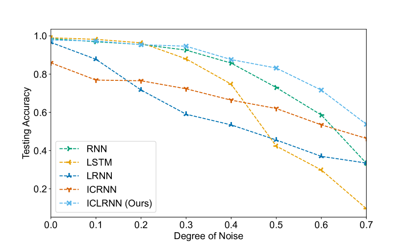
Figure 1: Model performance with layer size of (64, 64) w.r.t different degrees of Salt and Pepper noise for MNIST.

IV-B Real-World Solar Irradiance Prediction

In this task, we aim to forecast solar irradiance using real-time data sourced from LHT Holdings, a notable wood pallet manufacturing industry based in Singapore (for a detailed manufacturing pipeline of LHT Holdings, refer to Fig. 5 in Appendix B). Before the installation of the Solar photovoltaic (PV) system, LHT Holdings relied solely on the main utility grid to fulfill its energy needs. The Solar PV system was successfully installed by 10 Degree Solar in late 2022, as depicted in Fig. 7 in Appendix B. This transition to solar energy was primarily driven by the aim to minimize manufacturing costs. Three significant uncertainties were identified within the industry, namely solar irradiance affecting the Solar PV system’s efficiency, the dynamic real-time pricing of energy sourced from the main utility grid, and the fluctuating energy demand stemming from unexpected customer orders.

At present, the Solar PV system serves as the primary energy source for the industrial facility, while the main utility grid acts as a secondary energy source to supplement any deficiencies in solar energy production. Any surplus solar energy generated beyond the current requirements is efficiently stored in batteries for future utilization (i.e., see Fig. 6 in Appendix B). Hence, in order to optimize real-time energy planning and mitigate manufacturing costs associated with energy procurement from the main utility grid, a high level of precision and accuracy in forecasting solar irradiance becomes imperative. To achieve this goal, the Solar Energy Research Institute of Singapore (SERIS) has played a pivotal role by installing various sensors specifically designed for the Solar PV system. These sensors include irradiance sensors, humidity sensors, wind sensors, and module temperature sensors. Drawing on parameters akin to those employed by [34], we utilize minute-based average global solar irradiance, ambient humidity, module temperature, wind speed, and wind direction to predict solar irradiance in the subsequent minute.

In this time-series forecasting task, all models undergo training and evaluation using identical settings. These settings encompass the mean squared error as the loss function, the Adam Optimizer, the ReLU activation function except for LRNN, a consistent batch size of 256, and a fixed learning rate set at 0.001. For the training and validation phases, we use data spanning from January 14, 2023, to December 16, 2023. Subsequently, data from December 17, 2023, to January 1, 2024, is exclusively reserved for testing and evaluating the models’ predictive performance. The comprehensive discussion of results is accessible in Appendix B.

IV-B1 Computational Efficiency Analysis

Building upon our previous task on MNIST, we once again leverage FLOPs as a measure to assess the computational efficiency of models. As depicted in Table II, it is evident that among the models compared, ICLRNN demonstrates the most efficient computational performance as a result of its lowest FLOPs. Consequently, this superior efficiency positions ICLRNN as the top-performing model within this context when considering computational resources.

Table II: Model complexity with layer size of (256, 256) for solar irradiance prediction.

Model	Trainable Parameters	FLOPs
RNN	199,682	399,362
LSTM	797,186	1,596,418
ICRNN	596,482	1,195,010
LRNN	330,754	2,498,562
ICLRNN (ours)	199,682	399,362

IV-B2 Adversarial Robustness Analysis

Given the real-world context of this task, introducing artificial noise for evaluating adversarial robustness becomes unnecessary as the inherent noise within real-world data suffices. Notably, our observations reveal that ICRNN encounters challenges with the exploding gradient problem when the hypothesis space size is large (i.e., the number of hidden neurons per layer is more than 128), thereby hindering its ability to effectively model complex system dynamics. While RNN and LSTM exhibit a limited capacity to capture system dynamics, they struggle notably when faced with sudden changes in solar irradiance, leading to less accurate predictions.

In Fig. 2, we present results from the best state-of-the-art model, LRNN, alongside our model’s outcomes specifically for December 28, 2023. LRNN displays marked improvements compared to RNN and LSTM, yet it falls short in accurately predicting solar irradiance during sudden fluctuations. Additionally, during periods of minimal solar irradiance at the start and end of the day, LRNN exhibits slight fluctuations. Highlighted within Fig. 2, our ICLRNN outperforms LRNN, particularly in accurately predicting sudden changes in solar irradiance. This highlights the superior predictive capability of ICLRNN, showcasing its effectiveness in capturing and predicting nuanced fluctuations within the solar irradiance data. Notably, these observations persist across all trials and are not specific solely to December 28, 2023.

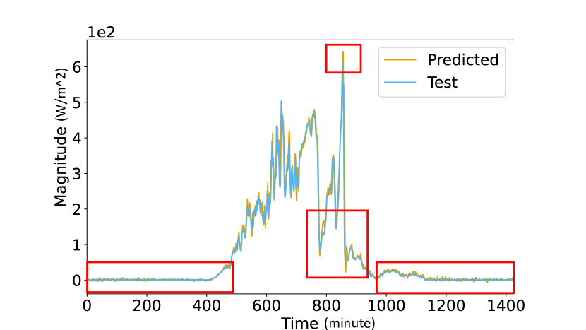
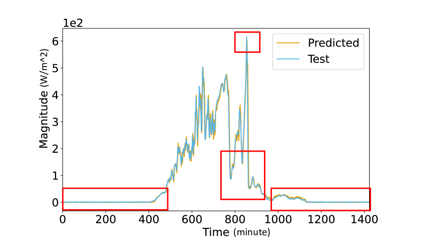
Figure 2: LRNN (top) and ICLRNN (bottom) performances with layer size of (256, 256) on 2023-12-28 for solar irradiance prediction.

IV-C MPC for Continuous Stirred Tank Reactor

MPC is a real-time optimization-based control scheme, where the first element of the optimal input trajectory will be executed in the system over the next sampling period, and the MPC optimization problem will be resolved at the subsequent sampling period iteratively until convergence.

Note that in general, solving NN-MPC is time-consuming, since it is a non-convex optimization problem due to the nonlinearity and nonconvexity of neural network models. However, if we integrate an ICNN into a convex MPC problem, the MPC problem will remain convex. In the next subsection, we will demonstrate the improvement of the computational efficiency of MPC using the proposed ICLRNN in Section III.

IV-C1 Application to a Chemical Process

We implement LMPC to a nonisothermal and well-mixed continuous stirred tank reactor (CSTR) featuring an irreversible second-order exothermic reaction. This reaction facilitates the conversion of reactant A into product B. The CSTR incorporates a heating jacket responsible for either supplying or extracting heat at a rate $Q$. The dynamic model of the CSTR is characterized by the ensuing material and energy balance equations [30, 35]:

$$\frac{dC_{A}}{dt}=\frac{F}{V}(C_{A0}-C_{A})-k_{0}e^{\frac{-E}{RT}}C_{A}^{2}$$ (8a)

$$\frac{dT}{dt}=\frac{F}{V}(T_{0}-T)+\frac{-\triangle H}{\rho_{L}C_{p}}k_{0}e^{\frac{-E}{RT}}C_{A}^{2}+\frac{Q}{\rho_{L}C_{p}V}$$ (8b)

where $C_{A}$ denotes the concentration of reactant A, $F$ denotes the volumetric flow rate, $V$ denotes the volume of the reactant, $C_{A0}$ denotes the inlet concentration of reactant A, $k_{0}$ denotes the pre-exponential constant, $E$ denotes the activation energy, $R$ denotes the ideal gas constant, $T$ denotes the temperature, $T_{0}$ denotes the inlet temperature, $\triangle H$ denotes the enthalpy of reaction, $\rho_{L}$ denotes the constant density of the reactant, $C_{p}$ denotes the heat capacity, and $Q$ denotes the heat input rate. The detailed constant values and system setup are discussed in [30, 35], and are omitted here.

Moreover, $\triangle Q=Q-Q_{s}$ and $\triangle C_{A0}=C_{A0}-C_{A0_{s}}$ denote the manipulated inputs within this system, representing the alterations in the heat input rate and the inlet concentration of reactant A respectively. $x^{T}=[C_{A}-C_{As},T-T_{s}]$ denotes the system states, where $T-T_{s}$ and $C_{A}-C_{As}$ represent the deviations in the temperature of the reactor and the concentration of A from their respective steady-state values. $u^{T}=[\triangle C_{A0},\triangle Q]$ denotes the control actions. The primary objective of the controller involves operating the CSTR at $(C_{As},T_{s})$, which is the unstable equilibrium point, by manipulating $\triangle Q$ and $\triangle C_{A0}$ respectively. This manipulation is executed via the LMPC strategy outlined in Eq. (7) by ultimately stabilizing the state at its target steady-state.

We conduct open-loop simulations for the CSTR of Eq. (8). These simulations aim to collect data that mimics the real-world data for training purposes (i.e., as it is difficult to obtain real-world chemical plant data). All models undergo training and evaluation using uniform configurations, incorporating the Categorical Cross-entropy Loss, the Adam Optimizer, and the ReLU activation function except for LRNN. These models adopt a batch size of 256 and retain a learning rate of 0.001. The LMPC reaches the convergence state when $|x_{1}|=|C_{A}-C_{As}|<0.1\leavevmode\nobreak\ kmol/m^{3}$ and $|x_{2}|=|T-T_{s}|<3\leavevmode\nobreak\ K$ simultaneously. The initial conditions are chosen within the stability region, which is defined as $1060x_{1}^{2}+44x_{1}x_{2}+0.52x_{2}^{2}-372=0$ (i.e., an ellipse in state space). For a comprehensive evaluation of model performance across various hypothesis space sizes and initial conditions, detailed outcomes and discussions are presented in Appendix C.

IV-C2 Computational Efficiency Analysis

To compare the computational efficiency in modeling the system dynamics in Eq. (8) across models, we quantify their FLOPs. Table III illustrates that ICLRNN has the lowest FLOPs, thereby outperforming or matching state-of-the-art methods. Similarly to the results shown in previous tasks, despite LRNN having a relatively modest count of trainable parameters, its high FLOPs indicate substantial computational demands. Conversely, ICRNN encounters challenges with vanishing or exploding gradients, particularly when the network complexity exceeds a certain threshold.

Table III: Model complexity with layer size of (256, 256) for CSTR.

Model	Trainable Parameters	FLOPs
RNN	198,658	406,548
LSTM	793,090	1,597,460
ICRNN	596,482	1,204,233
LRNN	329,730	2,505,748
ICLRNN (ours)	198,658	406,548

IV-C3 Adversarial Robustness Analysis

To scrutinize the adversarial robustness of ICLRNN in modeling the system dynamics in Eq. (8), we assess the model’s sensitivity with respect to test accuracy when exposed to a series of perturbed inputs influenced by Gaussian noise. As illustrated in Fig. 9 detailed in Appendix C, the findings reveal that ICLRNN consistently outperforms or matches the performance of state-of-the-art models across varying levels of noise.

IV-C4 Computational Efficiency of ICLRNN-based LMPC

Incorporating an ICNN into the aforementioned LMPC in Eq. (7) transforms it into a convex optimization problem. Subsequently, PyIpopt, as a Python version of IPOPT [36], is used to address the LMPC problem. The integration time step is set at $h_{c}=10^{-4}\leavevmode\nobreak\ hr$, while the sampling period remains $\triangle=0.005\leavevmode\nobreak\ hr$. The design of the Lyapunov function, denoted as $V(x)=x^{T}Px$, involves configuring the positive definite matrix $P$ as $\big{[}\begin{smallmatrix}1060&22\\ 22&0.52\end{smallmatrix}\big{]}$, which ensures the convexity of the LMPC.

We execute LMPC for a fixed time frame for various models and repeat with various initial conditions to evaluate the performance of different NN-based LMPC. By examining Fig. 3, it is evident that the ICLRNN-based LMPC converges, whereas other NN-based LMPC models do not. The fastest convergence speed highlights the superior computational efficiency of the ICLRNN-based LMPC.

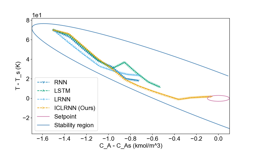
Figure 3: LMPC converging path in a fixed time with an initial condition at $[-1.5\leavevmode\nobreak\ kmol/m^{3},70\leavevmode\nobreak\ K]$.

V Conclusion

This work introduces an Input Convex Lipschitz RNN to improve computational efficiency and adversarial robustness of neural networks in various engineering applications such as image classification, real-world solar irradiance prediction, process modeling and optimization. Theoretical analyses of its input convexity and Lipschitz continuity properties are provided. Additionally, through three case studies, we note that LRNN demanded substantial computational resources, while ICRNN encountered challenges associated with vanishing or exploding gradient problems when operating within large hypothesis space sizes. The ICLRNN model was demonstrated to surpass state-of-the-art recurrent units across various engineering tasks, ranging from simulated studies to real-world applications.

Appendix A MNIST Results

Fig. 4 portrays the testing accuracy of the model in response to varying degrees of Salt and Pepper noise applied to the input. The top left, top right, bottom left, and bottom right figures correspond to model performances with layer sizes of (64, 64), (128, 128), (256, 256), and (512, 512), respectively. These results reveal that, despite different hypothesis space sizes, the testing accuracy of ICLRNN remains consistently superior in handling varied levels of Salt and Pepper noise, showcasing its robustness in adversarial scenarios. Furthermore, ICLRNN exhibits notable computational efficiency, as evidenced by its minimal number of Floating Point Operations (FLOPs) across various hypothesis space sizes.

Moreover, it is important to note that when employing an ICRNN with an extensive hypothesis space size, specifically utilizing more than 128 hidden neurons per layer, it becomes vulnerable to the issue of the exploding gradient problem. This challenge significantly compromises its ability to accurately represent complex system dynamics during the modeling process. Additionally, the FLOPs for LRNN are substantially high, which indicates that it is computationally expensive (i.e., 2,512,956 for LRNN compared to 413,756 for ICLRNN).

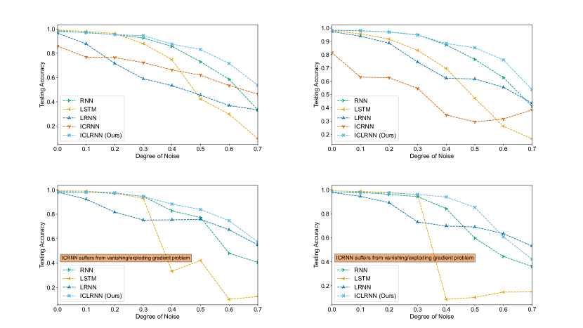
Figure 4: Model performance with layer size of (64, 64), (128, 128), (256, 256), and (512, 512) respectively w.r.t different degree of Salt and Pepper noise for MNIST.

Appendix B Real-World Solar Irradiance Prediction Results

Fig. 5 illustrates the production pipeline adopted by LHT Holdings. Meanwhile, in Fig. 6, a depiction of the different energy sources employed within the production process is presented. Fig. 7 showcases the physical setup of the Solar PV system, encompassing solar panels, inverters, batteries, meters, humidity and wind sensors, module temperature sensors, and irradiance sensors. Data is systematically recorded on a minute-by-minute basis and seamlessly uploaded online into the system.

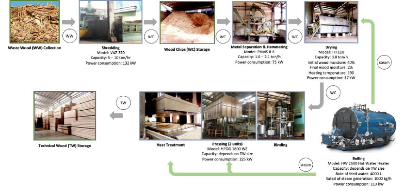
Figure 5: LHT Holdings technical wood production pipeline.

Figure 6: LHT Holdings energy sources for manufacturing.

Figure 7: LHT Holdings Solar PV system.

Fig. 8 shows the model performance on solar irradiance prediction on December 28, 2023. The top two figures display the RNN and LSTM prediction outcomes, respectively. Both models demonstrate poor performance, failing to adjust adequately when faced with sudden changes in solar irradiance, leading to overshooting. Moreover, the middle two figures reveal that the ICRNN encounters issues related to the exploding gradient problem, particularly when the hypothesis space size becomes excessively large. The middle left figure shows the prediction performance of ICRNN with 128 hidden neurons per layer, while the middle right figure shows the prediction performance of ICRNN with 256 hidden neurons per layer. When surpassing 128 hidden neurons per layer, the ICRNN struggles to effectively capture and learn the system’s dynamics.

Moving to the bottom two figures, the LRNN and ICLRNN prediction results for the same date, December 28, 2023, are presented. The LRNN, constrained by Lipschitz continuity, exhibits significantly improved performance compared to the RNN and LSTM models. However, it still encounters challenges in accurately predicting solar irradiance during sudden fluctuations, and its excessively high FLOPs signify its computational intensity (i.e., 2,498,562 for LRNN compared to 399,362 for ICLRNN). Moreover, slight fluctuations in the LRNN predictions occur during periods of minimal solar irradiance at the start and end of the day. Notably, these observations persist across all trials and are not specific solely to December 28, 2023. It is clearly shown in Fig. 2 that our ICLRNN model surpasses state-of-the-art models, demonstrating superior predictive capabilities across various scenarios.

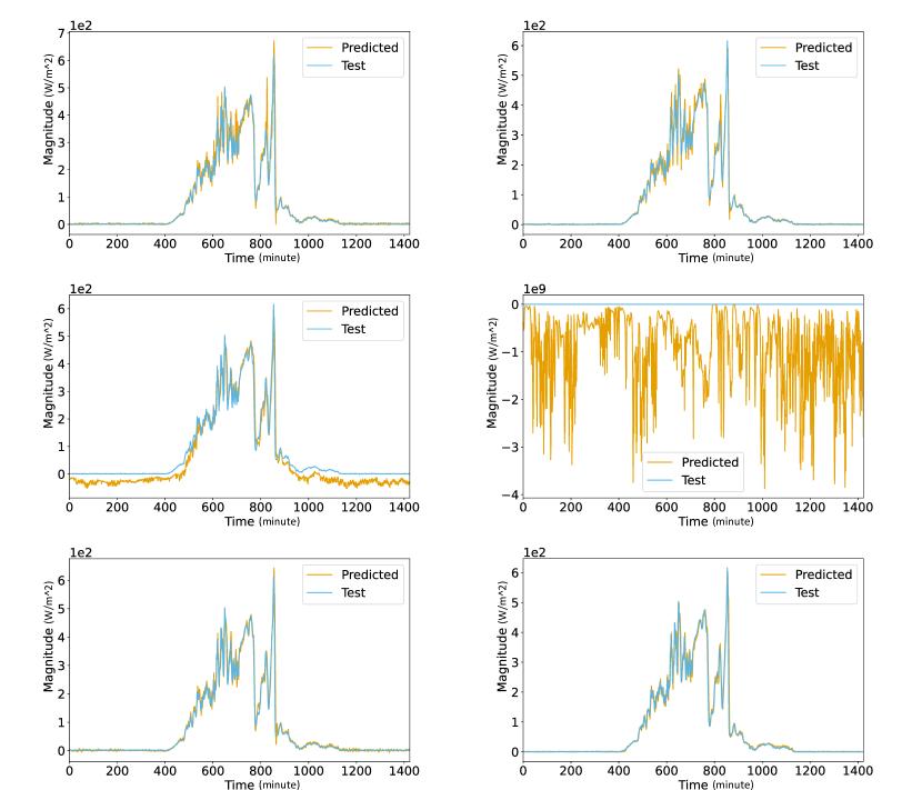
Figure 8: RNN (top left), LSTM (top right), ICRNN (middle left and middle right), LRNN (bottom left), and ICLRNN (bottom right) performance on 2023-12-28 for solar irradiance prediction.

Appendix C MPC-based CSTR Results

Fig. 9 showcases the model’s testing accuracy with respect to varying degrees of Gaussian noise applied to the input. Each quadrant—top left, top right, bottom left, and bottom right—represents the model’s performance with layer sizes of (64, 64), (128, 128), (256, 256), and (512, 512), respectively. These findings indicate ICLRNN’s remarkable adversarial robustness across diverse hypothesis space sizes with respect to different Gaussian noise levels. Notably, ICLRNN exhibits superior computational efficiency, as evidenced by its notably lower number of FLOPs compared to other models.

While ICRNN performs well against various degrees of Gaussian noise within smaller hypothesis spaces, it encounters challenges when the hypothesis space expands, succumbing to the issue of the exploding gradient problem, as evidenced in previous tasks. LRNN demonstrates comparable performance to ICLRNN specifically with a layer size of (512, 512). However, it is computationally demanding, characterized by substantially higher FLOPs (i.e., 9,992,212 for LRNN compared to 1,599,508 for ICLRNN). This computational intensity stands as a significant drawback despite its competitive performance.

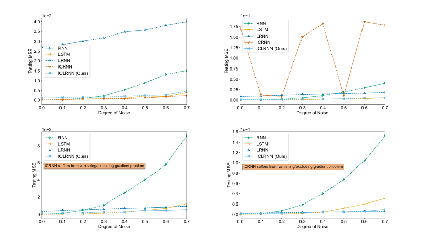
Figure 9: Model performance with layer size of (64, 64), (128, 128), (256, 256), and (512, 512) respectively, w.r.t different degree of Gaussian noise for CSTR.

We now delve into the control performance assessment of NN-based LMPC. To assess and compare the convergence rates of various NN-based LMPC, we conduct different NN-based LMPC under a fixed time frame and repeat with different initial conditions. Figs. 10 and 11 provide compelling evidence that the ICLRNN-based LMPC achieves convergence, unlike other NN-based LMPC, within a fixed time frame. This outcome distinctly indicates that ICLRNN-based LMPC exhibits the fastest convergence speed under identical settings.

In Fig. 10, the left panels show the results corresponding to the initial condition set at $[-1.5\leavevmode\nobreak\ kmol/m^{3},70\leavevmode\nobreak\ K]$. Specifically, the top left panel displays the concentration profile, the middle left panel shows the temperature, and the bottom left panel exhibits the converging path. Additionally, the right panels showcase the results from the initial condition at $[1.5\leavevmode\nobreak\ kmol/m^{3},-70\leavevmode\nobreak\ K]$, featuring the concentration profile in the top right panel, temperature profile in the middle right panel, and the converging path in the bottom right panel. Moving to Fig. 11, the left panels depict the results obtained from the initial condition of $[-1.25\leavevmode\nobreak\ kmol/m^{3},50\leavevmode\nobreak\ K]$. Here, the top left panel represents the concentration, the middle left panel illustrates the temperature, and the bottom left panel shows the converging path. Similarly, the right panels exhibit the results of the initial condition at $[1.25\leavevmode\nobreak\ kmol/m^{3},-50\leavevmode\nobreak\ K]$.

Across various initial conditions, ICLRNN-based LMPC consistently demonstrates the fastest convergence speed, thereby surpassing the state-of-the-art methodologies.

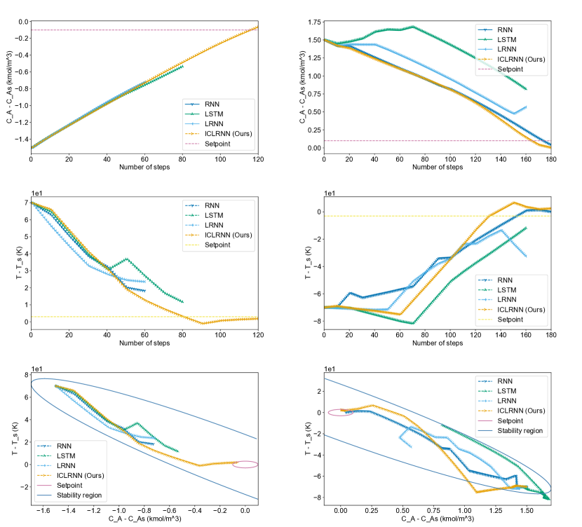
Figure 10: Concentration profile (top left), temperature profile (middle left), converging path (bottom left) in a fixed time with an initial condition at $[-1.5\leavevmode\nobreak\ kmol/m^{3},70\leavevmode\nobreak\ K]$ under LMPC, and concentration profile (top right), temperature profile (middle right), converging path (bottom right) in a fixed time with an initial condition at $[1.5\leavevmode\nobreak\ kmol/m^{3},-70\leavevmode\nobreak\ K]$.

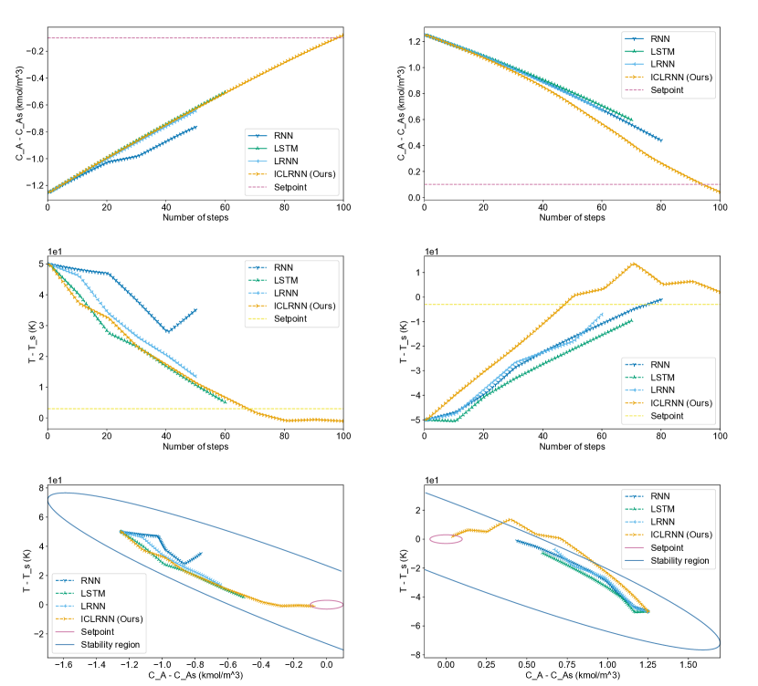
Figure 11: Concentration profile (top left), temperature profile (middle left), converging path (bottom left) in a fixed time with an initial condition at $[-1.25\leavevmode\nobreak\ kmol/m^{3},50\leavevmode\nobreak\ K]$, and concentration profile (top right), temperature profile (middle right), converging path (bottom right) in a fixed time with an initial condition at $[1.25\leavevmode\nobreak\ kmol/m^{3},-50\leavevmode\nobreak\ K]$.

References

- [1] X. Bao, Z. Sun, and N. Sharma, “A Recurrent Neural Network Based MPC for a Hybrid Neuroprosthesis System,” in 2017 IEEE 56th Annual Conference on Decision and Control (CDC), pp. 4715–4720, IEEE, 2017.
- [2] A. Afram, F. Janabi-Sharifi, A. S. Fung, and K. Raahemifar, “Artificial Neural Network (ANN) Based Model Predictive Control (MPC) and Optimization of HVAC Systems: A State of the Art Review and Case Study of a Residential HVAC System,” Energy and Buildings, vol. 141, pp. 96–113, 2017.
- [3] N. Lanzetti, Y. Z. Lian, A. Cortinovis, L. Dominguez, M. Mercangöz, and C. Jones, “Recurrent Neural Network Based MPC for Process Industries,” in 2019 18th European Control Conference (ECC), pp. 1005–1010, IEEE, 2019.
- [4] M. J. Ellis and V. Chinde, “An Encoder-Decoder LSTM-Based EMPC Framework Applied to a Building HVAC System,” Chemical Engineering Research and Design, vol. 160, pp. 508–520, 2020.
- [5] J. Nubert, J. Köhler, V. Berenz, F. Allgöwer, and S. Trimpe, “Safe and Fast Tracking on a Robot Manipulator: Robust MPC and Neural Network Control,” IEEE Robotics and Automation Letters, vol. 5, no. 2, pp. 3050–3057, 2020.
- [6] Y. Zheng, X. Wang, and Z. Wu, “Machine Learning Modeling and Predictive Control of the Batch Crystallization Process,” Industrial & Engineering Chemistry Research, vol. 61, no. 16, pp. 5578–5592, 2022.
- [7] Y. Zheng, T. Zhao, X. Wang, and Z. Wu, “Online Learning-Based Predictive Control of Crystallization Processes under Batch-to-Batch Parametric Drift,” AIChE Journal, vol. 68, no. 11, p. e17815, 2022.
- [8] N. Sitapure and J. S.-I. Kwon, “Neural Network-Based Model Predictive Control for Thin-film Chemical Deposition of Quantum Dots using Data from a Multiscale Simulation,” Chemical Engineering Research and Design, vol. 183, pp. 595–607, 2022.
- [9] Z. Wang and Z. Wu, “Input Convex LSTM: A Convex Approach for Fast Lyapunov-Based Model Predictive Control,” arXiv preprint arXiv:2311.07202, 2023.
- [10] W. G. Y. Tan and Z. Wu, “Robust Machine Learning Modeling for Predictive Control using Lipschitz-Constrained Neural Networks,” Computers & Chemical Engineering, vol. 180, p. 108466, 2024.
- [11] H. Goldstein, C. Poole, and J. Safko, “Classical Mechanics,” 2002.
- [12] J. R. Taylor and J. R. Taylor, Classical Mechanics, vol. 1. Springer, 2005.
- [13] E. M. Purcell, “Electricity and Magnetism,” Berkeley University, vol. 2, 1963.
- [14] D. J. Griffiths, “Introduction to Electrodynamics,” 2005.
- [15] J. B. Hartle, “Gravity: an Introduction to Einstein’s General Relativity,” 2003.
- [16] B. Amos, L. Xu, and J. Z. Kolter, “Input Convex Neural Networks,” in International Conference on Machine Learning, pp. 146–155, PMLR, 2017.
- [17] Y. Chen, Y. Shi, and B. Zhang, “Optimal Control via Neural Networks: A Convex Approach,” arXiv preprint arXiv:1805.11835, 2018.
- [18] C. Anil, J. Lucas, and R. Grosse, “Sorting out Lipschitz Function Approximation,” in International Conference on Machine Learning, pp. 291–301, PMLR, 2019.
- [19] N. B. Erichson, O. Azencot, A. Queiruga, L. Hodgkinson, and M. W. Mahoney, “Lipschitz Recurrent Neural Networks,” arXiv preprint arXiv:2006.12070, 2020.
- [20] M. Serrurier, F. Mamalet, A. González-Sanz, T. Boissin, J.-M. Loubes, and E. Del Barrio, “Achieving Robustness in Classification using Optimal Transport with Hinge Regularization,” in Proceedings of the IEEE/CVF Conference on Computer Vision and Pattern Recognition, pp. 505–514, 2021.
- [21] Y. LeCun, C. Cortes, and C. Burges, “Mnist Handwritten Digit Database,” ATT Labs [Online]. Available: http://yann.lecun.com/exdb/mnist, vol. 2, 2010.
- [22] T. Miyato, T. Kataoka, M. Koyama, and Y. Yoshida, “Spectral Normalization for Generative Adversarial Networks,” arXiv preprint arXiv:1802.05957, 2018.
- [23] G. H. Golub and H. A. Van der Vorst, “Eigenvalue Computation in the 20th Century,” Journal of Computational and Applied Mathematics, vol. 123, no. 1-2, pp. 35–65, 2000.
- [24] Å. Björck and C. Bowie, “An Iterative Algorithm for Computing the Best Estimate of an Orthogonal Matrix,” SIAM Journal on Numerical Analysis, vol. 8, no. 2, pp. 358–364, 1971.
- [25] S. M. Rump, “Verified Bounds for Singular Values, in particular for the Spectral Norm of a Matrix and Its Inverse,” BIT Numerical Mathematics, vol. 51, pp. 367–384, 2011.
- [26] K. Eriksson, D. Estep, and C. Johnson, Applied Mathematics: Body and Soul: Volume 1: Derivatives and Geometry in IR3. Springer Science & Business Media, 2013.
- [27] B. Gao and L. Pavel, “On the Properties of the Softmax Function with Application in Game Theory and Reinforcement Learning,” arXiv preprint arXiv:1704.00805, 2017.
- [28] A. Virmaux and K. Scaman, “Lipschitz Regularity of Deep Neural Networks: Analysis and Efficient Estimation,” Advances in Neural Information Processing Systems, vol. 31, 2018.
- [29] S. P. Boyd and L. Vandenberghe, Convex Optimization. Cambridge University Press, 2004.
- [30] Z. Wu, A. Tran, D. Rincon, and P. D. Christofides, “Machine-Learning-Based Predictive Control of Nonlinear Processes. Part i: Theory,” AIChE Journal, vol. 65, no. 11, p. e16729, 2019.
- [31] Q. V. Le, N. Jaitly, and G. E. Hinton, “A Simple Way to Initialize Recurrent Networks of Rectified Linear Units,” arXiv preprint arXiv:1504.00941, 2015.
- [32] D. P. Kingma and J. Ba, “Adam: A Method for Stochastic Optimization,” arXiv preprint arXiv:1412.6980, 2014.
- [33] V. Nair and G. E. Hinton, “Rectified Linear Units Improve Restricted Boltzmann Machines,” in Proceedings of the 27th international conference on machine learning (ICML-10), pp. 807–814, 2010.
- [34] E. Zelikman, S. Zhou, J. Irvin, C. Raterink, H. Sheng, A. Avati, J. Kelly, R. Rajagopal, A. Y. Ng, and D. Gagne, “Short-Term Solar Irradiance Forecasting using Calibrated Probabilistic Models,” arXiv preprint arXiv:2010.04715, 2020.
- [35] Z. Wu, A. Tran, D. Rincon, and P. D. Christofides, “Machine-Learning-Based Predictive Control of Nonlinear Processes. Part ii: Computational Implementation,” AIChE Journal, vol. 65, no. 11, p. e16734, 2019.
- [36] A. Wächter and L. T. Biegler, “On the Implementation of an Interior-Point FilterLine-Search Algorithm for Large-Scale Nonlinear Programming,” Mathematical programming, vol. 106, pp. 25–57, 2006.