USTC-ICTS/PCFT-24-02

Partial entanglement network and bulk geometry reconstruction in AdS/CFT

Abstract

In the context of Anti-de Sitter / Conformal Field Theory (AdS/CFT) correspondence, we present a general scheme to reconstruct bulk geometric quantities in terms of a specific measure of the entanglement structure on the boundary CFT, the partial entanglement entropy (PEE). The PEE between any two points $\mathcal{I}(\textbf{x},\textbf{y})$ is the fundamental building block of the PEE structure. It can be geometrized into a bulk geodesic connecting the two boundary points x and y, which we refer to as the PEE thread. Thus, we have a network of the PEE threads in the bulk with a density of the threads determined by the boundary PEE structure [1]. We demonstrate that, for any static boundary region $A$, the homologous surface $\Sigma_{A}$ that has the minimal flux of the PEE threads passing through it is exactly the Ryu-Takayanagi (RT) surface of $A$, and the minimal flux coincides with the holographic entanglement entropy of $A$. Furthermore, we show that the strength of the PEE flux at any bulk point along any direction is $1/4G$. Based on this observation, we prove that any area element in the bulk can be reconstructed by the PEE threads passing through it, which corresponds to a set of two-point PEEs on the CFT.

Introduction – The AdS/CFT correspondence [2, 3, 4] states that the quantum theory of gravity in asymptotic AdS_d+1 spacetime is equivalent to a certain CFT_d on the asymptotic boundary. This provides a window to understand both of the classical and quantum aspects of the theory of gravity based on the information in the boundary CFT, using the dictionary of the correspondence. Several important developments have been made along this line [5, 6, 7, 8, 9, 10, 11], where the insights from a holographic perspective of boundary quantum entanglement structure have played a central role. These achievements began with the Ryu-Takayanagi (RT) formula [5] which relates the entanglement entropy of any boundary region to the area of the bulk minimal surface homologous to that boundary region. This proposal was later refined to the covariant version [6, 11] and the version including quantum corrections [7, 8, 9, 10]. For more recent developments on the bulk reconstruction inspired by holographic study of quantum entanglement, one should consult the following review papers [12, 13].

In this paper, we focus on the reconstruction of bulk geometric quantities in terms of boundary entanglement structure measures. So far, several approaches have been explored for this goal. For example, the reconstruction of certain bulk curves via the differential entropy [14, 15, 16, 17, 18, 19] by studying the geodesics tangent to the curve, the reformulation of the RT formula as the maximal flux of the bit threads in AdS space out of the region [20, 21, 22], and the simulation of the AdS space based on the tensor networks [23, 24, 25, 26, 27, 28, 29, 30] where the RT surface is interpreted as the homologous path in the network with the minimal number of cut. See [31] for a detailed review on the above approaches. Nevertheless, the geometry reconstruction program is far from complete. Inspired by these approaches, we propose a framework to reconstruct all the bulk geometric quantities based on a new measure of entanglement, the partial entanglement entropy (PEE) [32, 33, 34, 35, 36]. See [37, 38, 39, 40, 41, 42, 43, 44, 45, 46] for discussions on the relation between PEE and the above three approaches, and see also [47, 48, 49, 50, 51, 52] for the reconstruction of the entanglement wedge cross-section in various scenarios based on PEE.

The partial entanglement network – The PEE $\mathcal{I}(A,B)$ is a special measure of two-body correlation between two non-overlapping regions $A$ and $B$ [32, 33, 35, 36]. The PEE not only satisfies all the properties of the mutual information, but also the additional key property of additivity [53, 33],

$$\mathcal{I}(A,B\cup C)=\mathcal{I}(A,B)+\mathcal{I}(A,C)\,.$$ (1)

Given the additivity and the property of $\mathcal{I}(A,B)=\mathcal{I}(B,A)$, the PEE can always be decomposed into a summation of the two-point PEEs,

$$\mathcal{I}(A,B)=\int_{A}\mathrm{d}^{d-1}\textbf{x}\int_{B}\mathrm{d}^{d-1}\textbf{y}~{}\mathcal{I}(\textbf{x},\textbf{y})\,.$$ (2)

In the vacuum state of a CFT_d, these requirements determine the formula of the PEE [33, 1] (see also [54, 55] for related discussion),

$$\mathcal{I}(\textbf{x},\textbf{y})=\frac{c}{6}\frac{2^{d-1}(d-1)}{\Omega_{d-2}|\textbf{x}-\textbf{y}|^{2(d-1)}},$$ (3)

where $\Omega_{d-2}={2\pi^{\frac{d-1}{2}}}/{\Gamma\left(\frac{d-1}{2}\right)}$ is the area of $(d-2)$-dimensional unit sphere. The normalization property of the PEE $\mathcal{I}(A,B)|_{B\to\bar{A}}=S_{A}$ tells us how to approach the entanglement entropy from PEE,

$$S_{A}=\int_{A}\mathrm{d}^{d-1}\textbf{x}\int_{\bar{A}-\epsilon}\mathrm{d}^{d-1}\textbf{y}~{}\mathcal{I}(\textbf{x},\textbf{y}),$$ (4)

where $A\cup\bar{A}$ makes a pure state and $\epsilon$ represent a regularization. This requirement is subtle since entanglement entropy is divergent and depends on the regularization scheme in quantum field theories. Nevertheless, in CFT_d entanglement entropies for various shapes of connected regions have been carried out based on (3) and (4) [56, 57, 58, 59], which are in good agreement with the results derived from other methods . Although the PEE structure (3) may not capture all the information of the entanglement structure in a CFT, we will see that it is enough to reconstruct the geometry in the gravity dual in AdS/CFT.

In AdS/CFT, we introduced a scheme to geometrize the PEEs in [1], where the boundary two-point PEEs $\mathcal{I}(\textbf{x},\textbf{y})$ are represented by the bulk geodesics connecting the two boundary points $\{\textbf{x},\textbf{y}\}$, which we call the PEE threads [1]. We only consider the vacuum state of the CFT_d and a time slice in AdS_d+1. The PEE threads emanating from any point x can be represented by a divergenceless vector field $V_{\textbf{x}}^{\mu}=|V_{\textbf{x}}|\tau^{\mu}$, where $\tau^{\mu}$ is the unite vector tangent to the geodesics emanating from x. The norm $|V_{\textbf{x}}|$ characterizes the density of the threads, which is determined by the requirement that, the flux of the PEE threads from x to any boundary region $\mathrm{d}\sigma$ should match the PEE $\mathcal{I}(\textbf{x},\mathrm{d}\sigma)$. In summary, given the PEE structure of the boundary CFT and the metric of the dual spacetime, we get a network of the PEE threads in the AdS bulk consisting of all the bulk geodesics anchored on the boundary (see Fig. 1 for examples). We call it the partial entanglement network, or PEE network for short. In poincaré AdS_d+1 with unit AdS radius,

$$\mathrm{d}s^{2}=\frac{-\mathrm{d}t^{2}+\mathrm{d}z^{2}+\mathrm{d}r^{2}+r^{2}\mathrm{d}\Omega_{d-2}^{2}}{z^{2}},$$ (5)

the vector field that describes the PEE threads emanating from the origin was carried out in [1],

$$V_{O}(Q)=\frac{2^{d}z^{d}}{4G}\frac{(d-1)}{\Omega_{d-2}}\frac{r}{(r^{2}+z^{2})^{d}}\left(z,\frac{z^{2}-r^{2}}{2r},0,\cdots\right)\,,$$ (6)

where $Q=({z},{r},\phi_{i},\dots)$ is any point in the bulk. The $V_{O}^{\phi_{i}}$ components are zero due to the rotation symmetry. See a brief derivation of (6) in the Supplementary Material. Moreover, the vector flow from any boundary point x is identical to (6) up to a translation.

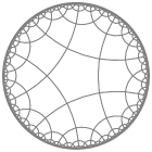
Figure 1: Visualizations of PEE threads (gray) on a time slice of Poincaré AdS₄ and global AdS₃, where the boundary sites (on the plane) are discretized. Left: the PEE threads with larger radii are denoted with thinner curves, whose thickness reflects the density of the PEE threads. Right: with appropriate discretizations, they form a hyperbolic tiling.

Then the calculation of the entanglement entropy (4) for an arbitrary region $A$ has a corresponding picture in the partial entanglement network. This equates to calculating the flux of the PEE thread flow from $A$ to $\bar{A}$ [1]. More explicitly, we first do a summation for all the PEE flow $V_{\textbf{x}}^{\mu}$ with $\textbf{x}\in A$ to get a total vector flow $V_{A}^{\mu}=\int_{A}\mathrm{d}^{d-1}\textbf{x}V_{\textbf{x}}^{\mu}$, then the flux out of $A$ is given by

$$S_{A}=\int_{\Sigma_{A}}\mathrm{d}\Sigma_{A}\sqrt{h}V_{A}^{\mu}n_{\mu},$$ (7)

where $\Sigma_{A}$ is any co-dimensional two surface homologous to $A$, $n^{\mu}$ is the outward normal unite vector and $h$ is the induced metric. This flux is independent of the choice of $\Sigma_{A}$ as $V_{A}^{\mu}$ is divergenceless. Naively, we expect that (7) should reproduce the same entanglement entropy as the RT formula. Indeed, for the particular choices of static spherical regions, we set $\Sigma_{A}$ as the RT surface, and then the flow $V_{A}^{\mu}$ comes out orthogonally and has a norm $\frac{1}{4G}$, which is exactly a bit thread [20] configuration constructed in [61]. Then the total flux out of $A$ (7) is just $\frac{\mathrm{Area}[\Sigma_{A}]}{4G}$ [1], which aligns with the RT formula. However, this coincidence does not happen for other regions, see [1] for case of a strip region.

Figure 2: Here $A=A_{1}\cup A_{2}$, $\bar{A}=\bar{A}_{1}\cup\bar{A}_{2}$ and $A\bar{A}$ is in the vacuum state of the holographic CFT₂. Representative PEE threads (dashed curves) in Poincaré AdS₃. Each PEE thread crosses the disconnected RT surface with different times, corresponding to different weights.

To fix this problem, we should modify (4) in some way. The discussion for the two-interval case in [1] in CFT₂ provides a clear clue. Let us consider a two interval $A=A_{1}\cup A_{2}$ whose RT surface is given by the blue curves, see Fig. 2. If we naively apply (4), we should only count the threads connecting $A_{i}$ and $\bar{A}_{j}$, which gives $S_{A}=\mathcal{I}(A_{1},\bar{A})+\mathcal{I}(A_{2},\bar{A})$. On the other hand, the RT formula implies

$$S_{A}= S_{A_{1}}+S_{A_{2}}=\mathcal{I}(A_{1},A_{2}\bar{A})+\mathcal{I}(A_{2},A_{1}\bar{A})$$ (8)

$$= \mathcal{I}(A_{1},\bar{A})+\mathcal{I}(A_{2},\bar{A})+2\mathcal{I}(A_{1},A_{2})\,,$$ (9)

where we used (4) for $A_{1}$ and $A_{2}$ as it applies to single intervals. The RT formula not only counts the threads connecting $A$ and $\bar{A}$, but also doubly counts the threads connecting $A_{1}$ and $A_{2}$. This absolutely goes beyond (4), but looks reasonable as the threads connecting $A_{1}$ and $A_{2}$ intersect with the RT surface twice. Then one may weight the threads with the number it intersects with the RT surface. For any disjoint multi-interval $A=\cup A_{i}$ and its complement $\bar{A}=\cup\bar{A}_{j}$, given the RT surface we can read the weight for any PEE threads. Let us denote the weight for the threads connecting any two sub-intervals $\alpha$ and $\beta$ as $\omega(\alpha,\beta)$. It has further been checked in [1] that the holographic entanglement entropy is given by

$$S_{A}=\sum_{i,j}\big{(}\omega(A_{i},A_{j})\mathcal{I}(A_{i} ,A_{j})+\omega(\bar{A}_{i},\bar{A}_{j})\mathcal{I}(\bar{A}_{i},\bar{A}_{j})$$ (10)

$$+\omega(A_{i},\bar{A}_{j})\mathcal{I}(A_{i},\bar{A}_{j})\big{)}\,.$$ (11)

The above observation is consistent with (4) for single interval cases where only the threads connecting the interval $A$ and its complement $\bar{A}$ have non-zero weight $\omega(A,\bar{A})=1$. From bulk PEE flux perspective, it is important to note that, (10) indeed computes the PEE flux that flows from the entanglement wedge $\mathcal{W}_{A}$ to $\mathcal{W}_{\bar{A}}$, instead of the flux from $A$ to $\bar{A}$.

Reformulation of the RT formula– Now we extend to general dimensional Poincaré AdS_d+1 and get rid of the precondition that we know the RT surface. For any disconnected boundary region $A=\cup A_{i}$ and its compliment $\bar{A}=\cup\bar{A}_{j}$, we consider an arbitrary co-dimension two surface $\Sigma_{A}$ homologous to $A$. If we define the weight of a PEE thread as the number it intersects with the surface $\Sigma_{A}$, then the configuration of the weights depends on $\Sigma_{A}$. In higher dimensions, PEE threads that anchored on the same connected subregion $A_{i}$ can pass through the RT surface hence has non-zero weight (see Fig. 3 for the example of a strip region). So, when we talk about the weight of a PEE thread, we should also specify the two boundary points it connects. For these reasons, we denote the weight of the thread connecting the pair of the boundary points $\{\textbf{x},\textbf{y}\}$ as $\omega_{\Sigma_{A}}(\textbf{x},\textbf{y})$. We do not need to count the threads tangent to $\Sigma_{A}$.

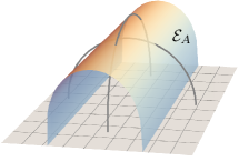
Figure 3: The RT surface $\mathcal{E}_{A}$ for a strip region $A$ in Poincaré AdS₄. The PEE threads (the gray curves) with both endpoints inside or outside $A$ can possibly pass through $\mathcal{E}_{A}$ twice.

Inspired by the above observation (10), here we give a proposal as a complete reformulation of the RT formula. Given a homologous surface $\Sigma_{A}$, it always divides the bulk space $\mathcal{M}$ into two parts $\mathcal{M}_{A}$ and $\mathcal{M}_{\bar{A}}$ whose boundaries satisfy

$$\partial\mathcal{M}_{A}=A\cup\Sigma_{A}\,,\qquad\partial\mathcal{M}_{\bar{A}}=\bar{A}\cup\Sigma_{A}\,.$$ (12)

We propose that, the $\Sigma_{A}$ that minimizes the PEE flux from $\mathcal{M}_{A}$ to $\mathcal{M}_{\bar{A}}$ is exactly the RT surface, and the corresponding minimal flux coincides with the holographic entanglement entropy, i.e.

$$S_{A}=\min_{\Sigma_{A}}\frac{1}{2}\int_{\partial\mathcal{M}}\mathrm{d}^{d-1}\textbf{x}\int_{\partial\mathcal{M}}\mathrm{d}^{d-1}\textbf{y}~{}\omega_{\Sigma_{A}}(\textbf{x},\textbf{y})\mathcal{I}(\textbf{x},\textbf{y}),$$ (13)

where the integration domain of x and y is the whole AdS boundary $\partial\mathcal{M}=A\bar{A}$. Here we have considered all the PEE threads and their weights instead of only those connecting $A$ and $\bar{A}$. The factor $1/2$ appears as we count both $\mathcal{I}(\textbf{x},\textbf{y})$ and $\mathcal{I}(\textbf{y},\textbf{x})$ in the integration. The above equation can also be written in terms of the PEE vector flows

$$S_{A}=\min_{\Sigma_{A}}~{}\frac{1}{2}\int_{\Sigma_{A}}\mathrm{d}\Sigma_{A}\sqrt{h}\int_{\partial\mathcal{M}}\mathrm{d}^{d-1}\textbf{x}|V_{\textbf{x}}^{\mu}n_{\mu}|.$$ (14)

Similarly, the coefficient $1/2$ appears because we integrate x over the whole boundary such that the PEE thread connecting any two boundary point is doubly counted. Here we take the absolute value for $V_{\textbf{x}}^{\mu}n_{\mu}$ since locally we are always calculating the flow from one side of $\Sigma_{A}$ to the other side, hence any PEE thread passing through $\Sigma_{A}$ gives positive contribution.

The version of the above proposal in AdS₃/CFT₂ was proposed and tested in [1] without proof. In the following we present simple and general proof for any static boundary region $A$ in AdS_d+1/CFT_d. This proposal gives a complete reformulation of the RT formula, as the minimization reproduces the RT surface, and the minimized flux reproduces the holographic entanglement entropy.

Figure 4: Representative PEE threads in Poincaré AdS₃. The blue shaded region is the entanglement wedge $\mathcal{W}_{A}$ of $A$. PEE threads that pass through a surface segment $\mathrm{d}\mathcal{E}_{A}$ of the RT surface are denoted by gray solid curves, among which the green solid curve represents the shortest one. PEE threads that do not intersect $\mathrm{d}\mathcal{E}_{A}$ are denoted by gray dashed curves.

Proof– Although the analysis of the PEE flow for static spherical regions [1] looks quite special, it contains the key ingredient to prove our proposal for generic regions. Consider a spherical region $A$. Its RT surface $\mathcal{E}_{A}$ is just a hemisphere, and the PEE threads can be classified into three classes,

1. $\omega_{\mathcal{E}_{A}}(\textbf{x},\textbf{y})=0$ for $\textbf{x},\textbf{y}\in A$;

2. $\omega_{\mathcal{E}_{A}}(\textbf{x},\textbf{y})=0$ for $\textbf{x},\textbf{y}\in\bar{A}$;

3. $\omega_{\mathcal{E}_{A}}(\textbf{x},\textbf{y})=1$ for $\textbf{x}\in A,\textbf{y}\in\bar{A}$ or $\textbf{x}\in\bar{A},\textbf{y}\in A$.

Only the third class of threads intersects with $\mathcal{E}_{A}$. More specifically, let us consider an infinitesimal area element $\sqrt{h}\mathrm{d}\mathcal{E}_{A}$ on the RT surface. It is obvious that the gray curves (as well as a green curve) emanating from $A$ (see Fig. 4) represent all the threads that pass through $\sqrt{h}\mathrm{d}\mathcal{E}_{A}$. So we only need to integrate the PEE flow $V_{\textbf{x}}^{\mu}$ for $x\in A$ to get flux of PEE threads out of the area element, which is just [1]

$$\sqrt{h}\mathrm{d}\mathcal{E}_{A}\int_{A}\mathrm{d}\textbf{x}~{}V_{\textbf{x}}^{\mu}n_{\mu}=\frac{\sqrt{h}\mathrm{d}\mathcal{E}_{A}}{4G}\,.$$ (15)

See a brief derivation of (15) in the Supplementary Material. We can conclude that, for any area element on the RT surface of any static spherical region, the density of the PEE flux passing through this area element is exactly $1/4G$.

Figure 5: Here $\Sigma$ represents an arbitrary codimension-2 bulk curve in AdS₃. Any infinitesimal line segment at $Q_{i}$ is reconstructed by the set of PEE threads passing through it and emanating from the spherical region whose RT surface (gray dashed line) is tangent to $\Sigma$ at $Q_{i}$.

Then we consider an arbitrary area element at a bulk point $Q$ with a unit normal vector $n^{\mu}(Q)$. It is crucial to notice that, any area element can be embedded on a unique RT surface $\mathcal{E}_{A}$ of a spherical region $A$, where $\mathcal{E}_{A}$ is the hemisphere passing through $Q$ and normal to $n^{\mu}(Q)$ (see Fig. 5 for the cases of infinitesimal line segments in AdS₃). Then we can calculate the PEE flux of this area element by just collecting the threads emanating from the corresponding spherical region $A$. Remarkably, according to our discussion for the spherical regions, we conclude that the density of the PEE flux through an arbitrary area element is $1/4G$, i.e. at any point $Q$ for any $n^{\mu}$ we always have

$$\int_{A}\mathrm{d}^{d-1}\textbf{x}|V_{\textbf{x}}^{\mu}n_{\mu}|=\frac{1}{2}\int_{\partial\mathcal{M}}\mathrm{d}^{d-1}\textbf{x}|V_{\textbf{x}}^{\mu}n_{\mu}|=\frac{1}{4G}\,.$$ (16)

Here we have used the fact that, the PEE threads emanating from $\bar{A}$ and passing through $Q$ are exactly those emanating from the spherical region $A$.

Now we consider an arbitrary co-dimension two surface $\Sigma_{A}$ in the AdS bulk homologous to any boundary region $A$, and divide $\Sigma_{A}$ into infinitesimal area elements. At this point, we are ready to prove our proposal (14) by applying the above conclusion to all the area elements on $\Sigma_{A}$, so we have

$$S_{A}= \frac{1}{4G}\min_{\Sigma_{A}}~{}\int_{\Sigma_{A}}\mathrm{d}\Sigma_{A}\sqrt{h}$$ (17)

$$= \min_{\Sigma_{A}}\frac{\mathrm{Area}[\Sigma_{A}]}{4G}=\frac{\mathrm{Area}[\mathcal{E}_{A}]}{4G}\,,$$ (18)

which is exactly the RT formula.

Bulk geometry reconstruction– Our goal is to interpret all the geometric quantities in terms of the boundary PEEs. We just interpreted the RT surfaces as the homologous surface that minimizes the flux of the PEE flow from $\mathcal{M}_{A}$ to $\mathcal{M}_{\bar{A}}$, and the minimized flux gives the area of the RT surface. In other words, we reconstructed all the RT surfaces via the class of PEE threads passing through it.

Similarly, we can reconstruct an arbitrary infinitesimal bulk co-dimension two surface $\mathrm{d}\Sigma$ from certain class of boundary two-point PEEs $\mathcal{I}(\textbf{x},\textbf{y})$, whose PEE threads pass through $\mathrm{d}\Sigma$. According to our previous discussion, the class of PEE threads that pass $\mathrm{d}\Sigma$ are those emanating from a spherical region whose RT surface is tangent to $\mathrm{d}\Sigma$, and the flux of the PEE flow passing through $\mathrm{d}\Sigma$ gives $\text{Area}(\mathrm{d}\Sigma)$,

$$\frac{\mathrm{Area}(\mathrm{d}\Sigma)}{4G}= \frac{1}{2}\int_{{\partial\mathcal{M}}}\mathrm{d}^{d-1}\textbf{x}\int_{\partial\mathcal{M}}\mathrm{d}^{d-1}\textbf{y}~{}\omega_{\mathrm{d}\Sigma}(\textbf{x},\textbf{y})\mathcal{I}(\textbf{x},\textbf{y})\,,$$ (19)

where $\omega_{\mathrm{d}\Sigma}(\textbf{x},\textbf{y})=0$ or $1$ depending on whether the thread intersects with $\mathrm{d}\Sigma$. The PEE threads that do not intersect with $\mathrm{d}\Sigma$ will not participate on its reconstruction.

Interestingly, given the position of a $\mathrm{d}\Sigma$, the scale $|\textbf{x}-\textbf{y}|$ of all the two-point PEEs $\mathcal{I}(\textbf{x},\textbf{y})$ that participate in the reconstruction of $\mathrm{d}\Sigma$, is lower bounded. For example, in Poincaré AdS_d+1, the scale of those two-point PEEs satisfy

$$|\textbf{x}-\textbf{y}|\geq 2z_{0},$$ (20)

where $z_{0}$ is the $z$ coordinate of $\mathrm{d}\Sigma$. In other words, the two-point PEEs with $|\textbf{x}-\textbf{y}|<2z_{0}$ will not contribute to the reconstruction of area elements deeper than $z_{0}$. See Fig. 6 for two examples in global AdS₃, where we show the set of PEE threads that reconstruct two different area elements. In the left case, the $\mathrm{d}\Sigma$ is close to the boundary, hence the small scale PEEs contribute. In the right case, the $\mathrm{d}\Sigma$ is in the center of the AdS space and only the largest scale PEEs involve in its reconstruction.

Figure 6: The area element $\mathrm{d}\Sigma$ and its direction is represented by the black arrow. The gray curves represent all the PEE threads that involve in the reconstruction of $\mathrm{d}\Sigma$, and the green curve represents the PEE thread that saturates the lower bound.

We can also reconstruct any co-dimension two surface $\Sigma$ in the bulk, which does not need to be homologous to any boundary region. Because we can reconstruct all the infinitesimal area elements on the surface, see Fig. 5. Then all the PEEs that locally pass through $\Sigma$ will contribute to the reconstruction. And the area of $\Sigma$ will be reproduced by the flux locally passing through it, which is just

$$\frac{\mathrm{Area}(\Sigma)}{4G}= \frac{1}{2}\int_{{\partial\mathcal{M}}}\mathrm{d}^{d-1}\textbf{x}\int_{\partial\mathcal{M}}\mathrm{d}^{d-1}\textbf{y}~{}\omega_{\Sigma}(\textbf{x},\textbf{y})\mathcal{I}(\textbf{x},\textbf{y})\,.$$ (21)

Discussion– In summary, based on the PEE structure of a CFT and its geometrization scheme represented by all the geodesics anchored on the boundary, we obtain a network of geodesics which could be considered as the basic elements forming the AdS space in AdS/CFT. We show that the strength of the PEE flow at any bulk point in any direction is always $1/4G$, which means that the AdS space is full of PEE threads. Then any geometric quantity in AdS can be reconstructed by a set of boundary PEEs with their PEE threads passing through it. And we abandon the naive normalization property (4) of the PEE.

We also provide a complete reformulation of the RT formula, which aims to identify the homologous surface $\Sigma_{A}$ with minimal PEE flux. This is partially inspired by the evaluation of the entanglement entropy of CFT₂ in the model of tensor networks, where the homologous path has the minimal number of cuts with the network. Here the PEE network is analogous to the tensor network, and the PEE flux through the homologous surface is akin to the number of cuts the surface intersects with the PEE network.

It is intriguing to view the PEE network as the tensor network which precisely captures the entanglement structure of the boundary CFT at large $c$ limit. Compared with previous tensor network toy models of gravity, the PEE network is a well-defined continuous network that naturally extends to higher dimensions. It will be interesting to add bulk degrees of freedom to the PEE network, to study the quantum correction and quantum error correction property of the PEE network. Extending or testing our scheme to more generic asymptotic AdS spacetimes, to the covariant configurations and to holographies beyond AdS/CFT are also worth exploring.

Acknowledgements– Y. Lu is supported by the National Natural Science Foundation of China under Grant No.12247161, the NSFC Research Fund for International Scientists (Grant No. 12250410250) and China Postdoctoral Science Foundation under Grant No.2022TQ0140. J. Lin is supported by the National Natural Science Foundation of China under Grant No.12247117, No.12247103. Q. Wen would like to thank Bartlomiej Czech, Veronika E. Hubeny, Ling-Yan Hung, Huajia Wang and Zhenbin Yang for helpful discussions.

Supplementary Materials

Appendix A The derivation of the PEE threads flow

Figure 7: Determine the PEE thread flow $V^{\mu}_{O}$ at the point $Q=(r,z)$ by letting the flux of the PEE threads (the red curves) through the reference RT surface $\Sigma$ (the blue semicircle) with the radius $\ell=\sqrt{r^{2}+z^{2}}$ being equal to the entanglement contour of $r=0$ to the region $[-\ell,\ell]$

In this appendix, we present a brief derivation of the vector flow $V_{O}(Q)$ (6) that describes all the PEE threads emanating from the origin point $O$. In higher dimensions, due to the rotational symmetry of $V_{O}$, we can restrict to a 2-dimensional slice with $\phi_{i}=0$. Since the PEE threads are just the bulk geodesics emanating from $O$, $V_{O}(Q)$ is tangent to these geodesics, such that

$$V_{O}^{\mu}(Q)=|V_{O}(Q)|\tau_{O}^{\mu}(Q),$$ (22)

where

$$\tau_{O}^{\mu}(Q)=\frac{2zr}{r^{2}+z^{2}}\left(z,\frac{z^{2}-r^{2}}{2r}\right),$$ (23)

is the unit tangent vector to the PEE threads, $z$ and $r$ are the coordinates of $Q$. The norm $|V_{O}(Q)|$ is then settled down by the requirement that, the flux of the PEE threads from the origin to any boundary region $\mathrm{d}y$ should match the PEE $y^{d-2}\mathcal{I}(0,\mathrm{d}y)$. Explicitly, let us consider a reference RT surface $\Sigma$ passing through $Q$ with the radius $\ell=\sqrt{r^{2}+z^{2}}$ (see Fig. 7). The flux of the PEE threads $V_{O}^{\mu}$ through an area element $\mathrm{d}\Sigma$ on $\Sigma$ is given by

$$\text{Flux}(V_{O}^{\mu},\mathrm{d}\Sigma)= \mathrm{d}\theta\sqrt{h_{\theta\theta}}V_{O}^{\mu}(\theta)n_{\Sigma,\mu}$$ (24)

$$= \mathrm{d}\theta\sqrt{h_{\theta\theta}}|V_{O}(\theta)|\sin\theta,$$

where $\theta=\arctan\frac{z}{r}$, $h_{\theta\theta}=1/\sin^{2}\theta$ is the $\theta\theta$-component of the induced metric on $\Sigma$ and $n_{\Sigma}^{\mu}(Q)=\ell\sin\theta(\cos\theta,\sin\theta)$ is the unit normal vector on $\Sigma$. Then solving

$$\text{Flux}(V_{O}^{\mu},\mathrm{d}\Sigma)=y^{d-2}\mathcal{I}(0,\mathrm{d}y)=\mathrm{d}y~{}y^{d-2}\mathcal{I}(0,y),\ y=\ell/\cos\theta,$$ (25)

the norm is given by

$$|V_{O}(Q)|=\frac{1}{4G}\frac{2^{d-1}(d-1)}{\Omega_{d-2}}\frac{z^{d-1}}{(r^{2}+z^{2})^{d-1}}.$$ (26)

Finally, we obtain the PEE threads flow

$$V_{O}(Q)=\frac{2^{d}z^{d}}{4G}\frac{(d-1)}{\Omega_{d-2}}\frac{r}{(r^{2}+z^{2})^{d}}\left(z,\frac{z^{2}-r^{2}}{2r},0,\cdots\right)\,.$$ (27)

Appendix B The flux of the PEE threads flow in AdS₃

Now let us give a brief derivation on the flux of the PEE threads flow emanating from a connected region $A=[-R,R]$ and through an infinitesimal area element $\sqrt{h}\mathrm{d}\mathcal{E}_{A}$ on the RT surface of $A$. Due to shift symmetry along $r$-direction in AdS₃, the PEE thread flow with $r=r_{0}$ can be obtained by replacing $r$ with $r-r_{0}$ in (27) and

$$V_{r_{0}}^{\mu}=\frac{1}{4G}\frac{2z^{2}(r-r_{0})}{((r-r_{0})^{2}+z^{2})^{2}}\left(z,\frac{z^{2}-(r-r_{0})^{2}}{2(r-r_{0})}\right).$$ (28)

Then the flux of all the PEE thread flow $V_{r_{0}}^{\mu}$ emanating from the points inside $A$ and through $\mathrm{d}\mathcal{E}_{A}$ is given by

$$\text{Flux}(V_{r_{0}}^{\mu},\mathrm{d}\mathcal{E}_{A}) =\sqrt{h}\mathrm{d}\mathcal{E}_{A}\int^{R}_{-R}\mathrm{d}r_{0}V_{r_{0}}^{\mu}n_{\mu}=\frac{\sqrt{h}\mathrm{d}\mathcal{E}_{A}}{4G},$$ (29)

where $n^{\mu}=z(\frac{r}{R},\frac{z}{R})$ is the unit normal vector on the RT surface of $A$. Note that although the above derivation is restricted to AdS₃ cases, the result of the flux (29) actually holds for general dimensions with the spherical region $A$. One may consult [1] for the details.

References

- Lin et al. [2023a] J. Lin, Y. Lu, and Q. Wen, Geometrizing the Partial Entanglement Entropy: from PEE Threads to Bit Threads, (2023a), arXiv:2311.02301 [hep-th] .
- Maldacena [1998] J. M. Maldacena, The Large N limit of superconformal field theories and supergravity, Adv. Theor. Math. Phys. 2, 231 (1998), arXiv:hep-th/9711200 .
- Gubser et al. [1998] S. S. Gubser, I. R. Klebanov, and A. M. Polyakov, Gauge theory correlators from noncritical string theory, Phys. Lett. B 428, 105 (1998), arXiv:hep-th/9802109 .
- Witten [1998] E. Witten, Anti-de Sitter space and holography, Adv. Theor. Math. Phys. 2, 253 (1998), arXiv:hep-th/9802150 .
- Ryu and Takayanagi [2006] S. Ryu and T. Takayanagi, Holographic derivation of entanglement entropy from AdS/CFT, Phys. Rev. Lett. 96, 181602 (2006), arXiv:hep-th/0603001 .
- Hubeny et al. [2007] V. E. Hubeny, M. Rangamani, and T. Takayanagi, A Covariant holographic entanglement entropy proposal, JHEP 07, 062, arXiv:0705.0016 [hep-th] .
- Lewkowycz and Maldacena [2013] A. Lewkowycz and J. Maldacena, Generalized gravitational entropy, JHEP 08, 090, arXiv:1304.4926 [hep-th] .
- Faulkner et al. [2013] T. Faulkner, A. Lewkowycz, and J. Maldacena, Quantum corrections to holographic entanglement entropy, JHEP 11, 074, arXiv:1307.2892 [hep-th] .
- Engelhardt and Wall [2015] N. Engelhardt and A. C. Wall, Quantum Extremal Surfaces: Holographic Entanglement Entropy beyond the Classical Regime, JHEP 01, 073, arXiv:1408.3203 [hep-th] .
- Dong [2014] X. Dong, Holographic Entanglement Entropy for General Higher Derivative Gravity, JHEP 01, 044, arXiv:1310.5713 [hep-th] .
- Dong et al. [2016] X. Dong, A. Lewkowycz, and M. Rangamani, Deriving covariant holographic entanglement, JHEP 11, 028, arXiv:1607.07506 [hep-th] .
- Bousso et al. [2022] R. Bousso, X. Dong, N. Engelhardt, T. Faulkner, T. Hartman, S. H. Shenker, and D. Stanford, Snowmass White Paper: Quantum Aspects of Black Holes and the Emergence of Spacetime, (2022), arXiv:2201.03096 [hep-th] .
- Faulkner et al. [2022] T. Faulkner, T. Hartman, M. Headrick, M. Rangamani, and B. Swingle, Snowmass white paper: Quantum information in quantum field theory and quantum gravity, in Snowmass 2021 (2022) arXiv:2203.07117 [hep-th] .
- Balasubramanian et al. [2014] V. Balasubramanian, B. D. Chowdhury, B. Czech, J. de Boer, and M. P. Heller, Bulk curves from boundary data in holography, Phys. Rev. D 89, 086004 (2014), arXiv:1310.4204 [hep-th] .
- Headrick et al. [2014] M. Headrick, R. C. Myers, and J. Wien, Holographic Holes and Differential Entropy, JHEP 10, 149, arXiv:1408.4770 [hep-th] .
- Czech et al. [2014] B. Czech, X. Dong, and J. Sully, Holographic Reconstruction of General Bulk Surfaces, JHEP 11, 015, arXiv:1406.4889 [hep-th] .
- Czech and Lamprou [2014] B. Czech and L. Lamprou, Holographic definition of points and distances, Phys. Rev. D 90, 106005 (2014), arXiv:1409.4473 [hep-th] .
- Czech et al. [2015] B. Czech, L. Lamprou, S. McCandlish, and J. Sully, Integral Geometry and Holography, JHEP 10, 175, arXiv:1505.05515 [hep-th] .
- Czech et al. [2016] B. Czech, L. Lamprou, S. McCandlish, and J. Sully, Tensor Networks from Kinematic Space, JHEP 07, 100, arXiv:1512.01548 [hep-th] .
- Freedman and Headrick [2017] M. Freedman and M. Headrick, Bit threads and holographic entanglement, Commun. Math. Phys. 352, 407 (2017), arXiv:1604.00354 [hep-th] .
- Headrick et al. [2022] M. Headrick, J. Held, and J. Herman, Crossing Versus Locking: Bit Threads and Continuum Multiflows, Commun. Math. Phys. 396, 265 (2022), arXiv:2008.03197 [hep-th] .
- Headrick and Hubeny [2023] M. Headrick and V. E. Hubeny, Covariant bit threads, JHEP 07, 180, arXiv:2208.10507 [hep-th] .
- Swingle [2012a] B. Swingle, Entanglement Renormalization and Holography, Phys. Rev. D 86, 065007 (2012a), arXiv:0905.1317 [cond-mat.str-el] .
- Evenbly and Vidal [2011] G. Evenbly and G. Vidal, Tensor network states and geometry, J. Stat. Phys. 145, 891 (2011), arXiv:1106.1082 [quant-ph] .
- Swingle [2012b] B. Swingle, Constructing holographic spacetimes using entanglement renormalization, (2012b), arXiv:1209.3304 [hep-th] .
- Qi [2013] X.-L. Qi, Exact holographic mapping and emergent space-time geometry, (2013), arXiv:1309.6282 [hep-th] .
- Pastawski et al. [2015] F. Pastawski, B. Yoshida, D. Harlow, and J. Preskill, Holographic quantum error-correcting codes: Toy models for the bulk/boundary correspondence, JHEP 06, 149, arXiv:1503.06237 [hep-th] .
- Hayden et al. [2016] P. Hayden, S. Nezami, X.-L. Qi, N. Thomas, M. Walter, and Z. Yang, Holographic duality from random tensor networks, JHEP 11, 009, arXiv:1601.01694 [hep-th] .
- Bhattacharyya et al. [2016] A. Bhattacharyya, Z.-S. Gao, L.-Y. Hung, and S.-N. Liu, Exploring the Tensor Networks/AdS Correspondence, JHEP 08, 086, arXiv:1606.00621 [hep-th] .
- Bhattacharyya et al. [2018] A. Bhattacharyya, L.-Y. Hung, Y. Lei, and W. Li, Tensor network and (-adic) AdS/CFT, JHEP 01, 139, arXiv:1703.05445 [hep-th] .
- Chen et al. [2022] B. Chen, B. Czech, and Z.-z. Wang, Quantum information in holographic duality, Rept. Prog. Phys. 85, 046001 (2022), arXiv:2108.09188 [hep-th] .
- Wen [2018] Q. Wen, Fine structure in holographic entanglement and entanglement contour, Phys. Rev. D 98, 106004 (2018), arXiv:1803.05552 [hep-th] .
- Wen [2020a] Q. Wen, Formulas for Partial Entanglement Entropy, Phys. Rev. Res. 2, 023170 (2020a), arXiv:1910.10978 [hep-th] .
- Wen [2020b] Q. Wen, Entanglement contour and modular flow from subset entanglement entropies, JHEP 05, 018, arXiv:1902.06905 [hep-th] .
- Han and Wen [2022] M. Han and Q. Wen, Entanglement entropy from entanglement contour: higher dimensions, SciPost Phys. Core 5, 020 (2022), arXiv:1905.05522 [hep-th] .
- Han and Wen [2021] M. Han and Q. Wen, First law and quantum correction for holographic entanglement contour, SciPost Phys. 11, 058 (2021), arXiv:2106.12397 [hep-th] .
- Kudler-Flam et al. [2019] J. Kudler-Flam, I. MacCormack, and S. Ryu, Holographic entanglement contour, bit threads, and the entanglement tsunami, J. Phys. A 52, 325401 (2019), arXiv:1902.04654 [hep-th] .
- Wen [2019] Q. Wen, Towards the generalized gravitational entropy for spacetimes with non-Lorentz invariant duals, JHEP 01, 220, arXiv:1810.11756 [hep-th] .
- Abt et al. [2019] R. Abt, J. Erdmenger, M. Gerbershagen, C. M. Melby-Thompson, and C. Northe, Holographic Subregion Complexity from Kinematic Space, JHEP 01, 012, arXiv:1805.10298 [hep-th] .
- Rolph [2022] A. Rolph, Local measures of entanglement in black holes and CFTs, SciPost Phys. 12, 079 (2022), arXiv:2107.11385 [hep-th] .
- Gong et al. [2023] A. Gong, C.-B. Chen, and F.-W. Shu, Kinematic space for quantum extremal surface, (2023), arXiv:2305.15885 [hep-th] .
- Lin et al. [2022] Y.-Y. Lin, J.-R. Sun, Y. Sun, and J.-C. Jin, The PEE aspects of entanglement islands from bit threads, JHEP 07, 009, arXiv:2203.03111 [hep-th] .
- Lin et al. [2021] Y.-Y. Lin, J.-R. Sun, and J. Zhang, Deriving the PEE proposal from the locking bit thread configuration, JHEP 10, 164, arXiv:2105.09176 [hep-th] .
- Lin and Zhang [2023] Y.-Y. Lin and J. Zhang, Holographic coarse-grained states and the necessity of perfect entanglement, (2023), arXiv:2312.14498 [hep-th] .
- Lin et al. [2023b] Y.-Y. Lin, J. Zhang, and J.-C. Jin, Entanglement islands read perfect-tensor entanglement, (2023b), arXiv:2312.14486 [hep-th] .
- Lin [2023] Y.-Y. Lin, Distilled density matrices of holographic partial entanglement entropy from thread-state correspondence, Phys. Rev. D 108, 106010 (2023), arXiv:2305.02895 [hep-th] .
- Wen [2021] Q. Wen, Balanced Partial Entanglement and the Entanglement Wedge Cross Section, JHEP 04, 301, arXiv:2103.00415 [hep-th] .
- Camargo et al. [2022] H. A. Camargo, P. Nandy, Q. Wen, and H. Zhong, Balanced partial entanglement and mixed state correlations, SciPost Phys. 12, 137 (2022), arXiv:2201.13362 [hep-th] .
- Wen and Zhong [2022] Q. Wen and H. Zhong, Covariant entanglement wedge cross-section, balanced partial entanglement and gravitational anomalies, SciPost Phys. 13, 056 (2022), arXiv:2205.10858 [hep-th] .
- Basu [2022] D. Basu, Balanced Partial Entanglement in Flat Holography, (2022), arXiv:2203.05491 [hep-th] .
- Basu et al. [2023] D. Basu, J. Lin, Y. Lu, and Q. Wen, Ownerless island and partial entanglement entropy in island phases, (2023), arXiv:2305.04259 [hep-th] .
- Lin et al. [2023c] J. Lin, Y. Lu, and Q. Wen, Cutoff brane vs the Karch-Randall brane: the fluctuating case, (2023c), arXiv:2312.03531 [hep-th] .
- Chen and Vidal [2014] Y. Chen and G. Vidal, Entanglement contour, Journal of Statistical Mechanics: Theory and Experiment , P10011 (2014), arXiv:1406.1471 [cond-mat.str-el] .
- Casini and Huerta [2009] H. Casini and M. Huerta, Remarks on the entanglement entropy for disconnected regions, JHEP 03, 048, arXiv:0812.1773 [hep-th] .
- Singha Roy et al. [2020] S. Singha Roy, S. N. Santalla, J. Rodríguez-Laguna, and G. Sierra, Entanglement as geometry and flow, Phys. Rev. B 101, 195134 (2020), arXiv:1906.05146 [quant-ph] .
- Bueno et al. [2015a] P. Bueno, R. C. Myers, and W. Witczak-Krempa, Universality of corner entanglement in conformal field theories, Phys. Rev. Lett. 115, 021602 (2015a), arXiv:1505.04804 [hep-th] .
- Bueno et al. [2015b] P. Bueno, R. C. Myers, and W. Witczak-Krempa, Universal corner entanglement from twist operators, JHEP 09, 091, arXiv:1507.06997 [hep-th] .
- Bueno et al. [2019] P. Bueno, H. Casini, and W. Witczak-Krempa, Generalizing the entanglement entropy of singular regions in conformal field theories, JHEP 08, 069, arXiv:1904.11495 [hep-th] .
- Bueno et al. [2021] P. Bueno, H. Casini, O. L. Andino, and J. Moreno, Disks globally maximize the entanglement entropy in 2 + 1 dimensions, JHEP 10, 179, arXiv:2107.12394 [hep-th] .
- Note [1] In these papers, the authors studied the mutual information that satisfies additivity (EMI), which coincides with the PEE [33] in these scenarios. See [33, 35] for discussion on the relationship between the PEE and the EMI.
- Agón et al. [2019] C. A. Agón, J. De Boer, and J. F. Pedraza, Geometric Aspects of Holographic Bit Threads, JHEP 05, 075, arXiv:1811.08879 [hep-th] .