CarSpeedNet: A Deep Neural Network-based Car Speed Estimation from Smartphone Accelerometer

Abstract

In this study, a novel deep neural network (DNN) architecture, CarSpeedNet, is introduced to estimate car speed using three-axis accelerometer data from smartphones. Utilizing 13 hours of data collected from smartphones mounted in cars navigating through various regions in Israel, the CarSpeedNet effectively learns the relationship between measured smartphone acceleration and car speed. Ground truth speed data was obtained at 1[Hz] from the GPS receiver in the smartphones. The proposed model enables high-frequency speed estimation, incorporating historical inputs. Our trained model demonstrates exceptional accuracy in car speed estimation, achieving a precision of less than 0.72[m/s] during an extended driving test, solely relying on smartphone accelerometer data without any connectivity to the car.

I Introduction

In the contemporary landscape of car technology and traffic management, the accurate estimation of car speed is a cornerstone, essential for ensuring road safety, optimizing traffic flow, and enhancing navigational systems [1, 2, 3, 4, 5]. Historically, speed measurement has been primarily reliant on traditional instruments such as the car’s built-in odometer. However, these conventional methods are fraught with limitations, particularly in their connectivity and data-sharing capabilities [6]. This limitation is critical in an era where real-time data and its seamless transmission are indispensable for efficient traffic management and safety applications [7, 8, 9, 10].

As we pivot towards more advanced and universally accessible methodologies, smartphones emerge as a potent tool in this domain [11]. Equipped with an array of sophisticated sensors, notably accelerometers, smartphones present a novel approach to speed estimation. These accelerometers, capable of measuring specific forces along three axes, function at high frequencies — sometimes exceeding 100 [Hz], in certain devices even reaching 500 [Hz]. This high-frequency measurement capability of smartphone accelerometers is pivotal in capturing the nuanced variations in vehicular speed, a critical factor in the accurate estimation of car dynamics under diverse driving conditions.

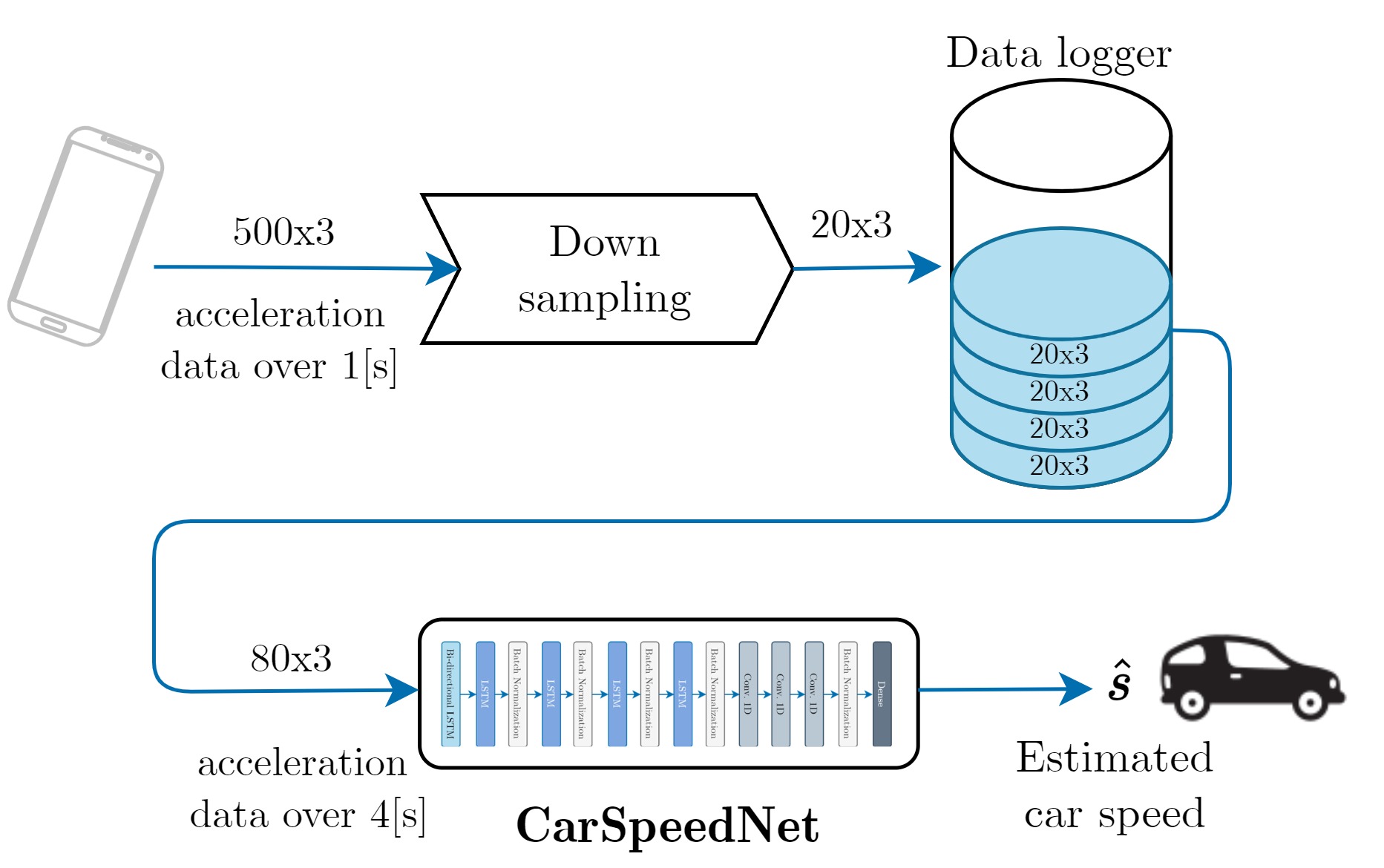
Figure 1: A diagram of the suggested approach in this work: smartphone accelerometer data is processed, including downsampling and batch aggregation. The final step involves inputting this prepared data into CarSpeedNet to accurately estimate the car’s speed.

Despite their ubiquity and advanced sensor technology, the use of smartphones for car speed estimation is not without challenges. One of these is the transformation of raw accelerometer data into accurate and reliable speed estimates. This translation requires sophisticated data processing and analysis methods, an area where deep learning algorithms excel [12].

Deep Neural Networks (DNNs), a class of machine learning models inspired by the neural networks of the human brain, have shown significant promise in extracting meaningful patterns from large datasets [13]. Their ability to learn complex relationships within data makes them particularly suited for applications like speed estimation from accelerometer data. The burgeoning field of deep learning in car technology is an area ripe for exploration, offering the potential to revolutionize traditional speed estimation methods [14, 15, 16].

In this study, we introduce a novel deep neural network architecture, CarSpeedNet, designed specifically to harness the data from smartphone accelerometers for car speed estimation. The uniqueness of this research lies in its singular focus on accelerometer data, bypassing the need for other sensors like gyroscopes, which, while beneficial, do not universally exist in all smartphones, as explored in previous works [2, 17, 18, 19]. This approach ensures that our solution is accessible to a broad user base, regardless of their device’s specific hardware capabilities.

The need for a solution that is not only accurate but also universally accessible is at the heart of this research. By focusing exclusively on accelerometer data, we aim to democratize access to advanced vehicular speed estimation technologies, ensuring that all drivers, irrespective of their smartphone model, can benefit from this technology.

Moreover, the emphasis on a deep learning approach signifies a paradigm shift from traditional speed estimation methods [18]. By leveraging the prowess of DNNs, we aim to not only match but surpass the accuracy of traditional methods, all while utilizing a sensor that is already widely available in consumer devices.

Our methodology for achieving this involves a two-phase approach: first, the meticulous collection of a comprehensive dataset of acceleration signals from multiple smartphones, and second, the deployment of a supervised learning paradigm for training our DNN model. This data-driven approach is critical in ensuring that the model is not only theoretically but also practically effective under real-world driving conditions.

The methodology scheme is presented in Figure 1 where the smartphone’s accelerometer readings are downsampled and logged to batches of 4 [s] and then forwards into the CarSpeedNet that outputs an estimation for the car’s speed.

The schematic representation of the proposed methodology is illustrated in Figure 1, wherein the accelerometer data from the smartphone undergoes a downsampling process. This data is subsequently aggregated into batches with a duration of 4 [s] each. Following this preparatory step, the aggregated data is input into the CarSpeedNet, output a precise estimation of the car’s speed.

The contributions of this work are:

• Developed CarSpeedNet, a novel deep neural network for estimating car speed using smartphone accelerometer data.

• Demonstrated the ability of DNNs to accurately interpret complex patterns from accelerometer data for precise speed estimation.

• Implemented a comprehensive methodology for data collection and model training, ensuring practical applicability in real-world scenarios.

• Advanced the use of smartphone technology in traffic management and safety, offering a universally accessible alternative to traditional car-based systems.

The structure of the paper is organized as follows: Section II outlines the learning approach, encompassing aspects such as motivation, data acquisition and database creation, defining the loss function, exploring various models, and culminating in the development of CarSpeedNet. Section III is dedicated to presenting the results and discussion, which includes defining the error metric, conducting a comparative analysis of the model’s performance, and examining the impact of input size on CarSpeedNet’s effectiveness. Finally, Section IV concludes the paper.

II Learning Approach

This section discusses the motivation behind focusing solely on accelerometer data, overcoming challenges associated with noise in these sensors, and the shift from previous methods that included gyroscope measurements. This section also details the process of data acquisition and dataset creation using a Samsung Galaxy Smartphone, emphasizing the importance of precision in ground truth labels from GPS data. Additionally, it explores various deep neural network models, leading to the development of CarSpeedNet, and describes the architecture and training process of this final model.

II-A Motivation

The genesis of this research lies in the quest to refine car speed estimation techniques by exclusively utilizing accelerometer data, a shift from our previous work which incorporated gyroscope measurements. This strategic pivot is motivated by the widespread prevalence of accelerometers in smartphones, whereas gyroscopes are not as universally available. The direct calculation of speed from accelerometer data is notoriously fraught with challenges, predominantly due to the noise inherent in these low-cost sensors. Such noise leads to substantial divergence when the acceleration is integrated to estimate velocity.

In our pursuit to surmount these challenges, we introduce a novel Deep Neural Network (DNN)-based approach for car speed estimation. By harnessing only accelerometer data, we aim to make this solution more accessible and applicable to a wider range of devices. Our approach utilizes a supervised learning paradigm, where the accelerometer data is meticulously labeled with precise speed measurements obtained from the smartphone’s GNSS receiver. This framework empowers the DNN model to accurately predict car speed, effectively mitigating the noise-related limitations of accelerometer data.

II-B Data Acquisition and Dataset Creation

The dataset was meticulously assembled utilizing a Samsung Galaxy Smartphone, equipped with an integrated accelerometer and GPS. The accelerometer data was captured at a high-resolution frequency of 500 [Hz], while the GPS data was recorded at 1 [Hz]. A pivotal aspect of this assembly process was the synchronization of all sensors to a unified time reference, ensuring temporal coherence across the data streams.

In the realm of supervised machine learning, the precision of ground truth labels is paramount. Accordingly, the car speed measurements derived from the GPS data were adopted as the canonical labels for this study.

The comprehensive dataset encapsulates a total of 13.2 hours of vehicular operation, distributed across 51 distinct driving sessions. To evaluate the model’s performance, one driving session, lasting 30 minutes, was exclusively reserved for testing. Consequently, the remaining 50 sessions, accounting for 12.9 hours, were allocated for model training. Further refinement of the training dataset ensued, with an 80:20 division into training (10.3 hours) and validation (2.6 hours) subsets.

The data aggregation was extensively conducted across various geographical terrains within the state of Israel, encompassing an array of road types, predominantly highways and urban streets. It is imperative to note that the data collection was strictly confined to on-road scenarios, deliberately excluding off-road data acquisition. Additionally, the driving sessions were exclusively conducted during daylight hours under standard meteorological conditions, ensuring consistency in environmental factors.

A crucial aspect of the data integrity involved the preliminary stabilization of GPS signals. Each driving session commenced only after attaining a stabilized GPS signal, ascertained through the Global Dilution of Precision (GDOP) metric, thereby minimizing locational inaccuracies [20, 5]. The raw data underwent meticulous processing, where the IMU data was subjected to low-pass filtering to mitigate noise interference and subsequently downsampled to a frequency of 20 [Hz]. Concurrently, the car speed data, ascertained from the GPS readings, was maintained at a consistent recording frequency of 1 [Hz].

II-C Loss Function

The following mean square error (MSE) loss function was minimized in the training stage

$${\cal L}=\frac{1}{{2N}}\sum\limits_{j=1}^{N}{{{\left({{s}_{j}^{GT}-{{{\hat{s}}}_{j}}\left({{\bf{a}};{\bf{W}}}\right)}\right)}^{2}}}$$ (1)

In this equation, $\cal L$ denotes the loss function. The term $\frac{1}{{2N}}$ represents the normalization factor, where $N$ is the total number of samples in the batch. The ${s}_{j}^{GT}$ stands for the ground truth value for the $j^{th}$ sample, and ${{{\hat{s}}}_{j}}\left({{\bf{a}};{\bf{W}}}\right)$ represents the predicted value by the network for the same sample. The prediction is a function of $\bf a$, the input acceleration data, and $\bf W$, the learnable weights of the neural network.

The squared difference quantifies the discrepancy between the predicted value and the actual ground truth. The squaring ensures that larger errors are more heavily penalized, contributing to a more robust model training by emphasizing the reduction of larger prediction errors.

II-D Models Exploration

In our research, we explored various DNN architectures until we found the CarSpeedNet. Each model was carefully selected and tailored to suit the specific requirements of our problem, focusing on the number of trainable parameters, the composition of various layers, and their implications on model performance.

• DNN*: Adopted from previuos work [2]. The architecture comprises one long short-term memory (LSTM) layer [21], two bidirectional LSTM layers [22], and a single dense layer to output the estimated speed. This model boasts a total of 13,031 trainable parameters. Originally designed for processing both accelerometer and gyroscope measurements. we adapted and retrained DNN* exclusively for accelerometer inputs, aligning it with our specific data framework.

• LSTM: Embodies a sequential arrangement of LSTM and Batch Normalization layers, augmented with dropout for regularization. The model structure is as follows: Input layer accommodating the specified sample size and three-dimensional accelerometer data. Multiple LSTM layers with varying units and dropout values. Batch Normalization layers interspersed between LSTM layers. A concluding dense layer with linear activation for speed estimation. This model encompasses 17,181 trainable parameters, indicating a modest complexity while retaining the capacity to capture essential temporal features.

• WaveNet: The waveNet architecture [23], renowned for its proficiency in processing temporal sequence data for the audio domain. The WaveNet model is characterized by a series of convolutional layers with varying dilation rates to capture different temporal scales. Rectifier linear unit (ReLU) activation functions following each convolutional layer, and a final convolutional layer to produce the output. This model is significantly larger, with a total of 239,937 parameters, indicative of its extensive capability to model complex temporal patterns.

• Bi-LSTM: The bi-directional LSTM (Bi-LSTM) model includes an input layer for handling three-dimensional accelerometer data, combination of bidirectional LSTM and standard LSTM layers, incorporating dropout. Finally, a dense output layer. This model has 26,251 trainable parameters, leveraging the strength of bidirectional LSTM layers to capture bidirectional temporal dependencies.

• ResNet-inspired: We experimented with a model inspired by the ResNet architecture [24], renowned for its effectiveness in various DNN applications. It integrates ResNet blocks with Bi-LSTM layers and is characterized by custom ResNet blocks with convolutional, Batch Normalization layers, and Bidirectional LSTM layers for capturing temporal dependencies. The total number of trainable parameters for this model is 95,043.

Through a rigorous process of experimentation and iterative refinement, informed by performance evaluations of various layer configurations, we have converged on an architecture that we designate as CarSpeedNet. This architecture represents the culmination of a systematic trial-and-error approach, where insights gleaned from each iteration have guided the progressive enhancement of the model’s design. The subsequent subsection delves into the intricacies of CarSpeedNet.

II-E The CarSpeedNet

II-E1 Architecture

The CarSpeedNet architecture (shown in Figure 2) is suited for processing data samples that have a shape of $80\times 3$, representing 80 sequential data points along 4[s], each with 3 axes of accelerometer inputs. Following the input layer, the network features a series of recurrent neural layers, specifically Long Short-Term Memory (LSTM) layers. These LSTM layers are effective in capturing long-range dependencies in sequential data.

The network notably includes a bidirectional LSTM with 100 units, capable of processing data in both directions, thereby greatly enhancing the understanding of the data’s context. This is followed by a series of standard LSTM layers, with reduced numbers of units (50, 20, 20, 20), each carefully preserving the sequence of the data.

Between these LSTM layers, Batch Normalization is applied consistently. This approach normalizes the activations from the previous layer in each batch, significantly reducing internal covariate shifts and improving the network’s training speed and stability.

As the network moves past the recurrent layers, it transitions to a convolutional stage, specifically using one-dimensional convolutions (Conv1D). This part of the architecture, comprising three Conv1D layers with 64, 64, and 32 filters each, a kernel size of 3, and ’same’ padding, is designed for effective feature extraction from sequential data. These convolutional layers are each followed by a Rectified Linear Unit (ReLU) activation function, introducing non-linearity to the network and enabling it to learn more complex data patterns.

The architecture reaches its final stage with two fully connected (Dense) layers. The first Dense layer, with 32 units activated by the ReLU function, further processes and interprets the features extracted by previous layers. The concluding layer, a single Dense unit, is the speed estimation output.

The architectural framework of CarSpeedNet is distinguished by its bifurcated structure, systematically designed to address the dual aspects of feature extraction: temporal and spatial.

Initially, the architecture focuses on the extraction of temporal features. This phase is crucial for discerning the sequential dependencies and dynamics inherent in time-series data, such as the accelerometer readings. By effectively capturing these temporal relationships, the model lays the groundwork for a nuanced understanding of the car’s motion over time. Subsequently, the model shifts its focus to the extraction of spatial features from the temporally processed data. This stage is instrumental in identifying and isolating spatial patterns and correlations within the data, which are critical for comprehending the multi-dimensional nature of the accelerometer inputs.

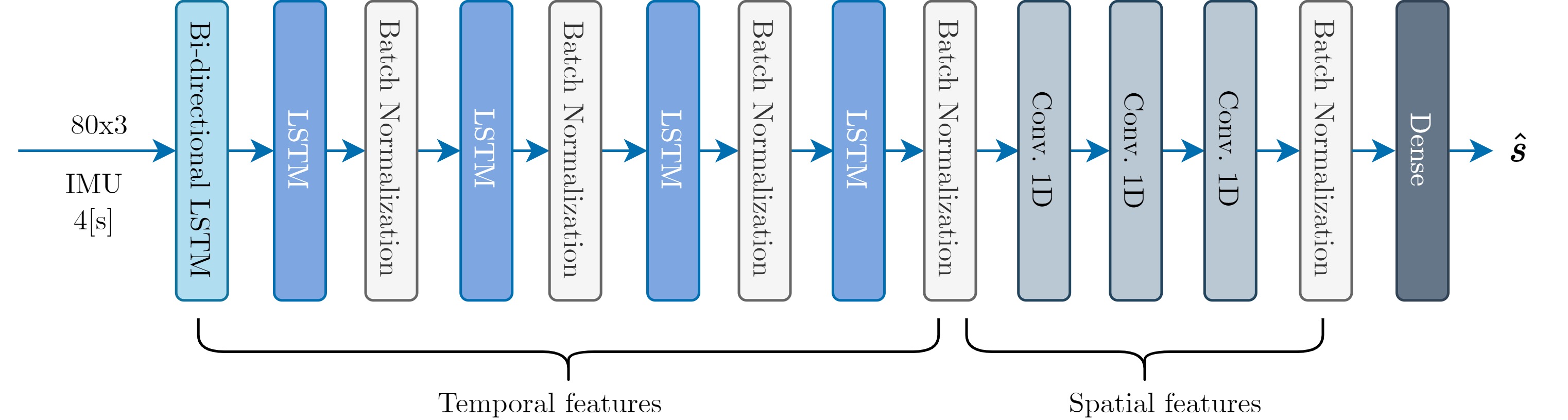
Figure 2: The CarSpeedNet architecture

II-E2 Training

The training process of CarSpeedNet leveraging a total of 178,169 trainable parameters. This substantial number of parameters underpins the model’s capacity to learn complex, high-dimensional mappings from smartphone accelerometer data to speed predictions. The model training commenced with the Adam optimizer [25]. An initial learning rate of 0.001 was set. To enhance the training effectiveness, an exponential decay learning rate schedule was employed. This approach systematically reduces the learning rate over training epochs, starting from the initial rate of 0.001. Specifically, the learning rate was scheduled to decay over 30,000 steps, with a decay rate of 0.2.

A salient feature of the training process was the implementation of early stopping, a regularization technique used to prevent overfitting. Early stopping monitored the validation loss with a patience parameter set to 1000 epochs. The overall training was configured to span a maximum of 200 epochs. However, the incorporation of early stopping provided flexibility, allowing the training to cease earlier if the validation loss plateaued, indicating no further learning progress. This approach not only optimizes computational resources but also safeguards the model against overfitting the training data.

The training process was conducted with a batch size of 32. The outcomes and insights derived from this rigorous training process are thoroughly delineated in the Results and Discussion section.

III Results and Discussion

In this section, we evaluate the performance of our suggested model. We employ two key error metrics to assess the model’s predictive accuracy. Following this, we conduct a comparative analysis of various model architectures, focusing on error metrics, and computational efficiency. Additionally, we explore the impact of varying input sizes on our model’s performance and discuss its real-time applications, emphasizing its adaptability in different scenarios.

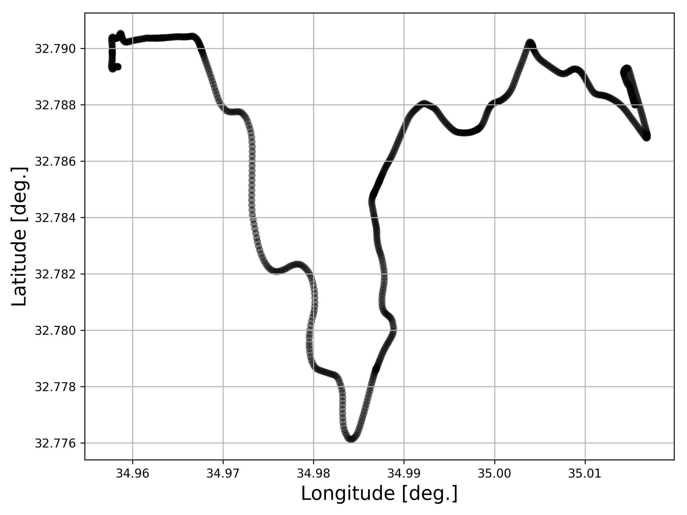
Figure 3: Trajectory of the test drive over 30 minutes.

III-A Error Metrics

For the comprehensive evaluation of the predictive accuracy of our model, two primary error metrics are employed: the Root Mean Square Error (RMSE) and the Mean Absolute Error (MAE). The RMSE is a robust metric that provides a measure of the magnitude of the error. It is particularly sensitive to large errors, making it a reliable indicator of the model’s accuracy. The RMSE is computed as follows:

$$RMSE=\sqrt{\frac{1}{N}\sum\limits_{j=1}^{N}{{{\left({s_{j}^{GT}-{\hat{s}_{j}}}\right)}^{2}}}}$$ (2)

The squaring of the errors before averaging and the subsequent square root transformation ensure that the RMSE is in the same units as the predicted variable, thereby facilitating a more intuitive interpretation of the model’s performance.

The MAE, on the other hand, offers a direct average measure of the absolute discrepancies between the predicted values and the actual values. It is defined as:

$$MAE=\frac{1}{N}\sum\limits_{j=1}^{N}{\left|{s_{j}^{GT}-{\hat{s}_{j}}}\right|}$$ (3)

The MAE is less sensitive to outliers compared to RMSE, providing a straightforward indication of the average error magnitude.

III-B Comparative Analysis of Model Performances

This subsection provides a comparative analysis of the performances of the various models mentioned in section II.D. The evaluation focuses on three pivotal metrics: RMSE and MAE, both measured in m/s units, and the computational time required for processing.

Central to this analysis is Figure 4, which graphically displays the RMSE and MAE values for each model.

All the results in this subsection are computed for 1[s] accelerometer input (20 measurements).

The LSTM model shows commendable predictive accuracy with an RMSE of 4.54 [m/s] and a moderate MAE of 3.06 [m/s]. It has a latency of 104.8 [ms]. In contrast, the WaveNet model, while exhibiting a slightly higher RMSE of 5.7 [m/s] and an MAE of 3.2 [m/s], offers the advantage of lower latency at 63 [ms]. However, this model is characterized by a substantially larger number of trainable parameters (239,937), potentially impacting its computational efficiency. The Bidirectional LSTM model indicates relatively higher prediction errors, with an RMSE of 10.8 [m/s] and an MAE of 8.5 [m/s], coupled with a latency of 93.8 [ms]. This suggests its limited efficacy in capturing the complex dynamics of the data. Remarkably, the ResNet model stands out with its predictive performance, exhibiting a low RMSE of 2.9 [m/s] and a minimal MAE of 1.4 [m/s], alongside a latency of 87.9 [ms]. The DNN* model, adapted from a previous study, demonstrates strong predictive capability with an RMSE of 3.5 [m/s] and a low MAE of 1.9 [m/s]. Latency is 101[ms]. The CarSpeedNet architecture achieves an outstandingly low RMSE of 2.9 [m/s], complemented by a minimal MAE of only 1.3 [m/s]. Furthermore, it maintains a latency of 104.8 [ms], striking a balance between rapid response time and computational efficiency.

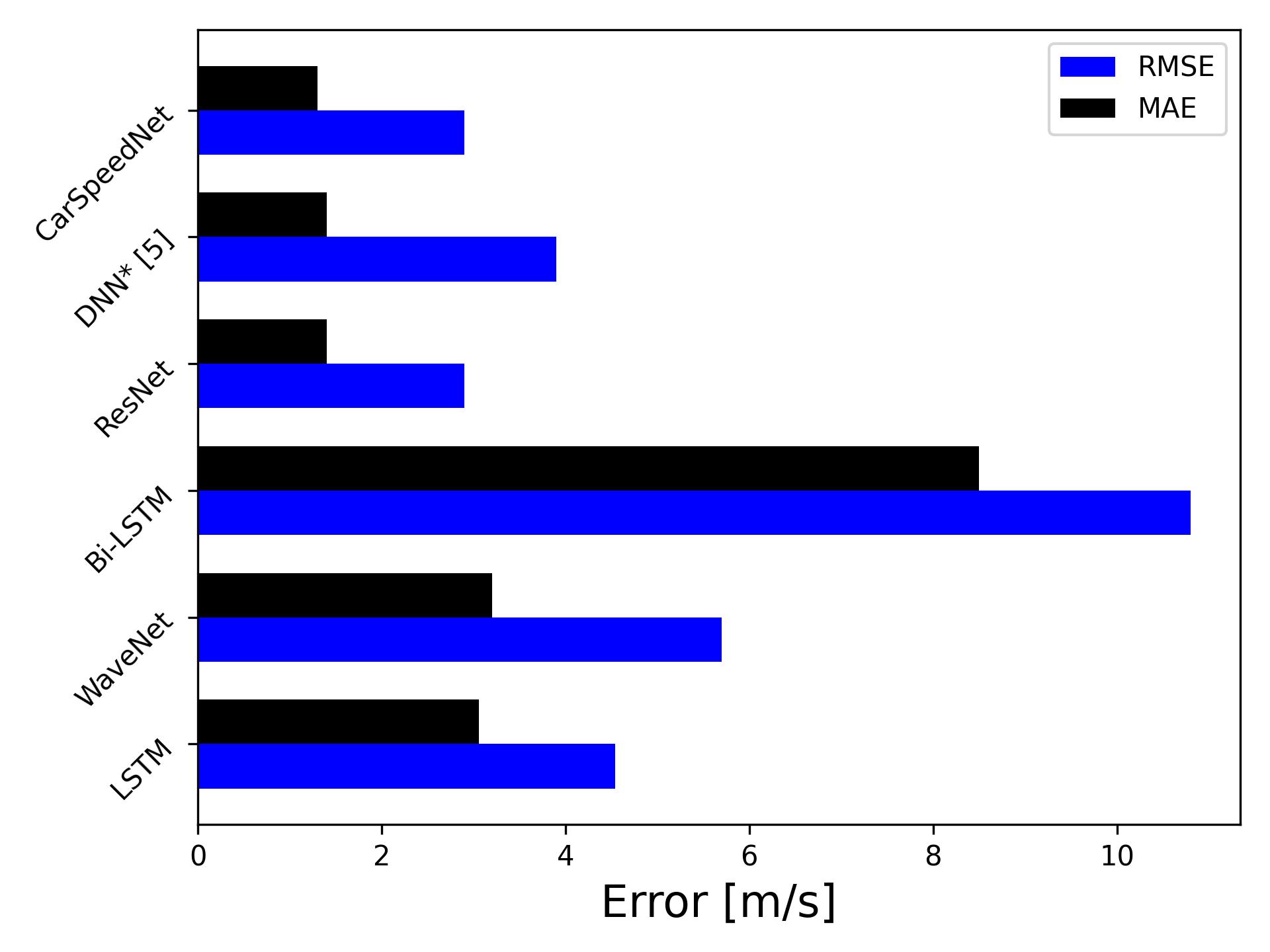
Figure 4: Models’ performance evaluation using the RMSE and MAE metrics. DNN* is the architecture from previous work [2], trained with accelerometer data only.

III-C The effect of input size on CarSpeedNet

In this investigation, we delve into the impact of varying input sizes on the performance of CarSpeedNet. The study examines the consequences of altering the temporal window size of the input data, which is composed of tri-axial signal measurements (x, y, and z directions) captured at a rate of 20 [m/s].

An important aspect of this exploration is the relationship between the input window size and the resultant latency in speed estimation. For instance, an input batch corresponding to a 4-second window necessitates a 4-second wait to accumulate data before it can be processed by the network. This implies an inherent delay in speed calculation equivalent to the window size. Consequently, with a 4-second window, the network’s speed estimation reflects an average over the past 4 [s]. This study methodically varied the input window size from 0.25 [s] (5 measurements) to 4 [s] (80 measurements), with each variant necessitating a distinct model training and testing cycle, thereby yielding separate models for each window size.

The findings of this study are systematically tabulated in Table I, which presents a comparative analysis across different window sizes, highlighting the RMSE, MAE, and latency associated with each window size. The table indicates a clear trend: as the window size increases, there is a noticeable improvement in accuracy, as evidenced by lower RMSE and MAE values. For instance, the largest window size of 80 measurements (4 [s]) achieved the lowest RMSE of 1.8 [m/s] and MAE of 0.72 [m/s], underscoring the enhanced accuracy at larger window sizes. However, this improvement in accuracy comes at the cost of increased latency, an important factor to consider in real-time applications.

Additionally, the temporal performance of CarSpeedNet, encompassing the comparison between the estimated speeds by the model and the actual speeds (ground truth), was plotted over time for each input window size. These plots, presented in Figures 6-11, offer a visual representation of the model’s performance across different window sizes.

It is observed that CarSpeedNet demonstrates a high degree of accuracy in estimating speeds during slow-moving conditions. This precision at lower velocities is a testament to the model’s sensitivity and effectiveness in capturing subtle variations in the accelerometer data, which are prevalent at reduced speeds.

Significantly, the model’s proficiency is further highlighted in its capability to accurately detect stationary conditions. In instances where the car is at a complete halt, CarSpeedNet’s estimated speed closely aligns with zero. This ability to discern and accurately indicate a state of rest is a critical feature for any speed estimation model, as it ensures reliable performance across the entire spectrum of vehicular motion, from high-speed travel to complete stops.

TABLE I: Input size influance

Window size	RMSE [m/s]	MAE [m/s]	Latency [ms]
5 / 0.25[s]	4.9	2.5	96.5
10 / 0.5[s]	4.2	2.1	177
20 / 1[s]	2.9	1.3	100
40 / 2[s]	2.3	1	94
60 / 3[s]	2.2	0.88	102.4
80 / 4[s]	1.8	0.72	104.8

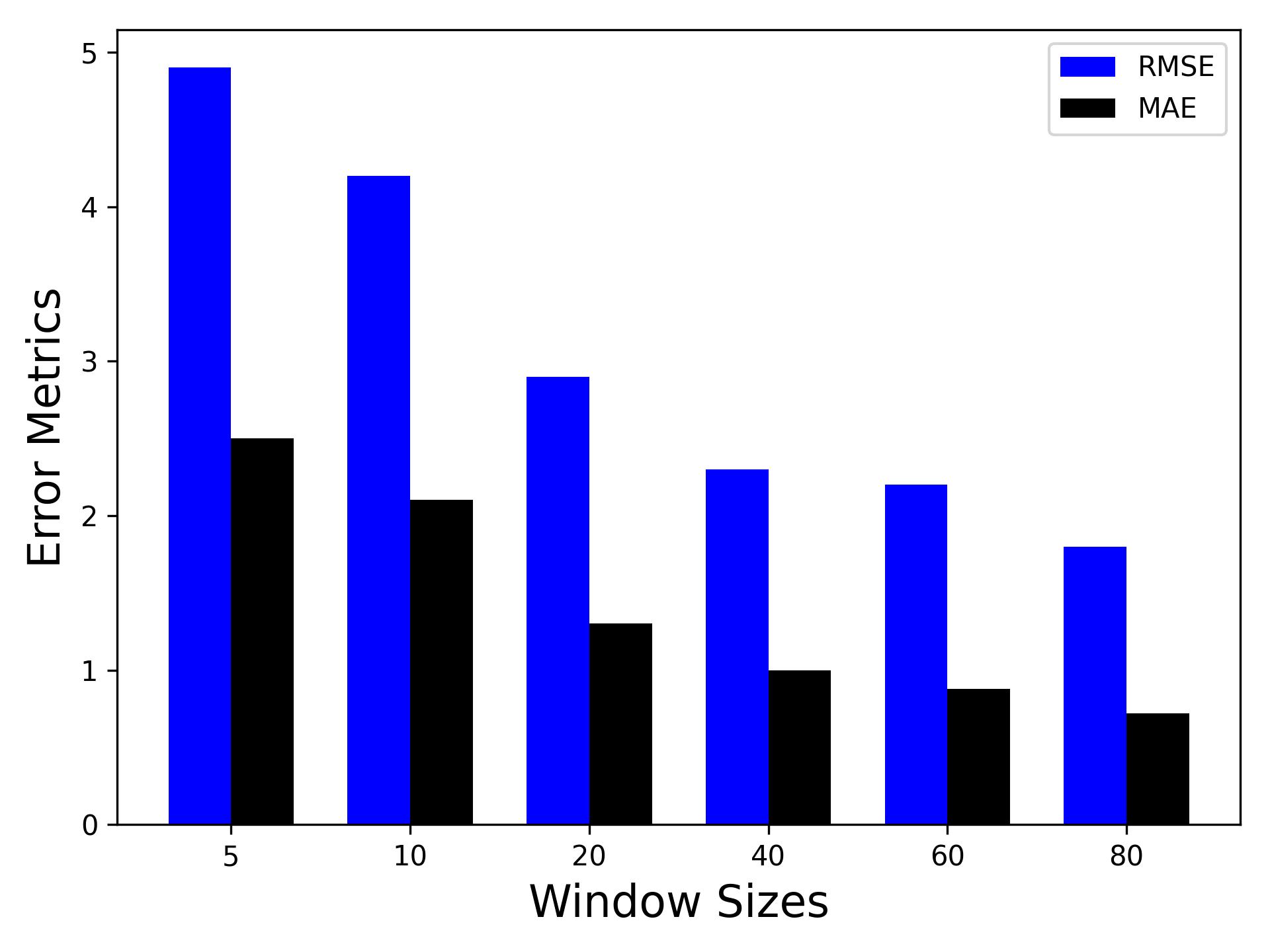
Figure 5: CarSpeedNet performance as a function of the input size

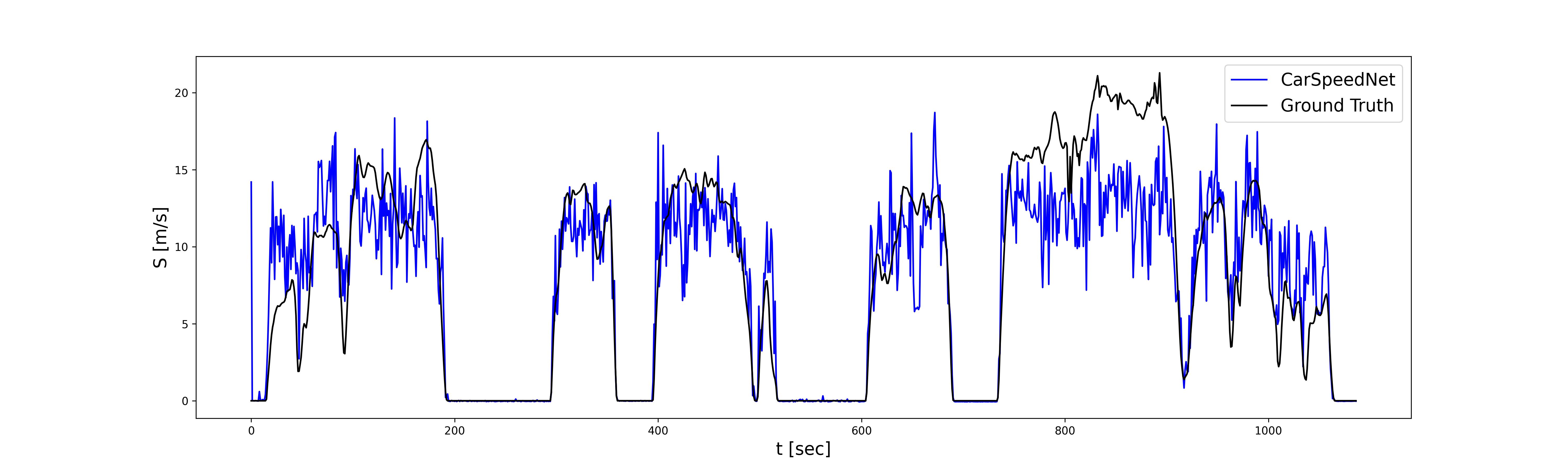
Figure 6: CarSpeedNet vs. GT speed comparison, w=5

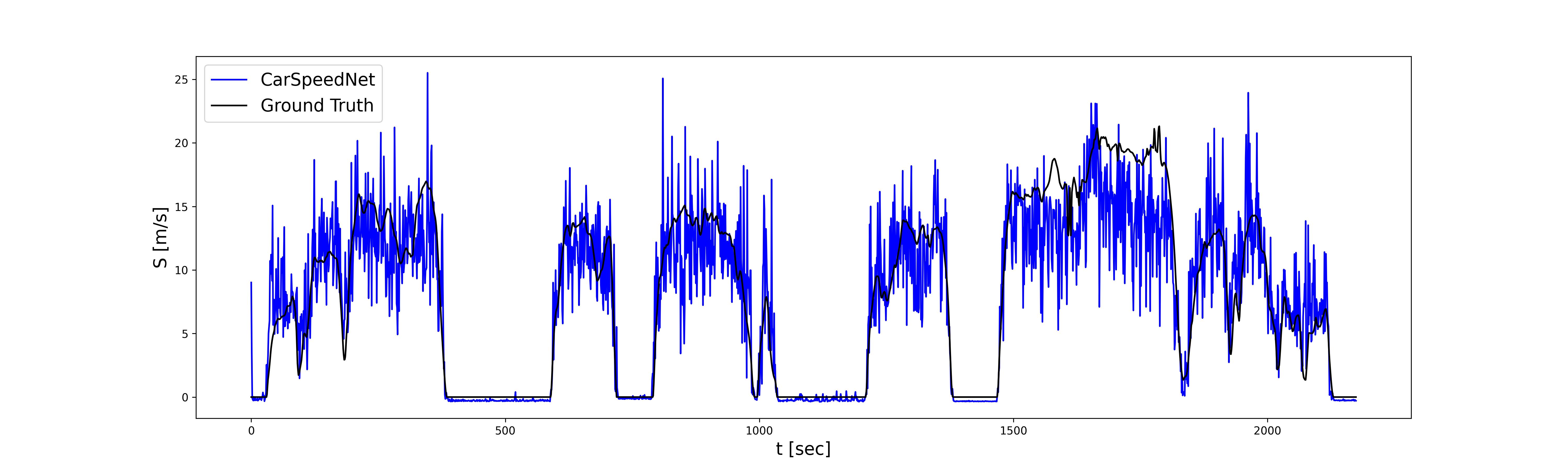
Figure 7: CarSpeedNet vs. GT speed comparison, w=10

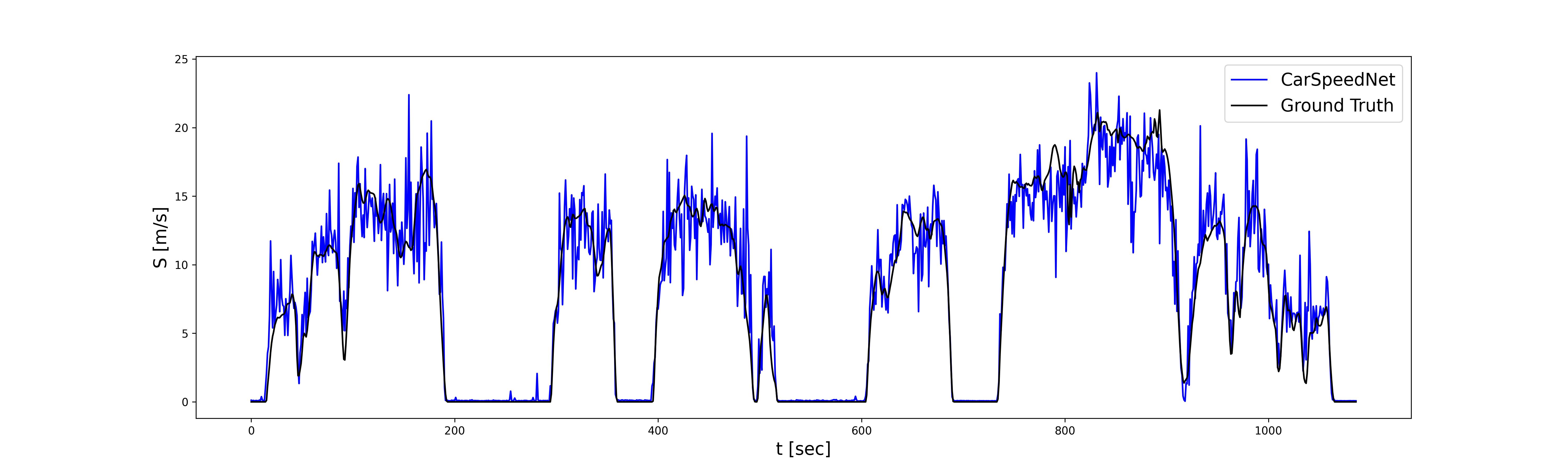
Figure 8: CarSpeedNet vs. GT speed comparison, w=20

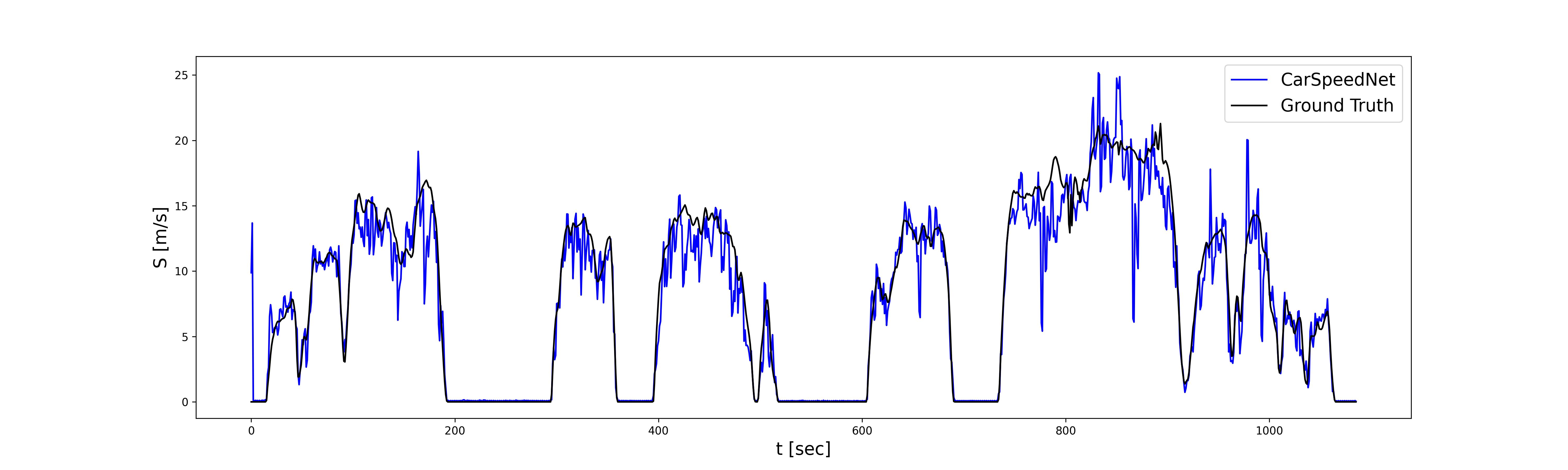
Figure 9: CarSpeedNet vs. GT speed comparison, w=40

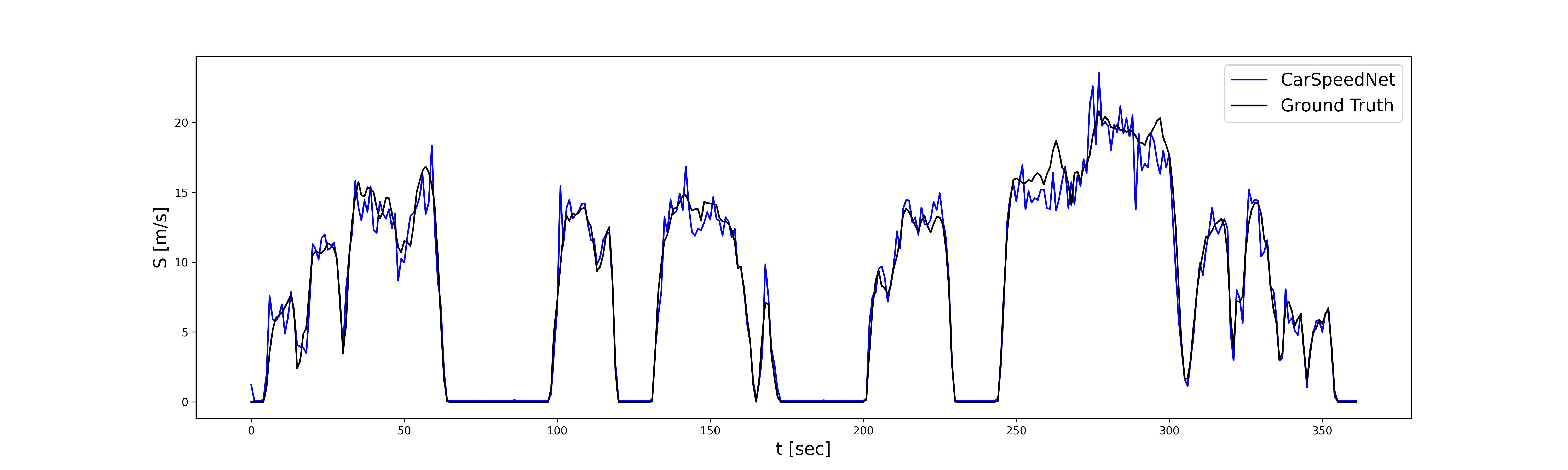
Figure 10: CarSpeedNet vs. GT speed comparison, w=60

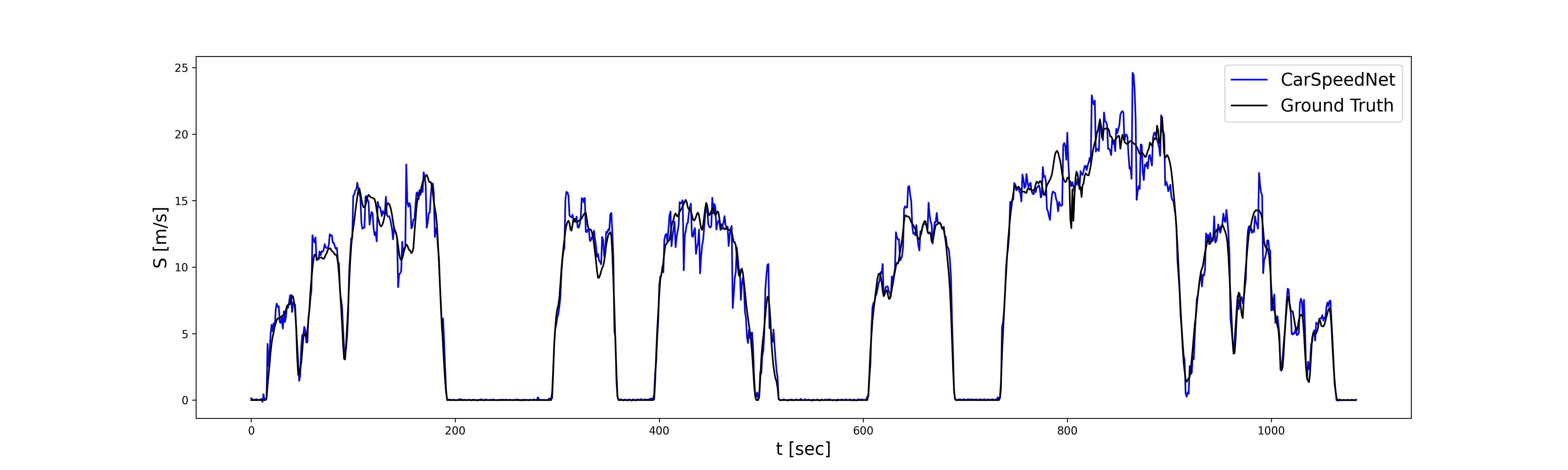
Figure 11: CarSpeedNet vs. GT speed comparison, w=80

III-D Real-Time Applications

The suggested model also offers significant real-time utility. This versatility is particularly valuable in scenarios where multiple cars need to report their speeds to a central cloud system. One of the model’s key advantages is its capability to provide speed information in near real-time. It operates seamlessly with smartphone accelerometer data, eliminating the need for a connection to the car’s Controller Area Network (CAN BUS). This inherent adaptability makes it highly accessible across a wide spectrum of cars without requiring car-specific integration or hardware modifications.

• Transportation management: Consider a bus transportation system as an example. The model can provide real-time updates on bus speed, allowing for proactive monitoring of driver adherence to speed limits. This not only enhances passenger safety but also assists in optimizing fuel efficiency and reducing car wear and tear.

• Individual driver control: For individual drivers, this model offers the ability to share real-time speed notifications with supervisors or parents. This feature proves especially valuable for monitoring young or inexperienced drivers, ensuring their compliance with safe driving practices.

• Insurance industry: By accessing real-time speed data, insurance providers can offer usage-based insurance policies, adjusting premiums based on an individual’s driving behavior. This not only rewards safe drivers with lower rates but also encourages responsible driving habits.

• Traffic management: In a broader traffic management context, our model can contribute to detecting traffic congestion and the development of traffic jams. Traditional GPS-based systems may not accurately capture motion properties for detecting accelerations and decelerations. Our model, through continuous monitoring of accelerometer data, can provide valuable real-time insights into the actual state of the car, aiding in more effective traffic flow management.

• Adaptable time windows: One of the distinctive features of our model is its adaptability regarding time windows. While there is a 4-second delay inherent in the general prediction system, this may be irrelevant in certain situations. For instance, if the objective is to detect instances of high-speed driving for extended durations, this delay may not be a significant concern. However, if the intention is to implement a notification system that enforces speed limits within a shorter timeframe, a 0.5 [s] window, for example, can be employed.

IV Conclusions

In this study we presented an advancement in the field of car speed estimation by introducing CarSpeedNet, a deep neural network model utilizing smartphone accelerometer data. The model demonstrates high precision in speed estimation, addressing the limitations of traditional car-based systems and providing a universally accessible solution. The model demonstrates a precision of less than 0.72[m/s] during extended driving tests.

Key findings include the optimal window size for data input, where larger window sizes led to improved accuracy but at the cost of increased latency, crucial for real-time applications. The comprehensive approach to data collection and training ensures the model’s practical effectiveness in real-world scenarios. This research paves the way for further exploration in leveraging smartphone technology for traffic management and safety, offering an innovative approach to intelligent transportation systems.

Barak Or (Member, IEEE) received a B.Sc. degree in aerospace engineering (2016), a B.A. degree (cum laude) in economics and management (2016), and an M.Sc. degree in aerospace engineering (2018) from the Technion–Israel Institute of Technology. He graduated with a Ph.D. degree from the University of Haifa, Haifa (2022). His research interests include navigation, deep learning, sensor fusion, and estimation theory.

References

- [1] Z. Armah, I. Wiafe, F. Koranteng, and E. Owusu, “Speed monitoring and controlling systems for road vehicle safety: a systematic review.” Advances in Transportation Studies, vol. 56, 2022.
- [2] M. Freydin and B. Or, “Learning car speed using inertial sensors for dead reckoning navigation,” IEEE Sensors Letters, vol. 6, no. 9, pp. 1–4, 2022.
- [3] H. Dong, M. Wen, and Z. Yang, “Vehicle speed estimation based on 3d convnets and non-local blocks,” Future Internet, vol. 11, no. 6, p. 123, 2019.
- [4] B. Or and I. Klein, “Learning vehicle trajectory uncertainty,” Engineering Applications of Artificial Intelligence, vol. 122, p. 106101, 2023.
- [5] J. Farrell, Aided navigation: GPS with high rate sensors. McGraw-Hill, Inc., 2008, pp: 393-395.
- [6] W. Kerber, “Data governance in connected cars: the problem of access to in-vehicle data,” J. Intell. Prop. Info. Tech. & Elec. Com. L., vol. 9, p. 310, 2018.
- [7] C. Campolo, A. Iera, A. Molinaro, S. Y. Paratore, and G. Ruggeri, “Smartcar: An integrated smartphone-based platform to support traffic management applications,” in 2012 first international workshop on vehicular traffic management for smart cities (VTM). IEEE, 2012, pp. 1–6.
- [8] V. Astarita, D. C. Festa, and V. P. Giofrè, “Mobile systems applied to traffic management and safety: a state of the art,” Procedia computer science, vol. 134, pp. 407–414, 2018.
- [9] A. Ali, N. Ayub, M. Shiraz, N. Ullah, A. Gani, and M. A. Qureshi, “Traffic efficiency models for urban traffic management using mobile crowd sensing: A survey,” Sustainability, vol. 13, no. 23, p. 13068, 2021.
- [10] Y. Yao, X. Zhao, C. Liu, J. Rong, Y. Zhang, Z. Dong, and Y. Su, “Vehicle fuel consumption prediction method based on driving behavior data collected from smartphones,” Journal of Advanced Transportation, vol. 2020, pp. 1–11, 2020.
- [11] E. Mantouka, E. Barmpounakis, E. Vlahogianni, and J. Golias, “Smartphone sensing for understanding driving behavior: Current practice and challenges,” International journal of transportation science and technology, vol. 10, no. 3, pp. 266–282, 2021.
- [12] Y. Li, R. Chen, X. Niu, Y. Zhuang, Z. Gao, X. Hu, and N. El-Sheimy, “Inertial sensing meets machine learning: Opportunity or challenge?” IEEE Transactions on Intelligent Transportation Systems, 2021.
- [13] Y. LeCun, Y. Bengio, and G. Hinton, “Deep learning,” nature, vol. 521, no. 7553, pp. 436–444, 2015.
- [14] J. Zhang, W. Xiao, B. Coifman, and J. P. Mills, “Vehicle tracking and speed estimation from roadside lidar,” IEEE Journal of Selected Topics in Applied Earth Observations and Remote Sensing, vol. 13, pp. 5597–5608, 2020.
- [15] D. Fernandez Llorca, A. Hernandez Martinez, and I. Garcia Daza, “Vision-based vehicle speed estimation: A survey,” IET Intelligent Transport Systems, vol. 15, no. 8, pp. 987–1005, 2021.
- [16] J. Yu, M. E. Stettler, P. Angeloudis, S. Hu, and X. M. Chen, “Urban network-wide traffic speed estimation with massive ride-sourcing gps traces,” Transportation Research Part C: Emerging Technologies, vol. 112, pp. 136–152, 2020.
- [17] Q. Wang, Y. Gu, J. Liu, and S. Kamijo, “Deepspeedometer: Vehicle speed estimation from accelerometer and gyroscope using lstm model,” in 2017 IEEE 20th International Conference on Intelligent Transportation Systems (ITSC). IEEE, 2017, pp. 1–6.
- [18] I. Ustun and M. Cetin, “Speed estimation using smartphone accelerometer data,” Transportation research record, vol. 2673, no. 3, pp. 65–73, 2019.
- [19] N. E. A. Abdelgawad, A. El Mahdy, W. Gomaa, and A. Shoukry, “Estimating vehicle speed on highway roads from smartphone sensors using deep learning models,” in 2019 IEEE 31st International Conference on Tools with Artificial Intelligence (ICTAI). IEEE, 2019, pp. 979–986.
- [20] I. Sharp, K. Yu, and Y. J. Guo, “Gdop analysis for positioning system design,” IEEE Transactions on Vehicular Technology, vol. 58, no. 7, pp. 3371–3382, 2009.
- [21] S. Hochreiter and J. Schmidhuber, “Long short-term memory,” Neural computation, vol. 9, no. 8, pp. 1735–1780, 1997.
- [22] P. Zhou, W. Shi, J. Tian, Z. Qi, B. Li, H. Hao, and B. Xu, “Attention-based bidirectional long short-term memory networks for relation classification,” in Proceedings of the 54th annual meeting of the association for computational linguistics (volume 2: Short papers), 2016, pp. 207–212.
- [23] A. v. d. Oord, S. Dieleman, H. Zen, K. Simonyan, O. Vinyals, A. Graves, N. Kalchbrenner, A. Senior, and K. Kavukcuoglu, “Wavenet: A generative model for raw audio,” arXiv preprint arXiv:1609.03499, 2016.
- [24] K. He, X. Zhang, S. Ren, and J. Sun, “Deep residual learning for image recognition,” in Proceedings of the IEEE conference on computer vision and pattern recognition, 2016, pp. 770–778.
- [25] D. P. Kingma and J. Ba, “Adam: A method for stochastic optimization,” arXiv preprint arXiv:1412.6980, 2014.