Spectral analysis of periodic $b$-KP equation under transverse perturbation

Abstract.

The $b$-family-Kadomtsev-Petviashvili equation ($b$-KP) is a two dimensional generalization of the $b$-family equation. In this paper, we study the spectral stability of the one-dimensional small-amplitude periodic traveling waves with respect to two-dimensional perturbations which are either co-periodic in the direction of propagation, or nonperiodic (localized or bounded). We perform a detailed spectral analysis of the linearized problem associated to the above mentioned perturbations, and derive various stability and instability criteria which depends in a delicate way on the parameter value of $b$, the transverse dispersion parameter $\sigma$, and the wave number $k$ of the longitudinal waves.

Keywords: $b$-Kadomtsev-Petviashvili equation, Camassa-Holm-Kadomtsev-Petviashvili equation, periodic traveling waves, transverse spectral stability

AMS Subject Classification (2010): 35B35, 35C07, 37K45.

1. Introduction

In the study of wave phenomena, particularly in dispersive and nonlinear media, the emergence of periodic wave trains stands out as a captivating outcome arising from the intricate interplay between dispersion and nonlinearity. These wave patterns manifest across diverse physical domains, encompassing phenomena such as water waves, nonlinear optics, acoustics, and plasma. Given their pervasive presence in nature, the investigation of periodic wave trains continues to attract considerable interest from scientists and researchers.

One important question is the stability of the periodic waves. Stability properties govern the long-term behavior of the wave patterns and play a crucial role in understanding the robustness and predictability of the phenomena they represent. While many physical systems support unidirectional wave propagation, which can be modeled by equations in a single spatial dimension, it is crucial to acknowledge that in a multi-dimensional context, transverse effects become integral. Consequently, the stability analysis of one-dimensional traveling waves, particularly concerning perturbations propagating along the transverse direction of the primary axis – referred to as transverse stability – becomes a naturally compelling avenue of interest. This exploration extends beyond the traditional analysis of responses to perturbations along the main propagation axis, providing a more comprehensive understanding of the intricate dynamics governing wave stability in multi-dimensional settings.

Such a problem was first studied by Kadomtsev and Petviashvili [23], who derived a two-dimensional generalization of the celebrated KdV equation, the so-called Kadomtsev-Petviashvili (KP) equation. They found that the KdV localized solitons in the KP flow are stable to transverse perturbations in the case of negative dispersion (KP-II), while unstable by long wavelength transverse perturbations for the positive dispersion model (KP-I). Later development of the theory for solitary waves includes the use of integrability [33], explicit spectral analysis [2], perturbation analysis [24], general Hamiltonian PDE techniques [31, 30], Miura transformation [28], the combination of algebraic properties, weighted function spaces, and refined PDE tools [26, 27], among others.

When periodic waves are considered, to the authors’ knowledge, most of the study of transverse stability pertains to spectral analysis; see for e.g., [32, 21, 16, 17, 3] for the KP and generalized KP equations, [13, 1] for the nonlinear Schrödinger (NLS) equation, and [5, 20, 29] for the Zakharov-Kuznetsov (ZK) equation.

The goal of this paper is to extend the transverse stability analysis to periodic waves arising from models exhibiting strong non-local and nonlinear features. Specifically, we choose the one-dimensional $b$-family equation [14]

$$\left(1-\partial_{x}^{2}\right)u_{t}+(b+1)uu_{x}+\kappa u_{x}-bu_{x}u_{xx}-uu_{xxx}=0,\quad u=u(t,x),\ \ b\in{\mathbb{R}},\kappa>0,$$ (1.1)

and consider its two-dimensional generalization

$$\left[\left(1-\partial_{x}^{2}\right)u_{t}+(b+1)uu_{x}+\kappa u_{x}-bu_{x}u_{xx}-uu_{xxx}\right]_{x}+\sigma u_{yy}=0,\quad\sigma=\pm 1,$$ (1.2)

where the profile $u=u(t,x,y)$. We refer to (1.2) as the $b$-KP equation due to the resemblance of transverse term $\sigma u_{yy}$ to that of the classical KP equation; and in a similar way, the $b$-KP equation with $\sigma=-1$ is called the $b$-KP-I equation, whereas the one with $\sigma=1$ is called the $b$-KP-II equation. The physical relevance of the $b$-KP equation (1.2) has been recently discovered in the context of shallow water waves [22, 12] and nonlinear elasticity [6], for the case $b=2$. The corresponding equation is also referred to as the CH-KP equation as it generalizes the well-known Camassa–Holm equation [4].

While the (longitudinal) stability of solitary and periodic waves of the $b$-family equation (1.1) has been studied quite extensively, the understanding of the local dynamics of these waves under the $b$-KP flow is much less developed. The only results that the authors are aware of regard the line solitary waves of the CH-KP equation: the nonlinear transverse instability of the solitary waves to the CH-KP-I equation is established in [7], and linear stability of small-amplitude solitary waves is confirmed for CH-KP-II very recently [9].

In this paper, we will investigate the transverse spectral stability/instability of small periodic traveling waves of the $b$-family equation (1.1) with respect to perturbations in the $b$-KP flow. Compared with the study of solitary waves, the stability of periodic waves is usually more delicate. The periodic waves in general exhibit a richer structural complexity, characterized by dependencies on three parameters – namely, the period, wave speed, and integration constant. Such higher degree of freedom often introduces additional technical difficulties not encountered in the analysis of solitary waves. Moreover, a more broader class of perturbations can be considered for periodic waves, encompassing co-periodic, multiple-periodic, localized perturbations, among others. Our motivation for specifically studying the small-amplitude period waves is inspired by the work of Haragus [16], where perturbation arguments have been successfully employed to discern the spectra of the linear operator. In contrast to the stability analysis of large waves, where instability criteria can usually be derived (in the particular case of integrable systems, explicit computation can be performed, but (1.2) is in general non-integrable), our choice to work with small-amplitude waves is motivated by the potential for obtaining more explicit information on the spectra, and for allowing for a broader range of perturbation types.

1.1. Main results

Although the basic idea of the approach stems from the work of Haragus [16], the quasilinear structure of the equation (1.2) makes the spectral computation a lot more involved. For the case of $b$-KP-I flow $\sigma=-1$ with co-periodic perturbations in the direction of propagation (see Section 3 for a precise definition of the class of perturbations and the corresponding notion of spectral stability), the linearized problem does not assume a natural Hamiltonian structure, and hence the standard index counting method cannot be applied directly. On the other hand, the linearized operator at the trivial solution does admit a decomposition into a composition of a skew-adjoint operator with a self-adjoint operator, and thus the counting result can be used to provide direct insights for the spectrum of this operator. Such information can then be transferred to the linearized operators at small-amplitude waves. Through a careful perturbation argument and explicit computation on the expansion of the spectra, we confirm the emergence of long-wave transverse instability for a range of $b$, which includes the examples of CH-KP ($b=2$) and Degasperis–Procesi(DP)-KP ($b=3$). More interestingly, depending on the wave number $k$ of the line periodic waves, there also exists a large region of values of $b$ where the line periodic waves are transversally spectrally stable.

In contrast to the $b$-KP-I equation, the spectral analysis for the $b$-KP-II equation ($\sigma=1$) presents a more intricate challenge, reminiscent of the complexities found in the classical KP-II equation. The computation of the spectrum becomes substantially more complicated due to the nature of the dispersion relation, which is more likely to host unstable modes. Notably, in the limit of zero transverse wavelength, the dispersion relation may harbor an infinite number of potentially unstable eigenvalues. Tracking the locations of these eigenvalues further adds to the complexity, requiring the computation of the Taylor expansion of the corresponding eigen-matrix to an arbitrarily high order. The difficulties involved in these computations make it exceptionally challenging to achieve a comprehensive spectral analysis. What we are able to conclude in this case is a characterization of the spectra under long wavelength transverse perturbations. While a complete spectral analysis remains elusive, our findings align well with the spectral stability observed in the context of CH-KP-II solitary waves [9].

Theorem 1.1 (Informal statement of transverse stability for periodic perturbation).

Let $b\neq-1$. Consider a $2\pi/k$-periodic traveling wave solution of (1.1) constructed in Lemma 2.1.

1. For $\sigma=-1$ ($b$-KP-I) and the amplitude of the wave is sufficiently small, such a wave is transversely spectrally unstable with respect to co-periodic perturbations in the $x$-direction and periodic in the $y$-direction, when the parameters $(b,k^{2})$ lie outside the shaded region showed in Figure 1. This wave is transversely spectrally stable otherwise, provided that the wave is spectrally stable with respect to longitudinal perturbations.

2. For $\sigma=1$ ($b$-KP-II) and the amplitude of the wave is sufficiently small, such a wave is transversely spectrally unstable with respect to co-periodic perturbations in the $x$-direction and periodic in the $y$-direction, when the parameters $(b,k^{2})$ lie inside the shaded region showed in Figure 1. Otherwise this wave is transversely spectrally stable under long-wave transverse perturbation, provided that the wave is spectrally stable with respect to longitudinal perturbations.

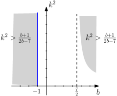
Figure 1. A schematic plot of the stability region for the periodic perturbation of the $b$-KP flow. The two shaded regions correspond to $\{(b,k^{2}):b<-1,k^{2}>\frac{b+1}{2b-7}\}$ and $\{(b,k^{2}):b>\frac{7}{2},k^{2}>\frac{b+1}{2b-7}\}$.

For non-periodic perturbations in the direction of propagation, the linearized operator has bands of continuous spectra. Since the coefficients of the operator are periodic, we will use the classical Floquet-Bloch theory to replace the study of the invertibility of the original linearized operator by the invertibility of a family of Bloch operators in parameterized by the Floquet exponent (see Lemma 5.1). Through a detailed calculation of the spectrum of the linearized operator at the trivial solution (zero-amplitude solution), a perturbation argument is performed, which allows one to derive instability criterion for the $b$-KP-I case. We would like to point out that, a complete understanding of the Floquet analysis for the linearized operator is exceedingly difficult due to the appearance of the terms corresponding to the smoothing operator in the dispersion relation. Instead, when focused on the regime where the transverse perturbations are of finite wavelength, we manage to track the location where there is exactly one collision between a pair of eigenvalues of the linearized operator at the trivial solution from the imaginary axis, which results in the bifurcation of the unstable eigenvalues of the full linearized problem. The exact statement of the results is given in Theorem 5.1. For long-wavelength transverse perturbations, an additional condition on the longitudinal wavelength is needed in order to eliminate the eigenvalue collisions. The detailed discussion is provided in Section 5.5.

The remainder of this paper is organized as follows. In Section 2, we use the Lyapunov-Schmidt reduction to construct the family of the one-dimensional small-amplitude periodic traveling waves of the $b$-KP equation and provide a parameterization of these waves. In Section 3, we formulate the spectral problem for the $b$-KP equation and introduce the definition of spectral stability in various function space settings. In Sections 4 and 5, we discuss the spectra of the resulting linear operators, and investigate the transverse spectral stability/instability of the small periodic waves of the $b$-KP-I and $b$-KP-II equation for periodic and non-periodic perturbations.

1.2. Notations

Throughout this paper, we will use the following notations. The space $L^{2}(\mathbb{R})$ denotes the set of real or complex-valued, Lebesgue measurable functions over $\mathbb{R}$ such that

$$\|f\|_{L^{2}(\mathbb{R})}=\left(\int_{\mathbb{R}}|f(x)|^{2}\mathrm{~{}d}x\right)^{1/2}<+\infty,$$

and $L^{2}(\mathbb{T})$ denotes the space of $2\pi$-periodic, measurable, real or complex-valued functions over $\mathbb{R}$ such that

$$\|f\|_{L^{2}(\mathbb{T})}=\left(\frac{1}{2\pi}\int_{0}^{2\pi}|f(x)|^{2}\mathrm{~{}d}x\right)^{1/2}<+\infty.$$

The space $C_{\textup{bdd}}(\mathbb{R})$ contains all bounded continuous functions on $\mathbb{R}$, normed with

$$\|f\|=\sup_{x\in\mathbb{R}}|f(x)|.$$

For $s\in\mathbb{R}$, let $H^{s}(\mathbb{R})$ consist of tempered distributions such that

$$\|f\|_{H^{s}(\mathbb{R})}=\left(\int_{\mathbb{R}}\left(1+|t|^{2}\right)^{s}|\widehat{f}(t)|^{2}\mathrm{~{}d}t\right)^{1/2}<+\infty,$$

where $\widehat{f}$ is the Fourier transform of $f$, and

$$H^{s}(\mathbb{T})=\left\{f\in H^{s}(\mathbb{R}):f\text{ is }2\pi\text{-periodic}\right\}.$$

We define the $L^{2}(\mathbb{T})$-inner product as

$$\langle f,g\rangle=\frac{1}{2\pi}\int_{0}^{2\pi}f(z)\bar{g}(z)\mathrm{d}z=\sum_{n\in\mathbb{Z}}\widehat{f}_{n}\overline{\widehat{g}}_{n},$$ (1.3)

where $\widehat{f}_{n}$ are Fourier coefficients of the function $f$ defined by

$$\widehat{f}_{n}=\frac{1}{2\pi}\int_{0}^{2\pi}f(z)\mathrm{e}^{inz}dz.$$

We denote $\Re(\lambda)$ the real part of $\lambda\in\mathbb{C}$.

2. Existence of small periodic traveling waves

One-dimensional traveling waves of the $b$-KP equation (1.2) are solutions of the form

$$u(x,y,t)=u(x-ct),$$

where $c>0$ is the speed of propagation, and $u$ satisfies the ODE

$$\left[-c\left(u^{\prime}-u^{\prime\prime\prime}\right)+(b+1)uu^{\prime}+\kappa u^{\prime}-bu^{\prime}u^{\prime\prime}-uu^{\prime\prime\prime}\right]^{\prime}=0.$$

Integrating this equation twice, and writing $x$ instead of $x-ct$, we obtain the second order ODE

$$(\kappa-c)u+cu^{\prime\prime}+\frac{b+1}{2}u^{2}-uu^{\prime\prime}-\frac{b-1}{2}\left(u^{\prime}\right)^{2}=Ax-m(c-\kappa)^{2},$$

in which $A$ and $m$ are arbitrary integration constants. Considering periodic solutions, we set $A=0$ and the equation reduces to

$$(\kappa-c)u+cu^{\prime\prime}+\frac{b+1}{2}u^{2}-uu^{\prime\prime}-\frac{b-1}{2}\left(u^{\prime}\right)^{2}=-m(c-\kappa)^{2}.$$ (2.1)

Since this equation does not possess scaling and Galilean invariance, we may not simply assume that $c=1,m=0$.

Let $u$ be a $2\pi/k$-periodic function of its argument, for some $k>0$. Then, $w(z):=u(x)$ with $z=kx$, is a $2\pi$-periodic function in $z$, satisfying

$$(\kappa-c)w+ck^{2}w_{zz}+\frac{b+1}{2}w^{2}-k^{2}ww_{zz}-\frac{b-1}{2}k^{2}w_{z}^{2}=-m(c-\kappa)^{2}.$$ (2.2)

Let $F:H^{2}_{2\pi}(\mathbb{T})\times\mathbb{R}_{+}\times\mathbb{R}\times\mathbb{R}\rightarrow L^{2}(\mathbb{T})$ be defined as

$$F(w;k,c,m)=(\kappa-c)w+ck^{2}w_{zz}+\frac{b+1}{2}w^{2}-k^{2}ww_{zz}-\frac{b-1}{2}k^{2}w_{z}^{2}+m(c-\kappa)^{2}.$$ (2.3)

We seek a solution $w\in H^{2}(\mathbb{T})$ of

$$F(w;k,c,m)=0.$$ (2.4)

Noting that (2.3) remains invariant under $z\mapsto z+z_{0}$, $z\mapsto-z$ for any $z_{0}\in\mathbb{R}$, we may assume that $w$ is even. Clearly $F$ is analytic on its arguments.

It is easy to see that a constant solution $w_{0}$ of equation (2.4) satisfies

$$\frac{b+1}{2}w_{0}^{2}+(\kappa-c)w_{0}+m(c-\kappa)^{2}=0.$$ (2.5)

For $c\in\mathbb{R}$ and $\kappa>0$, when $b=-1$ we have

$$w_{0}=w_{0}(m)=\left\{\begin{aligned} &m(c-\kappa),\ &\text{ when }c\neq\kappa,\\ &\text{any constant,}\ &\text{ when }c=\kappa.\end{aligned}\right.$$

When $b\neq-1$, and $2m(b+1)<1$, (2.5) is a genuine quadratic equation, and we find

$$w_{0}(m)=\frac{c-\kappa\pm|c-\kappa|\sqrt{1-2m(b+1)}}{b+1}.$$

It follows from the implicit function theorem that if non-constant solutions of (2.4) (and hence (2.2)) bifurcate from $w=w_{0}$ for some $c=c_{0}$ then necessarily,

$$L_{0}:=\partial_{w}F\left(w_{0};c_{0},k,m\right):H^{2}(\mathbb{T})\rightarrow L^{2}(\mathbb{T})$$

is not an isomorphism, where

$$L_{0}=k^{2}\left(c_{0}-(b-1)w_{0}\right)\partial_{z}^{2}+\left(\kappa-c_{0}\right)+(b+1)w_{0}.$$

Further calculation reveals that $L_{0}e^{inz}=0,n\in\mathbb{Z}$, if and only if

$$c_{0}=\frac{\kappa}{1+k^{2}n^{2}}+w_{0}\frac{(b+1)+k^{2}n^{2}(b-1)}{1+k^{2}n^{2}},$$ (2.6)

which, when plugging in the form of $w_{0}$, would lead to a solution

$$c_{0}=c_{0}(k,m),$$

at least for $m$ sufficiently small.

Without loss of generality, we restrict our attention to $|n|=1$, to further simplify the analysis, we take the constant $m=0$, and consider the constant solution $w_{0}=0$. This way (2.6) leads to

$$c_{0}=c_{0}(k)=\frac{\kappa}{1+k^{2}}.$$

In this case it is straightforward to verify that the kernel of $L_{0}$ : $H^{2}(\mathbb{T})\rightarrow L^{2}(\mathbb{T})$ is two-dimensional and spanned by $e^{\pm iz}$. Moreover, the co-kernel of $L_{0}$ is two-dimensional. Therefore, $L_{0}$ is a Fredholm operator of index zero. One may then follow an idea similar to that of [18, 19] to employ a Lyapunov-Schmidt reduction and construct a one parameter family of non-constant, even and smooth solutions of (2.1) near $w=w_{0}=0$ and $c=c_{0}(k)$. The small-amplitude expansion of these solutions is given as follows and the details are provided in Appendix A.

Lemma 2.1.

For each $\kappa,k>0$, and $m=0$, there exists a family of small amplitude $2\pi/k$-periodic traveling waves of (1.2)

$$w(k,a):=u\left(k\left(x-c(k,a)t\right)\right)$$ (2.7)

for $|a|$ sufficiently small; $w$ and $c$ depend analytically on $k$ and $a$, $w$ is smooth, even and $2\pi$-periodic in $z$, and $c$ is even in $a$. Furthermore, as $a\to 0$,

$$w(k,a)= \ a\cos z+a^{2}\left(A_{0}+A_{2}\cos 2z\right)+a^{3}A_{3}\cos 3z+O\left(a^{4}\right),$$ (2.8)

$$c(k,a)= \ c_{0}+a^{2}c_{2}+O\left(a^{4}\right),$$ (2.9)

with

$$\begin{array}[]{ll}\displaystyle A_{0}=\frac{\left(1+k^{2}\right)}{4\kappa k^{2}}\left({(b-3)}k^{2}-{(b+1)}\right),\quad A_{2}=\frac{{(b+1)}\left(1+k^{2}\right)^{2}}{12\kappa k^{2}},\\ \\ \displaystyle A_{3}=\frac{{(b+1)}\left(k^{2}+1\right)^{3}}{192\kappa^{2}k^{4}}\left({{(2b+3)}k^{2}+(b+1)}\right),\\ \\ \displaystyle c_{0}=\frac{\kappa}{1+k^{2}},\quad c_{2}=\frac{1}{\kappa}\left({\frac{-2b^{2}+11b-11}{24}k^{2}+\frac{5b^{2}-11b-16}{24}-\frac{5(b+1)^{2}}{24k^{2}}}\right).\end{array}$$ (2.10)

3. Formulation of the spectral problem

Linearizing the $b$-KP equation (1.2) about its one-dimensional periodic traveling wave solution $w$ given in (2.8), and considering the perturbations to $w$ of the form $w+\varepsilon v(t,z,y)$, we arrive that the equation

$$k\left[\left(1-k^{2}\partial_{z}^{2}\right)\left(v_{t}-kcv_{z}\right)+\kappa kv_{z}+(b+1)k\left(wv\right)_{z}-k^{3}\left(wv_{zz}+(b-1)w_{z}v_{z}+w_{zz}v\right)_{z}\right]_{z}+\sigma v_{yy}=0.$$

Using change of variables and abusing notation $t\rightarrow kt$, $y\rightarrow ky$, we obtain

$$\left[\left(1-k^{2}\partial_{z}^{2}\right)\left(v_{t}-cv_{z}\right)+\kappa v_{z}+(b+1)\left(wv\right)_{z}-k^{2}\left(wv_{zz}+(b-1)w_{z}v_{z}+w_{zz}v\right)_{z}\right]_{z}+\sigma v_{yy}=0.$$

For $v(z,y,t)=\mathrm{e}^{\lambda t+i\ell y}V(z)$, we have

$$\left[\left(1-k^{2}\partial_{z}^{2}\right)\left(\lambda V-cV_{z}\right)+\kappa V_{z}+(b+1)(wV)_{z}-k^{2}\left(wV_{zz}+(b-1)w_{z}V_{z}+w_{zz}V\right)_{z}\right]_{z}-\sigma\ell^{2}V=0.$$

The left-hand side of this equation defines the differential operator

$$\mathcal{T}_{a}(\lambda,\ell)V:= \left(1-k^{2}\partial_{z}^{2}\right)\partial_{z}\left[\lambda V-cV_{z}+\left(1-k^{2}\partial_{z}^{2}\right)^{-1}\partial_{z}\right.$$

$$\left.\left(\kappa+(b+1)w-k^{2}w_{zz}-k^{2}(b-1)w_{z}\partial_{z}-k^{2}w\partial_{z}^{2}\right)V\right]-\sigma\ell^{2}V.$$ (3.1)

Clearly, the spectral stability problem concerns the invertibility of $\mathcal{T}_{a}(\lambda,\ell)$.

The longitudinal problem corresponds to perturbations with $\ell=0$. In the particular cases of CH ($b=2$) equation and Degasperis–Procesi (DP) equation ($b=3$), the spectral and orbital stability for smooth periodic waves were obtained via inverse scattering [25] or by exploiting the variational characterization of the waves [10, 11]. This variational argument was further extended to treat the nonlinear orbital stability of periodic waves to the general $b$-CH family [8] for all $b\neq 1$. The first approach relies substantially on the structure implication from the special values of $b$: equation (1.1) is completely integrable only for $b=2,3$. On the other hand, the variational approach utilizes the Hamiltonian structures. It turns out that the standard Hamiltonian formulation of the DP equation is amenable to the usual spectral stability theory [11], whereas one needs to resort to the non-standard Hamiltonian formulation involving momentum density for the CH [10] and for the general $b$-family [8] to deduce the stability criterion for periodic waves.

We consider in this paper two dimensional transverse perturbations which require $\ell\neq 0$. Specifically, three types of perturbations will be addressed:

• periodic (in $z$) perturbations, where $\mathcal{T}_{a}(\lambda,\ell)$ is considered to be $H^{4}(\mathbb{T})\to L^{2}(\mathbb{T})$,

• localized perturbations, where $\mathcal{T}_{a}(\lambda,\ell)$ is considered to be $H^{4}(\mathbb{R})\to L^{2}(\mathbb{R})$, and

• bounded perturbations, where $\mathcal{T}_{a}(\lambda,\ell)$ is considered to be $C^{4}_{\textup{bdd}}(\mathbb{R})\to C_{\textup{bdd}}(\mathbb{R})$.

The precise definition of the transverse spectral stability is given as follows.

Definition 3.1 (Transverse spectral stability).

For a $2\pi/k$-periodic traveling wave solution $u(x,y,t)=w(k(x-ct))$ of (1.2) where $w$ and $c$ are as in (2.8) and (2.9), we say that the periodic wave $w$ is transversely spectrally stable with respect to two-dimensional periodic perturbations (resp. non-periodic (localized or bounded perturbations)) if the $b$-KP operator $\mathcal{T}_{a}(\lambda,\ell)$ acting in $L^{2}(\mathbb{T})$ (resp. $L^{2}(\mathbb{R})$ or $C_{\textup{bdd}}(\mathbb{R})$ ) with domain $H^{4}(\mathbb{T})$ (resp. $H^{4}(\mathbb{R})$ or $C^{4}_{\textup{bdd}}(\mathbb{R})$) is invertible, for any $\lambda\in\mathbb{C},\Re(\lambda)>0$ and any $\ell\neq 0$.

4. Periodic perturbations

In this section we study the transverse spectral stability of the periodic waves $w$ with respect to periodic perturbations for the $b$-KP equation. More precisely, we study the invertibility of the operator $\mathcal{T}_{a}(\lambda,\ell)$ acting in $L^{2}(\mathbb{T})$ with domain $H^{4}(\mathbb{T})$ for $\lambda\in\mathbb{C},\Re(\lambda)>0$ and $\ell\in\mathbb{R}\backslash\{0\}$. Following the general strategy of [16], let’s first reformulate the spectral problem for this particular case, as in the proposition below.

Proposition 4.1.

The following statements are equivalent:

1. $\mathcal{T}_{a}(\lambda,\ell)$ acting in $L^{2}(\mathbb{T})$ with domain $H^{4}(\mathbb{T})$ is not invertible.

2. The restriction of $\mathcal{T}_{a}(\lambda,\ell)$ to the subspace $L_{0}^{2}(\mathbb{T})$ of $L^{2}(\mathbb{T})$ is not invertible, where

   $$L_{0}^{2}(\mathbb{T})=\left\{f\in L^{2}(\mathbb{T}):\int_{0}^{2\pi}f(z)dz=0\right\}.$$

3. $\lambda$ belongs to the spectrum of the operator $\mathcal{A}_{a}(\ell)$ acting in $L_{0}^{2}(\mathbb{T})$ with domain $H^{1}(\mathbb{T})\cap L_{0}^{2}(\mathbb{T})$ where $\mathcal{A}_{a}(\ell)$ is defined as follows:

   $$\mathcal{A}_{a}(\ell):= \ \partial_{z}\left[c-\left(1-k^{2}\partial_{z}^{2}\right)^{-1}\right.$$

   $$\quad\ \left.\left(\kappa+(b+1)w-k^{2}w_{zz}-k^{2}(b-1)w_{z}\partial_{z}-k^{2}w\partial_{z}^{2}-\sigma\ell^{2}\partial_{z}^{-2}\right)\right]$$

   $$= \ \partial_{z}\left(1-k^{2}\partial_{z}^{2}\right)^{-1}\left[c\left(1-k^{2}\partial_{z}^{2}\right)\right.$$

   $$\quad\ \left.-\left(\kappa+{{(b+1)}}w-k^{2}w_{zz}-k^{2}{{(b-1)}}w_{z}\partial_{z}-k^{2}w\partial_{z}^{2}-\sigma\ell^{2}\partial_{z}^{-2}\right)\right].$$

The proof of the above result follows along similar lines as [16, Lemma 4.1, Corollary 4.2], together with the fact that $1-k^{2}\partial_{z}^{2}:H^{s+2}(\mathbb{T})\to H^{s}(\mathbb{T})$ is invertible. Therefore it suffices to analyze the spectrum of $\mathcal{A}_{a}(\ell)$. Since it has a compact resolvent, the spectrum consists of isolated eigenvalues with finite algebraic multiplicity. Moreover, the symmetry of $w$ leads to the following symmetry of the spectrum of $\mathcal{A}_{a}(\ell)$, the proof of which follows along the same line as [16, Lemma 4.3], and hence we omit it.

Lemma 4.1.

The spectrum of $\mathcal{A}_{a}(\ell)$ is symmetric with respect to both the real and imaginary axes.

The operator $\mathcal{A}_{0}(\ell)$ has constant coefficients, and a straightforward calculation reveals that

$$\mathcal{A}_{0}(\ell)\mathrm{e}^{inz}=i\omega_{n,\ell}\mathrm{e}^{inz}\quad\text{ for all }\quad n\in\mathbb{Z}^{*}:=\mathbb{Z}\backslash\{0\},$$

where

$$\omega_{n,\ell} =n\left(c_{0}-\frac{\kappa}{1+k^{2}n^{2}}-\frac{\sigma\ell^{2}}{n^{2}\left(1+k^{2}n^{2}\right)}\right)$$

$$=n\left(\frac{\kappa}{1+k^{2}}-\frac{\kappa}{1+k^{2}n^{2}}-\frac{\sigma\ell^{2}}{n^{2}\left(1+k^{2}n^{2}\right)}\right)$$

$$=\frac{n}{1+k^{2}n^{2}}\left(\kappa\frac{k^{2}(n^{2}-1)}{1+k^{2}}-\frac{\sigma\ell^{2}}{n^{2}}\right).$$

Consequently, the $L_{0}^{2}(\mathbb{T})$-spectrum of $\mathcal{A}_{0}(\ell)$ consists of purely imaginary eigenvalues of finite multiplicity. On the other hand, we write

$$\mathcal{A}_{a}(\ell)=\mathcal{A}_{0}(\ell)+\widetilde{\mathcal{A}}_{a},$$

with

$$\mathcal{A}_{0}(\ell)=\partial_{z}\left(1-k^{2}\partial_{z}^{2}\right)^{-1}\left(-c_{0}k^{2}\partial_{z}^{2}+c_{0}-\kappa+\sigma\ell^{2}\partial_{z}^{-2}\right)$$ (4.1)

and

$$\widetilde{\mathcal{A}}_{a} =\mathcal{A}_{a}(\ell)-\mathcal{A}_{0}(\ell)$$

$$=\partial_{z}\left(1-k^{2}\partial_{z}^{2}\right)^{-1}\left[(c-c_{0})\left(1-k^{2}\partial_{z}^{2}\right)\right.$$

$$\quad\left.-\left((b+1)w-k^{2}w_{zz}-k^{2}(b-1)w_{z}\partial_{z}-k^{2}w\partial_{z}^{2}\right)\right].$$

A direct calculation shows that

$$\|\widetilde{\mathcal{A}}_{a}\|_{H^{1}(\mathbb{T})\rightarrow L^{2}(\mathbb{T})}=O(|a|)\quad\text{as }a\to 0.$$ (4.2)

A standard perturbation argument ensures that the spectra of $\mathcal{A}_{a}(\ell)$ and $\mathcal{A}_{0}(\ell)$ stay close for $|a|$ small. Due to the symmetry in Lemma 4.1, it follows that for $|a|$ sufficiently small the bifurcation of eigenvalues of $\mathcal{A}_{a}(\ell)$ from the imaginary axis happens in pairs, and is completely due to the collisions of eigenvalues of $\mathcal{A}_{0}(\ell)$ on the imaginary axis.

Note that the operator $\mathcal{A}_{a}(\ell)$ admits a natural decomposition

$$\mathcal{A}_{a}(\ell)=\mathcal{J}\mathcal{K}_{a}(\ell),$$

where $\mathcal{J}:=\partial_{z}\left(1-k^{2}\partial_{z}^{2}\right)^{-1}$ is skew-adjoint and invertible in $L^{2}_{0}(\mathbb{T})$, and

$$\mathcal{K}_{a}(\ell):=c\left(1-k^{2}\partial_{z}^{2}\right)-\big{[}\kappa+{{(b+1)}}w-k^{2}w_{zz}-k^{2}{{(b-1)}}w_{z}\partial_{z}-k^{2}w\partial_{z}^{2}-\sigma\ell^{2}\partial_{z}^{-2}\big{]}.$$

However, it can be checked that, except for $b=2,3$, the operator $\mathcal{K}_{a}(\ell)$ fails to be self-adjoint. Therefore the standard index counting for Hamiltonian system does not immediately apply to $\mathcal{A}_{a}(\ell)$.

The way to go around this issue is to investigate the spectrum of the operator $\mathcal{A}_{0}(\ell)$, and then use perturbation method to transfer the spectral information to $\mathcal{A}_{a}(\ell)$. It turns out that we can decompose the operator $\mathcal{A}_{0}(\ell)$ into a composition of $\mathcal{J}$ and a self-adjoint operator $\mathcal{K}_{0}(\ell)$:

$$\mathcal{A}_{0}(\ell)=\mathcal{J}\mathcal{K}_{0}(\ell),$$

where

$$\mathcal{K}_{0}(\ell)=c_{0}-c_{0}k^{2}\partial_{z}^{2}-\kappa+\sigma\ell^{2}\partial_{z}^{-2}$$

and $c_{0}$ is given in (2.10).

Standard linear Hamiltonian theory suggests to track the Krein signature to detect the onset of instability bifurcation. Specifically, the Krein signature $K_{n}$ of an eigenvalue $i\omega_{n,\ell}$ of $\mathcal{A}_{0}(\ell)$ is defined as

$$K_{n}:=\operatorname{sgn}\left(\left\langle\mathcal{K}_{0}(\ell)\mathrm{e}^{inz},\mathrm{e}^{inz}\right\rangle\right)=\operatorname{sgn}\left(\kappa\frac{k^{2}(n^{2}-1)}{1+k^{2}}-\frac{\sigma\ell^{2}}{n^{2}}\right).$$ (4.3)

A necessary condition for a pair of eigenvalues to leave imaginary axis after collision is that they carry opposite Krein signatures.

4.1. $b$-KP-I equation

We first consider the case $\sigma=-1$. For this we compute to get

$$\operatorname{spec}_{L_{0}^{2}(\mathbb{T})}\left(\mathcal{K}_{0}(\ell)\right)=\left\{\kappa\frac{k^{2}(n^{2}-1)}{1+k^{2}}+\frac{\ell^{2}}{n^{2}}\;;\;n\in\mathbb{Z}^{*}\right\}.$$

4.1.1. Finite and short wavelength transverse perturbations

It’s easy to see from the above that when $\sigma=-1$, the Krein signatures of all eigenvalues remain the same, which implies that for $|a|$ sufficiently small, the eigenvalues will not bifurcate from the imaginary axis even if there is a collision away from the origin. On the other hand, the only possible scenario when eigenvalues split into the complex plane as unstable eigenvalues is when $\ell$ is small and the collision occurs at the origin. Therefore we have the following lemma.

Lemma 4.2.

For any given $\ell^{*}>0$ there exists $|a|$ sufficiently small such that for all $|\ell|>\ell^{*}$, the spectrum of $\mathcal{A}_{a}(\ell)$ is purely imaginary.

4.1.2. Long wavelength transverse perturbations

The discussion above leaves possible the onset of instability due to eigenvalue coalescence at the origin, for small $\ell$. This corresponds to the transverse perturbations being of long wavelength.

Different from how we obtain Lemma 4.2, now we will perform a double perturbation by regarding $\mathcal{A}_{a}(\ell)$ as a perturbation of the constant-coefficient operator

$$\mathcal{A}_{0}(0)=\partial z\left(1-k^{2}\partial_{z}^{2}\right)^{-1}\mathcal{K}_{0}(0)=\partial z\left(1-k^{2}\partial_{z}^{2}\right)^{-1}\left(-c_{0}k^{2}\partial_{z}^{2}+c_{0}-\kappa\right)$$

acting in $L_{0}^{2}(\mathbb{T})$. A direct calculation shows that the spectrum of $\mathcal{A}_{0}(0)$ is given by

$$\operatorname{spec}_{L_{0}^{2}(\mathbb{T})}\left(\mathcal{A}_{0}(0)\right)=\left\{inr_{*}(n)\;;\;n\in\mathbb{Z}^{*}\right\},\quad\text{where}\quad r_{*}(n):=\kappa\left(\frac{1}{1+k^{2}}-\frac{1}{1+k^{2}n^{2}}\right).$$ (4.4)

In particular, zero is a double eigenvalue of $\mathcal{A}_{0}(0)$, and the remaining eigenvalues are all simple, purely imaginary, and located outside the open ball $B\left(0;r_{*}(2)\right)$. Besides, letting

$$\widehat{\mathcal{A}}_{a}(\ell):=\mathcal{A}_{a}(\ell)-\mathcal{A}_{0}(0)=\widetilde{\mathcal{A}}_{a}+\partial z\left(1-k^{2}\partial_{z}^{2}\right)^{-1}(\sigma\ell^{2}\partial_{z}^{-2}),$$

from (4.2), we get

$$\left\|\widehat{\mathcal{A}}_{a}(\ell)\right\|_{H^{1}\rightarrow L^{2}}=O\left(\ell^{2}+|a|\right).$$

We proceed similarly to the proof in [16, Lemma 4.7] to get the following lemma.

Lemma 4.3.

The following properties hold, for any $\ell$ and $a$ sufficiently small.

1. The spectrum of $\mathcal{A}_{a}(\ell)$ decomposes as

   $$\operatorname{spec}_{L_{0}^{2}(\mathbb{T})}\left(\mathcal{A}_{a}(\ell)\right)=\operatorname{spec}_{0}\left(\mathcal{A}_{a}(\ell)\right)\cup\operatorname{spec}_{1}\left(\mathcal{A}_{a}(\ell)\right),$$

   with

   $$\operatorname{spec}_{0}\left(\mathcal{A}_{a}(\ell)\right)\subset B\left(0;\frac{r_{*}(2)}{2}\right),\qquad\operatorname{spec}_{1}\left(\mathcal{A}_{a}(\ell)\right)\subset\mathbb{C}\backslash\overline{B\left(0;r_{*}(2)\right)},$$

   where $r_{*}(n)$ is defined in (4.4).

2. The spectral projection $\Pi_{a}(\ell)$ associated with $\operatorname{spec}_{0}\left(\mathcal{A}_{a}(\ell)\right)$ satisfies $\left\|\Pi_{a}(\ell)-\Pi_{0}(0)\right\|\\ =O\left(\ell^{2}+|a|\right)$.

3. The spectral subspace $\mathcal{X}_{a}(\ell)=\Pi_{a}(\ell)\left(L_{0}^{2}(\mathbb{T})\right)$ is two dimensional.

This lemma ensures that for sufficiently small $\ell$ and $a$, bifurcating eigenvalues from the origin are uniformly separated from the rest of the spectrum. In the following lemma, we show that for sufficiently small $\ell$ and $a$, the two eigenvalues in $\operatorname{spec}_{0}\left(\mathcal{A}_{a}(\ell)\right)$ leave imaginary axes.

Theorem 4.1.

Assume $|\ell|,|a|$ are sufficiently small. Denote

$$\ell^{2}_{a}:=\left[(b+1)+(7-2b)k^{2}\right]\frac{(b+1)\left(1+k^{2}\right)^{2}}{12\kappa k^{2}}a^{2}.$$ (4.5)

If $\ell^{2}_{a}>0$, then there exists some

$$\ell_{*}^{2}:=\ell^{2}_{a}+O(a^{4})>0$$

such that

1. for any $\ell^{2}>\ell_{*}^{2}$, the spectrum of $\mathcal{A}_{a}(\ell)$ is purely imaginary.

2. for any $\ell^{2}<\ell_{*}^{2}$, the spectrum of $\mathcal{A}_{a}(\ell)$ is purely imaginary, except for a pair of simple real eigenvalues with opposite signs.

If $\ell_{a}^{2}<0$, then the spectrum of $\mathcal{A}_{a}(\ell)$ is purely imaginary.

Proof.

Consider the decomposition of the spectrum of $\mathcal{A}_{a}(\ell)$ in lemma 4.3. We first study $\operatorname{spec}_{1}\left(\mathcal{A}_{a}(\ell)\right)$ for $\ell$ and $a$ sufficiently small. For $n\in\mathbb{Z}^{*}\backslash\{\pm 1\}$, as $\ell$ is sufficiently small, $K_{n}=1$ in (4.3) for all $n$. This implies that even if eigenvalues in $\operatorname{spec}_{1}\left(\mathcal{A}_{0}(\ell)\right)$ collide, they remain on the imaginary axis. Then for all $\ell$ and $a$ sufficiently small, ${\operatorname{spec}}_{1}\left(\mathcal{A}_{a}(\ell)\right)$ is a subset of the imaginary axis.

The eigenvalues in $\operatorname{spec}_{0}\left(\mathcal{A}_{a}(\ell)\right)$ are the eigenvalues of the restriction of $\mathcal{A}_{a}(\ell)$ to the two-dimensional spectral subspace $\mathcal{X}_{a}(\ell)$. We determine the location of these eigenvalues by computing successively a basis of $\mathcal{X}_{a}(\ell)$, the $2\times 2$ matrix representing the action of $\mathcal{A}_{a}(\ell)$ on this basis, and the eigenvalues of this matrix.

For $a=0$, $\mathcal{A}_{0}(\ell)$ is an operator with constant coefficients, and

$$\operatorname{spec}_{0}\left(\mathcal{A}_{0}(\ell)\right)=\left\{i\frac{\ell^{2}}{1+k^{2}},-i\frac{\ell^{2}}{1+k^{2}}\;;\;n\in\mathbb{Z}^{*}\right\}.$$

The associated eigenvectors are $e^{iz}$ and $e^{-iz}$, and we choose

$$\xi_{0}^{0}(\ell)=\sin(z),\quad\xi_{0}^{1}(\ell)=\cos(z),$$

as basis of the corresponding spectral subspace. Since

$$\mathcal{A}_{0}(\ell)\xi_{0}^{0}(\ell)=\frac{\ell^{2}}{1+k^{2}}\xi_{0}^{1}(\ell),\quad\mathcal{A}_{0}(\ell)\xi_{0}^{1}(\ell)=-\frac{\ell^{2}}{1+k^{2}}\xi_{0}^{0}(\ell),$$

the $2\times 2$ matrix representing the action of $\mathcal{A}_{0}(\ell)$ on this basis is given by

$$M_{0}(\ell)=\left(\begin{array}[]{cc}0&\frac{\ell^{2}}{1+k^{2}}\\ -\frac{\ell^{2}}{1+k^{2}}&0\end{array}\right).$$

We use expansions of $w$ and $c$ in (2.8) and (2.9) to calculate the expansion of a basis $\left\{\xi_{a}^{0}(z),\xi_{a}^{1}(z)\right\}$ for $\mathcal{X}_{a}(\ell)$ for small $a$ and $\ell$ as

$$\xi_{a}^{0}(z):= -\frac{1}{a}\partial_{z}w(z;k,a,0)=\sin z+2aA_{2}\sin 2z+3a^{2}A_{3}\sin 3z+O\left(a^{3}\right),$$

$$\xi_{a}^{1}(z):= -\frac{(1+k^{2})^{2}}{\kappa k^{2}\left((b+1)+(b-1)k^{2}\right)}\left(\left(\partial_{m}c\right)\left(\partial_{a}w\right)-\left(\partial_{a}c\right)\left(\partial_{m}w\right)\right)(z;k,a,0)$$

$$= \cos z+2aA_{2}\cos 2z+3a^{2}A_{3}\cos 3z+O\left(a^{3}\right).$$

As

$$\mathcal{A}_{a}(0)= \left(1-k^{2}\partial_{z}^{2}\right)^{-1}\partial_{z}$$

$$\left[c\left(1-k^{2}\partial_{z}^{2}\right)-\left(\kappa+(b+1)w-k^{2}w_{zz}-k^{2}(b-1)w_{z}\partial_{z}-k^{2}w\partial_{z}^{2}\right)\right]$$

$$= \left(1-k^{2}\partial_{z}^{2}\right)^{-1}\partial_{z}$$

$$\left[-k^{2}\partial_{z}(c-w)\partial_{z}+\left(c-\kappa-(b+1)w+k^{2}w_{zz}+(b-2)k^{2}w_{z}\partial_{z}\right)\right],$$

using expansions of $w$ and $c$ in (2.8) and (2.9), we obtain that the action of $\mathcal{A}_{a}(0)$ on the basis $(\xi_{a}^{0}(z),\xi_{a}^{1}(z))$ is

$$M_{a}(0)=\left(\begin{array}[]{cc}0&O\left(|a|^{3}\right)\\ \\ \displaystyle A_{2}\frac{(b+1)+(7-2b)k^{2}}{1+k^{2}}a^{2}+O\left(|a|^{3}\right)&0\end{array}\right).$$

Together with the expression of $M_{0}(\ell)$, we get that

$$M_{a}(\ell)=\left(\begin{array}[]{cc}0&\displaystyle\frac{\ell^{2}}{1+k^{2}}+O\left(|a|\left(\ell^{2}+a^{2}\right)\right)\\ \\ \displaystyle-\frac{\ell^{2}}{1+k^{2}}+A_{2}\frac{(b+1)+(7-2b)k^{2}}{1+k^{2}}a^{2}+O\left(|a|\left(\ell^{2}+a^{2}\right)\right)&0\end{array}\right).$$

The two eigenvalues of $M_{a}(\ell)$, which are also the eigenvalues in $\operatorname{spec}_{0}\left(\mathcal{A}_{a}(\ell)\right)$, are roots of the characteristic polynomial

$$P(\lambda)=\lambda^{2}+\frac{\ell^{2}}{1+k^{2}}\left(\frac{\ell^{2}}{1+k^{2}}-\frac{(b+1)+(7-2b)k^{2}}{1+k^{2}}A_{2}a^{2}\right)+O\left(|a|\ell^{2}\left(\ell^{2}+a^{2}\right)\right)$$

and we conclude that

$$\begin{split}\lambda^{2}=&-\frac{\ell^{2}}{1+k^{2}}\left(\frac{\ell^{2}}{1+k^{2}}-\frac{(b+1)+(7-2b)k^{2}}{1+k^{2}}A_{2}a^{2}\right)+O\left(a^{2}\ell^{2}\left(\ell^{2}+a^{2}\right)\right)\\ =&-\frac{\ell^{2}}{1+k^{2}}\left(\frac{\ell^{2}}{1+k^{2}}-\frac{(b+1)+(7-2b)k^{2}}{1+k^{2}}\frac{(b+1)\left(1+k^{2}\right)^{2}}{12\kappa k^{2}}a^{2}\right)\\ &+O\left(a^{2}\ell^{2}\left(\ell^{2}+a^{2}\right)\right)\\ =&-\frac{\ell^{2}}{(1+k^{2})^{2}}\left[\ell^{2}-\ell^{2}_{a}+O\left(a^{2}\left(\ell^{2}+a^{2}\right)\right)\right],\end{split}$$ (4.6)

where $\ell_{a}^{2}$ is defined in (4.5). Thus when $\ell^{2}_{a}>0$, then for $a$ sufficiently small there exists some

$$\ell_{*}^{2}:=\ell^{2}_{a}+O(a^{4})>0$$

such that when $\ell^{2}>\ell_{*}^{2}$ then the two eigenvalues are purely imaginary, whereas the eigenvalues are real with opposite signs when $\ell^{2}<\ell_{*}^{2}$. On the other hand, when $\ell^{2}_{a}<0$ then the spectrum of $\mathcal{A}_{a}(\ell)$ is purely imaginary for $a$ sufficiently small. ∎

We list the cases of $\ell_{a}^{2}>0$ and $\ell_{a}^{2}<0$ in the following lemma and the detail discussion is given in the Appendix B.

Lemma 4.4.

$\ell_{a}^{2}>0$ is valid for the following cases:

$$\textup{(1)}\ -1<b\leq\frac{7}{2};\qquad\textup{(2)}\ b>\frac{7}{2},\ k^{2}<\frac{b+1}{2b-7};\qquad\textup{(3)}\ b<-1,\ k^{2}<\frac{b+1}{2b-7}.$$

On the other hand, $\ell_{a}^{2}<0$ when

$$\textup{(1)}\ b>\frac{7}{2},\ k^{2}>\frac{b+1}{2b-7};\qquad\textup{(2)}\ b<-1,\ k^{2}>\frac{b+1}{2b-7}.$$

4.2. $b$-KP-II equation

Now let’s turn to the case when $\sigma=1$. We begin by analyzing the spectra of the unperturbed operators $\mathcal{K}_{0}(\ell)$ and $\mathcal{A}_{0}(\ell)$.

4.2.1. Spectrum of $\mathcal{K}_{0}(\ell)$

Using Fourier series we find that the spectrum of the operator $\mathcal{K}_{0}(\ell)$ acting in $L_{0}^{2}(\mathbb{T})$ is given by (see also Figure 2 (a))

$$\operatorname{spec}_{L_{0}^{2}(\mathbb{T})}\left(\mathcal{K}_{0}(\ell)\right)=\left\{\kappa\frac{k^{2}(n^{2}-1)}{1+k^{2}}-\frac{\ell^{2}}{n^{2}}\;;\;n\in\mathbb{Z}^{*}\right\}.$$

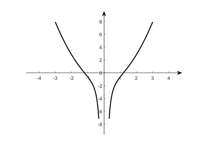
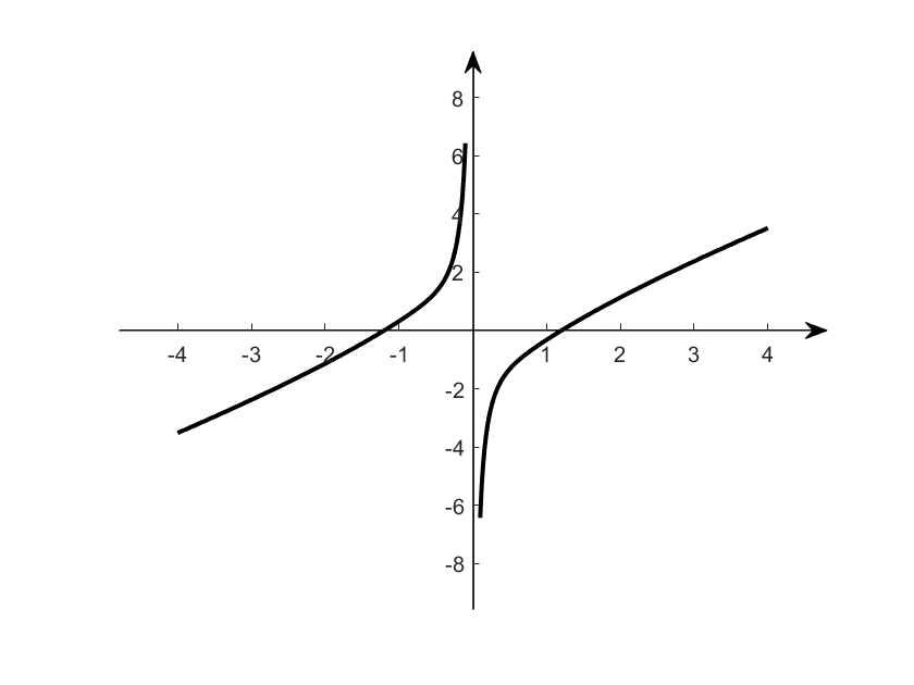
Figure 2. [$b$-KP-II equation] (a) Graph of the map $n\mapsto\kappa\frac{k^{2}(n^{2}-1)}{1+k^{2}}-\frac{\ell^{2}}{n^{2}}$ for $\kappa=2,k=1$ and $\ell=0.8$. The eigenvalues of $\mathcal{K}_{0}(\ell)$ are found by taking $n=q,q\in\mathbb{Z}^{*}$. (b) Graph of the dispersion relation $n\mapsto\nu(n)=n\left(\frac{\kappa}{1+k^{2}}-\frac{\kappa}{1+k^{2}n^{2}}-\frac{\ell^{2}}{n^{2}(1+k^{2}n^{2})}\right)$ for $\kappa=2,k=1$ and $\ell=0.8$. The imaginary parts of the eigenvalues of $\mathcal{A}_{0}(\ell)$ are found by taking $k=n,n\in\mathbb{Z}^{*}$. Notice that the zeros of the two maps are the same.

In contrast to the $b$-KP-I equation, the spectrum of $\mathcal{K}_{0}(\ell)$ contains negative eigenvalues, and the number of these eigenvalues increases with $\ell$.

4.2.2. Spectrum of $\mathcal{A}_{0}(\ell)$

The spectrum of the operator $\mathcal{A}_{0}(\ell)$ acting in $L_{0}^{2}(\mathbb{T})$ is given by (see also Figure 2 (b))

$$\operatorname{spec}_{L_{0}^{2}(\mathbb{T})}\left(\mathcal{A}_{0}(\ell)\right)=\left\{i\nu_{n}(\ell)=in\left(\frac{\kappa}{1+k^{2}}-\frac{\kappa}{1+k^{2}n^{2}}-\frac{\ell^{2}}{n^{2}(1+k^{2}n^{2})}\right)\;:\;n\in\mathbb{Z}^{*}\right\}.$$

Notice that the dispersion relation

$$\nu(n):=n\left(\frac{\kappa}{1+k^{2}}-\frac{\kappa}{1+k^{2}n^{2}}-\frac{\ell^{2}}{n^{2}(1+k^{2}n^{2})}\right)$$

is monotonically increasing on $(-\infty,-1]$ and $[1,\infty)$, so that colliding eigenvalues correspond to Fourier modes with opposite signs. A direct calculation then shows that for any $p,q\in\mathbb{N}^{*}$ the eigenvalues corresponding to the Fourier modes $p$ and $-q$ collide when

$$\ell^{2}=\ell_{p,q}^{2}:=\kappa\frac{pq\left(1+k^{2}p^{2}\right)\left(1+k^{2}q^{2}\right)}{p\left(1+k^{2}p^{2}\right)+q\left(1+k^{2}q^{2}\right)}\left(\frac{p+q}{1+k^{2}}-\frac{p\left(1+k^{2}q^{2}\right)+q\left(1+k^{2}p^{2}\right)}{(1+k^{2}p^{2})(1+k^{2}q^{2})}\right).$$

Moreover, the corresponding eigenvalues of $\mathcal{K}_{0}(\ell)$ have opposite signs, so that any of these collisions may lead to unstable eigenvalues of the operator $\mathcal{A}_{a}(\ell)$.

4.2.3. Long wavelength transverse perturbations

Lemma 4.5.

Assume that $|\ell|$ and $|a|$ are sufficiently small. Recall the definition (4.5) for $\ell_{a}^{2}$. If $\ell^{2}_{a}<0$, then there exists some

$$\ell_{**}^{2}:=-\ell^{2}_{a}+O(a^{4})>0.$$

1. for any $\ell^{2}>\ell_{**}^{2}$, the spectrum of $\mathcal{A}_{a}(\ell)$ is purely imaginary.

2. for any $\ell^{2}<\ell_{**}^{2}$, the spectrum of $\mathcal{A}_{a}(\ell)$ is purely imaginary, except for a pair of simple real eigenvalues with opposite signs.

If $\ell_{a}^{2}>0$, then the spectrum of $\mathcal{A}_{a}(\ell)$ is purely imaginary.

Proof.

Upon replacing $\ell^{2}$ by $-\ell^{2}$ in (4.6), we find that the two eigenvalues satisfy

$$\lambda^{2}=-\frac{\ell^{2}}{(1+k^{2})^{2}}\left[\ell^{2}+\ell^{2}_{a}+O\left(a^{2}\left(\ell^{2}+a^{2}\right)\right)\right].$$

Consequently, we may process as in Theorem 4.1 to get the results. ∎

The parameter regimes indicating the sign of $\ell_{a}^{2}$ is given in Lemma 4.4, which together with Lemma 4.5 provides the spectral stability for the $b$-KP-II case.

5. Non-periodic perturbations for $b$-KP-I: onset of instability

In this section, we will consider the two-dimensional perturbations which are non-periodic (localized or bounded) in the direction of the propagation of the wave. For non-periodic perturbations, we study the invertibility of $\mathcal{T}_{a}(\lambda,\ell)$ in (3) acting in $L^{2}(\mathbb{R})$ or $C_{\textup{bdd}}(\mathbb{R})$ (with domain $H^{4}(\mathbb{R})$ or $C_{\textup{bdd}}^{4}(\mathbb{R})$ ), for $\lambda\in\mathbb{C},\ \Re(\lambda)>0$, and $\ell\in\mathbb{R}\backslash\{0\}$. The notable difference in this case is that $\mathcal{T}_{a}(\lambda,\ell)$ now has bands of continuous spectrum.

5.1. Reformulation and main result

Since the coefficients of $\mathcal{T}_{a}(\lambda,\ell)$ are periodic functions, using Floquet theory, all solutions of $\mathcal{T}_{a}(\lambda,\ell)V=0$ in $L^{2}(\mathbb{R})$ or $C_{\textup{bdd}}(\mathbb{R})$ are of the form $V(z)=\mathrm{e}^{i\xi z}\tilde{V}(z)$ where $\xi\in\left(-\frac{1}{2},\frac{1}{2}\right]$ is the Floquet exponent and $\tilde{V}$ is a $2\pi$-periodic function; see [15] for a similar situation. This replaces the study of invertibility of the operator $\mathcal{T}_{a}(\lambda,\ell)$ in $L^{2}(\mathbb{R})$ or $C_{\textup{bdd}}(\mathbb{R})$ by the study of invertibility of a family of Bloch operators in $L^{2}(\mathbb{T})$ parameterized by the Floquet exponent $\xi$. We present the precise reformulation in the following lemma.

Lemma 5.1.

The linear operator $\mathcal{T}_{a}(\lambda,\ell)$ is invertible in $L^{2}(\mathbb{R})$ if and only if the linear operators

$$\mathcal{T}_{a,\xi}(\lambda,\ell)$$

$$\ =\left(1-k^{2}\left(\partial_{z}+i\xi\right)^{2}\right)\left(\partial_{z}+i\xi\right)\left\{\lambda-c\left(\partial_{z}+i\xi\right)+\left(1-k^{2}\left(\partial_{z}+i\xi\right)^{2}\right)^{-1}\right.$$

$$\ \quad\left.\left(\partial_{z}+i\xi\right)\left[\kappa+(b+1)w-k^{2}w_{zz}-(b-1)k^{2}w_{z}\left(\partial_{z}+i\xi\right)-k^{2}w\left(\partial_{z}+i\xi\right)^{2}\right]\right\}-\sigma\ell^{2}$$

acting in $L^{2}(\mathbb{T})$ with domain $H^{4}_{\textup{per}}(\mathbb{T})$ are invertible for all $\xi\in\left(-\frac{1}{2},\frac{1}{2}\right]$.

We refer to [15, Proposition 1.1] for a detailed proof in the similar situation. The fact that the operators $\mathcal{T}_{a,\xi}(\lambda,\ell)$ act in $L^{2}(\mathbb{T})$ with compactly embedded domain $H^{4}_{\textup{per}}(\mathbb{T})$ implies that these operators have only point spectrum. Noting that $\xi=0$ corresponds to the periodic perturbations which we have already investigated, we would restrict ourselves to the case of $\xi\neq 0$. Thus the operator $\partial_{z}+i\xi$ is invertible in $L^{2}(\mathbb{T})$. Using this, we have the following result.

Lemma 5.2.

The operator $\mathcal{T}_{a,\xi}(\lambda,\ell)$ is not invertible in $L^{2}(\mathbb{T})$ for some $\lambda\in\mathbb{C}$ and $\xi\neq 0$ if and only if $\lambda\in\operatorname{spec}_{L^{2}(\mathbb{T})}\left(\mathcal{A}_{a}(\ell,\xi)\right)$, where

$$\mathcal{A}_{a}(\ell,\xi)$$

$$= \left(\partial_{z}+i\xi\right)\left[c-\left(1-k^{2}\left(\partial_{z}+i\xi\right)^{2}\right)^{-1}\right.$$

$$\left.\left(\kappa+(b+1)w-k^{2}w_{zz}-k^{2}(b-1)w_{z}\left(\partial_{z}+i\xi\right)-k^{2}w\left(\partial_{z}+i\xi\right)^{2}-\sigma\ell^{2}\left(\partial_{z}+i\xi\right)^{-2}\right)\right]$$

$$= \left(\partial_{z}+i\xi\right)\left[1-k^{2}\left(\partial_{z}+i\xi\right)^{2}\right]^{-1}\Big{[}c\left(1-(\partial_{z}+i\xi)^{2}\right)-$$

$$\left.\left(\kappa+(b+1)w-k^{2}w_{zz}-k^{2}(b-1)w_{z}\left(\partial_{z}+i\xi\right)-k^{2}w\left(\partial_{z}+i\xi\right)^{2}-\sigma\ell^{2}\left(\partial_{z}+i\xi\right)^{-2}\right)\right].$$

Note that the operator $\left(\partial_{z}+i\xi\right)^{-1}$ becomes singular as $\xi\rightarrow 0$. Thus the implication from the spectral information of $\mathcal{A}_{a}(\ell,\xi)$ to the invertibility of $\mathcal{T}_{a,\xi}(\lambda,\ell)$ is not uniform in $\xi$. Therefore we will restrict our attention to the case when $|\xi|>\epsilon>0$, and look to detect the onset of instability.

Lemma 5.3.

Assume that $\xi\in\left(-\frac{1}{2},\frac{1}{2}\right]$ and $\xi\neq 0$. Then the spectrum $\operatorname{spec}_{L^{2}(\mathbb{T})}\left(\mathcal{A}_{a}(\ell,\xi)\right)$ is symmetric with respect to the imaginary axis, and $\operatorname{spec}_{L^{2}(\mathbb{T})}\left(\mathcal{A}_{a}(\ell,\xi)\right)=\operatorname{spec}_{L^{2}(\mathbb{T})}\left(-\mathcal{A}_{a}(\ell,-\xi)\right)$.

Proof.

We consider $\mathcal{S}$ to be the reflection through the imaginary axis defined as follows

$$\mathcal{S}\psi(z)=\overline{\psi(-z)},$$

and notice that $\mathcal{A}_{a}(\ell,\xi)$ anti-commutes with $\mathcal{S}$,

$$\left(\mathcal{A}_{a}(\ell,\xi)\mathcal{S}\psi\right)(z)=\mathcal{A}_{a}(\ell,\xi)\left(\overline{\psi(-z)}\right)=-\overline{\left(\mathcal{A}_{a}(\ell,\xi)\psi\right)}(-z)=-\left(\mathcal{S}\mathcal{A}_{a}(\ell,\xi)\right)\psi(z),$$

where we have used the fact that $w$ is an even function. Assume $\mu$ is the eigenvalue of $\mathcal{A}_{a}(\ell,\xi)$ with an associated eigenvector $\varphi$,

$$\mathcal{A}_{a}(\ell,\xi)\varphi=\mu\varphi.$$

then we have

$$\mathcal{A}_{a}(\ell,\xi)\mathcal{S}\varphi=-\mathcal{S}\mathcal{A}_{a}(\ell,\xi)\varphi=-\overline{\mu}\mathcal{S}\varphi.$$

Consequently, $-\overline{\mu}$ is an eigenvalue of $\mathcal{A}_{a}(\ell,\xi)$. This implies that the spectrum of $\mathcal{A}_{a}(\ell,\xi)$ is symmetric with respect to imaginary axis.

Consider $\mathcal{R}$ to be the reflection as follows

$$\mathcal{R}\psi(z)=\psi(-z),$$

then we have

$$\left(\mathcal{A}_{a}(\ell,\xi)\mathcal{R}\right)\psi(z)=\mathcal{A}_{a}(\ell,\xi)\left(\psi(-z)\right)=-\left(\mathcal{A}_{a}(\ell,-\xi)\psi\right)(-z)=-\left(\mathcal{R}\mathcal{A}_{a}(\ell,-\xi)\psi\right)(z).$$

This gives the second property. ∎

From the above lemma, we can without loss of generality assume that $\xi\in\left(0,\frac{1}{2}\right]$. We will study the $L^{2}(\mathbb{T})$-spectra of the linear operators $\mathcal{A}_{a}(\ell,\xi)$ for $|a|$ sufficiently small. It is straightforward to establish the estimate

$$\left\|\mathcal{A}_{a}(\ell,\xi)-\mathcal{A}_{0}(\ell,\xi)\right\|_{H^{1}(\mathbb{T})\rightarrow L^{2}(\mathbb{T})}=O(|a|)$$

as $a\rightarrow 0$ uniformly for $\xi\in\left(0,\frac{1}{2}\right]$ in the operator norm. Therefore, in order to locate the spectrum of $\mathcal{A}_{a}(\ell,\xi)$, we need to determine the spectrum of $\mathcal{A}_{0}(\ell,\xi)$. A simple calculation yields that

$$\mathcal{A}_{0}(\ell,\xi)\mathrm{e}^{inz}=i\omega_{n}(\ell,\xi)\mathrm{e}^{inz},\quad n\in\mathbb{Z},$$ (5.1a)

where

$$\omega_{n}(\ell,\xi)=(n+\xi)\left(\frac{\kappa}{1+k^{2}}-\frac{\kappa}{1+k^{2}(n+\xi)^{2}}-\frac{\sigma\ell^{2}}{(n+\xi)^{2}\left(1+k^{2}(n+\xi)^{2}\right)}\right).$$ (5.1b)

As in the previous section, the linear operator $\mathcal{A}_{0}(\ell,\xi)$ can be decomposed as

$$\mathcal{A}_{0}(\ell,\xi)=J_{\xi}\mathcal{K}_{0}(\ell,\xi),$$

where

$$J_{\xi}:=\left(\partial_{z}+i\xi\right)\left(1-k^{2}\left(\partial_{z}+i\xi\right)^{2}\right)^{-1},$$

and

$$\mathcal{K}_{0}(\ell,\xi):= \left(c_{0}\left(1-(\partial_{z}+i\xi)^{2}\right)-\kappa+\sigma\ell^{2}\left(\partial_{z}+i\xi\right)^{-2}\right).$$

The operator $J_{\xi}$ is skew-adjoint, whereas the operator $\mathcal{K}_{0}(\ell,\xi)$ is self-adjoint. As defined in (4.3), the Krein signature, $K_{n,\xi}$ of an eigenvalue $i\omega_{n}(\ell,\xi)$ in $\operatorname{spec}\left(\mathcal{A}_{0}(\ell,\xi)\right)$ is

$$K_{n,\xi}=\operatorname{sgn}\left(\mu_{n}(\ell,\xi):=\frac{\kappa k^{2}\left((n+\xi)^{2}-1\right)}{1+k^{2}}-\frac{\sigma\ell^{2}}{(n+\xi)^{2}}\right)$$

for $n\in\mathbb{Z}$. Note that we have

$$\omega_{n}(\ell,\xi)=\frac{n+\xi}{1+k^{2}(n+\xi)^{2}}\mu_{n}(\ell,\xi).$$ (5.2)

As explained in the previous section, the $b$-KP-II case is very difficult to analyze, and hence we will mainly focus on the $b$-KP-I equation ($\sigma=-1$).

The main result of this section is the following theorem showing the finite-wavelength transverse spectral instability of the periodic waves for the $b$-KP-I equation under perturbations which are non-periodic in $z$.

Theorem 5.1 (Instability under finite-wavelength transverse perturbation).

Consider $\sigma=-1$. Assume that $\xi\in\left(0,\frac{1}{2}\right]$ and define

$$\begin{split}\ell_{0}^{2}&:=\frac{\kappa k^{2}(1-\xi^{2})\xi^{2}}{\left(1+k^{2}\right)},\\ \ell_{c}^{2}&:=\frac{\kappa k^{2}(1-\xi)^{2}\xi^{2}}{\left(1+k^{2}\right)}\cdot\frac{\left(1+\xi\right)\left[1+k^{2}(1-\xi)^{2}\right]+\left(1+k^{2}\xi^{2}\right)\left(2-\xi\right)}{\left(1-\xi\right)\left[1+k^{2}(1-\xi)^{2}\right]+\left(1+k^{2}\xi^{2}\right)\xi},\end{split}$$ (5.3)

and

$$B:=\left[k^{2}\xi^{2}+(1-b)k^{2}\xi+k^{2}+(b+1)\right]\left[k^{2}\xi^{2}+(b-3)k^{2}\xi+(3-b)k^{2}+(b+1)\right].$$ (5.4)

Therefore we know that $\ell_{0}^{2}{\leq}\ell_{c}^{2}$. Then for $\ell^{2}\geq\ell_{0}^{2}$, we have

1. In the case of $B>0$, for any $|a|$ sufficiently small, there exists $\varepsilon_{a}(\xi)>0$ with

   $$\varepsilon_{a}(\xi):=\xi^{\frac{3}{2}}(1-\xi)^{\frac{3}{2}}\frac{(1+k^{2}\xi^{2})^{\frac{1}{2}}\left(1+k^{2}(1-\xi)^{2}\right)^{\frac{1}{2}}}{(1-\xi)\left[1+k^{2}(1-\xi)^{2}\right]+\xi(1+k^{2}\xi^{2})}B^{\frac{1}{2}}|a|$$ (5.5)

   such that

   1. for $\left|\ell^{2}-\ell_{c}^{2}(\xi)\right|>\varepsilon_{a}(\xi)$, the spectrum of $\mathcal{A}_{a}(\ell,\xi)$ is purely imaginary;

   2. for $\left|\ell^{2}-\ell_{c}^{2}(\xi)\right|<\varepsilon_{a}(\xi)$, the spectrum of $\mathcal{A}_{a}(\ell,\xi)$ is purely imaginary, except for a pair of complex eigenvalues with opposite nonzero real parts.

2. In the case when $B<0$, the spectrum of $\mathcal{A}_{a}(\ell,\xi)$ is purely imaginary.

Remark 5.1.

From Lemma 5.9 we see that the transverse spectral instability holds for $-1\leq b\leq 3$, which covers the well-known examples of CH-KP-I ($b=2$) and DP-KP-I ($b=3$).

The remainder of this subsection aims at proving this theorem, and the main argument is provided in Section 5.4.

5.2. The Krein signature and stability under short-wavelength transverse perturbations

We start the analysis of the spectrum of $\mathcal{A}_{0}(\ell,\xi)$ with the values of $\ell$ away from the origin, $|\ell|>\ell_{0}$, for some $\ell_{0}>0$. Recall that now we take $\sigma=-1$. It is straight forward to verify that

• $K_{n,\xi}=1$ for all $n\in\mathbb{Z}\backslash\{-1,0\}$, $k>0$, and $\xi\in\left(0,\frac{1}{2}\right]$, as

  $$\mu_{n}(\ell,\xi)>\frac{\kappa k^{2}\left((n+\xi)^{2}-1\right)}{1+k^{2}}\geqslant\frac{\kappa k^{2}}{\left(1+k^{2}\right)}\xi(2+\xi);$$

• when $n=-1$, the eigenvalue

  $$\mu_{-1}(\ell,\xi)=\left(\frac{\ell^{2}}{(1-\xi)^{2}}-\frac{\kappa k^{2}\xi(2-\xi)}{\left(1+k^{2}\right)}\right)$$

  is positive when $\ell^{2}>\ell_{-}^{2}$, where $\ell_{-}^{2}:=\frac{\kappa k^{2}\xi(2-\xi)(1-\xi)^{2}}{\left(1+k^{2}\right)}$; it is zero when $\ell^{2}=\ell_{-}^{2}$, and it is negative when $\ell^{2}<\ell_{-}^{2}$;

• when the Fourier mode $n=0$, the eigenvalue

  $$\mu_{0}(\ell,\xi)=\left(\frac{\ell^{2}}{\xi^{2}}-\frac{\kappa k^{2}(1-\xi^{2})}{\left(1+k^{2}\right)}\right)$$

  is positive when $\ell^{2}>\ell_{0}^{2}$, where $\ell_{0}^{2}$ is defined in (5.3); it is zero when $\ell^{2}=\ell_{0}^{2}$, and it is negative when $\ell^{2}<\ell_{0}^{2}$. (see also Figure 3 (a)).

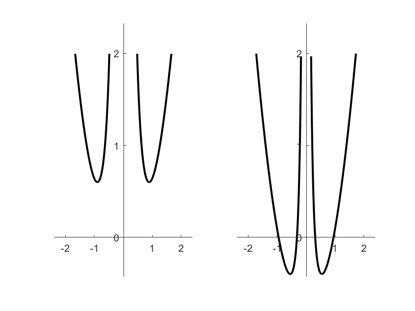
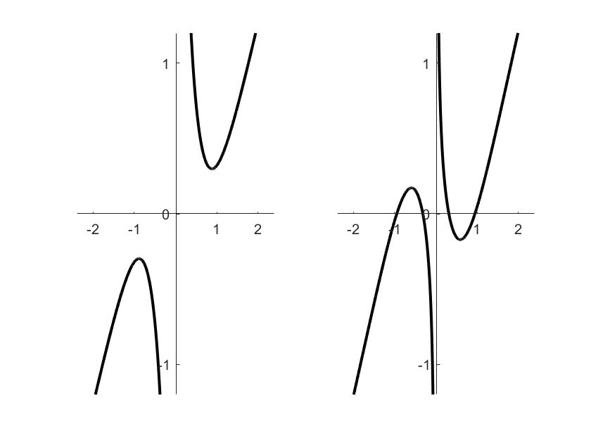
Figure 3. [$b$-KP-I equation] (a) Graph of the map $n\mapsto\frac{\ell^{2}}{n^{2}}-\frac{\kappa k^{2}(1-n^{2})}{1+k^{2}}$ for $\kappa=2,k=1$ and $\ell=0.8$ and $\ell=0.3$ (from left to right). The eigenvalues of $\mathcal{K}_{0}(\ell)$ are found by taking $n=p+\xi,p\in\mathbb{Z}$. (b) Graph of the dispersion relation $n\mapsto n\left(\frac{\kappa}{1+k^{2}}-\frac{\kappa}{1+k^{2}n^{2}}+\frac{\ell^{2}}{n^{2}(1+k^{2}n^{2})}\right)$ for the same values of $\ell,\kappa$ and $k$. The imaginary parts of the eigenvalues of $\mathcal{A}_{0}(\ell)$ are found by taking $n=p+\xi,p\in\mathbb{Z}$. Notice that the zeros of the two maps are the same.

Here

$$\ell_{0}^{2}=\frac{\kappa k^{2}(1-\xi^{2})\xi^{2}}{\left(1+k^{2}\right)}<\ell_{-}^{2}=\frac{\kappa k^{2}(1-\xi)^{2}\xi(2-\xi)}{\left(1+k^{2}\right)},$$

for any $\xi\in\left(0,\frac{1}{2}\right)$, so that the unperturbed operator $\mathcal{K}_{0}(\ell,\xi)$ has positive spectrum for $\ell^{2}>\ell_{-}^{2}$, one negative eigenvalue if $\ell_{0}^{2}\leq\ell^{2}<\ell_{-}^{2}$, and two negative eigenvalues if $\ell^{2}<\ell_{0}^{2}$. The following result is an immediate consequence of these properties and we refer to [16, Lemma 5.4] for a detailed proof in a similar situation.

Lemma 5.4 (Stability under short-wavelength transverse perturbation).

Assume that $\xi\in\left(0,\frac{1}{2}\right]$. For any $\varepsilon_{*}>0$ there exists $a_{*}>0$, such that the spectrum of $\mathcal{A}_{a}(\ell,\xi)$ is purely imaginary, for any $\ell$ and a satisfying $\ell^{2}\geqslant\ell_{-}^{2}+\varepsilon_{*}$ and $|a|\leqslant a_{*}$.

It remains to determine the spectrum of $\mathcal{A}_{a}(\ell,\xi)$ for $0<\ell^{2}<\ell_{-}^{2}+\varepsilon_{*}$. We proceed as in Section 4.1 to decompose the spectrum of $\mathcal{A}_{a}(\ell,\xi)$ into $\sigma_{0}\left(\mathcal{A}_{a}(\ell,\xi)\right)$ containing a minimal number of eigenvalues, and $\sigma_{1}\left(\mathcal{A}_{a}(\ell,\xi)\right)$ for which we argue as in Theorem 4.1 to show that it is purely imaginary.

5.3. Spectral decomposition of $\mathcal{A}_{0}(\ell,\xi)$ for $\ell_{0}^{2}\leq\ell^{2}<\ell_{-}^{2}+\varepsilon_{*}$

Recall that the spectrum of $\mathcal{A}_{0}(\ell,\xi)$ is given in (5.1). The distribution of these eigenvalues on the imaginary axis can be inferred from the study of the dispersion relation (see Figure 3 (b)). The discussion preceding Lemma 5.4 implies that the eigenvalues of $\mathcal{A}_{0}(\ell,\xi)$ that might lead to instability under perturbations are

$$i\omega_{-1}(\ell,\xi),\quad\qquad \ \ell_{0}^{2}\leq\ell^{2}{\leq}\ell_{-}^{2},$$ if

$$i\omega_{-1}(\ell,\xi),\ i\omega_{0}(\ell,\xi), \ 0<\ell^{2}<\ell_{0}^{2}.$$ if

The next step is to separate these eigenvalues from the remaining point spectra, which correspond to the ones with positive Krein signature. Such a separation is possible as long as there are no collisions between these eigenvalues and other ones. The following lemma confirms this lack of collision for transverse perturbations in the finite wave length regime.

Lemma 5.5.

Assume that $\xi\in\left(0,\frac{1}{2}\right]$. The eigenvalues of $\mathcal{A}_{0}(\ell,\xi)$ satisfy

$$\begin{split}\omega_{-1}(\ell,\xi)&=\omega_{0}(\ell,\xi)\quad\text{only when }\ \ell^{2}=\ell_{c}^{2},\\ \omega_{-1}(\ell,\xi)&\neq\omega_{n}(\ell,\xi)\quad\text{for all }\ n\neq 0,-1,1.\end{split}$$ (5.6a)

When $$\ell_{0}^{2}\leq\ell^{2}{\leq}\ell_{-}^{2}$$ it further holds that

$$\omega_{-1}(\ell,\xi)\neq\omega_{n}(\ell,\xi)\quad\text{for all }\ n\neq 0,-1.$$ (5.6b)

Proof.

Define the collision function

$$F_{n}(\ell^{2},\xi):= \ \omega_{n}(\ell,\xi)-\omega_{-1}(\ell,\xi)=\frac{1-\xi}{1+k^{2}(1-\xi)^{2}}\mu_{-1}(\ell,\xi)+\frac{n+\xi}{1+k^{2}(n+\xi)^{2}}\mu_{n}(\ell,\xi)$$

$$= \ \frac{\kappa k^{2}}{1+k^{2}}\left[\frac{(1-\xi)\left[(1-\xi)^{2}-1\right]}{1+k^{2}(1-\xi)^{2}}+\frac{(n+\xi)\left[(n+\xi)^{2}-1\right]}{1+k^{2}(n+\xi)^{2}}\right]+$$

$$\ \ell^{2}\left[\frac{1}{(1-\xi)\left[1+k^{2}(1-\xi)^{2}\right]}+\frac{1}{(n+\xi)\left[1+k^{2}(n+\xi)^{2}\right]}\right]$$

$$=: \ G_{n}(\xi)+\ell^{2}H_{n}(\xi).$$

Clearly $F_{n}$ is linear in $\ell^{2}$. From the previous discussion we see that

$$\omega_{-1}(\ell,\xi){\geq}0,\qquad\text{and}\qquad\omega_{n}(\ell,\xi)\left\{\begin{aligned} &\geq 0,\quad\text{for}\;n\geqslant 0,\\ &<0,\quad\text{for}\;n\leq-2.\end{aligned}\right.$$

Thus only $\omega_{n}(\ell,\xi)$ with $n\geq 0$ is possible to collide with $\omega_{-1}(\ell,\xi)$.

When $n=0$, we consider solving

$$F_{0}(\ell^{2})=\frac{1-\xi}{1+k^{2}(1-\xi)^{2}}\mu_{-1}(\ell,\xi)+\frac{\xi}{1+k^{2}\xi}\mu_{0}(\ell,\xi)=0$$

for $\ell^{2}$. Since both $\mu_{-1}(\ell,\xi)$ and $\mu_{0}(\ell,\xi)$ are linear increasing functions in $\ell^{2}$, so is $F_{0}(\ell^{2},\xi)$. Also we have $F_{0}(\ell_{0}^{2},\xi)<0$ and $F_{0}(\ell_{-}^{2},\xi)>0$ for $\xi\in\left(0,\frac{1}{2}\right)$. Hence for any given $\xi\in\left(0,\frac{1}{2}\right)$ there exists a unique $\ell_{c}^{2}\in(\ell_{0}^{2},\ell_{-}^{2})$ such that $F(\ell_{c}^{2},\xi)=0$. Explicit computation reveals that $\ell_{c}^{2}$ is given in (5.3). For the case $\xi=\frac{1}{2}$, we have $\ell_{c}^{2}=\ell_{0}^{2}=\ell_{-}^{2}$, and hence $\omega_{-1}(\ell_{c}^{2},\xi)=\omega_{0}(\ell_{c}^{2},\xi)=0$. This proves the first part of (5.6).

Now for $n\geq 1$, the function $G_{n}(\xi)$ is related to the function

$$f(x)=\frac{(1-\xi)\left[(1-\xi)^{2}-1\right]}{1+k^{2}(1-\xi)^{2}}+\frac{(x+\xi)\left[(x+\xi)^{2}-1\right]}{1+k^{2}(x+\xi)^{2}},$$

which is increasing for $|x+\xi|>\frac{1}{\sqrt{3}}$. Moreover,

$$f(2)=\frac{\left(6+9\xi+9\xi^{2}\right)+3k^{2}\left(1-\xi-\xi^{2}\right)\left(2+\xi\right)\left(1-\xi\right)}{\left(1+k^{2}(2+\xi)^{2}\right)\left(1+k^{2}(1-\xi)^{2}\right)}>0.$$

Therefore $\omega_{-1}(\ell,\xi)$ does not collide with $\omega_{n}(\ell,\xi)$ for $n\geq 2$, and hence it suffices to consider the case when $n=1$. Direct computation shows that

$$G_{1}(\xi)=\frac{\kappa k^{2}}{1+k^{2}}\frac{2\xi^{2}\left[3-k^{2}(1-\xi^{2})\right]}{\left[1+k^{2}(1-\xi)^{2}\right]\left[1+k^{2}(1+\xi)^{2}\right]},$$

and

$$G_{1}(\xi)<0\quad\text{only if}\quad k^{2}>\frac{3}{1-\xi^{2}}.$$

In this case, solving $F_{1}(\ell^{2},\xi)=0$ we find that the unique solution for $\ell^{2}$ is

$$\ell^{2}=\frac{\kappa k^{2}(1-\xi^{2})\xi^{2}}{\left(1+k^{2}\right)}\cdot\frac{k^{2}(1-\xi^{2})-3}{1+k^{2}\left(1+3\xi^{2}\right)}<\frac{\kappa k^{2}(1-\xi^{2})\xi^{2}}{\left(1+k^{2}\right)}=\ell_{0}^{2}.$$

Therefore the second part of (5.6) is proved. ∎

From the above lemma it follows that

Lemma 5.6.

Given $\xi\in\left(0,\frac{1}{2}\right]$, there exist $\varepsilon_{*}>0$ and $c_{*}>0$ such that

1. for any $\ell$ satisfying $\ell_{c}^{2}+\varepsilon_{*}<\ell^{2}<\ell_{-}^{2}+\varepsilon_{*}$, the spectrum of $\mathcal{A}_{0}(\ell,\xi)$ decomposes as

   $$\sigma\left(\mathcal{A}_{0}(\ell,\xi)\right)=\left\{i\omega_{-1}(\ell,\xi)\right\}\cup\sigma_{1}\left(\mathcal{A}_{0}(\ell,\xi)\right),$$

   with $\operatorname{dist}\left(i\omega_{-1}(\ell,\xi),\sigma_{1}\left(\mathcal{A}_{0}(\ell,\xi)\right)\right)\geqslant c_{*}>0$;

2. for any $\ell$ satisfying $\ell_{0}^{2}\leq\ell^{2}\leqslant\ell_{c}^{2}+\varepsilon_{*}$, the spectrum of $\mathcal{A}_{0}(\ell,\xi)$ decomposes as

   $$\sigma\left(\mathcal{A}_{0}(\ell,\xi)\right)=\left\{i\omega_{-1}(\ell,\xi),i\omega_{0}(\ell,\xi)\right\}\cup\sigma_{1}\left(\mathcal{A}_{0}(\ell,\xi)\right),$$

   with $\operatorname{dist}\left(\left\{i\omega_{-1}(\ell,\xi),i\omega_{0}(\ell,\xi)\right\},\sigma_{1}\left(\mathcal{A}_{0}(\ell,\xi)\right)\right)\geqslant c_{*}>0$.

Continuity arguments show that for sufficiently small $a$, this decomposition persists for the operator $\mathcal{A}_{a}(\ell,\xi)$, and we argue as in Section 4.1.2 to locate the spectrum of $\mathcal{A}_{a}(\ell,\xi)$.

5.4. Spectrum of $\mathcal{A}_{a}(\ell,\xi)$ for $\ell_{0}^{2}\leq\ell^{2}<\ell_{-}^{2}+\varepsilon_{*}$

Let us start with the case $\ell_{c}^{2}+\varepsilon_{*}<\ell^{2}<\ell_{-}^{2}+\varepsilon_{*}$. The following lemma asserts that for $\ell$ in this range the spectrum of $\mathcal{A}_{a}(\ell,\xi)$ is purely imaginary. The argument follows in a similar way as that of [16, Lemma 5.6], and hence we omit the proof here.

Lemma 5.7.

Assume that $\xi\in\left(0,\frac{1}{2}\right]$. There exist $\varepsilon_{*}>0$ and $a_{*}>0$ such that the spectrum of $\mathcal{A}_{a}(\ell,\xi)$ is purely imaginary, for any $\ell$ and a satisfying $\ell_{c}^{2}+\varepsilon_{*}<\ell^{2}<\ell_{-}^{2}+\varepsilon_{*}$ and $|a|\leqslant a_{*}$.

Next we consider the spectrum of $\mathcal{A}_{a}(\ell,\xi)$ for $\ell_{0}^{2}\leq\ell^{2}\leqslant\ell_{c}^{2}+\varepsilon_{*}$. From Section 5.3 we know that the two eigenvalues of $\mathcal{A}_{0}(\ell,\xi)$ corresponding to the Fourier modes $n=-1$ and $n=0$ collide at $\ell^{2}=\ell_{c}^{2}$. Using perturbation arguments we prove in the following that for $a$ sufficiently small and $\ell$ close to the value $\ell_{c}$, the linearized operator $\mathcal{A}_{a}(\ell,\xi)$ will continue to accommodate a pair of unstable eigenvalues. This, together with the definition of instability, proves Theorem 5.1.

Lemma 5.8.

Assume that $\xi\in\left(0,\frac{1}{2}\right]$ and recall $B$ in (5.4). In the case of $B>0$, there exist constants $\varepsilon_{*},a_{*}>0$, and $\varepsilon_{a}(\xi)$ as defined in (5.5) with $\varepsilon_{a}(\xi)<\varepsilon_{*}$, such that if $\ell_{0}^{2}\leq\ell^{2}\leqslant\ell_{c}^{2}+\varepsilon_{*}$ and

1. $\left|\ell^{2}-\ell_{c}^{2}\right|>\varepsilon_{a}(\xi)$, then the spectrum of $\mathcal{A}_{a}(\ell,\xi)$ is purely imaginary;

2. $\left|\ell^{2}-\ell_{c}^{2}\right|<\varepsilon_{a}(\xi)$ then the spectrum of $\mathcal{A}_{a}(\ell,\xi)$ is purely imaginary, except for a pair of complex eigenvalues with opposite nonzero real parts.

In the case $B<0$, the spectrum of $\mathcal{A}_{a}(\ell,\xi)$ is purely imaginary for $\ell_{0}^{2}\leq\ell^{2}\leqslant\ell_{c}^{2}+\varepsilon_{*}$.

Proof.

The spectrum of $\mathcal{A}_{a}(\ell,\xi)$ can be decomposed as

$$\sigma\left(\mathcal{A}_{a}(\ell,\xi)\right)=\sigma_{0}\left(\mathcal{A}_{a}(\ell,\xi)\right)\cup\sigma_{1}\left(\mathcal{A}_{a}(\ell,\xi)\right),$$

where $\sigma_{1}\left(\mathcal{A}_{a}(\ell,\xi)\right)$ is purely imaginary, and $\sigma_{0}\left(\mathcal{A}_{a}(\ell,\xi)\right)$ consists of two eigenvalues which are the continuation of the eigenvalues $i\omega_{-1}(\ell,\xi)$ and $i\omega_{0}(\ell,\xi)$ for small $a$. Choosing $\varepsilon_{*}$ and $a_{*}$ sufficiently small, such decomposition persists for any $\ell_{0}^{2}\leq\ell^{2}\leqslant\ell_{c}^{2}+\varepsilon_{*}$ and $|a|\leqslant a_{*}$. Therefore what remains to check are the location of the two eigenvalues in $\sigma_{0}\left(\mathcal{A}_{a}(\ell,\xi)\right)$.

From Lemma 5.5 we know that for any $\ell_{0}^{2}\leq\ell^{2}\leqslant\ell_{c}^{2}+\varepsilon_{*}$ such that $\ell$ outside a neighborhood of $\ell_{c}$, the two eigenvalues $i\omega_{-1}(\ell,\xi)$ and $i\omega_{0}(\ell,\xi)$ are simple and there exists $c_{0}>0$ such that

$$\left|i\omega_{-1}(\ell,\xi)-i\omega_{0}(\ell,\xi)\right|\geqslant c_{0}.$$

For $a$ sufficiently small, the simplicity of this pair of eigenvalues continues to hold into the spectrum of $\mathcal{A}_{a}(\ell,\xi)$. As the spectrum of $\mathcal{A}_{a}(\ell,\xi)$ is symmetric with respect to the imaginary axis, each of these eigenvalues of $\mathcal{A}_{a}(\ell,\xi)$ is purely imaginary for any $\ell$ outside some neighborhood of $\ell_{c}$.

We will proceed as in the proof of Theorem 4.1 to locate $\sigma_{0}\left(\mathcal{A}_{a}(\ell,\xi)\right)$ for $\ell$ close to $\ell_{c}$. We compute successively a basis for the two-dimensional spectral subspace associated with $\sigma_{0}\left(\mathcal{A}_{a}(\ell,\xi)\right)$, the $2\times 2$ matrix $M_{a}(\ell,\xi)$ representing the action of $\mathcal{A}_{a}(\ell,\xi)$ on this basis, and the eigenvalues of this matrix.

At $a=0$, the basis vectors are chosen to be the two eigenvectors associated with the eigenvalues $i\omega_{0}(\ell,\xi)$ and $i\omega_{-1}(\ell,\xi)$,

$$\xi_{0}^{0}(\ell,\xi)=1,\quad\xi_{0}^{1}(\ell,\xi)=e^{-iz}$$

At order $a$, we take $\ell=\ell_{c}$, and proceed as the computation in the proof of Theorem 4.1 to find

$$M_{a}\left(\ell_{c},\xi\right)= \left(\begin{array}[]{cc}i\omega_{0}\left(\ell_{c},\xi\right)&-\frac{i}{2}\frac{(\xi-1)\left(k^{2}\xi^{2}+(1-b)k^{2}\xi+k^{2}+(b+1)\right)}{1+k^{2}(\xi-1)^{2}}a\\ -\frac{i}{2}\frac{\xi\left(k^{2}\xi^{2}+(b-3)k^{2}\xi+(3-b)k^{2}+(b+1)\right)}{1+k^{2}\xi^{2}}a&i\omega_{-1}\left(\ell_{c},\xi\right)\end{array}\right)$$

$$+O\left(a^{2}\right).$$

Together with the expression of $M_{0}(\ell,\xi)$, this yields that

$$M_{a}\left(\ell,\xi\right)= \left(\begin{array}[]{cc}i\omega_{0}\left(\ell_{c},\xi\right)+i\frac{\varepsilon}{\xi(1+k^{2}\xi^{2})}&-\frac{i}{2}\frac{(\xi-1)\left[k^{2}\xi^{2}+(1-b)k^{2}\xi+k^{2}+(b+1)\right]}{1+k^{2}(\xi-1)^{2}}a\\ \\ -\frac{i}{2}\frac{\xi\left[k^{2}\xi^{2}+(b-3)k^{2}\xi+(3-b)k^{2}+(b+1)\right]}{1+k^{2}\xi^{2}}a&i\omega_{-1}\left(\ell_{c},\xi\right)+i\frac{\varepsilon}{(\xi-1)\left[1+k^{2}(\xi-1)^{2}\right]}\end{array}\right)$$

$$+O\left(a^{2}+|a\varepsilon|\right),$$

with $\varepsilon=\ell^{2}-\ell_{c}^{2}$. Recall the definition of $\ell_{c}^{2}$ in (5.3), and the colliding eigenvalues

$$\omega_{0}\left(\ell_{c},\xi\right)=\omega_{-1}\left(\ell_{c},\xi\right)=\frac{2\kappa k^{2}\xi(1-\xi)(1-2\xi)}{\left(1+k^{2}\right)\left\{\left(1-\xi\right)\left[1+k^{2}(1-\xi)^{2}\right]+\left(1+k^{2}\xi^{2}\right)\xi\right\}}=:\omega_{*}(\xi).$$

Seeking eigenvalues $\lambda$ of the form

$$\lambda=i\omega_{*}(\xi)+iX,$$

we find that $X$ is root of the polynomial

$$P(X)= X^{2}-X\left(\frac{\varepsilon}{\xi(1+k^{2}\xi^{2})}+\frac{\varepsilon}{(\xi-1)\left(1+k^{2}(\xi-1)^{2}\right)}+O\left(a^{2}+|a\varepsilon|\right)\right)$$

$$-\frac{a^{2}}{4}\left(\frac{(\xi-1)\left(k^{2}\xi^{2}+(1-b)k^{2}\xi+k^{2}+(b+1)\right)}{1+k^{2}(\xi-1)^{2}}\right)$$

$$\quad\ \cdot\left(\frac{\xi\left(k^{2}\xi^{2}+(b-3)k^{2}\xi+(3-b)k^{2}+(b+1)\right)}{1+k^{2}\xi^{2}}\right)$$

$$+\frac{\varepsilon^{2}}{\xi(\xi-1)(1+k^{2}\xi^{2})\left(1+k^{2}(\xi-1)^{2}\right)}+O\left(a^{2}|\varepsilon|+|a|\varepsilon^{2}+|a|^{3}\right).$$

A direct computation shows that the discriminant of this polynomial $P(X)$ is

$$\begin{split}\Delta_{a}(\varepsilon,\xi)=&\ \varepsilon^{2}\left[\frac{1}{\xi(1+k^{2}\xi^{2})}+\frac{1}{(1-\xi)\left[1+k^{2}(1-\xi)^{2}\right]}\right]^{2}\\ &\ -\frac{\xi(1-\xi)B}{(1+k^{2}\xi^{2})\left[1+k^{2}(1-\xi)^{2}\right]}a^{2}+O\left(|\varepsilon|a^{2}+\varepsilon^{2}|a|+|a|^{3}\right),\end{split}$$

where $B$ is defined in (5.4).

In the case when $B>0$, we can define

$$\varepsilon_{a}(\xi):=\xi^{\frac{3}{2}}(1-\xi)^{\frac{3}{2}}\frac{(1+k^{2}\xi^{2})^{\frac{1}{2}}\left(1+k^{2}(1-\xi)^{2}\right)^{\frac{1}{2}}}{(1-\xi)\left[1+k^{2}(1-\xi)^{2}\right]+\xi(1+k^{2}\xi^{2})}B^{\frac{1}{2}}\cdot|a|>0.$$

Therefore for any $a$ sufficiently small we have $\Delta_{a}(\varepsilon,\xi)\geq 0$ when $|\varepsilon|>\varepsilon_{a}(\xi)$ and $\Delta_{a}(\varepsilon,\xi)<0$ when $|\varepsilon|<\varepsilon_{a}(\xi)$. This implies that, for $\ell_{0}^{2}\leq\ell^{2}\leq\ell_{c}^{2}+\varepsilon_{*}$, the two eigenvalues of $\mathcal{A}_{a}(\ell,\xi)$ are purely imaginary when $\left|\ell^{2}-\ell_{c}^{2}\right|>\varepsilon_{a}(\xi)$, and complex, with opposite nonzero real parts when $\left|\ell^{2}-\ell_{c}^{2}\right|<\varepsilon_{a}(\xi)$.

In the case when $B<0$, we have $\Delta_{a}(\varepsilon,\gamma)>0$, and this implies that the two eigenvalues of $\mathcal{A}_{a}(\ell,\xi)$ are purely imaginary for $\ell_{0}^{2}\leq\ell^{2}\leq\ell_{c}^{2}+\varepsilon_{*}$. ∎

For $\xi\in(0,\frac{1}{2}]$, we list the cases of $B>0$ and $B<0$ in the following lemma and the detailed discussion is given in the Appendix B.

Lemma 5.9.

$B>0$ is valid for the following cases:

1. $-1\leq b\leq 3$;

2. $b<-1$, $\xi=\frac{1}{2}$, $k^{2}\neq\frac{-4(1+b)}{7-2b}$;

3. $b<-1$, $\xi\in(0,\frac{1}{2})$, $k^{2}>\frac{-(1+b)}{\xi^{2}+(1-b)\xi+1}$ or $k^{2}<\frac{-(1+b)}{\xi^{2}+(b-3)\xi+(3-b)}$;

4. $b>3$, $k^{2}\leq\frac{4}{b-3}$;

5. $3<b\leq\frac{7}{2}$, $\xi=\frac{1}{2}$, $k^{2}>\frac{4}{b-3}$;

6. $b>\frac{7}{2}$, $\xi=\frac{1}{2}$, $k^{2}>\frac{4}{b-3}$ and $k^{2}\neq\frac{-4(1+b)}{7-2b}$;

7. $3<b\leq\frac{\xi^{2}-3\xi+3}{1-\xi}$, $\xi\in(0,\frac{1}{2})$;

8. $3<\frac{\xi^{2}-3\xi+3}{1-\xi}<b\leq\frac{\xi^{2}+\xi+1}{\xi}$, $\xi\in(0,\frac{1}{2})$, $\frac{4}{b-3}<k^{2}<\frac{-(1+b)}{\xi^{2}+(b-3)\xi+(3-b)}$;

9. $b>\frac{\xi^{2}+\xi+1}{\xi}>3$, $\xi\in(0,\frac{1}{2})$, $k^{2}>\frac{-(1+b)}{\left(\xi^{2}+(1-b)\xi+1\right)}$ or $\frac{4}{b-3}<k^{2}<\frac{-(1+b)}{\xi^{2}+(b-3)\xi+(3-b)}$.

$B<0$ when one of the following cases occurs:

1. $b<-1$, $\xi\in(0,\frac{1}{2})$, $\frac{-(1+b)}{\xi^{2}+(1-b)\xi+1}<k^{2}<\frac{-(1+b)}{\xi^{2}+(b-3)\xi+(3-b)}$;

2. $3<\frac{\xi^{2}-3\xi+3}{1-\xi}<b\leq\frac{\xi^{2}+\xi+1}{\xi}$, $\xi\in(0,\frac{1}{2})$, $k^{2}>\frac{-(1+b)}{\xi^{2}+(b-3)\xi+(3-b)}$;

3. $b>\frac{\xi^{2}+\xi+1}{\xi}>3$, $\xi\in(0,\frac{1}{2})$, $\frac{-(1+b)}{\xi^{2}+(b-3)\xi+(3-b)}<k^{2}<\frac{-(1+b)}{\left(\xi^{2}+(1-b)\xi+1\right)}$.

5.5. Discussion for long-wavelength transverse perturbations $0<\ell^{2}<\ell_{0}^{2}$

In contrast to case when $\ell^{2}\geq\ell_{0}^{2}$, for long-wavelength transverse perturbations $0<\ell^{2}<\ell_{0}^{2}$, the collision dynamics of the eigenvalues become much harder to track. In fact, it is possible that infinitely many pairs of eigenvalues collide with each other. What we find is that, in order to eliminate these collisions, an additional condition on the longitudinal wavelength is needed. The detailed discussion is provided below.

The collision between $\omega_{-1}$ and $\omega_{n}$ is studied in Lemma 5.5. So we consider the collision between $\omega_{0}$ and $\omega_{n}$ described by the function

$$\begin{split}\tilde{F}_{n}(\ell^{2},\xi):=&\ \omega_{n}(\ell,\xi)-\omega_{0}(\ell,\xi)\\ =&\ \frac{\kappa k^{2}}{1+k^{2}}\left[\frac{\xi\left(1-\xi^{2}\right)}{1+k^{2}\xi^{2}}+\frac{(n+\xi)\left[(n+\xi)^{2}-1\right]}{1+k^{2}(n+\xi)^{2}}\right]+\\ &\ \ell^{2}\left[-\frac{1}{\xi\left(1+k^{2}\xi^{2}\right)}+\frac{1}{(n+\xi)\left[1+k^{2}(n+\xi)^{2}\right]}\right]\\ =:&\ \tilde{G}_{n}(\xi)+\ell^{2}\tilde{H}_{n}(\xi).\end{split}$$ (5.7)

We can also write $\tilde{F}_{n}(\ell^{2},\xi)$ as

$$\tilde{F}_{n}(\ell^{2},\xi)=\frac{\ell_{0}^{2}-\ell^{2}}{\xi\left(1+k^{2}\xi^{2}\right)}+\frac{{\alpha}(n+\xi)^{2}\left[(n+\xi)^{2}-1\right]+\ell^{2}}{(n+\xi)\left[1+k^{2}(n+\xi)^{2}\right]},$$ (5.8)

where ${\alpha}:=\frac{\kappa k^{2}}{1+k^{2}}$. The first term in the right-hand side of (5.8) is positive in the range of $\ell$ considered here. For $n\geq 1$, the second term is clearly positive. So we consider the case when $n\leq-2$. Define the function

$$g(x):=\frac{\ell^{2}+{\alpha}x^{2}(x^{2}-1)}{x(1+k^{2}x^{2})}\qquad\text{for}\quad x\leq-\frac{3}{2}.$$

Then from the estimate that

$$\ell^{2}<\ell_{0}^{2}={\alpha}\xi^{2}(1-\xi^{2}),\quad\text{and}\qquad\xi^{2}(1-\xi^{2})<\frac{1}{4},$$

we have

$$g^{\prime}(x)= \ \frac{{\alpha}\left(k^{2}x^{6}+k^{2}x^{4}+3x^{4}-x^{2}\right)-\ell^{2}(3k^{2}x^{2}+1)}{x^{2}(1+k^{2}x^{2})^{2}}$$

$$\geq \ \frac{{\alpha}\left[k^{2}x^{6}+k^{2}x^{4}+3x^{4}-x^{2}-\xi^{2}(1-\xi^{2})(3k^{2}x^{2}+1)\right]}{x^{2}(1+k^{2}x^{2})^{2}}>0,\quad\text{for}\quad x\leq-\frac{3}{2}.$$

Therefore we see that the second term in the last equality of (5.8) is increasing in $n$ for $n\leq-2$, that is, $\tilde{F}_{n}(\ell^{2},\xi)\leq\tilde{F}_{-2}(\ell^{2},\xi)$ for $n\leq-2$.

Looking at (5.7) we find the $\tilde{H}_{n}(\xi)<0$ when $n\leq-2$. Explicit computation reveals that

$$\tilde{G}_{-2}(\xi)=\frac{2\alpha(1-\xi)^{2}\left[k^{2}\xi(2-\xi)-3\right]}{(1+k^{2}\xi^{2})\left[1+k^{2}(\xi-2)^{2}\right]}.$$

In fact we have

$$\frac{1}{2}\tilde{F}_{-2}(\ell^{2},\xi)=\frac{\left(1+k^{2}\left[1+3(1-\xi)^{2}\right]\right)\ell^{2}-\left[k^{2}\xi(2-\xi)-3\right]\ell_{-}^{2}}{\xi(\xi-2)(1+k^{2}\xi^{2})\left[1+k^{2}(\xi-2)^{2}\right]}.$$

Therefore we have

$$k^{2}\xi(2-\xi)-3\leq 0\quad\Rightarrow\quad\tilde{F}_{-2}(\ell^{2},\xi)<0\quad\Rightarrow\quad\tilde{F}_{n}(\ell^{2},\xi)<0\text{ for all }n\leq-2.$$

Thus we find that for

$$k^{2}\leq\frac{3}{\xi(2-\xi)},\quad\Rightarrow\quad\omega_{0}(\ell,\xi)\neq\omega_{n}(\ell,\xi)\ \text{ for all }n\neq 0,-1.$$ (5.9)

To summarize, we have the following

Lemma 5.10.

Assume that $\xi\in\left(0,\frac{1}{2}\right]$ and $0<\ell^{2}<\ell_{0}^{2}$. For $k^{2}\leq 4$ we have $\omega_{0}(\ell,\xi)\neq\omega_{n}(\ell,\xi)$ for all $n\neq 0$ and for $k^{2}\leq 3$ we have $\omega_{-1}(\ell,\xi)\neq\omega_{n}(\ell,\xi)$ for all $n\neq-1$.

Proof.

The above discussion leads to (5.9). Since $0<\xi\leq\frac{1}{2}$, we know that $\frac{3}{\xi(2-\xi)}\geq 4$ and $\frac{3}{1-\xi^{2}}>3$. Moreover, the calculation in Lemma 5.5 indicates that $\omega_{0}(\ell,\xi)=\omega_{-1}(\ell,\xi)$ only for $\ell^{2}=\ell_{c}^{2}\geq\ell_{0}^{2}$ and for $0<\ell^{2}<\ell_{0}^{2}$ and $k^{2}\leq\frac{3}{1-\xi^{2}}$, $\omega_{-1}(\ell,\xi)\neq\omega_{n}(\ell,\xi)$ for all $n\neq-1$. Thus the proof of the lemma is complete. ∎

From this lemma we may extend the stability part of Theorem 5.1 to the regime of long-wavelength transverse perturbation, provided that the longitudinal wavelength is bounded below.

Proposition 5.1.

If $k^{2}\leq 3$, then the results in (I) and (II) parts of Theorem 5.1 hold for all $\ell^{2}>0$.

Appendix A Small-amplitude expansion

In this section, we give the details on small-amplitude expansion of (2.1). Since $w$ and $c$ depend analytically on $a$ for $|a|$ sufficiently small and since $c$ is even in $a$, we write that

$$w(k,a)(z):=a\cos z+a^{2}w_{2}(z)+a^{3}w_{3}(z)+O\left(a^{4}\right)$$

and

$$c(k,a):=c_{0}(k)+a^{2}c_{2}+O\left(a^{4}\right)$$

as $a\rightarrow 0$, where $w_{2},w_{3},$ . . . are even and $2\pi$-periodic in $z$. Substituting these into (2.2), at the order of $a^{2}$, we gather that

$$\left(\kappa-c_{0}\right)w_{2}+\frac{\kappa}{1+k^{2}}k^{2}\partial_{z}^{2}w_{2}+\frac{(b+1)}{2}\cos^{2}z+k^{2}\cos^{2}z-\frac{(b-1)}{2}k^{2}\sin^{2}z=0,$$

which is equivalent to

$$\frac{\kappa k^{2}}{1+k^{2}}w_{2}+\frac{\kappa k^{2}}{1+k^{2}}\partial^{2}_{z}w_{2} =\frac{(b-1)}{2}k^{2}\sin^{2}z-\left(\frac{(b+1)}{2}+k^{2}\right)\cos^{2}z$$

$$=\frac{(b-1)}{4}k^{2}(1-\cos 2z)-\left(\frac{(b+1)+2k^{2}}{4}\right)\left(\cos 2z+1\right).$$

Then we get that

$$\frac{\kappa k^{2}}{1+k^{2}}(w_{2}+\partial^{2}_{z}w_{2})=-\frac{(b+1)+(3-b)k^{2}}{4}-\frac{(b+1)(1+k^{2})}{4}\cos 2z.$$ (A.1)

A straightforward calculation then reveals that

$$w_{2}=\frac{\left(1+k^{2}\right)}{4\kappa k^{2}}\left[\frac{(b+1)(k^{2}+1)}{3}\cos 2z+\left((b-3)k^{2}+(b+1)\right)\right].$$ (A.2)

At the order of $a^{3}$,

$$\left(\kappa-c_{0}\right)w_{3}-c_{2}\cos z+c_{0}k^{2}\partial_{z}^{2}w_{3}-c_{2}k^{2}\cos z+{(b+1)}\cos zw_{2}$$

$$-k^{2}\left(\cos z\partial_{z}^{2}w_{2}-w_{2}\cos z\right)+{(b-1)}k^{2}\sin z\partial_{z}w_{2}=0,$$

which is equivalent to

$$\frac{\kappa k^{2}}{1+k^{2}}\left(w_{3}+\partial_{z}^{2}w_{3}\right)= -{(b+1)}\cos zw_{2}+c_{2}\left(1+k^{2}\right)\cos z$$ (A.3)

$$+k^{2}\cos z\left(\partial_{z}^{2}w_{2}-w_{2}\right)-{(b-1)}k^{2}\sin z\partial_{z}w_{2}.$$

From (A.2), we get that

$$\partial_{z}^{2}w_{2}-w_{2}=\frac{1+k^{2}}{4\kappa k^{2}}\left[-\frac{5(b+1)}{3}\left(k^{2}+1\right)\cos 2z+\left((3-b)k^{2}+(b+1)\right)\right],$$

which helps us to get that

$$k^{2}\cos z\left(\partial_{z}^{2}w_{2}-w_{2}\right)-(b-1)k^{2}\sin z\partial_{z}w_{2}$$

$$=k^{2}\frac{1+k^{2}}{2\kappa k^{2}}\left[-\frac{5(b+1)}{6}\left(k^{2}+1\right)\cos 2z\cos z+\left(\frac{(3-b)k^{2}+(b+1)}{2}\right)\cos z\right.$$

$$\quad\left.+\frac{b^{2}-1}{3}\left(k^{2}+1\right)\sin z\sin 2z\right]$$

$$=\frac{1+k^{2}}{2\kappa}\left[\frac{b^{2}-1}{3}\left(k^{2}+1\right)\cos(2z-z)-\frac{(b+1)(2b+1)}{6}\left(k^{2}+1\right)\cos 2z\cos z\right.$$

$$\quad\left.+\left(\frac{(3-b)k^{2}+(b+1)}{2}\right)\cos z\right]$$

$$=\frac{1+k^{2}}{2\kappa}[\left(3k^{2}+5\right)\cos z-7\left(k^{2}+1\right)\cos 2z\cos z].$$

Then the right hand side of (A.3) equals to

$$\frac{1+k^{2}}{2\kappa}{\left[\frac{k^{2}(2b^{2}-3b+7)+(2b+1)(b+1)}{6}\cos z-\frac{(b+1)(2b+3)}{6}\left(k^{2}+1\right)\cos 2z\cos z\right.}$$

$$\qquad\quad\left.-\frac{(b+1)^{2}}{6k^{2}}\left(k^{2}+1\right)\cos 2z\cos z-\frac{(b+1)\left(b(k^{2}-1)-(3k^{2}+1)\right)}{2k^{2}}\cos z+2\kappa c_{2}\cos z\right]$$

$$=-\frac{1+k^{2}}{2\kappa}\left[\frac{b+1}{6}\left((2b+3)+\frac{(b+1)}{k^{2}}\right)\left(k^{2}+1\right)\cos 2z\cos z\right.$$

$$\quad\left.-\left(\frac{k^{4}(2b^{2}-3b+7)-k^{2}(b+1)(b-10)+3(b+1)^{2}}{6k^{2}}+2\kappa c_{2}\right)\cos z\right].$$

Noting that

$$\cos 3\alpha=2\cos 2\alpha\cos\alpha-\cos\alpha,$$

we choose

$$c_{2}=\frac{1}{\kappa}\left(\frac{-2b^{2}+11b-11}{24}k^{2}+\frac{5b^{2}-11b-16}{24}-\frac{5(b+1)^{2}}{24k^{2}}\right).$$ (A.4)

Then (A.3) gives

$$\frac{\kappa k^{2}}{1+k^{2}}\left(w_{3}+\partial_{z}^{2}w_{3}\right)=-\frac{1+k^{2}}{\kappa}\frac{\left(k^{2}+1\right)(b+1)}{24}\left((2b+3)+\frac{b+1}{k^{2}}\right)\cos 3z,$$

which is equivalent to

$$\left(w_{3}+\partial_{z}^{2}w_{3}\right)=-\frac{(b+1)\left(k^{2}+1\right)^{3}\left((2b+3)k^{2}+(b+1)\right)}{24\kappa^{2}k^{4}}\cos 3z.$$

A straightforward calculation then reveals that

$$w_{3}=\frac{(b+1)\left(k^{2}+1\right)^{3}}{192\kappa^{2}k^{4}}\left((2b+3)k^{2}+(b+1)\right)\cos 3z.$$ (A.5)

Appendix B Proof of Lemma 4.4 and Lemma 5.9

Proof of Lemma 4.4.

Note that

$$\ell_{a}^{2}=\left((b+1)+(7-2b)k^{2}\right)\frac{(b+1)\left(1+k^{2}\right)^{2}}{12\kappa k^{2}}a^{2}.$$

Now we discuss $b$ in detail.

(1) $(b+1)>0$

(1a) If $b\leq\frac{7}{2}$, i.e. $-1<b\leq\frac{7}{2}$, we have $\ell_{a}^{2}>0$.

(1b) If $b>\frac{7}{2}$, we have $\ell_{a}^{2}>0$ for $k^{2}<\frac{b+1}{2b-7}$ and $\ell_{a}^{2}\leq 0$ for $k^{2}\geq\frac{b+1}{2b-7}$.

(2) $(b+1)<0$

(2a) If $k^{2}<\frac{b+1}{2b-7}$, we have $\ell_{a}^{2}>0$.

(2b) If $k^{2}\geq\frac{b+1}{2b-7}$, we have $\ell_{a}^{2}\leq 0$.

(3) $(b+1)=0$, $\ell_{a}^{2}=0$. ∎

Proof of Lemma 5.9.

We can rewrite $B$ as

$$B= \left[k^{2}\xi^{2}+(1-b)k^{2}\xi+k^{2}+(b+1)\right]\left[k^{2}\xi^{2}+(b-3)k^{2}\xi+(3-b)k^{2}+(b+1)\right]$$

$$= \left[k^{2}\left(\xi+\frac{(1-b)}{2}\right)^{2}+\left(1+b\right)\left(\frac{k^{2}}{4}(3-b)+1\right)\right]$$

$$\ \cdot\left[k^{2}\left(\xi+\frac{(b-3)}{2}\right)^{2}+\left(1+b\right)\left(\frac{k^{2}}{4}(3-b)+1\right)\right].$$

(I) In the case of $-1\leq b\leq 3$, $\left(1+b\right)\left(\frac{k^{2}}{4}(3-b)+1\right)\geq 0$ and thus $B>0$.

(II) In the case of $b<-1$, we have $\left(1+b\right)\left(\frac{k^{2}}{4}(3-b)+1\right)<0$. Then

(II-1) for $\xi=\frac{1}{2}$, we have $B=\left(\frac{(7-2b)}{4}k^{2}+(1+b)\right)^{2}$, then

(II-1-i) for $k^{2}=\frac{-4(1+b)}{7-2b}$, we have $B=0$.

(II-1-ii) for $k^{2}\neq\frac{-4(1+b)}{7-2b}$, we have $B>0$.

(II-2) for $\xi\in(0,\frac{1}{2})$, we have $|\xi+\frac{(1-b)}{2}|<|\xi+\frac{(b-3)}{2}|$, and thus

(II-2-i) for $k^{2}>\frac{-\left(1+b\right)\left(\frac{k^{2}}{4}(3-b)+1\right)}{\left(\xi+\frac{(1-b)}{2}\right)^{2}}$ or $k^{2}<\frac{-\left(1+b\right)\left(\frac{k^{2}}{4}(3-b)+1\right)}{\left(\xi+\frac{(b-3)}{2}\right)^{2}}$, i.e. $k^{2}>\frac{-(1+b)}{\xi^{2}+(1-b)\xi+1}$ or $k^{2}<\frac{-(1+b)}{\xi^{2}+(b-3)\xi+(3-b)}$ , we have $B>0$.

(II-2-ii) for $\frac{-(1+b)}{\xi^{2}+(1-b)\xi+1}<k^{2}<\frac{-(1+b)}{\xi^{2}+(b-3)\xi+(3-b)}$, we have $B<0$.

(III) In the case of $b>3$, we have

(III-1) for $k^{2}\leq\frac{4}{b-3}$, we have $\left(1+b\right)\left(\frac{k^{2}}{4}(3-b)+1\right)\geq 0$ and thus $B>0$.

(III-2) for $k^{2}>\frac{4}{b-3}$, we have $\left(1+b\right)\left(\frac{k^{2}}{4}(3-b)+1\right)<0$, and thus we can proceed a similar discussion as in (II).

(III-2-i) for $\xi=\frac{1}{2}$, we have $B=\left(\frac{(7-2b)}{4}k^{2}+(1+b)\right)^{2}$, then

(III-2-i-a) for $3<b\leq\frac{7}{2}$, we have $B>0$.

(III-2-i-b) for $b>\frac{7}{2}$, we have $B=0$ for $k^{2}=\frac{-4(1+b)}{7-2b}>\frac{4}{b-3}$ and $B>0$ for $k^{2}>\frac{4}{b-3}$ and $k^{2}\neq\frac{-4(1+b)}{7-2b}$.

(III-2-ii) for $\xi\in(0,\frac{1}{2})$, we have $\frac{\xi^{2}+\xi+1}{\xi}>\frac{\xi^{2}-3\xi+3}{1-\xi}>3$, then

(III-2-ii-a) for $3<b\leq\frac{\xi^{2}-3\xi+3}{1-\xi}$, we have

$$0\leq\left(\xi^{2}+(b-3)\xi+(3-b)\right)<\left(\xi^{2}+(1-b)\xi+1\right),$$

then $B>0$.

(III-2-ii-b) for $\frac{\xi^{2}-3\xi+3}{1-\xi}<b\leq\frac{\xi^{2}+\xi+1}{\xi}$, we have

$$\left(\xi^{2}+(b-3)\xi+(3-b)\right)<0\leq\left(\xi^{2}+(1-b)\xi+1\right),$$

then we have $B>0$ for $\frac{4}{b-3}<k^{2}<\frac{-(1+b)}{\xi^{2}+(b-3)\xi+(3-b)}$ and $B<0$ for $k^{2}>\frac{-(1+b)}{\xi^{2}+(b-3)\xi+(3-b)}$.

(III-2-ii-c) for $b>\frac{\xi^{2}+\xi+1}{\xi}$, we have

$$\left(\xi^{2}+(b-3)\xi+(3-b)\right)<\left(\xi^{2}+(1-b)\xi+1\right)<0,$$

then we have $B>0$ for $k^{2}>\frac{-(1+b)}{\left(\xi^{2}+(1-b)\xi+1\right)}$ or $\frac{4}{b-3}<k^{2}<\frac{-(1+b)}{\xi^{2}+(b-3)\xi+(3-b)}$, and $B<0$ for $\frac{-(1+b)}{\xi^{2}+(b-3)\xi+(3-b)}<k^{2}<\frac{-(1+b)}{\left(\xi^{2}+(1-b)\xi+1\right)}$. ∎

Acknowledgements The work of LF is partially supported by a NSF of Henan Province of China Grant No. 222300420478, the research of RMC is supported in part by the NSF through DMS-2205910, the research of XCW is supported by the National Natural Science Foundation of China No. 12301271, and the research of RZX is supported by the National Natural Science Foundation of China No. 12271122.

Conflict of interest The authors declare that there is no conflict of interest.

Data Availability There is no data associated to this work.

References

- [1] M. J. Ablowitz and J. T. Cole, Transverse instability of rogue waves, Phys. Rev. Lett., 127 (2021), pp. Paper No. 104101, 5.
- [2] J. C. Alexander, R. L. Pego, and R. L. Sachs, On the transverse instability of solitary waves in the Kadomtsev-Petviashvili equation, Phys. Lett. A, 226 (1997), pp. 187–192.
- [3] Bhavna, A. Kumar, and A. K. Pandey, Transverse spectral instability in generalized Kadomtsev-Petviashvili equation, Proc. A., 478 (2022), pp. Paper No. 20210693, 17.
- [4] R. Camassa and D. D. Holm, An integrable shallow water equation with peaked solitons, Phys. Rev. Lett., 71 (1993), pp. 1661–1664.
- [5] H. Chen and L.-J. Wang, A perturbation approach for the transverse spectral stability of small periodic traveling waves of the ZK equation, Kinet. Relat. Models, 5 (2012), pp. 261–281.
- [6] R. M. Chen, Some nonlinear dispersive waves arising in compressible hyperelastic plates, Internat. J. Engrg. Sci., 44 (2006), pp. 1188–1204.
- [7] R. M. Chen and J. Jin, Transverse instability of the CH-KP-I equation, Ann. Appl. Math., 37 (2021), pp. 337–362.
- [8] B. Ehrman and M. A. Johnson, Orbital stability of periodic traveling waves in the -Camassa–Holm equation, arXiv preprint arXiv:2309.17289, (2023).
- [9] A. Geyer, Y. Liu, and D. E. Pelinovsky, On the transverse stability of smooth solitary waves in a two-dimensional Camassa–Holm equation, arXiv preprint arXiv:2307.12821, (2023).
- [10] A. Geyer, R. H. Martins, F. Natali, and D. E. Pelinovsky, Stability of smooth periodic travelling waves in the Camassa-Holm equation, Stud. Appl. Math., 148 (2022), pp. 27–61.
- [11] A. Geyer and D. E. Pelinovsky, Stability of smooth periodic traveling waves in the Degasperis-Procesi equation, arXiv preprint arXiv:2210.03063, (2022).
- [12] G. Gui, Y. Liu, W. Luo, and Z. Yin, On a two dimensional nonlocal shallow-water model, Adv. Math., 392 (2021), pp. Paper No. 108021, 44.
- [13] S. Hakkaev, M. Stanislavova, and A. Stefanov, Transverse instability for periodic waves of KP-I and Schrödinger equations, Indiana Univ. Math. J., 61 (2012), pp. 461–492.
- [14] D. D. Holm and M. F. Staley, Wave structure and nonlinear balances in a family of evolutionary PDEs, SIAM J. Appl. Dyn. Syst., 2 (2003), pp. 323–380.
- [15] M. Hărăguş, Stability of periodic waves for the generalized BBM equation, Rev. Roumaine Math. Pures Appl., 53 (2008), pp. 445–463.
- [16] , Transverse spectral stability of small periodic traveling waves for the KP equation, Stud. Appl. Math., 126 (2011), pp. 157–185.
- [17] M. Hărăguş and E. Wahlén, Transverse instability of periodic and generalized solitary waves for a fifth-order KP model, J. Differential Equations, 262 (2017), pp. 3235–3249.
- [18] V. M. Hur and A. K. Pandey, Modulational instability in nonlinear nonlocal equations of regularized long wave type, Phys. D, 325 (2016), pp. 98–112.
- [19] , Modulational instability in the full-dispersion Camassa-Holm equation, Proc. A., 473 (2017), pp. 20171053, 18.
- [20] M. A. Johnson, The transverse instability of periodic waves in Zakharov-Kuznetsov type equations, Stud. Appl. Math., 124 (2010), pp. 323–345.
- [21] M. A. Johnson and K. Zumbrun, Transverse instability of periodic traveling waves in the generalized Kadomtsev-Petviashvili equation, SIAM J. Math. Anal., 42 (2010), pp. 2681–2702.
- [22] R. S. Johnson, Camassa-Holm, Korteweg-de Vries and related models for water waves, J. Fluid Mech., 455 (2002), pp. 63–82.
- [23] B. B. Kadomtsev and V. I. Petviashvili, On the stability of solitary waves in weakly dispersing media, in Doklady Akademii Nauk, vol. 192, Russian Academy of Sciences, 1970, pp. 753–756.
- [24] T. Kataoka, M. Tsutahara, and Y. Negoro, Transverse instability of solitary waves in the generalized kadomtsev-petviashvili equation, Physical Review Letters, 84 (2000), p. 3065.
- [25] J. Lenells, Stability for the periodic Camassa–Holm equation, Mathematica Scandinavica, (2005), pp. 188–200.
- [26] T. Mizumachi, Stability of line solitons for the KP-II equation in , Mem. Amer. Math. Soc., 238 (2015), pp. vii+95.
- [27] , Stability of line solitons for the KP-II equation in . II, Proc. Roy. Soc. Edinburgh Sect. A, 148 (2018), pp. 149–198.
- [28] T. Mizumachi and N. Tzvetkov, Stability of the line soliton of the KP-II equation under periodic transverse perturbations, Math. Ann., 352 (2012), pp. 659–690.
- [29] F. Natali, Transversal spectral instability of periodic traveling waves for the generalized Zakharov–Kuznetsov equation, arXiv preprint arXiv:2303.12504, (2023).
- [30] F. Rousset and N. Tzvetkov, Transverse nonlinear instability for two-dimensional dispersive models, Ann. Inst. H. Poincaré C Anal. Non Linéaire, 26 (2009), pp. 477–496.
- [31] F. Rousset and N. Tzvetkov, A simple criterion of transverse linear instability for solitary waves, Math. Res. Lett., 17 (2010), pp. 157–169.
- [32] M. Spector, Stability of conoidal waves in media with positive and negative dispersion, Sov. Phys. JETP, 67 (1988), p. 104.
- [33] V. Zakharov, Instability and nonlinear oscillations of solitons, ZhETF Pisma Redaktsiiu, 22 (1975), p. 364.