Quantized RIS-aided mmWave Massive MIMO Channel Estimation with Uniform Planar Arrays

Abstract

In this paper, we investigate a cascaded channel estimation method for a millimeter wave (mmWave) massive multiple-input multiple-output (MIMO) system aided by a reconfigurable intelligent surface (RIS) with the BS equipped with low-resolution analog-to-digital converters (ADCs), where the BS and the RIS are both equipped with a uniform planar array (UPA). Due to the sparse property of mmWave channel, the channel estimation can be solved as a compressed sensing (CS) problem. However, the low-resolution quantization cause severe information loss of signals, and traditional CS algorithms are unable to work well. To recovery the signal and the sparse angular domain channel from quantization, we introduce Bayesian inference and efficient vector approximate message passing (VAMP) algorithm to solve the quantize output CS problem. To further improve the efficiency of the VAMP algorithm, a Fast Fourier Transform (FFT) based fast computation method is derived. Simulation results demonstrate the effectiveness and the accuracy of the proposed cascaded channel estimation method for the RIS-aided mmWave massive MIMO system with few-bit ADCs. Furthermore, the proposed channel estimation method can reach an acceptable performance gap between the low-resolution ADCs and the infinite ADCs for the low signal-to-noise ratio (SNR), which implies the applicability of few-bit ADCs in practice.

I Introduction

Millimeter wave (mmWave) massive multiple-input multiple-output (massive MIMO) can exploit an excessive number of spatial degrees of freedom by equipping multiple antennas [1] and provide a large antenna array gain, which can significantly ameliorate the problem that the mmWave signal suffers from severe attenuation. Furthermore, compared with sub-6 GHz frequency band, the shorter wavelength of mmWave carrier means smaller size of the antenna array, which is more applicable for short range communication [2].

However, the increase of power consumption and hardware cost cannot be ignored in mmWave massive MIMO systems. On the one hand, the converting rate of the analog-to-digital converters (ADCs) should increase accordingly as the bandwidth increases. On the other hand, research on ADC [3] showed that the power consumption of ADC will dramatically increase as the sampling rate grows up. Hence, the high-speed and high-precision ADCs are required to obtain accurate conversion of analog signal received at the antenna array into digital signal, which incurs high cost and power consumption. To tackle these problems, equipping high-speed but low-resolution ($\leq 4$ bits) ADCs for a large antenna array is a promising solution [4]. Many existing contributions have analyzed the throughput or uplink achievable rate when the BS is equipped with few-bit ADCs [5, 6], which clarified the feasibility of using low-resolution ADCs.

In addition, by reconfiguring the wireless propagation environment and providing an alternative propagation path for wireless signals, reconfigurable intelligent surfaces (RISs) are expected to be applied in mmWave systems to improve the spectrum efficiency and address the issue that the mmWave signals are vulnerable to blockages [7]. However, considering that the few-bit ADCs are employed at the BS instead of infinite-bit ADCs, the coarse quantization process can incur severe information loss. As the dimensions of the array of the BS and that of the RIS increases, the number of channel coefficients can be very large, and thus it is very difficult to reconstruct the cascaded channel from the coarse quantization process output.

In this paper, we consider the cascaded channel estimation scheme for an RIS-aided mmWave massive MIMO system with low-resolution ADCs. Due to the sparse property of mmWave channel, the channel estimation can be constructed as a sparse signal recovery problem, which can be solved using the compressed sensing (CS)-based algorithms. However, coarse quantization causes severe loss of information for signals, making the general CS algorithms no longer applicable. To tackle with this problem, we propose a vector approximate message passing (VAMP)-based cascaded channel estimation strategy. Specifically, the Bayesian inference and VAMP algorithm are adopted to recover the received signals and estimate the angular domain channel iteratively. Then, a Fast Fourier Transform (FFT)-based fast implementation is derived, which can dramatically reduce the computational complexity. Simulation results clarify the high efficiency and low complexity of the proposed channel estimation method.

II System Model

Consider a narrow-band time-division duplex (TDD) mmWave massive MIMO system with low-resolution ADCs, as shown in Fig. 1. The BS is equipped with an $N=N_{1}\times N_{2}$ antennas uniform planar array (UPA) to serve a multi-antenna user, where $N_{1}$ and $N_{2}$ are the numbers of antennas in the vertical dimension and the horizontal dimension, respectively. The user is equipped with a $Q=Q_{1}\times Q_{2}$ UPA. Meanwhile, a UPA-type RIS that is composed of $M=M_{1}\times M_{2}$ phase shift elements is deployed. In this paper, the quasi-static and block fading channel model is adopted, where the channels stay constant in each coherence block. Using the Saleh-Valenzuela (SV) model, the array response vectors of a $K=K_{1}\times K_{2}$ UPA can be denoted as

$${\bf a}_{K}(z,x)={\bf a}_{K_{1}}(z)\otimes{\bf a}_{K_{2}}(x),$$ (1)

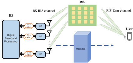
Figure 1: An RIS-aided uplink mmWave MIMO system where the BS is equipped with low-resolution ADCs.

where ${\bf a}_{K_{1}}(z)=[1,e^{-\text{j}2\pi z},\cdots,e^{-\text{j}(K_{1}-1)2\pi z}]^{T}$ is the array steering vector of the vertical direction of the UPA and ${\bf a}_{K_{2}}(x)=[1,e^{-\text{j}2\pi x},\cdots,e^{-\text{j}(K_{2}-1)2\pi x}]^{T}$ is the array steering vector of horizontal direction, and $\otimes$ denotes the Kronecker product. Denote $\vartheta\in[-90^{\circ},90^{\circ})$ and $\varrho\in[-180^{\circ},180^{\circ})$ as the zenith angle and azimuth angle of the UPA, respectively. The spatial frequency pair $(z,x)$ can be denoted by the physical angle pair $(\vartheta,\varrho)$ as

$$z=\frac{d}{\lambda_{\text{c}}}\cos(\vartheta),\quad x=\frac{d}{\lambda_{\text{c}}}\sin(\vartheta)\cos(\varrho),$$ (2)

where $d$ is the element spacing and $\lambda_{\text{c}}$ is the carrier wavelength. In this paper, we assume that $d_{\text{BS}}=d_{\text{RIS}}=\lambda_{\text{c}}/2$. Denote ${\bf H}_{\text{br}}\in\mathbb{C}^{N\times M}$ as the channel from the RIS to the BS, and ${\bf H}_{\text{ru}}\in\mathbb{C}^{M\times Q}$ as the channel from the user to the RIS. From (1) and (2), the channel matrix ${\bf H}_{\text{br}}$ and ${\bf H}_{\text{ru}}$ can be expressed as

$${\bf H}_{\text{br}} =\sum_{l=1}^{L}\alpha_{l}{\bf a}_{N}(\theta_{l},\varphi_{l}){\bf a}^{H}_{M}(\phi_{l},\upsilon_{l}),$$ (3)

$${\bf H}_{\text{ru}} =\sum_{j=1}^{J}{\beta_{j}{\bf a}_{M}(\omega_{j},\psi_{j}){\bf a}^{H}_{Q}(\varpi_{j},\kappa_{j})},$$ (4)

where $L$ and $J$ represent the numbers of propagation paths between the BS and the RIS and between the RIS and the user, respectively. The parameters $\alpha_{l}$ and $\beta_{j}$ denote the complex path gain of the $l$-th path in the RIS-BS channel and that of the $j$-th path in user-RIS channel, respectively. The angles pair $(\theta_{l},\varphi_{l})$ and $(\phi_{l},\upsilon_{l})$ are the AoAs and AoDs of the $l$-th path in the RIS-BS channel, $(\omega_{j},\psi_{j})$ and $(\varpi_{j},\kappa_{j})$ represent the AoAs and AODs of the $j$-th path in the user-RIS channel, respectively. Assume that the RIS phase configuration changes $P$ times during the channel estimation process, and the user sends $T$ time slots of pilot signals in each RIS phase configuration. Then, the received signal at the $p$-th RIS phase configuration ${\bf e}^{p}$ at time slot $t$ and the sum of $T$ time slots are respectively given by

$$\mathbf{y}_{t}^{p} ={{\mathbf{H}}_{\text{br}}}\text{Diag}\left({{\mathbf{e}}^{p}}\right){{\mathbf{H}}_{\text{ru}}}{{\mathbf{s}}_{t}}+\mathbf{w}_{t}^{p},$$ (5)

$${{\mathbf{Y}}^{p}} =\left[\mathbf{y}_{1}^{p},\cdots,\mathbf{y}_{T}^{p}\right]={{\mathbf{H}}_{\text{br}}}\text{Diag}\left({{\mathbf{e}}^{p}}\right){{\mathbf{H}}_{\text{ru}}}\mathbf{S}+{{\mathbf{W}}^{p}},$$ (6)

where ${\bf s}_{t},1\leq t\leq T$ and ${\bf w}^{p}_{t},1\leq t\leq T$ represent the pilot signals transmitted in time slot $t$ and the received noise at the $p$-th RIS phase configuration in time slot $t$, respectively, and ${\bf S}=[{\bf s}_{1},\cdots,{\bf s}_{T}]\in\mathbb{C}^{Q\times T}$, ${\bf W}^{p}=[{\bf w}^{p}_{1},\cdots,{\bf w}^{p}_{T}]\in\mathbb{C}^{N\times T}$.

II-A Cascaded Channel Sparsity Model

By using the virtual angular domain representation, we can approximate the BS-RIS channel ${\bf H}_{\text{br}}$ and the RIS-user channel ${\bf H}_{\text{ru}}$ as

$${\bf H}_{\text{br}} \approx{\bf F}_{N}{\widetilde{\bf H}_{\text{br}}}{\bf F}^{H}_{M},$$

$${\bf H}_{\text{ru}} \approx{\bf F}_{M}{\widetilde{\bf H}_{\text{ru}}}{\bf F}^{H}_{Q},$$ (7)

where ${\widetilde{\bf H}_{\text{br}}}\in\mathbb{C}^{N\times M}$ and ${\widetilde{\bf H}_{\text{ru}}}\in\mathbb{C}^{M\times Q}$ are the angular cascaded channel of the BS-RIS channel and the RIS-user channel, respectively. ${\bf F}_{N}\in\mathbb{C}^{N\times N}$, ${\bf F}_{M}\in\mathbb{C}^{M\times M}$ and ${\bf F}_{Q}\in\mathbb{C}^{Q\times Q}$ are the dictionary matrices. With an $N_{1}\times N_{2}$ UPA at the BS, an $M_{1}\times M_{2}$ UPA at the RIS and a $Q_{1}\times Q_{2}$ UPA at the user, we have

$${\bf H}_{\text{br}} \approx({\bf U}_{N_{1}}\otimes{\bf U}_{N_{2}}){\widetilde{\bf H}_{\text{br}}}({\bf U}^{H}_{M_{1}}\otimes{\bf U}^{H}_{M_{2}}),$$

$${\bf H}_{\text{ru}} \approx({\bf U}_{M_{1}}\otimes{\bf U}_{M_{2}}){\widetilde{\bf H}_{\text{ru}}}({\bf U}^{H}_{Q_{1}}\otimes{\bf U}^{H}_{Q_{2}}),$$ (8)

where ${\bf U}_{n}\in\mathbb{C}^{n\times n}$ denotes the $n$-dimensional discrete Fourier transform (DFT) matrix. In our work, the angles are continuously and uniformly distributed and not necessarily located on grid, which is more practical. By aggregating all signals ${\bf Y}^{p}$ in $P$ RIS phase configuration, the received signal matrix is given by

$$\mathbf{Y} =\left[\text{vec}\left({{\mathbf{Y}}^{1}}\right),\cdots,\text{vec}\left({{\mathbf{Y}}^{P}}\right)\right]+\left[\text{vec}({\bf W}^{1}),\cdots,\text{vec}({\bf W}^{P})\right]$$

$$\overset{a}{=}{{\left({{\mathbf{H}}_{\text{ru}}}\mathbf{S}\right)}^{T}}\diamond{{\mathbf{H}}_{\text{br}}}\mathbf{E}+{\bf W}$$

$$={{{\mathbf{S}^{T}{\mathbf{H}}^{T}_{\text{ru}}}}}\diamond{{\mathbf{H}}_{\text{br}}}\mathbf{E}+{\bf W}$$ (9)

$$={{\left({{\mathbf{F}}_{M}}{{{\mathbf{\widetilde{H}}}}_{\text{ru}}}\mathbf{F}_{Q}^{H}\mathbf{S}\right)}^{T}}\diamond\left({{\mathbf{F}}_{N}}{{{\mathbf{\widetilde{H}}}}_{\text{br}}}\mathbf{F}_{M}^{H}\right)\mathbf{E}+{\bf W}$$

$$\overset{b}{=}\left({{\mathbf{S}}^{T}}\mathbf{F}_{Q}^{*}\otimes{{\mathbf{F}}_{N}}\right)\left(\mathbf{\widetilde{H}}_{\text{ru}}^{T}\otimes{{{\mathbf{\widetilde{H}}}}_{\text{br}}}\right)\left(\mathbf{F}_{M}^{T}\diamond\mathbf{F}_{M}^{H}\right)\mathbf{E}+{\bf W},$$

where ${\bf E}=\left[{\bf e}^{1},\cdots,{\bf e}^{P}\right]$, and the equality $a$ has used the property that $\text{vec}({\bf A}\text{Diag}({\bf b}){\bf C})=({\bf C}^{T}\diamond{\bf A}){\bf b}$ [8], and the operator $\diamond$ denotes the Khatri-Rao product. The equality $b$ is obtained via the property that $({\bf A}\otimes{\bf B})({\bf C}\diamond{\bf D})={\bf AC}\diamond{\bf BD}$. The matrices ${{\mathbf{\widetilde{H}}}}_{\text{br}}$ and ${{\mathbf{\widetilde{H}}}}_{\text{ru}}$ represent the sparse angular domain matrix of the RIS-BS channel and the user-RIS channel, respectively. We aim to estimate the cascaded channel ${\mathbf{H}}^{T}_{\text{ru}}\diamond{\mathbf{H}}_{\text{br}}$. From (II-A), it can be seen that the sparse matrix of the RIS-aided multi-antenna user cascaded channel $\mathbf{\widetilde{H}}_{\text{ru}}^{T}\otimes{{{\mathbf{\widetilde{H}}}}_{\text{br}}}$ is expressed in the form of the Kronecker product, leading to the substantial increase in the number of parameters that needs to be estimated. Fortunately, Proposition 1 in [9] showed that the Khatri-Rao product $\mathbf{F}_{M}^{T}\diamond\mathbf{F}_{M}^{H}$ only contains $M$ distinct rows, which means that the other $M(M-1)$ rows still belong to the first $M$ rows. Based on the above discussions, the cascaded channel matrix can be further compressed, and (II-A) can be equivalently modified as

$${\bf Y}=\underbrace{\left({{\mathbf{S}}^{T}}\mathbf{F}_{Q}^{*}\otimes{{\mathbf{F}}_{N}}\right){\bf\Lambda}\mathbf{F}_{M}^{H}\mathbf{E}}_{\triangleq{\bf Z}}+{\bf W},$$ (10)

where the sparse matrix ${\bf\Lambda}\in\mathbb{C}^{QN\times M}$ is a compressed version of $\left(\mathbf{\widetilde{H}}_{\text{ru}}^{T}\otimes{{{\mathbf{\widetilde{H}}}}_{\text{br}}}\right)\in\mathbb{C}^{QN\times M^{2}}$. More details about the proposition can be found in appendix. Then, the quantization output is given by

$$\widetilde{\bf Y} =\mathcal{Q}\left({\bf Z+W}\right),$$ (11)

where $\mathcal{Q}$ denotes the quantize operation.

II-B ADC Quantization Model

Assume that each quantizer at the BS adopts uniform mid-rise quantization and the variable gain amplifiers are adopted. Denote $\Delta_{\text{Re}}$ and $\Delta_{\text{Im}}$ as the stepsizes of the real part quantizer and the imaginary part quatizer, respectively. Assuming that the input scalar $\xi$ is circularly symmetric, then $\Delta_{\text{Re}}=\Delta_{\text{Im}}=\sqrt{\mathbb{E}\{{|\xi|^{2}}/{2}\}}\Delta$. The coefficient $\Delta$ can be found in [10]. For a $B$-bit quantizer, the analog input magnitude is divided into $2^{B}-1$ thresholds, which is denoted as $h_{1},h_{2},\cdots,h_{2^{B}-1}$, where $h_{b}=(-2^{B-1}+b)\Delta_{\text{Re}},1\leq b\leq 2^{B}$. Once the input signal falls in the interval $[h_{b-1},h_{b})$, the output is set to $h_{b}-\frac{\Delta_{\text{Re}}}{2}$.

III Channel Estimation Algorithm

In this section, we aim to estimate the cascaded channel based on the quantized output $\widetilde{\bf Y}$ and the predetermined training matrix ${\bf E}$. The VAMP-based channel estimation strategy for a multi-antenna user is first described. Then, we propose the corresponding fast computation implementation for the channel estimation algorithm. Finally, the computational complexity of the fast implementation method is analyzed.

III-A Problem Formulation

Based on the above discussions, to estimate the cascaded channel, we only need to estimate the sparse matrix $\bf\Lambda$. Defining $\widetilde{\bf y}\triangleq\text{vec}\left(\widetilde{\bf Y}\right)$, ${\bf x}\triangleq\text{vec}\left({\mathbf{{\Lambda}}}\right)$ and ${\bf w}\triangleq\text{vec}\left({\bf W}\right)$, (11) can be vectorized as

$$\widetilde{\bf y}=\mathcal{Q}\left(\underbrace{{{\left({{\mathbf{F}}^{H}_{M}}\mathbf{E}\right)}^{T}}\otimes\left({\bf S}^{T}\mathbf{F}_{Q}^{*}\otimes{{\mathbf{F}}_{N}}\right)}_{\triangleq{\bf A}}{\bf x}+{\bf w}\right).$$ (12)

From (12), the cascaded channel estimation can be formulated as the following problem: estimate the sparse vector ${\bf{x}}\in\mathbb{C}^{NMQ}$ from the observation $\tilde{\bf y}\in\mathbb{C}^{PTN}$ based on the known linear transform ${\bf{A}}\in\mathbb{C}^{PTN\times NMQ}$.

III-B VAMP Algorithm

According to (12), the cascaded channel estimation can be formulated as a noisy quantized CS problem. To reconstruct the noiseless signal $\bf z$ and the sparse vector $\bf x$ from $\tilde{\bf y}$, we introduce the efficient VAMP algorithm [11] to implement the Bayesian optimal estimators. Assume that $\bf z$ is produced by a linear transform ${\bf z}={\bf Ax}$ by a sparse vector ${\bf x}$ with i.i.d elements and a known matrix ${\bf A}$. Based on the observation $\tilde{\bf y}=\mathcal{Q}({\bf Ax}+{\bf w})$ and the likelihood $p(\tilde{\bf y}|{\bf z})=\prod_{i}{p_{Y|Z}(y_{i}|z_{i})}$, the VAMP algorithm can approach nearly minimum mean square error (MMSE) estimation of ${\bf x}$ by alternatively calculating the scalar estimation and linear MMSE (LMMSE) estimation iteratively.

Without loss of generality, suppose the elements $x_{i},\forall i$ follow the Bernoulli Gaussian-mixtrue (GM) with parameters $\bf q$ as

$$p_{X}\left(x_{i};{\bf q}\right)=\lambda_{0}\delta\left(x_{i}\right)+\sum_{i}\lambda_{i}\mathcal{CN}\left(x_{i};\mu_{i},\rho_{i}\right),\forall i,$$ (13)

where ${\bf q}\triangleq\{\{\lambda_{i}\},\{\mu_{i}\},\{\rho_{i}\}\},\forall i$ denotes the prior parameters set and $\lambda_{0}=\text{Prob}\{x=0\}$, and $\{\lambda_{i}\}$, $\{\mu_{i}\}$ and $\{\rho_{i}\}$ are the weights of the distributions, means and variances of the Gaussian mixture, respectively.

Algorithm 1 gives the details of the VAMP algorithm, where $T_{\text{max}}$ is the number of maximum iteration time and it is set to 50 in our simulation. Steps 4 and 5 calculate the posterior mean and variance of $x$ based on the pseudo-prior $p_{X}(x)$ and the likelihood $p(x|r_{1})$, where the quality ${\bf r}_{1}$ is the additive white Gaussian noise (AWGN) corrupted version of ${\bf x}$, i.e. ${\bf r}_{k}={\bf x}+\mathcal{CN}({\bf 0},\nu^{x}{\bf I})$, and the variance $\nu^{x}$ is computed iteratively. The posterior probability $p(x_{1m}|r_{1m})$ is given by

$$p_{X|R}\left(x_{m}|\hat{r}_{m};\nu_{m}^{r},{\bf q}\right)\triangleq\frac{p_{X}\left(x_{m};{\bf q}\right)\mathcal{CN}\left(x_{m};\hat{r}_{m},\nu_{m}^{r}\right)}{\int_{x}p_{X}(x;{\bf q})\mathcal{CN}\left(x;\hat{r}_{m},\nu_{m}^{r}\right)}.$$ (14)

Step 6 updates the quality ${\bf r}_{2}$ by using an “Osanger” term $\alpha_{k}{\bf r}_{1}$. Steps 7 and 8 calculate the posterior mean and variance of $\bf z$ from the quantization output $\tilde{\bf y}=\mathcal{Q}({\bf z}+{\bf w})$. Assume that the $n$-th element of ${\bf z}$ follows the complex Gaussian distribution of $p(z_{n})=\mathcal{CN}(z_{n};\hat{p_{n}},\nu_{p})$, then the posterior can be computed as

$$p_{Z|Y,P}\left(z_{n}|\tilde{y}_{n};\hat{p}_{n},\nu_{p}\right)\triangleq\frac{p_{Y\mid Z}\left(\tilde{y}_{n}|z_{n}\right)\mathcal{CN}\left(z_{n};\hat{p}_{n},\nu_{p}\right)}{\int_{z}p_{Y\mid Z}\left(\tilde{y}_{n}|z\right)\mathcal{CN}\left(z;\hat{p}_{n},\nu_{p}\right)}.$$ (15)

The details about the derivations of posterior function $p(z|\tilde{y})$ and the posterior mean $\hat{z}$ and variance $\nu^{z}$ can be found in [4]. Then, based on the pseudo-prior of $z$ and $x$, steps 10 to 14 calculate the LMMSE estimation of ${\bf x}$ and ${\bf z}$ jointly.

Algorithm 1 VAMP-based Cascaded Channel Estimation Algorithm

0:  $\widetilde{\bf Y}$, ${\bf p}_{1}$, ${\bf r}_{1}$, $p(\widetilde{\bf Y}|{\bf Z})$ and ${\bf q}$

0:  $\widehat{\bf x}$

1:  Initialize: $\hat{s}=0,\hat{x}_{1}=\int_{x}xp_{X}(x),\forall i,$$\nu^{x}_{m}=\int_{x}\left|x-\hat{x}_{m}(1)\right|^{2}p_{X}(x)$

2:  for $t=1,\cdots,T_{\text{max}}$ do

3:     $\widehat{x}_{1i}\leftarrow\mathbb{E}_{X\mid R}\left[x_{i}\mid r_{1i};\nu^{x}_{1},{\bf q}\right],\quad\forall i$

4:     $\alpha_{1}\leftarrow\frac{1}{\nu^{x}_{1}NMQ}\sum_{i=1}^{NMQ}\operatorname{Var}_{X\mid R}\left[x_{i}\mid r_{1i};\nu^{x}_{1},{\bf q}\right]$

5:     $\mathbf{r}_{2}\leftarrow\left(\widehat{\mathbf{x}}_{1}-\alpha_{1}\mathbf{r}_{1}\right)/\left(1-\alpha_{1}\right),\ \ \nu^{x}_{2}\leftarrow\nu^{x}_{1}\alpha_{1}/\left(1-\alpha_{1}\right)$

6:     $\widehat{z}_{1i}\leftarrow\mathbb{E}_{Z\mid Y,P}\left[z_{i}\mid y_{i},p_{1i};\nu^{p}\right],\ \ \forall i$

7:     $\beta_{1}\leftarrow\frac{1}{\nu^{p}_{1}PNQ}\sum_{i=1}^{PNQ}\operatorname{Var}_{Z\mid Y,P}\left[z_{i}\mid y_{i},p_{1i};\nu^{p}_{1}\right]$

8:     $\mathbf{p}_{2}\leftarrow\left(\widehat{\mathbf{z}}_{1}-\beta_{1}\mathbf{p}_{1}\right)/\left(1-\beta_{1}\right),\quad\nu^{p}_{2}\leftarrow\nu^{p}_{1}\beta_{1}/\left(1-\beta_{1}\right)$

9:     $\widehat{\mathbf{x}}_{2}\leftarrow\mathbf{V}_{A}\left({\bf S}^{H}_{A}{\bf S}_{A}\nu^{x}_{2}/\nu^{p}_{2}+\mathbf{I}\right)^{-1}\times$ $\left({\bf V}_{A}{\bf A}^{H}\mathbf{p}_{2}\nu^{x}_{2}/\nu^{p}_{2}\right.\left.+\mathbf{V}_{A}^{H}\mathbf{r}_{2}\right)$, where ${\bf V}_{A}$ and ${\bf S}^{H}_{A}{\bf S}_{A}$ are defined in (III-C), and each terms of $\widehat{\bf x}_{2}$ can be calculated via FFT similar to step 13

10:     $\alpha_{2}\leftarrow\frac{1}{NMQ}\sum_{n=1}^{NMQ}\nu^{p}_{2}/\left(s_{n}^{2}\nu^{x}_{2}+\nu^{p}_{2}\right)$

11:     $\mathbf{r}_{1}\leftarrow\left(\widehat{\mathbf{x}}_{2}-\alpha_{2}\mathbf{r}_{2}\right)/\left(1-\alpha_{2}\right),\ \ \nu^{x}_{1}\leftarrow\nu^{x}_{2}\alpha_{2}/\left(1-\alpha_{2}\right)$

12:     Calculate $\widehat{\mathbf{z}}_{2}\leftarrow\mathbf{A}\widehat{\mathbf{x}}_{2}$ by using FFT and (A1)-(A4)

13:     $\beta_{2}\leftarrow\left(1-\alpha_{2}\right)PT/M$

14:     $\mathbf{p}_{1}\leftarrow\left(\widehat{\mathbf{z}}_{2}-\beta_{2}\mathbf{p}_{2}\right)/\left(1-\beta_{2}\right),\ \ \nu^{p}_{1}\leftarrow\nu^{p}_{2}\beta_{2}/\left(1-\beta_{2}\right)$

15:  end for

III-C Fast Computation Implementation

To tackle the information loss caused by few-bit quantization, the training length needs to reach hundreds to provide more measurements to estimate the channel. For the VAMP algorithm, most of the complexity comes from calculating the matrix-vector product ${\bf A}\widehat{\bf x}_{2}$ and ${\bf V}^{H}_{A}{\bf r}_{2}$ in each iteration, where , whose computational complexity is $\mathcal{O}(PN^{2}M)$ and $\mathcal{O}(N^{2}M^{2})$, respectively.

To lower the computational complexity, a fast implementation method to compute ${\bf A}\widehat{\bf x}$ is proposed based on FFT. The received signal in (10) can be further rewritten as

$${\bf Y}=\left({{\mathbf{S}}^{T}}\mathbf{F}_{Q}^{*}\otimes{{\mathbf{F}}_{N}}\right)\left(\mathbf{E}^{T}\mathbf{F}_{M}^{\ast}{\bf\Lambda}^{T}\right)^{T}+{\bf W}.$$ (16)

We can respectively obtain $\mathbf{F}_{M}^{\ast}{\bf\Lambda}^{T}$ by performing 2-D inverse-FFT. Then, left multiple ${\bf E}^{T}$ by using fast convolution and obtain $\mathbf{E}^{T}\mathbf{F}_{M}^{\ast}{\bf\Lambda}^{T}$.

The computation of $\left({{\mathbf{S}}^{T}}\mathbf{F}_{Q}^{*}\otimes{{\mathbf{F}}_{N}}\right)\left(\mathbf{E}^{T}\mathbf{F}_{M}^{\ast}{\bf\Lambda}^{T}\right)^{T}$ can be performed as follows. Denote ${\bf X}\triangleq\left(\mathbf{E}^{T}\mathbf{F}_{M}^{\ast}{\bf\Lambda}^{T}\right)^{T}\in\mathbb{C}^{NQ\times P}$ and reshape $\bf X$ as a three way tensor ${\mathcal{X}}\in\mathbb{C}^{N\times Q\times P}$. Then, the multiplication $\left({{\mathbf{S}}^{T}}\mathbf{F}_{Q}^{*}\otimes{{\mathbf{F}}_{N}}\right){\bf X}$ can be rewritten as

$$\left({{\mathbf{S}}^{T}}\mathbf{F}_{Q}^{*}\otimes{{\mathbf{F}}_{N}}\right){\bf X}=\left[\text{vec}\left({\bf F}_{N}{\mathcal{X}}(:,:,1){\bf F}^{\ast}_{Q}{\bf S}\right),\cdots,\text{vec}\left({\bf F}_{N}{\mathcal{X}}(:,:,P){\bf F}^{\ast}_{Q}{\bf S}\right)\right].$$ (17)

Substituting ${{\mathbf{F}}_{N}}={{\mathbf{U}}_{{{N}_{1}}}}\otimes{{\mathbf{U}}_{{{N}_{2}}}}$ and ${{\mathbf{F}}_{Q}}={{\mathbf{U}}_{{{Q}_{1}}}}\otimes{{\mathbf{U}}_{{{Q}_{2}}}}$ into (17), we have

$${{\mathbf{F}}_{N}}{\mathcal{X}}\left(:,:,p\right)\mathbf{F}_{Q}^{*}{\bf S} =\left({{\mathbf{U}}_{{{N}_{1}}}}\otimes{{\mathbf{U}}_{{{N}_{2}}}}\right){\mathcal{X}}\left(:,:,p\right)\left(\mathbf{U}_{{{Q}_{1}}}^{*}\otimes\mathbf{U}_{{{Q}_{2}}}^{*}\right){\bf S}$$

$$=\left({{\mathbf{U}}_{{{N}_{1}}}}\otimes{{\mathbf{U}}_{{{N}_{2}}}}\right){{\left({\bf S}^{T}\left(\mathbf{U}_{{{Q}_{1}}}^{*}\otimes\mathbf{U}_{{{Q}_{2}}}^{*}\right)({{{\mathcal{X}}}}\left(:,:,p\right))^{T}\right)}^{T}},\forall p.$$ (18)

Note that the $i$-th vector of the multiplication $\left(\mathbf{U}_{{{X}_{1}}}\otimes\mathbf{U}_{{{X}_{2}}}\right){\bf X}$ can be denoted as $\left(\mathbf{U}_{{{X}_{1}}}\otimes\mathbf{U}_{{{X}_{2}}}\right){\bf X}_{:,i}={\text{vec}}(\mathbf{U}_{{{X}_{2}}}{\bf X}_{i}\mathbf{U}_{{{X}_{1}}}^{T})$, where ${\bf X}_{i}=\text{unvec}({\bf X}_{:,i})$, and thus we can calculate each vector of the multiplication $\left(\mathbf{U}_{{{X}_{1}}}\otimes\mathbf{U}_{{{X}_{2}}}\right){\bf X}$ by using 2-D FFT. Similarly, we can calculate each vector of the multiplication $\left(\mathbf{U}_{{{X}_{1}}}^{*}\otimes\mathbf{U}_{{{X}_{2}}}^{*}\right){\bf X}$ by using 2-D IFFT. Based on the above discussions, the steps for fast computation of ${{\mathbf{F}}_{N}}{\mathcal{X}}\left(:,:,p\right)\mathbf{F}_{Q}^{*}{\bf S}$ are as follows:

(A1) Permute ${\mathcal{X}}\in\mathbb{C}^{N\times Q\times P}$ to ${\mathcal{X}}_{1}\in\mathbb{C}^{Q\times N\times P}$, and reshape it to ${\mathcal{X}}_{2}\in\mathbb{C}^{Q_{1}\times Q_{2}\times NP}$.

(A2) Do 2-D inverse-FFT for each slice ${\mathcal{X}}_{2}(:,:,i)$, and then reshape to ${\mathcal{X}}_{3}\in\mathbb{C}^{Q\times N\times P}$.

(A3) Calculate ${\bf S}^{T}{\mathcal{X}}_{3}(:,:,i)$, and permute to ${\mathcal{X}}_{4}\in\mathbb{C}^{N\times Q\times P}$, then reshape it to ${\mathcal{X}}_{5}\in\mathbb{C}^{N_{1}\times N_{2}\times QP}$.

(A4) Do 2-D FFT for each slice ${\mathcal{X}}_{5}(:,:,i)$, and then reshape to $\widetilde{\bf X}\in\mathbb{C}^{NQ\times P}$, and we obtain $\widetilde{\bf X}=\left({{\mathbf{S}}^{T}}\mathbf{F}_{Q}^{*}\otimes{{\mathbf{F}}_{N}}\right){\bf X}$.

The computation of the multiplication ${\bf V}^{H}_{A}{\bf r}$ follows a similar procedure. Specifically, let ${\bf S}={\bf I}_{Q}$ and we have

$${\bf A}^{H}{\bf A} =\left({\bf F}^{T}_{M}{\bf E}^{\ast}{\bf E}^{T}{\bf F}^{\ast}_{M}\right)\otimes NQ{\bf I}_{NQ}$$

$$=NMQ\left(\frac{1}{\sqrt{M}}{\bf F}^{T}_{M}{\bf U}_{E}\otimes{\bf I}_{NQ}\right)\left({\bf\Lambda}_{E}\otimes{\bf I}_{NQ}\right)\left(\frac{1}{\sqrt{M}}{\bf U}^{H}_{E}{\bf F}^{\ast}_{M}\otimes{\bf I}_{NQ}\right)$$

$$={\bf V}_{A}{\bf S}_{A}^{H}{\bf S}_{A}{\bf V}^{H}_{A},$$ (19)

where ${\bf V}_{A}\triangleq\left(\frac{1}{\sqrt{M}}{\bf F}^{T}_{M}{\bf U}_{E}\otimes{\bf I}_{NQ}\right)$ and ${\bf U}_{E}$ and ${\bf\Lambda}_{E}$ are the eigen vectors and the eigenvalues of ${\bf E}^{\ast}{\bf E}^{T}$, respectively. Thus, the multiplication ${\bf V}^{H}_{A}{\bf r}$ can be also fast computed by using FFT similarly.

III-D Complexity Analysis

For the VAMP algorithm, most of the computational complexity is introduced by the matrix multiplications ${\bf A}\widehat{\bf x}$. For a general measurement matrix $\bf A$, it needs the complexity of $\mathcal{O}(PMN^{2}Q^{2})$. In our proposed algorithm, the fast computations of ${\bf E}^{T}{\bf F}^{\ast}_{M}{\bf\Lambda}^{T}$ need $NQ$ times of $P$ points FFT and IFFT, and $NQ$ times of $P$ points Hadamard products, the corresponding complexity is $\mathcal{O}(2NPQ\log P)$. Furthermore, the steps for fast computation of ${\bf F}_{N}{\mathcal{X}}(:,:,p){\bf F}^{\ast}_{Q}{\bf S}$ needs $NP$ times 2-D IFFT, $P$ times of matrix multiplication ${\bf S}^{T}{\mathcal{X}}(:,:,i)$ and $QP$ times of 2-D FFT. However, the signal matrix ${\bf S}$ can be simply substituted by ${\bf I}_{Q}$ or $Q$ points DFT matrix, and the matrix multiplication can be avoided, and the corresponding complexity is $\mathcal{O}(NPQ\log NQ)$. Hence, the total computational complexity for the VAMP algorithm is $T_{\text{max}}\mathcal{O}(2QPN\log QPN)$.

IV Simulation Results

In this section, the simulation results are presented to show the efficiency of the proposed method. Both the BS and the RIS are equipped with a UPA. The antenna spacing is half-wavelength. The SNR is defined as SNR $\triangleq\frac{\mathbb{E}\left[\|{\bf Z}\|^{2}_{F}\right]}{\mathbb{E}\left\{\|{\bf W}\|^{2}_{F}\right\}}$, where $\mathbb{E}\left\{\|{\bf Z}\|^{2}_{F}\right\}=\mathbb{E}\left\{\|({\bf S}^{T}{\bf H}^{T}_{\text{ru}}\diamond{\bf H}_{\text{br}}){\bf E}\|^{2}_{F}\right\}$. The scales of the UPAs employed at the BS and the RIS are $N_{1}=N_{2}=8$ and $M_{1}=M_{2}=8$, respectively. The multi-antenna user is equipped with a $2\times 2$ UPA, i.e., $Q_{1}=Q_{2}=2$. The set of angular parameters are generated from uniform distribution. The normalized mean square error (NMSE) is defined as NMSE$({\bf G})\triangleq\mathbb{E}\left\{\frac{\|{\bf G}-\widehat{\bf G}\|^{2}_{F}}{\|{\bf G}\|^{2}_{F}}\right\}$, where ${\bf G}\triangleq{\bf H}^{T}_{\text{ru}}\diamond{\bf H}_{\text{br}}$, and $\widehat{\bf G}$ is the estimated cascaded channel. The LS algorithm, the Bussgang theorem based LMMSE (BLM) algorithm, the quantized iterative hard thresholding (QIHT) algorithm [12], the basis pursuit denosing (BPDN) algorithm [13] are chosen as the benchmark algorithms.

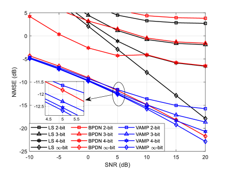
Figure 2: NMSE versus SNR, $K=4$.

Fig. 2 illustrates the NMSE performance versus the SNR, where the number of users $K=4$, and the training length is set to $PT=512$. Compared with the LS algorithm and the BPDN algorithm, the Bayes inference based channel estimation method is more accurate. In addition, for low and medium SNR ($\leq$10 dB), the gap of NMSE between the few-bit ADCs (2-4 bits) and infinite-bit ADCs is less than 3 dB, which shows the applicability of few-bit ADCs in practice.

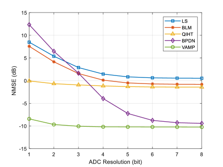
Figure 3: NMSE versus Bit number.

Fig. 3 shows the NMSE performance versus the number of bits for the multi-antenna user scenario, where SNR $=$ 0 dB. As shown in Fig. 3, the proposed VAMP-based algorithms outperform the other benchmark algorithms. The BPDN algorithm performs similarly to VAMP when the ADC precision reaches to 6, 7, 8 and infinite bit, but performs worse for few-bit ADCs.

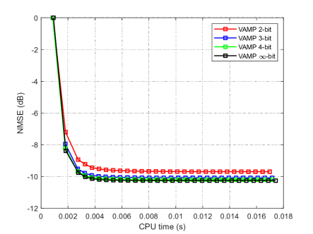
Figure 4: NMSE versus CPU time.

In Fig. 4, the NMSE versus the runtime by varying the number of iterations for the VAMP algorithm under the multi-antenna user scenario is demonstrated, where SNR $=$ 0 dB. For the 2, 3 and 4-bit quantization, the VAMP based cascaded channel estimation algorithm only needs less than 10 iterations to converge and the runtimes are less than 0.02s due to the proposed FFT based fast implements, which demonstrates the low computational complexity for the VAMP based cascaded channel estimation algorithm.

V Conclusion

In this paper, we studied the cascaded channel estimation for an RIS-aided mmWave massive MIMO system, where the BS is equipped with few-bit ADCs and the BS, the RIS and the user are employed with UPAs. Considering the sparse property of the mmWave cascaded channel, we formulated the corresponding CS problem. To tackle with the information loss caused by coarse quantization, we adopted the Bayesian inference and VAMP algorithm to recovery the received signals and the sparse angular domain cascaded channel iteratively. The corresponding fast computation algorithm was derived to lower the complexity. The proposed strategy outperforms the other benchmark algorithms. Furthermore, the performance gap between low-precision ADCs and ideal infinite precision ADCs is acceptable for low and medium SNR, which implied that the low-precision ADCs is applicable for the low and medium SNR scenario.

Appendix A Proof of Proposition in [9]

We provide a detailed proof that ${\bf Y}=\left({{\mathbf{S}}^{T}}\mathbf{F}_{Q}^{*}\otimes{{\mathbf{F}}_{N}}\right)\left(\mathbf{\widetilde{H}}_{\text{ru}}^{T}\otimes{{{\mathbf{\widetilde{H}}}}_{\text{br}}}\right)\left(\mathbf{F}_{M}^{T}\diamond\mathbf{F}_{M}^{H}\right)\mathbf{E}+{\bf W}$ can be compressed as ${\bf Y}={\left({{\mathbf{S}}^{T}}\mathbf{F}_{Q}^{*}\otimes{{\mathbf{F}}_{N}}\right){\bf\Lambda}\mathbf{F}_{M}^{H}\mathbf{E}}+{\bf W}$. Denotes $\mathbf{F}_{M}=\left[\mathbf{f}_{1},\cdots,\mathbf{f}_{M}\right]$, then the Khatri-Rao product $\mathbf{F}_{M}^{T}\diamond\mathbf{F}_{M}^{H}$ can be written as

$$\left(\mathbf{F}_{M}^{T}\diamond\mathbf{F}_{M}^{H}\right)=\left[\begin{array}[]{l}\mathbf{F}_{M}^{H}\mathrm{Diag}\left(\mathbf{f}_{1}\right)\\ \vdots\\ \mathbf{F}_{M}^{H}\mathrm{Diag}\left(\mathbf{f}_{M}\right)\\ \end{array}\right].$$ (20)

Since $\mathbf{F}_{M}=\mathbf{U}_{M_{1}}\otimes\mathbf{U}_{M_{2}}$, we have

$$\mathbf{F}_{M}^{H}\mathrm{Diag}\left(\mathbf{f}_{m}\right) =\left(\mathbf{U}_{M_{1}}^{H}\otimes\mathbf{U}_{M_{2}}^{H}\right)\mathrm{Diag}\left(\mathbf{f}_{m}\right)$$

$$=\left(\mathbf{U}_{M_{1}}^{H}\otimes\mathbf{U}_{M_{2}}^{H}\right)\mathrm{Diag}\left(\left[\begin{array}[]{c}u_{m_{1},1}\mathbf{u}_{M_{2}}\left(:,m_{2}\right)\\ \vdots\\ u_{m_{1},M_{1}}\mathbf{u}_{M_{2}}\left(:,m_{2}\right)\\ \end{array}\right]\right)$$ (24)

$$=\left(\begin{matrix}u_{1,1}^{\ast}u_{m_{1},1}\mathbf{U}_{M_{2}}^{H}\mathrm{Diag}\left(\mathbf{u}_{M_{2}}\left(:,m_{2}\right)\right)&\cdots&u_{M_{1},1}^{\ast}u_{m_{1},M_{1}}\mathbf{U}_{M_{2}}^{H}\mathrm{Diag}\left(\mathbf{u}_{M_{2}}\left(:,m_{2}\right)\right)\\ \vdots&\ddots&\vdots\\ u_{1,M_{1}}^{\ast}u_{m_{1},1}\mathbf{U}_{M_{2}}^{H}\mathrm{Diag}\left(\mathbf{u}_{M_{2}}\left(:,m_{2}\right)\right)&\cdots&u_{M_{1},M_{1}}^{\ast}u_{m_{1},M_{1}}\mathbf{U}_{M_{2}}^{H}\mathrm{Diag}\left(\mathbf{u}_{M_{2}}\left(:,m_{2}\right)\right)\\ \end{matrix}\right),$$ (25)

where $m_{1}$ and $m_{2}$ are the corresponding entry and the column index of the $m$-th column of ${\bf F}_{M}=\mathbf{U}_{M_{1}}\otimes\mathbf{U}_{M_{2}}$, respectively. Note that the DFT matrix has the following property

$$\mathbf{U}_{M_{2}}^{H}\mathrm{Diag}\left(\mathbf{u}_{M_{2}}\left(:,m_{2}\right)\right)=\mathbf{\Pi}_{m_{2}}\mathbf{U}_{M_{2}}^{H}.$$ (26)

where the permutation matrix $\mathbf{\Pi}_{m_{2}}$ is associated with the index $m_{2}$. The reason of this property is that any two columns $\mathbf{u}_{M_{2}}\left(:,x_{1}\right)$ and $\mathbf{u}_{M_{2}}\left(:,x_{2}\right)$ from DFT matrix $\mathbf{U}_{M_{2}}$, the hadamard product of the two columns $\mathbf{u}_{M_{2}}\left(:,x_{1}\right)\odot\mathbf{u}_{M_{2}}\left(:,x_{2}\right)$ still belongs to the columns of the DFT matrix. Hence, we can prove that

$$\left(\begin{matrix}u_{1,1}^{\ast}u_{m_{1},1}\mathbf{U}_{M_{2}}^{H}\mathrm{Diag}\left(\mathbf{u}_{M_{2}}\left(:,m_{2}\right)\right)&\cdots&u_{M_{1},1}^{\ast}u_{m_{1},M_{1}}\mathbf{U}_{M_{2}}^{H}\mathrm{Diag}\left(\mathbf{u}_{M_{2}}\left(:,m_{2}\right)\right)\\ \vdots&\ddots&\vdots\\ u_{1,M_{1}}^{\ast}u_{m_{1},1}\mathbf{U}_{M_{2}}^{H}\mathrm{Diag}\left(\mathbf{u}_{M_{2}}\left(:,m_{2}\right)\right)&\cdots&u_{M_{1},M_{1}}^{\ast}u_{m_{1},M_{1}}\mathbf{U}_{M_{2}}^{H}\mathrm{Diag}\left(\mathbf{u}_{M_{2}}\left(:,m_{2}\right)\right)\\ \end{matrix}\right)$$

$$\qquad=\left(\begin{matrix}u_{1,1}^{\ast}u_{m_{1},1}\mathbf{\Pi}_{m_{2}}\mathbf{U}_{M_{2}}^{H}&\cdots&u_{M_{1},1}^{\ast}u_{m_{1},M_{1}}\mathbf{\Pi}_{m_{2}}\mathbf{U}_{M_{2}}^{H}\\ \vdots&\ddots&\vdots\\ u_{1,M_{1}}^{\ast}u_{m_{1},1}\mathbf{\Pi}_{m_{2}}\mathbf{U}_{M_{2}}^{H}&\cdots&u_{M_{1},M_{1}}^{\ast}u_{m_{1},M_{1}}\mathbf{\Pi}_{m_{2}}\mathbf{U}_{M_{2}}^{H}\\ \end{matrix}\right)$$

$$\qquad=\left(\begin{matrix}u_{m_{1},1}\mathbf{\Pi}_{m_{2}}\mathbf{U}_{M_{2}}^{H}&\cdots&u_{m_{1},M_{1}}\mathbf{\Pi}_{m_{2}}\mathbf{U}_{M_{2}}^{H}\\ \vdots&\ddots&\vdots\\ u_{m_{1}+1,1}\mathbf{\Pi}_{m_{2}}\mathbf{U}_{M_{2}}^{H}&\cdots&u_{m_{1}+1,M_{1}}\mathbf{\Pi}_{m_{2}}\mathbf{U}_{M_{2}}^{H}\\ \end{matrix}\right)$$

$$\qquad=\left(\mathbf{\Pi}_{m_{1}}\mathbf{U}_{M_{1}}^{H}\right)\otimes\left(\mathbf{\Pi}_{m_{2}}\mathbf{U}_{M_{2}}^{H}\right).$$ (27)

Analogously, it can be derived that the last $M(M-1)$ rows are the permutation version of the first $M$ rows and they still belongs to the first $M$ rows. Based on the above discussion, we can obtain that ${\bf\Lambda}$ is the compressed version of $\left(\mathbf{\widetilde{H}}_{\text{ru}}^{T}\otimes{{{\mathbf{\widetilde{H}}}}_{\text{br}}}\right)$

$$\mathbf{\Lambda}\left(:,i\right)=\sum_{n\in\mathcal{S}_{i}}{\left(\widetilde{\mathbf{H}}_{\mathrm{ru}}^{T}\otimes\widetilde{\mathbf{H}}_{\mathrm{br}}\right)_{:,n}},$$ (28)

where $\mathbf{\Lambda}\left(:,i\right)$ denotes the $i$-th column of $\bf\Lambda$ and $\mathcal{S}_{i}$ denotes the set of indices associated with those rows in $\left(\mathbf{F}_{M}^{T}\diamond\mathbf{F}_{M}^{H}\right)$ that are identical to the $i$-th row of $\left(\mathbf{F}_{M}^{T}\diamond\mathbf{F}_{M}^{H}\right)$ [9].

References

• [1] S. A. Busari, K. M. S. Huq, S. Mumtaz, L. Dai, and J. Rodriguez, “Millimeter-wave massive MIMO communication for future wireless systems: A survey,” IEEE Commun. Surveys Tuts., vol. 20, no. 2, pp. 836–869, Dec. 2017.
• [2] S. Mumtaz, J. Rodriguez, and L. Dai, MmWave Massive MIMO: A Paradigm for 5G.   Academic Press, 2016.
• [3] B. Le, T. W. Rondeau, J. H. Reed, and C. W. Bostian, “Analog-to-digital converters,” IEEE Signal Process. Mag., vol. 22, no. 6, pp. 69–77, Nov. 2005.
• [4] C.-K. Wen, C.-J. Wang, S. Jin, K.-K. Wong, and P. Ting, “Bayes-optimal joint channel-and-data estimation for massive MIMO with low-precision ADCs,” IEEE Trans. Signal Process., vol. 64, no. 10, pp. 2541–2556, May 2016.
• [5] K. Zhi, C. Pan, H. Ren, and K. Wang, “Uplink achievable rate of intelligent reflecting surface-aided millimeter-wave communications with low-resolution ADC and phase noise,” IEEE Wireless Commun. Lett., vol. 10, no. 3, pp. 654–658, Mar 2021.
• [6] L. Fan, S. Jin, C.-K. Wen, and H. Zhang, “Uplink achievable rate for massive MIMO systems with low-resolution ADC,” IEEE Commun. Lett., vol. 19, no. 12, pp. 2186–2189, Dec. 2015.
• [7] Z. Peng, G. Zhou, C. Pan, H. Ren, A. L. Swindlehurst, P. Popovski, and G. Wu, “Channel estimation for RIS-aided multi-user mmwave systems with uniform planar arrays,” IEEE Trans. Commun., vol. 70, no. 12, pp. 8105–8122, Dec. 2022.
• [8] N. D. Sidiropoulos, L. De Lathauwer, X. Fu, K. Huang, E. E. Papalexakis, and C. Faloutsos, “Tensor decomposition for signal processing and machine learning,” IEEE Trans. Signal Process., vol. 65, no. 13, pp. 3551–3582, Apr. 2017.
• [9] P. Wang, J. Fang, H. Duan, and H. Li, “Compressed channel estimation for intelligent reflecting surface-assisted millimeter wave systems,” IEEE Signal Process. Lett., vol. 27, pp. 905–909, May 2020.
• [10] J. Mo, P. Schniter, and R. W. Heath, “Channel estimation in broadband millimeter wave MIMO systems with few-bit ADCs,” IEEE Trans. Signal Process., vol. 66, no. 5, pp. 1141–1154, Mar 2018.
• [11] S. Rangan, P. Schniter, and A. K. Fletcher, “Vector approximate message passing,” IEEE Trans. Inf. Theory, vol. 65, no. 10, pp. 6664–6684, Oct. 2019.
• [12] L. Jacques, K. Degraux, and C. De Vleeschouwer, “Quantized iterative hard thresholding: Bridging 1-bit and high-resolution quantized compressed sensing.” [Online]. Available: https://arxiv.org/abs/1305.1786
• [13] E. Van Den Berg and M. P. Friedlander, “Probing the pareto frontier for basis pursuit solutions,” SIAM J. Sci. Comput., vol. 31, no. 2, pp. 890–912, May 2009.