Sequential Monte-Carlo testing by betting

Abstract

In a Monte-Carlo test, the observed dataset is fixed, and several resampled or permuted versions of the dataset are generated in order to test a null hypothesis that the original dataset is exchangeable with the resampled/permuted ones. Sequential Monte-Carlo tests aim to save computational resources by generating these additional datasets sequentially one by one, and potentially stopping early. While earlier tests yield valid inference at a particular prespecified stopping rule, our work develops a new anytime-valid Monte-Carlo test that can be continuously monitored, yielding a p-value or e-value at any stopping time possibly not specified in advance. Despite the added flexibility, it significantly outperforms the well-known method by Besag and Clifford, stopping earlier under both the null and the alternative without compromising power. The core technical advance is the development of new test martingales (nonnegative martingales with initial value one) for testing exchangeability against a very particular alternative. These test martingales are constructed using new and simple betting strategies that smartly bet on the relative ranks of generated test statistics. The betting strategies are guided by the derivation of a simple log-optimal betting strategy, have closed form expressions for the wealth process, provable guarantees on resampling risk, and display excellent power in practice.

1 Introduction

Suppose we have some data $X_{0}$, from which we calculate a test statistic $T(X_{0})$. Suppose further that we have the ability to generate additional data $X_{1},X_{2},\dots,X_{B}$ and calculate test statistics $T(X_{1}),T(X_{2}),\dots,T(X_{B})$. Denoting $Y_{i}=T(X_{i})$, assume further that $Y_{1},\dots,Y_{B}$ are always exchangeable conditional on $Y_{0}$. Suppose that we are trying to test the null hypothesis

$$H_{0}:Y_{0},Y_{1},\dots Y_{B}\text{ are exchangeable.}$$

This type of null appears in permutation tests (for example, when performing two-sample or independence testing), but also in many other settings. While we focus on permutation tests for concreteness, the reader may safely substitute “Monte-Carlo” for “permutation” in all occurrences. In particular the methods also apply without alteration to conditional randomization tests frequently encountered in causal inference, and Monte-Carlo tests of group invariance for any other group actions beyond permutations (such as sign symmetry or rotation tests). The p-value corresponding to $H_{0}$ would be

$$\mathfrak{p}^{\mathrm{perm}}_{B}:=\frac{1+\sum_{b=1}^{B}\mathbf{1}\{Y_{b}\geq Y_{0}\}}{B+1}.$$

Use the shorthand $Y_{0}^{B}:=\{Y_{0},\dots,Y_{B}\}$, it will be useful to denote the numerator above by

$$\mathrm{rank}(Y_{0};Y_{0}^{B}):=\sum_{b=0}^{B}\mathbf{1}\{Y_{b}\geq Y_{0}\}.$$

But how should one choose $B$? In practice, it is often just set as a suitably large constant like 1000, or sometimes even larger if multiple testing corrections need to be performed. The goal of this paper is to describe a simple “anytime-valid p-value” and an “e-process” for $H_{0}$ that is obtained using the principle of testing by betting.

Before we do this, it makes sense to first describe the implicit alternative:

$$H_{1}:Y_{1},\dots,Y_{B}\text{ are exchangeable conditional on }Y_{0},\text{ but }Y_{0}\text{ is stochastically larger than }Y_{1},\dots,Y_{B}.$$

While there do exist sequential tests for exchangeability, they have focused on (for example) changepoint [29] or Markov alternatives [20, 24]. The technique introduced in this paper is different (and in some ways simpler), and focuses on the above $H_{1}$.

Remark 1.

In order to avoid ties, each test statistic $Y_{i}$ should be considered as coming together with a random sample $\theta_{i}$ from $U[0,1]$ which is independent of all test statistics and all other random samples [31, 29]. If two test statistics are equal $Y_{i}=Y_{j}$, their random samples decide which test statistic is considered as “greater”. Hence, the event $\{Y_{b}\geq Y_{0}\}$ should be read as $\{Y_{b}>Y_{0}\}\cup\{Y_{b}=Y_{0},\theta_{b}>\theta_{0}\}$. To the detriment of power, drawing random samples could be avoided when a conservative choice can be made in case of a tie. For instance, if we count all ties between $Y_{0}$ and a generated test statistics $Y_{b}$ as $Y_{b}\geq Y_{0}$, the permutation p-value $\mathfrak{p}^{\mathrm{perm}}$ would still be valid, but conservative. The same holds for our binomial mixture strategy with uniform prior presented in Section 5.2.

1.1 Our approach at a high level

We design a game of chance, where a gambler begins with one dollar, makes bets in each round so that their wealth changes over time. The value of the wealth at any point will be a measure of evidence against the null.

The game will proceed in rounds, which we index by $t=1,2,\dots$ — in round $t$, the gambler will first bet on the rank of $Y_{t}$ amongst $Y_{0},\dots,Y_{t}$, denoted $R_{t}=\mathrm{rank}(Y_{t};Y_{0}^{t})$. Then nature will draw $X_{t}$ and calculate $Y_{t}$ and reveal $R_{t}$ (hiding $Y_{t}$ itself), thus determining our payoff for that round.

It is important that we do not know the raw $Y$ values, but only the ranks $R$ are revealed in each round. So after the first round, we only know if $Y_{1}$ was larger or smaller than $Y_{0}$, but not the values of either $Y_{0}$ or $Y_{1}$.

The gambler’s bet will be specified by a nonnegative $t+1$-dimensional vector, denoted $B_{t}$. $B_{t}(r)$ denotes the amount their wealth gets multiplied by when $R_{t}=r$. Their wealth after $B$ rounds of betting is

$$W_{B}:=\prod_{t=1}^{B}B_{t}(R_{t}).$$

Our bet will have to satisfy the constraint $\mathbb{E}_{H_{0}}[B_{t}(R_{t})\mid R_{1}^{t-1}]=1$ so that the wealth process is a test martingale (a nonnegative martingale with initial value one). Under the null, the rank $R_{t}=\mathrm{rank}(Y_{t};Y_{0}^{t})$ is independent of $R_{1},\ldots,R_{t-1}$ and discretely uniformly distributed with equal mass at each $r=1,\dots,t+1$ [22], so the constraint simplifies to

$$\sum_{r=1}^{t+1}B_{t}(r)=t+1.$$

As a consequence of the optional stopping theorem for nonnegative martingales, the wealth being a test martingale implies that it is an “e-process” [20, 21], which is a nonnegative sequence of random variables that satisfies

$$\mathbb{E}_{H_{0}}[W_{\tau}]\leq 1,$$ (1)

for any stopping time $\tau$ with respect to the filtration $(\mathcal{R}_{t})_{t\geq 1}$ of the ranks $\mathcal{R}_{t}:=\sigma(R_{1},\dots,R_{t})$. Said differently, $W_{\tau}$ is an e-value at any stopping time $\tau$ that is possibly not even specified in advance. E-processes capture evidence against the null: the larger the wealth, the more the evidence against the null. If the null is true, (1) implies that no betting strategy and stopping rule is guaranteed to make money (i.e., demonstrate evidence against the null). However, if the alternative is true, then a good betting strategy can make money and the evidence against the null can grow over time (as more permutations are drawn). We will design such good betting strategies in this paper.

Ville’s martingale inequality states that for any $\alpha\in(0,1)$,

$$\mathbb{P}_{H_{0}}(\exists t\geq 1:W_{t}\geq 1/\alpha)\leq\alpha,$$ (2)

and thus if we wish to reject the null at level $\alpha$, we may stop as soon as the wealth exceeds $1/\alpha$. For example, if $\alpha=0.05$, we reject the null if we were able to turn our initial (toy) dollar into twenty dollars. However, this is only one possible stopping rule, and our e-process can be interpreted as the evidence available against the null at any stopping time. For example, suppose we stop (for whatever reason) when our wealth is 16, that is still reasonable evidence against the null (indeed we would be quite impressed with a gambler who went to a casino and multiplied their wealth 16-fold), and one does not require a predefined level or threshold to be able to interpret it.

Finally, since readers may be more familiar with p-values, (2) implies that the process defined by

$$\mathfrak{p}_{t}:=1/(\sup_{s\leq t}W_{s})$$

is an anytime-valid p-value, or “p-process” [14, 13, 21], meaning that

$$\mathbb{P}_{H_{0}}(\mathfrak{p}_{\tau}\leq\alpha)\leq\alpha,$$

at any arbitrary stopping time $\tau$.

Algorithm 1 General strategy for permutation testing by betting

Input: Sequence of test statistics $Y_{0},Y_{1},Y_{2},\ldots$.
Optional Input: Stopping rule $\mathcal{S}$, potentially data-dependent and decided on the fly.
      Output: E-process $(W_{t})_{t\geq 1}$, and p-process $(1/\sup_{s\leq t}W_{s})_{t\geq 1}$.
Optional output: Stopping time $\tau$, e-value $W_{\tau}$, p-value $1/\sup_{s\leq\tau}W_{s}$.

1:$W_{0}=1$

2:for $t=1,2,...$ do

3:     Choose betting strategy $B_{t}=(B_{t}(1),\ldots,B_{t}(t+1))$ with $\sum_{r=1}^{t+1}B_{t}(r)=t+1$

4:     Reveal $R_{t}$

5:     $W_{t}=W_{t-1}\cdot B_{t}(R_{t})$

6:     if $\mathcal{S}(R_{1},\ldots,R_{t})=\text{stop}$ then

7:         $\tau=t$

8:         return $\tau,W_{\tau},(\max_{s=1,\ldots,\tau}W_{s})^{-1}$

9:     end if

10:end for

1.2 Related work

The use of test martingales and “testing by betting” have been popularized as a safe approach to sequential, anytime-valid inference [26, 25, 13, 12, 35]. An overview of this new methodology and the recent advances is given in [21].

There have been several other works on sequential tests of exchangeability [29, 20, 24, 16]. The most important differentiating factor of the current paper from those is the alternative hypothesis being tested. The aforementioned works involve the data coming in sequentially, and the alternative involves either (a) a changepoint from exchangeability (i.e., the first $k$ samples are exchangeable, but not the following samples, with $k=0$ being a special case), (b) Markovian alternatives (i.e., there is some serial time-ordered dependence between the data). Our paper considers the setting where the data are fixed, the permutations are drawn sequentially, and thus — by design — the alternative is such that the first test statistic is special while the rest are exchangeable. In some sense, our paper is really targeted at a sequential version of the classical problem of permutation testing, while the earlier papers are essentially trying test if the data are i.i.d., or if there is some distribution shift or drift. Despite their different goals, we describe some key technical aspects of these papers in Appendix A. Another related martingale-based approach by Waudby-Smith and Ramdas [34] constructs confidence sets for some parameter by sampling without replacement (WoR). However, this problem implicitly tests a different null hypothesis, which leads to a dissimilar method.

The closest related work to ours is the famous sequential Monte-Carlo p-values method of Besag and Clifford [3], who introduced a simple strategy for reducing the number of permutations drawn that is still very popular today. It can be shown that for a certain parameter choice, their method leads to the same decisions as the classical permutation test while needing less permutations [27]. Inspired by this, further sequential Monte-Carlo tests with the objective to reduce the number of permutations were proposed [9, 28]. An important difference to our approach is that theirs are stopped based on fixed predefined rules, and thus yield valid p-values only at these particular stopping times, and are not valid at any other stopping time. In addition, the existing approaches do not have the option to continue testing by drawing more permutations once the stopping criterium is reached (for example, if the null is not rejected), while our method can always handle drawing additional permutations and stopping at a later point, even if these flexibilities are not specified in advance. Finally, we will experimentally compare our approach to the Besag-Clifford method. Our simulations suggest that our method can stop sooner than theirs under both the null and the alternative, without sacrificing power.

1.3 Outline of the paper and our contributions

In this paper we construct anytime-valid permutation tests based on novel test martingales. Our proposed e-values and p-values have easy calculable closed forms, save computational efforts under both the null and the alternative and can bound the resampling risk at arbitrary small values. We start with two simple betting strategies which serve to exemplify the approach and provide some first intuition of the opportunities it offers (Section 2). Afterwards, we derive the log-optimal betting strategy and show that the obtained wealth does not grow exponentially (Section 3). Based on these results, we introduce in Section 4 a simple strategy that is based on a single parameter indicating aggressiveness and which leads to a wealth that is proportional to the likelihood of a binomial distribution. In Section 5, we show how the log-optimal strategy for a given prior can be obtained as a mixture of these simple binomial strategies and use this to introduce a certain prior under which the strategy always rejects when the limiting permutation p-value $\mathfrak{p}^{\mathrm{lim}}$ is less than $c$ for some constant $c<\alpha$ arbitrary close to $\alpha$. We compare our approach to the Besag-Clifford strategy [3] and the classical permutation p-value via simulations and real data analyses in Section 6. The R code to reproduce all figures and results is available at the GitHub repository github.com/fischer23/MC-testing-by-betting.

2 The aggressive strategy

The most passive betting strategy uses the betting vector

$$1,1,\dots,1$$ (3)

meaning that $B_{t}(r)=1$ for all $r$ and thus no matter the outcome, our wealth is multiplied by 1. Thus, the wealth starts at one and stays at 1, meaning that the resulting test is powerless.

In contrast, the most aggressive betting strategy uses the vector

$$0,\frac{t+1}{t},\frac{t+1}{t},\dots,\frac{t+1}{t},$$ (4)

meaning that it sets $B_{t}(1)=0$ and $B_{t}(r)=(t+1)/t$ for all other $r$. This would be the strategy of a gambler who not only strongly believes that $H_{1}$ is true, but also believes that $Y_{0}$ is the largest amongst all other $Y_{i}$’s, and so the gambler deems it is (nearly) impossible for $Y_{t}$ to have the smallest rank, forsaking all his money if that happens. Since our alternative $H_{1}$ states that $Y_{t}$ is exchangeable with $Y_{1},\dots,Y_{t-1}$ conditional on $Y_{0}$, its rank among those is going to be uniform, and thus it makes sense to have $B_{t}(r)=B_{t}(r^{\prime})$ for any $r\neq 1,r^{\prime}\neq 1$ (We underpin this statement theoretically in Section 3). This is a risky strategy: the first round $t$ in which $Y_{t}$ ends up larger than $Y_{0}$, we would multiply our wealth by 0 and can never recover from it. However, if our gamble was actually always correct, then our wealth after $B$ rounds would be $\prod_{t=1}^{B}(t+1)/t=B+1$, and this is the largest possible wealth. Indeed, since the inverse of the wealth is a valid anytime-valid p-value, it would yield a p-value of $1/(B+1)$, the best possible in this case.

The aggressive gambling strategy may initially not seem too prudent. It may appear “too aggressive”, and in many real-world problems will end up with zero wealth, a seemingly disappointing outcome. While this is true, the final wealth does not necessarily convey the full story. Recall that

$$\mathfrak{p}^{\mathrm{agg}}_{t}:=(\max_{s\leq t}W_{s})^{-1}$$

defines a p-process, yielding a p-value at any stopping time. Let us now examine this p-value at certain natural stopping times. Define the stopping time

$$\tau:=\inf\{t\geq 1:W_{t}=0\}=\inf\{t\geq 1:Y_{t}\geq Y_{0}\},$$ (5)

which is almost surely finite. Interestingly, a short calculation reveals that

$$\mathfrak{p}^{\mathrm{agg}}_{\tau}=1/\tau.$$

2.1 Connection to Besag-Clifford

The aggressive strategy yields an interesting connection to the sequential permutation test by Besag and Clifford [3], when their method is stopped after one loss, where a “loss” refers to the event $\{Y_{t}\geq Y_{0}\}$ for some $t>0$. That means the (random) number of losses after $B$ permutations equals $K_{B}:=\mathrm{rank}(Y_{0};Y_{0}^{B})-1$. Define the stopping time $\gamma(h,B)$ that stops after $h$ losses or after sampling $B$ permutations, whichever happens first, and let

$$\gamma(h):=\gamma(h,\infty)$$

denote the stopping time when we do not impose any finite maximum stopping time. Besag and Clifford considered the case $B<\infty$ and defined a single p-value $\mathfrak{p}^{\mathrm{BC}}_{\gamma(h,B)}$ (as opposed to a p-process) as

$$\mathfrak{p}^{\mathrm{BC}}_{\gamma(h,B)}=\begin{cases}h/\gamma(h,B),&K_{\gamma(h,B)}=h\\ (K_{\gamma(h,B)}+1)/(B+1),&\text{otherwise}.\end{cases}$$

The p-value $\mathfrak{p}^{\mathrm{BC}}_{\gamma(h,B)}$ is valid only at time $\gamma(h,B)$ and not at any other stopping time. Since our test yields a p-value at any stopping time, it makes sense to ask what it equals at time $\gamma(1,B)$. The answer is that our p-process equals the Besag-Clifford p-value at that stopping time:

$$\mathfrak{p}^{\mathrm{agg}}_{\gamma(1,B)}=\mathfrak{p}^{\mathrm{BC}}_{\gamma(1,B)}.$$

The above equality has two key implications. First, it clearly leads to the interpretation that our aggressive betting strategy yields a p-process that is an anytime-valid generalization of the Besag-Clifford p-value that stops after one loss. (Our p-process recovers the latter p-value exactly at time $\gamma(1,B)$, but remains valid at all other stopping times.) Second, it is well known that $\mathfrak{p}^{\mathrm{BC}}_{\gamma(1,B)}$ is in fact an exact p-value, meaning that even though it can only take on the values $1/1,1/2,1/3,\dots,1/(B+1)$, we have $\mathbb{P}(\mathfrak{p}^{\mathrm{BC}}_{\gamma(1,B)}\leq c)=c$ for any $c$ in this support. Thus, the same property also holds for $\mathfrak{p}^{\mathrm{agg}}_{\gamma(1,B)}$.

2.2 The case of $B=\infty$: a negative binomial permutation test

It turns out that the Besag-Clifford strategy also offers an exact p-value if we do not specify an upper bound $B$ of maximum permutations, meaning that the p-value

$$\mathfrak{p}_{\gamma(h)}:=\lim_{B\to\infty}\mathfrak{p}^{\mathrm{BC}}_{\gamma(h,B)}$$

is also valid and exact. While we do not know of a reference for the case $B=\infty$, a direct argument of this fact follows the same argument as the $B<\infty$ case by Besag and Clifford, which we provide below as a self-contained result for easier later reference. The maximum number of permutations drawn is still almost surely finite, and has finite expectation and variance. Indeed, when the permutations are sampled with replacement, $\gamma(r)$ is just a sum of (shifted) geometric random variables, or equivalently, $\gamma(r)-r$ is negative binomial, so we call the test as the negative binomial permutation test.

Proposition 2.1 (Negative binomial permutation test).

For any pre-defined number of losses $h\geq 1$, define $\gamma(h):=\inf\{t\geq 1:\sum_{i=1}^{t}1\{Y_{t}\geq Y_{0}\}\geq h\}$ as being the time of the $h$-th loss. Then, $\mathfrak{p}_{\gamma(h)}:=h/\gamma(h)$ is a valid and exact p-value for $H_{0}$: for any $N\geq 0$, $\mathbb{P}_{H_{0}}(\mathfrak{p}_{\gamma(h)}\leq h/(h+N))=h/(h+N)$.

Proof.

Note that $\mathrm{supp}(\mathfrak{p}_{\gamma(h)})=\{1,h/(h+1),h/(h+2),\ldots\}$ and for every $N\in\mathbb{N}_{0}$, we have $\mathbb{P}_{H_{0}}(\mathfrak{p}_{\gamma(h)}\leq h/(h+N))=\mathbb{P}_{H_{0}}(\gamma(h)>h+N-1)=h/(h+N)$, where the last equation follows from the fact that $\gamma(h)>h+N-1$ means that $Y_{0}$ is among the $h$ largest test statistics of $Y_{0},Y_{1},\ldots,Y_{h+N-1}$. ∎

We remark that $\mathfrak{p}_{\gamma(h)}$ bears an interesting resemblance to the standard permutation p-value $\mathfrak{p}^{\mathrm{perm}}_{B}$. Both of them equal the number of losses divided by the number of permutations; $\mathfrak{p}^{\mathrm{perm}}_{B}$ fixes the denominator to equal $B$ and lets the numerator be determined by the data, while $\mathfrak{p}_{\gamma(h)}$ fixes the numerator as $h$, and lets the denominator be determined by the data. The fact most relevant for us is that since

$$\mathfrak{p}^{\mathrm{agg}}_{\tau}=\mathfrak{p}^{\mathrm{agg}}_{\gamma(1)},$$

the same exactness of p-value holds for $\mathfrak{p}^{\mathrm{agg}}_{\tau}$. Said differently, one can obtain a valid and exact p-value as the inverse of the first time at which a permuted statistic exceeds the original unpermuted statistic. We summarize this in another proposition for ease of future reference.

Proposition 2.2.

If the aggressive strategy is stopped when its wealth hits zero, as defined by the time $\tau$ given in (5), the resulting stopped p-value equals $1/\tau$, and is an exact p-value. Further, if one stops at some arbitrary stopping time $\rho\leq\tau$, then $1/\rho$ is also a valid (potentially inexact) p-value.

Thus, if a level $\alpha$ is prespecified, one can stop as soon as $1/\rho$ drops below $\alpha$ (or the first loss occurs, whichever happens first). The above propositions slightly generalize the results by Besag and Clifford [3] about $\mathfrak{p}^{\mathrm{BC}}_{\gamma(1,B)}$, because it can potentially stop at any arbitrary stopping time before $\gamma_{1,B}$, and even applies when $B=\infty$.

2.3 Resampling risk

Since $Y_{1},Y_{2},\ldots$ are always exchangeable conditional on $Y_{0}$, De Finetti’s representation theorem implies that $\sum_{s=1}^{t}1\{Y_{s}\geq Y_{0}\}/t\to\mathfrak{p}^{\mathrm{lim}}$ for $t\to\infty$ and some random variable $\mathfrak{p}^{\mathrm{lim}}$ with values in $[0,1]$. The random variable $\mathfrak{p}^{\mathrm{lim}}$ can be interpreted as the classical permutation p-value obtained after an infinite number of permutations. One objective in the Monte Carlo test literature is to find a test $\phi\in\{0,1\}$ that bounds or minimizes the probability of obtaining a different decision than $\mathfrak{p}^{\mathrm{lim}}$. This is called resampling risk [8], and is defined by

$$\mathrm{RR}_{p^{\mathrm{lim}}}(\phi)=\begin{cases}\mathbb{P}_{p^{\mathrm{lim}}}(\phi=0),&p^{\mathrm{lim}}\leq\alpha\\ \mathbb{P}_{p^{\mathrm{lim}}}(\phi=1),&p^{\mathrm{lim}}>\alpha,\end{cases}$$

where $\mathbb{P}_{p^{\mathrm{lim}}}(\cdot)=\mathbb{P}(\cdot|\mathfrak{p}^{\mathrm{lim}}=p^{\mathrm{lim}})$. Gandy [10] introduced an algorithm that uniformly bounds $\mathrm{RR}_{p^{\mathrm{lim}}}$ for all $p^{\mathrm{lim}}\in[0,1]$ by arbitrary small $\epsilon>0$ and which stops after a finite number of steps if $p^{\mathrm{lim}}\neq\alpha$. In this paper, we are mainly concerned with the case of $p^{\mathrm{lim}}\leq\alpha$, since our tests are valid by construction (which Gandy’s are not) such that additional rejections can be seen as power improvement and do not pose a problem for validity. The aggressive strategy leads to a resampling risk of $\mathrm{RR}_{p^{\mathrm{lim}}}(1\{\mathfrak{p}^{\mathrm{agg}}_{\tau}\leq\alpha\})=1-(1-p^{\mathrm{lim}})^{\lceil\frac{1}{\alpha}-1\rceil}\approx(p^{\mathrm{lim}}-\alpha p^{\mathrm{lim}})/\alpha$ for $p^{\mathrm{lim}}\leq\alpha$. In Section 5, we introduce a “binomial mixture strategy” with zero resampling risk for all $p^{\mathrm{lim}}\in[0,c)$, where $c<\alpha$ can be chosen arbitrarily close to $\alpha$. Along the way, we introduce a “binomial strategy” with a zero resampling risk for all $p^{\mathrm{lim}}\in[0,\alpha/C)$ for an (explicit) constant $C$.

3 The oracle log-optimal strategy

Suppose we knew the true distribution of $R_{t}|R_{1}^{t-1}$, $t\in\mathbb{N}$, how should we place our bets $B_{t}$ to maximize the wealth $W_{B}$? This question is not easy to answer, since $W_{B}$ is a random variable and thus it is not clear in which sense it should be maximized. Intuitively, one could think of maximizing $\mathbb{E}[W_{B}]$. However, in this case we may end up with a strategy that leads to low or even zero wealth in many cases and to a very large wealth in a few cases. This seems not desirable. In order to avoid this, in similar problems, such as in portfolio theory or betting on horse races [6], the objective is to maximize the expected logarithmic wealth:

$$\mathbb{E}[\log(W_{B})]=\sum_{t=1}^{B}\mathbb{E}[\log(B_{t}(R_{t}))].$$ (6)

This is also called the Kelly criterion. The expected log-wealth has now become the de facto standard measure of performance in testing by betting; see [25, 12, 35, 21]. Despite not being the only option, we see no particular reason to deviate from it, so we adopt this perspective going forward in guiding our design of good betting strategies.

The log-wealth can be maximized by maximizing $\mathbb{E}[\log(B_{t}(R_{t}))|R_{1}^{t-1}]$ at each step $t\in\mathbb{N}$. Note that we need to condition on the past, since we are allowed to choose our betting strategy based on the previous ranks. A betting strategy that maximizes (6) is called a log-optimal strategy. One main reason to consider the logarithmic wealth is that the sum offers nice asymptotic behavior. For example, if the considered random variables $Z_{1},\ldots,Z_{B}$ are $i.i.d.$, the strong law of large numbers implies that

$$\frac{1}{B}\sum_{t=1}^{B}\log(Z_{1})\to\mathbb{E}[\log(Z_{1})]\text{ with probability }1.$$

But for short time periods and when the $i.i.d.$ assumption is violated, log-optimal strategies still offer desirable properties [6]. Therefore, maximizing the logarithmic wealth seems like a reasonable objective, although we consider a non-$i.i.d.$ betting process.

3.1 The log-optimal strategy bets proportional to rank probabilities

As a first step, we show a basic result that characterizes the log-optimal strategy.

Proposition 3.1.

Let $p_{t,s}^{*}=\mathbb{P}(R_{t}=s|R_{1}^{t-1})$, $t\in\mathbb{N}$ and $s\in\{1,\ldots,t+1\}$. Then the (unique) log-optimal strategy is given by $B_{t}^{*}(r)=(t+1)p_{t,r}^{*}$ and $\mathbb{E}[\log(B_{t}^{*}(R_{t}))|R_{1}^{t-1}]=\log(t+1)+\sum_{r=1}^{t+1}p_{t,r}^{*}\log(p_{t,r}^{*})$.

Proof.

Let $b_{t}^{r}=B_{t}(r)/(t+1)$ for some betting strategy $B_{t}$. We obtain by Gibbs’ inequality

$$\mathbb{E}[\log(B_{t}(R_{t}))|R_{1}^{t-1}] =\sum_{r=1}^{t+1}p_{t,r}^{*}\log(B_{t}(r))$$

$$=\log(t+1)+\sum_{r=1}^{t+1}p_{t,r}^{*}\log(b_{t}^{r})$$

$$\leq\log(t+1)+\sum_{r=1}^{t+1}p_{t,r}^{*}\log(p_{t,r}^{*})$$

$$=\mathbb{E}[\log(B_{t}^{*}(R_{t}))|R_{1}^{t-1}],$$

with an equality iff $b_{t}^{r}=p_{t,r}^{*}$. ∎

Proposition 3.1 shows that the log-optimal strategy is to choose the bets proportional to the probability of the ranks. This strategy is also called Kelly gambling [15, 4]. Further note that $\mathbb{E}[\log(B_{t}^{*}(R_{t}))|R_{1}^{t-1}]=\log(t+1)-H(R_{t}|R_{1}^{t-1})$, where $H(R_{t}|R_{1}^{t-1})$ is the entropy of $R_{t}|R_{1}^{t-1}$. It is known that the entropy is maximized by the uniform distribution and in this case $H(R_{t}|R_{1}^{t-1})=\log(t+1)$. Therefore, $\mathbb{E}_{H_{0}}[\log(B_{t}^{*}(R_{t}))|R_{1}^{t-1}]=0$. This makes sense as we should only be able to accumulate wealth in the long run when the null hypothesis is not true. In practice, the probabilities $p_{t,s}^{*}$ are unknown. Nevertheless, based on our alternative $H_{1}$, we can narrow down the set of possible log-optimal strategies.

Proposition 3.2.

Under the alternative $H_{1}$, the log-optimal betting strategy is given by

$$B_{t}^{*}(r)=\begin{cases}p_{t}^{*}(t+1)/\mathrm{rank}(Y_{0};Y_{0}^{t-1}),&r\leq\mathrm{rank}(Y_{0};Y_{0}^{t-1})\\ (1-p_{t}^{*})(t+1)/(t-\mathrm{rank}(Y_{0};Y_{0}^{t-1})+1),&\text{otherwise}\end{cases},$$ (7)

where $p_{t}^{*}=\mathbb{P}(Y_{t}\geq Y_{0}|R_{1}^{t-1})$.

In comparison to (3) and (4), the above strategy looks like

$$a_{t},a_{t},\dots,a_{t},b_{t},b_{t},\dots,b_{t},$$

where the switch from $a_{t}$ to $b_{t}$ happens after the index $\mathrm{rank}(Y_{0};Y_{0}^{t-1})$. Of course, $p^{*}_{t}$ is unknown, but we will deal with this in the next section.

Proof.

Note that when given $R_{1}^{t-1},R_{t}\leq\mathrm{rank}(Y_{0};Y_{0}^{t-1})$, the distribution of $R_{t}$ is discrete uniform on $1,\ldots,\mathrm{rank}(Y_{0};Y_{0}^{t-1})$, since $Y_{1},\ldots,Y_{t}$ are exchangeable conditional on $Y_{0}$ under the alternative. Hence, for $s\leq\mathrm{rank}(Y_{0};Y_{0}^{t-1})$,

$$\mathbb{P}(R_{t}=s|R_{1}^{t-1}) =\mathbb{P}(R_{t}\leq\mathrm{rank}(Y_{0};Y_{0}^{t-1})|R_{1}^{t-1})\mathbb{P}(R_{t}=s|R_{1}^{t-1},R_{t}\leq\mathrm{rank}(Y_{0};Y_{0}^{t-1}))$$

$$=\mathbb{P}(Y_{t}\geq Y_{0}|R_{1}^{t-1})/\mathrm{rank}(Y_{0};Y_{0}^{t-1})$$

$$=p_{t}^{*}/\mathrm{rank}(Y_{0};Y_{0}^{t-1}).$$

With the same arguments, it follows that $B_{t}(r)=(1-p_{t}^{*})(t+1)/(t-\mathrm{rank}(Y_{0};Y_{0}^{t-1})+1)$. ∎

3.2 Nonstandard asymptotic behavior of log-optimal bets and wealth

In the following, we characterize the long-term behavior of the log-optimal strategy and the corresponding logarithmic wealth. For this, we assume that we can not only generate a finite number $B\in\mathbb{N}$, but an infinite sequence of exchangeable test statistics $Y_{1},Y_{2},\ldots$ (which of course makes sense when sampling permutations with replacement for a permutation test).

Theorem 3.3.

Let $B_{t}^{*}$ be the log-optimal betting strategy at step $t$ under the alternative. It holds that $B_{t}^{*}(R_{t})\to 1$ almost surely for $t\to\infty$.

This result means that even the log-optimal betting strategy will eventually have its wealth multiplied a factor arbitrarily close to one. This is a key aspect where our problem setting differs from many other standard i.i.d.-like problems — for the latter, the optimal strategies usually multiply the wealth of the gambler by a constant factor strictly larger than one in expectation.

Proof.

Let $U_{t}=1\{Y_{t}\geq Y_{0}\}$. Since $Y_{1},\ldots,Y_{t}$ are exchangeable conditional on $Y_{0}$, $U_{1},\ldots,U_{t}$ are exchangeable as well. By De Finetti’s representation Theorem it follows that $\sum_{i=1}^{t}U_{i}/t\stackrel{{\scriptstyle a.s.}}{{\to}}\mathfrak{p}^{\mathrm{lim}}$ for $t\to\infty$, where $\mathfrak{p}^{\mathrm{lim}}$ is some random variable with values in $[0,1]$ and $U_{1},U_{2},\ldots$ are $i.i.d.$ conditional on $\mathfrak{p}^{\mathrm{lim}}$ with $\mathbb{E}(U_{1}|\mathfrak{p}^{\mathrm{lim}})=\mathfrak{p}^{\mathrm{lim}}$. Furthermore, for $p_{t}^{*}$ from Proposition 3.2, we have $p_{t}^{*}=\mathbb{P}(U_{t}=1|R_{1}^{t-1})=\mathbb{E}(U_{t}|U_{1}^{t-1})=\mathbb{E}(U_{1}|U_{2}^{t})$. Levy’s zero-one law implies that $\mathbb{E}(U_{1}|U_{2}^{t})\stackrel{{\scriptstyle a.s.}}{{\to}}\mathbb{E}(U_{1}|U_{2}^{\infty})=\mathbb{E}(U_{1}|\mathfrak{p}^{\mathrm{lim}},U_{2}^{\infty})=\mathbb{E}(U_{1}|\mathfrak{p}^{\mathrm{lim}})=\mathfrak{p}^{\mathrm{lim}}$ for $t\to\infty$ and thus $p_{t}^{*}\stackrel{{\scriptstyle a.s.}}{{\to}}\mathfrak{p}^{\mathrm{lim}}$. We now show that $B_{t}^{*}(R_{t})|\{\mathfrak{p}^{\mathrm{lim}}=p^{\mathrm{lim}}\}\stackrel{{\scriptstyle a.s.}}{{\to}}1$ for every possible realization $p^{\mathrm{lim}}$ of $\mathfrak{p}^{\mathrm{lim}}$. First, consider the case $p^{\mathrm{lim}}\in(0,1)$. Then $p_{t}^{*}(t+1)/\mathrm{rank}(Y_{0};Y_{0}^{t-1})|\{\mathfrak{p}^{\mathrm{lim}}=p^{\mathrm{lim}}\}\stackrel{{\scriptstyle a.s.}}{{\to}}p^{\mathrm{lim}}\cdot 1/p^{\mathrm{lim}}=1$ and $(1-p_{t}^{*})(t+1)/(t-\mathrm{rank}(Y_{0};Y_{0}^{t-1})+1)|\{\mathfrak{p}^{\mathrm{lim}}=p^{\mathrm{lim}}\}\stackrel{{\scriptstyle a.s.}}{{\to}}(1-p^{\mathrm{lim}})\cdot 1/(1-p^{\mathrm{lim}})=1$ for $t\to\infty$ and due to Proposition 3.2, we have $B_{t}^{*}(R_{t})|\{\mathfrak{p}^{\mathrm{lim}}=p^{\mathrm{lim}}\}\stackrel{{\scriptstyle a.s.}}{{\to}}1$. Now consider the case $p^{\mathrm{lim}}=0$. Since $\mathbb{P}(U_{t}=1|\mathfrak{p}^{\mathrm{lim}}=0)=0$ for all $t\in\mathbb{N}$, we have $R_{t}|\{\mathfrak{p}^{\mathrm{lim}}=0\}>\mathrm{rank}(Y_{0};Y_{0}^{t-1})|\{\mathfrak{p}^{\mathrm{lim}}=0\}=1$ for all $t\in\mathbb{N}$ almost surely. Since $(1-p_{t}^{*})(t+1)/(t-\mathrm{rank}(Y_{0};Y_{0}^{t-1})+1)|\{\mathfrak{p}^{\mathrm{lim}}=0\}\stackrel{{\scriptstyle a.s.}}{{\to}}1$, we have $B_{t}^{*}(R_{t})|\{\mathfrak{p}^{\mathrm{lim}}=0\}\stackrel{{\scriptstyle a.s.}}{{\to}}1$. If $p^{\mathrm{lim}}=1$, we analogously have $R_{t}|\{\mathfrak{p}^{\mathrm{lim}}=1\}\leq\mathrm{rank}(Y_{0};Y_{0}^{t-1})|\{\mathfrak{p}^{\mathrm{lim}}=1\}$ almost surely and $p_{t}^{*}(t+1)/\mathrm{rank}(Y_{0};Y_{0}^{t-1})|\{\mathfrak{p}^{\mathrm{lim}}=1\}\stackrel{{\scriptstyle a.s.}}{{\to}}1$. ∎

Corollary 3.4.

Let $W_{B}^{*}$ be the wealth obtained by the log-optimal betting strategy after $B$ permutations. It holds $\log(W_{B}^{*})/B\to 0$ for $B\to\infty$ almost surely.

Again, for other i.i.d.-like problems in this area, the wealth grows exponentially and $\log(W_{B}^{*})/B$ usually tends to a constant larger than 0 under the alternative. In our problem however, the wealth (and its maximum) will hit a plateau, and at some point sampling more permutations does not help anymore (as would be expected).

Proof.

Let $\epsilon>0$. Due to Theorem 3.3, there exists $T\in\mathbb{N}$ such that $|\log(B_{t}^{*}(R_{t}))|<\epsilon$ a.s. for all $t\geq T$. Therefore,

$$|\log(W_{B}^{*})|\leq\sum_{t=1}^{T-1}|\log(B_{t}^{*}(R_{t}))|+\sum_{t=T}^{B}|\log(B_{t}^{*}(R_{t}))|<a+\epsilon B$$

a.s. for all $B>T$, where $a$ is some non-negative constant. Hence, there exists $b\in\mathbb{N}$ such that $|\log(W_{B}^{*})/B|<\epsilon$ a.s. for all $B\geq b$. ∎

Theorem 3.3 and Corollary 3.4 show that at a late stage we can only gain wealth very slowly. Therefore, we need to bet using the structure of the alternative carefully in order to be able to build up a significant wealth in an appropriate time period. In the following section, we introduce a simple strategy based on these results.

Remark 2.

Suppose we are in the most extreme case of our alternative, meaning $Y_{0}\geq Y_{t}$ a.s. for all $t\in\mathbb{N}$. If we knew this, the log-optimal strategy would be the aggressive strategy from Section 2. That means $B_{t}^{*}(R_{t})=(t+1)/t$ and $W_{B}^{*}=B+1$ a.s. for all $t,B\in\mathbb{N}$. It is easy to verify that in this extreme case $B_{t}^{*}(R_{t})\stackrel{{\scriptstyle a.s.}}{{\to}}1$ and $\log(W_{B}^{*})/B\stackrel{{\scriptstyle a.s.}}{{\to}}0$, which provides intuition for the validity of Theorem 3.3 and Corollary 3.4.

4 Mimicing log-optimal with the binomial strategy

We want to use the results from Section 3 to define powerful strategies. Therefore, we choose $B_{t}(r)$ as the log-optimal strategy from (7), where we replace $p_{t}^{*}=\mathbb{P}(Y_{t}\geq Y_{0}|R_{1}^{t-1})$ by some reasonable hyperparameter $p_{t}$. We know by De Finetti’s Theorem that $p_{t}^{*}\to\mathfrak{p}^{\mathrm{lim}}$ almost surely, where $\mathfrak{p}^{\mathrm{lim}}$ is the limiting permutation p-value, and that

$$\mathbb{P}(Y_{t}\geq Y_{0}|R_{1}^{t-1})=\mathbb{P}(Y_{t}\geq Y_{0}|K_{t-1})=\mathbb{E}[\mathbb{P}(Y_{t}\geq Y_{0}|\mathfrak{p}^{\mathrm{lim}})|K_{t-1}]=\mathbb{E}[\mathfrak{p}^{\mathrm{lim}}|K_{t-1}],$$

where the first equality follows from the fact that $Y_{1},Y_{2},\ldots$ are always exchangeable conditional on $Y_{0}$. Thus, given some prior $f_{\mathfrak{p}^{\mathrm{lim}}}$ for $\mathfrak{p}^{\mathrm{lim}}$, the log-optimal strategy would be to set $p_{t}=\mathbb{E}[\mathfrak{p}^{\mathrm{lim}}|K_{t-1}]$. There are two simple priors, namely $\mathfrak{p}^{\mathrm{lim}}\sim U[0,1]$ and $\mathfrak{p}^{\mathrm{lim}}=p$ for some fixed $p\in[0,1]$. The first one leads to the powerless passive betting strategy (see Section 5.2), which makes sense as $\mathfrak{p}^{\mathrm{lim}}\sim U[0,1]$ under the null hypothesis. Therefore, we focus on the constant prior first and later show how these results can be used to incorporate any other possible prior.

4.1 Closed-form wealth of the binomial strategy

The binomial strategy is defined by (7) with some user-chosen constant $p\in[0,1]$ plugged in place of the unknown $p_{t}^{*}$. The wealth of the binomial strategy after $B$ permutations has a simple closed form, as we will show in the following.

Proposition 4.1.

Using the binomial strategy with parameter $p\in[0,1]$, after $B$ permutations and $k$ losses, the wealth equals

$$W_{B}^{p}(k)=(B+1)p^{k}(1-p)^{B-k}{B\choose k},$$

which does not depend on the order of the $k$ losses.

Proof.

We need show that $W_{B}^{p}(k)=\prod_{t=1}^{B}B_{t}(R_{t})=p^{k}(1-p)^{B-k}(B+1)!/(k!(B-k)!)$. The numerator follows immediately from the definition of $B_{t}(R_{t})$. For the denominator, realize that if there were $s\geq 0$ losses before step $t$, it holds $\mathrm{rank}(Y_{0};Y_{0}^{t-1})=s+1$, and if there were $q\geq 0$ wins, it holds $t-\mathrm{rank}(Y_{0};Y_{0}^{t})+1=q+1$, independently from the number of previous wins and losses, respectively. Since we assumed that $k$ losses and $B-k$ wins happened, the above formula follows. ∎

Note that $W_{B}^{p}(k)$ equals $B+1$ times the binomial likelihood of observing $k$ successes in $B$ trials of probability $p$. It can be verified by direct calculation that this is indeed a (nonnegative) martingale. The name of our strategy was motivated by the above fact. It is known that the binomial likelihood is maximised by the oracle choice of $p_{O}=k/B$, yielding the next result.

Proposition 4.2.

The wealth $W_{B}^{p}(k)$ is maximized for $p=p_{O}=k/B$. We call this the oracle binomial strategy, as it cannot be specified in advance of seeing the data. If $0<k<B$, the oracle binomial strategy achieves a wealth of $W_{B}^{p_{O}}(k)\geq B\sqrt{(B+1)/(k(B-k)2\pi e^{1/(6k)})}$, which grows linearly in $B$ for constant $k$, but is always $\geq\sqrt{2/(\pi e^{1/6})}\sqrt{B+1}$ for any $k$.

Proof.

We have, by Stirlings’s approximation:

$$W_{B}^{p_{O}}(k) =(p_{O})^{k}(1-p_{O})^{B-k}(B+1)!/(k!(B-k)!)$$

$$=\left(\frac{k^{k}(B-k)^{B-k}}{B^{B}}\right)(B+1)!/(k!(B-k)!)$$

$$\geq\left(\frac{k^{k}(B-k)^{B-k}}{B^{B}}\right)\frac{1}{e}\frac{(B+1)^{B+1}}{k^{k}(B-k)^{B-k}}\sqrt{\frac{B+1}{k(B-k)2\pi e^{1/(6k)}}}$$

$$\geq B\sqrt{\frac{B+1}{k(B-k)2\pi e^{1/(6k)}}},$$

where we used $(1+(1/B))^{B}\geq e/(1+1/B)$ in the second inequality. The term $k(B-k)$ is minimized for $k=B/2$ and $e^{1/(6k)}$ for $k=1$ such that we obtain $W_{B}^{p_{O}}(k)\geq\sqrt{(B+1)2/(\pi e^{1/6})}$. ∎

Of course, $p_{O}$ is not known to us in advance, but if it were, then Proposition 4.2 shows that we always end up with a wealth of at least $\sqrt{2/(\pi e^{1/6})}\sqrt{B+1}$, and it can be much larger if $k\ll B/2$ or $k\gg B/2$ (growing linearly in $B$ in that case). This might be surprising, as it also holds under $H_{0}$. However, note that even if we believe $H_{0}$ is true, we do not know $p_{O}$ in advance.

4.2 A theoretically grounded choice for binomial parameter $p$

Comparing the binomial strategy with the extreme ones in Section 2, the parameter $p$ can be interpreted as the aggressiveness with which we bet. The lower the $p$, the more aggressive we bet on the alternative. In the following, we introduce a choice of $p$ that adapts to the level $\alpha\in(0,1)$ the considered hypothesis is tested at and which offers a good compromise between aggressiveness and safety. First, we need the following lemma.

Lemma 4.3.

Let $p=1/N$ for some $N\in\mathbb{N}$, and let $k_{N}$ denote the realized number of losses after $N$ permutations. If $p_{O}\leq p$ for some $B\geq N$ and $k_{N}\geq 1$, then there exists $\tilde{B}\leq B$ such that $p=k_{\tilde{B}}/\tilde{B}$.

Proof.

Let $\tilde{B}=\min\{b\in\mathbb{N}:k_{b}/b\leq p,k_{b}\geq 1\}$. Note that $k_{\tilde{B}}/(Nk_{\tilde{B}})=p$. Therefore, $Nk_{\tilde{B}}\leq\tilde{B}$ (otherwise $k_{\tilde{B}}/\tilde{B}>p$) and thus $k_{Nk_{\tilde{B}}}\leq k_{\tilde{B}}$. Since $k_{Nk_{\tilde{B}}}/(Nk_{\tilde{B}})\leq k_{\tilde{B}}/(Nk_{\tilde{B}})=p$ and $k_{Nk_{\tilde{B}}}\geq k_{N}\geq 1$, we have $\tilde{B}=Nk_{\tilde{B}}=k_{\tilde{B}}/p$. ∎

The following proposition applies Lemma 4.3 to find a $p$ such that the hypothesis is always rejected if the classical permutation p-value $\mathfrak{p}^{\mathrm{perm}}_{B}$ is less than or equal to $p$ for some $B\in\mathbb{N}$.

Proposition 4.4.

Let $N=\lceil{\sqrt{2\pi e^{1/6}}/\alpha}\rceil$ and $p=1/N$. If $\mathfrak{p}^{\mathrm{perm}}_{B}\leq p$ for some $B\in\mathbb{N}$, then there exists $\tilde{B}\leq B$ such that $W_{\tilde{B}}^{p}(k_{\tilde{B}})\geq 1/\alpha$.

Proof.

First, assume that $k_{N}\geq 1$. Since $k_{B}/B\leq\mathfrak{p}^{\mathrm{perm}}_{B}\leq p$ for all $B\in\mathbb{N}$, Lemma 4.3 shows that there exists $\tilde{B}\in\mathbb{N}$ such that $p=k_{\tilde{B}}/\tilde{B}=1/N$. Using the first bound of Proposition 4.2, we obtain

$$W_{\tilde{B}}^{p}(k_{\tilde{B}}) \geq\tilde{B}\sqrt{(\tilde{B}+1)/(k_{\tilde{B}}(\tilde{B}-k_{\tilde{B}})2\pi e^{1/(6k_{\tilde{B}})})}$$

$$=\sqrt{(k_{\tilde{B}}+p)/(p^{2}(1-p)2\pi e^{1/(6k_{\tilde{B}})})}$$

$$\geq\frac{1}{p\sqrt{2\pi e^{1/6}}}\quad\geq 1/\alpha.$$

Now, consider the case $k_{N}=0$. The minimal $B\in\mathbb{N}$ with $\mathfrak{p}^{\mathrm{perm}}_{B}\leq p$ is $B=N-1$. With Proposition 4.1 and $(1-1/N)^{N-1}\geq 1/e$, it follows

$$W_{N-1}^{p}(0)=N\left(1-\frac{1}{N}\right)^{N-1}\geq\frac{N}{e}\geq\frac{\sqrt{2\pi e^{\frac{1}{6}}}}{e\alpha}\geq\frac{1}{\alpha},$$

since $\sqrt{2\pi e^{1/6}}\geq e$.

∎

Proposition 4.4 shows that for the defined $p$ the only possibility such that $\mathfrak{p}^{\mathrm{perm}}_{B}$ rejects the hypothesis and the binomial strategy does not reject earlier is that $\alpha/\sqrt{2\pi e^{1/6}}<\mathfrak{p}^{\mathrm{perm}}_{B}\leq\alpha$. Therefore, the factor $1/\sqrt{2\pi e^{1/6}}$ can be interpreted as loss we need to incorporate due to the sequential nature of our strategy. Note that some kind of loss is needed, as $\mathfrak{p}^{\mathrm{perm}}_{B}$ is not valid for random stopping times; without the loss factor, Proposition 4.4 would imply that our strategy always rejects earlier than the non-valid $\mathfrak{p}^{\mathrm{perm}}_{B}$. Since $\mathfrak{p}^{\mathrm{perm}}|\{\mathfrak{p}^{\mathrm{lim}}=p^{\mathrm{lim}}\}\stackrel{{\scriptstyle a.s.}}{{\to}}p^{\mathrm{lim}}$, Proposition 4.4 immediately implies the following result.

Corollary 4.5.

Let $p=1/\lceil{\sqrt{2\pi e^{1/6}}/\alpha}\rceil$ and $\tau:=\inf\{t\geq 1:W_{t}^{p}\geq 1/\alpha\}$. If $\mathfrak{p}^{\mathrm{lim}}\in[0,p)$, then $\tau$ is almost surely finite and the test $\phi=1\{W_{\tau}^{p}\geq 1/\alpha\}$ has zero resampling risk ($RR_{p^{\mathrm{lim}}}(\phi)=0$).

In Section 5 we propose a strategy that leads to zero resampling risk for all $p^{\mathrm{lim}}\in[0,c)$, where $c$ can be any predefined $c\in(0,\alpha)$.

4.3 Stopping when the wealth is low

Currently, we assumed that as long as we do not reject the null hypothesis, we will keep generating additional permutations. However, we can also save a lot of permutations when we stop because it is very unlikely that we will reject the null hypothesis if we keep drawing more permutations. More explicitly, we suggest to stop when the current wealth drops below $\alpha$. In this case we would have a test martingale with value less than $\alpha$ and hence the conditional probability of then going on to reject the null hypothesis (crossing wealth $1/\alpha$) would be less than $\alpha^{2}$ under the null. Of course, the conditional probability can be much larger under the alternative, but in this case it is also much more unlikely that we end up with a wealth of $<\alpha$, so it is unlikely that this “stopping out of futility” will hurt power much — we confirm this in simulations. Also note that we can slightly improve our procedure due to this stop. At each step $t$ we know our current wealth $W_{t}$. Therefore, we know whether or not we would stop if we lose in the next round — and when this happens, we might as well bet everything on a win. For the binomial strategy this means that if $W_{t-1}p(t+1)/\mathrm{rank}(Y_{0};Y_{0}^{t-1})<\alpha$, we choose $p=0$ for step $t$. Our final algorithm with the parameter $p$ as in Proposition 4.4 works as follows.

Algorithm 2 The binomial strategy, along with stopping for futility

Input: Significance level $\alpha\in(0,1)$ and sequence of test statistics $Y_{0},Y_{1},Y_{2},\ldots$ .
      Output: Stopping time $\tau$ and wealth $W_{1}^{p},\ldots,W_{\tau}^{p}$.

1:$W_{0}^{p}=1$

2:$\mathrm{rank}_{0}=1$

3:$p=1/\lceil{\sqrt{2\pi e^{1/6}}/\alpha}\rceil$

4:for $t=1,2,...$ do

5:     if $W_{t-1}^{p}p(t+1)/\mathrm{rank}_{t-1}<\alpha$ then

6:         $p_{t}=0$

7:     else

8:         $p_{t}=p$

9:     end if

10:     if $Y_{t}\geq Y_{0}$ then

11:         $W_{t}^{p}=W_{t-1}^{p}p_{t}(t+1)/\mathrm{rank}_{t-1}$

12:         $\mathrm{rank}_{t}=\mathrm{rank}_{t-1}+1$

13:     else

14:         $W_{t}^{p}=W_{t-1}^{p}(1-p_{t})(t+1)/(t-\mathrm{rank}_{t-1}+1)$

15:         $\mathrm{rank}_{t}=\mathrm{rank}_{t-1}$

16:     end if

17:     if $W_{t}^{p}<\alpha\textbf{ or }W_{t}^{p}\geq 1/\alpha$ then

18:         $\tau=t$

19:         return $\tau,W_{1}^{p},\ldots,W_{\tau}^{p}$

20:     end if

21:end for

5 The binomial mixture strategy

As described in Section 1.1, the wealth process obtained by a betting strategy is a test martingale. The evidence contained in multiple dependent test martingales can be combined by averaging them (since averaging preserves the test martingale property). In our case, this means we can average the wealth obtained by various binomial strategies with different parameters $p$. In this section, we show that this can be used to resolve some uncertainty about the parameter choice.

5.1 Connection to log-optimality

Let $f$ be a density with respect to some probability measure $\mu$ on $([0,1],\mathcal{B})$, where $\mathcal{B}$ is the Borel $\sigma$-algebra. The binomial mixture strategy is defined by the wealth

$$\bar{W}_{B}^{f}=\int_{0}^{1}W_{B}^{p}f(p)\mu(dp),$$

where $W_{B}^{p}$ is the wealth of the binomial strategy after $B$ permutations. By Tonelli’s Theorem, it can be easily verified that $\bar{W}_{t}^{f}$ indeed defines a test martingale with respect to the filtration $(\mathcal{R}_{t})_{t\geq 1}$ (informally, in words: averages of martingales are also martingales). It should be noted that while the individual betting strategies can (and will) depend on the past, the choice of strategies over which we average, in our case given by the density $f$, needs to remain the same over the entire testing process in order to ensure the test martingale property.

Theorem 5.1.

The binomial mixture strategy is the log-optimal strategy based on prior $f$ for $\mathfrak{p}^{\mathrm{lim}}$.

Proof.

Let $W_{B}^{*,f}(k)$ be the wealth of the log-optimal strategy based on prior $f$ after $B$ permutations and $k$ losses and $K_{B}$ denote the random number of losses after $B$ permutations. We show that $W_{B}^{*,f}=\bar{W}_{B}^{f}$ by induction in $B$. For the initial step ($B=1$), simply note that $W_{1}^{*,f}(1)=2\mathbb{E}_{f}[\mathfrak{p}^{\mathrm{lim}}]$ and $W_{1}^{*,f}(0)=2(1-\mathbb{E}_{f}[\mathfrak{p}^{\mathrm{lim}}])$, while $\bar{W}_{1}^{f}(1)=\int_{0}^{1}2pf(p)\mu(dp)=2\mathbb{E}_{f}[\mathfrak{p}^{\mathrm{lim}}]$ and $\bar{W}_{1}^{f}(0)=\int_{0}^{1}2(1-p)f(p)\mu(dp)=2(1-\mathbb{E}_{f}[\mathfrak{p}^{\mathrm{lim}}])$. Next, assume the induction hypothesis (IH) that for some fixed but arbitrary $B\in\mathbb{N}$, it holds that $W_{B-1}^{*,f}(k)=\bar{W}_{B-1}^{f}(k)$ for all $k\in\{0,\ldots,B-1\}$. We will now prove the induction step ($B-1\to B$). First, we consider the case $Y_{B}\geq Y_{0}$. For $k\in\{1,\ldots,B\}$ and $W_{B-1}^{*,f}(k-1)=\bar{W}_{B-1}^{f}(k-1)\neq 0$, it holds

$$W_{B}^{*,f}(k) =W_{B-1}^{*,f}(k-1)\frac{B+1}{k}\mathbb{E}_{f}[\mathfrak{p}^{\mathrm{lim}}|K_{B-1}=k-1]$$

$$=W_{B-1}^{*,f}(k-1)\frac{B+1}{k}\int_{0}^{1}pf_{\mathfrak{p}^{\mathrm{lim}}|K_{B-1}}(p|k-1)\mu(dp)$$

$$=W_{B-1}^{*,f}(k-1)\frac{B+1}{k}\frac{\int_{0}^{1}pf_{K_{B-1}|\mathfrak{p}^{\mathrm{lim}}}(k-1|p)f(p)\mu(dp)}{\int_{0}^{1}f_{K_{B-1}|\mathfrak{p}^{\mathrm{lim}}}(k-1|p)f(p)\mu(dp)}$$

$$=W_{B-1}^{*,f}(k-1)\frac{B+1}{k}\frac{\frac{k}{B(B+1)}\int_{0}^{1}W_{B}^{p}(k)f(p)\mu(dp)}{\frac{1}{B}\int_{0}^{1}W_{B-1}^{p}(k-1)f(p)\mu(dp)}$$

$$\stackrel{{\scriptstyle\text{IH}}}{{=}}W_{B-1}^{*,f}(k-1)\frac{\bar{W}_{B}^{f}(k)}{W_{B-1}^{*,f}(k-1)}$$

$$=\bar{W}_{B}^{f}(k).$$

A similar calculation can be done for the case $Y_{B}<Y_{0}$ and $k\in\{0,\ldots,B-1\}$. This completes the proof of the induction step, and thus the overall proof. ∎

Theorem 5.1 shows that the log-optimal strategy for a given prior can be obtained by a weighted average over simple binomial strategies. Note that the latter is often easier to compute, since we already derived a simple closed form for the wealth of binomial strategies in Proposition 4.1. Furthermore, it shows that properties of binomial strategies can be transferred to log-optimal strategies, e.g. that the wealth only depends on the number of losses and not the order the losses occur. On the other hand, Theorem 5.1 also shows that every weighted average of binomial strategies can be obtained by single betting strategy in which the bets are defined as in (7) but $p_{t}^{*}$ is replaced with $\mathbb{E}_{f}[\mathfrak{p}^{\mathrm{lim}}|K_{t-1}]$.

5.2 Uniform prior: closed-form wealth is monotone in losses

In practice, we typically do not know the true underlying distribution and thus it is difficult to determine the “best” prior $f$. However, we may reasonably suspect that if the alternative is true, then $\mathfrak{p}^{\mathrm{lim}}$ should be small. Therefore, if we have no information about the true distribution, a reasonable approach is to assume that $\mathfrak{p}^{\mathrm{lim}}$ is uniformly distributed on $[0,c]$ for some $0<c<1$. In the following theorem, we derive a simple closed form for the wealth obtained by the corresponding prior

$$u_{c}(p)=1\{p\leq c\}/c.$$

In this case, $\mu$ is the Lebesgue measure.

Proposition 5.2.

The wealth of the binomial mixture strategy with density $u_{c}$ after $B$ permutations and $k$ losses is given by $\bar{W}_{B}^{u_{c}}(k)=(1-\mathrm{Bin}(k;B+1,c))/c$, where $\mathrm{Bin}(\cdot;B+1,c)$ denotes the cumulative distribution function of a binomial distribution with $B+1$ trials of probability $c$.

Proof.

We show that

$$(B+1){B\choose k}\int_{0}^{c}p^{k}(1-p)^{B-k}dp=\mathrm{Bin}(B+1;B+1,c)-\mathrm{Bin}(k;B+1,c)$$ (8)

for all $B\in\mathbb{N}$ and $k\in\{0,1,\ldots,B\}$ by (backward) induction in $k$.

For the initial step ($k=B$), simply note that $(B+1)\int_{0}^{c}p^{B}dp=c^{B+1}=\mathrm{Bin}(B+1;B+1,c)-\mathrm{Bin}(B;B+1,c)$. Next, assume the induction hypothesis (IH) that (8) holds for some fixed but arbitrary $k\in\{1,\ldots,B\}$. We will now prove the induction step ($k\to k-1$). Using integration by parts, it follows that

$$(B+1){B\choose k-1}\int_{0}^{c}p^{k-1}(1-p)^{B-k+1}dp$$

$$=(B+1){B\choose k-1}\left(\frac{c^{k}(1-c)^{B-k+1}}{k}+\frac{B-k+1}{k}\int_{0}^{c}p^{k}(1-p)^{B-k}dp\right)$$

$$\stackrel{{\scriptstyle\text{IH}}}{{=}}{B+1\choose k}c^{k}(1-c)^{B-k+1}+\sum_{i=k+1}^{B+1}c^{i}(1-c)^{B-i+1}{B+1\choose i}$$

$$=\sum_{i=k}^{B+1}c^{i}(1-c)^{B-i+1}{B+1\choose i}.$$

This completes the proof of the induction step, and thus the overall proof. ∎

5.3 Uniform prior: zero resampling risk

The wealth of the above binomial mixture strategy has many desirable properties. For example, in contrast to the simple binomial strategy, the wealth is decreasing for an increasing number of losses. This is shared with the classical permutation p-value and thus seems intuitive. In the following, we show that this binomial mixture strategy also shares some asymptotic behavior with the permutation p-value, which has implications for its resampling risk.

Theorem 5.3.

The wealth of the binomial mixture strategy with uniform mixture density $u_{c}$ satisfies

$$\bar{W}_{B}^{u_{c}}|\{\mathfrak{p}^{\mathrm{lim}}=p^{\mathrm{lim}}\}\stackrel{{\scriptstyle a.s.}}{{\to}}\begin{cases}1/c,&\text{ if }p^{\mathrm{lim}}\in[0,c)\\ 0,&\text{ if }p^{\mathrm{lim}}\in(c,1]\end{cases}$$

for $B\to\infty$.

Proof.

Let $p^{\mathrm{lim}}\in[0,c)$. By the De Moivre-Laplace Theorem the binomial distribution approaches a normal distribution, meaning for every $\epsilon>0$ there exists $B_{1}\in\mathbb{N}$ such that $\mathrm{Bin}(k;B+1,c)\leq\Phi((k-Bc)/(\sqrt{Bc(1-c)}))+\epsilon$ for all $B\geq B_{1}$ and $k\in\{0,\ldots,B\}$, where $\Phi$ is the cumulative distribution function of a standard normal distribution. In addition, since $\nicefrac{{K_{B}}}{{B}}|\{\mathfrak{p}^{\mathrm{lim}}=p^{\mathrm{lim}}\}\stackrel{{\scriptstyle a.s.}}{{\to}}p^{\mathrm{lim}}$ for $B\to\infty$ and $p^{\mathrm{lim}}<c$, there exists a $B_{2}\in\mathbb{N}$ such that $K_{B}|\{\mathfrak{p}^{\mathrm{lim}}=p^{\mathrm{lim}}\}\leq B(p^{\mathrm{lim}}+\delta)$ a.s. for $B\geq B_{2}$ and some $\delta>0$ with $\delta+p^{\mathrm{lim}}<c$. Hence,

$$\mathrm{Bin}(K_{B};B+1,c)|\{\mathfrak{p}^{\mathrm{lim}}=p^{\mathrm{lim}}\}\leq\Phi\left(\frac{\sqrt{B}(p^{\mathrm{lim}}+\delta-c)}{\sqrt{c(1-c)}}\right)+\epsilon$$

a.s. for all $B\geq\max(B_{1},B_{2})$, which goes to $\epsilon$ for $B\to\infty$. Analogously, it follows that $\mathrm{Bin}(K_{B};B+1,c)|\{\mathfrak{p}^{\mathrm{lim}}=p^{\mathrm{lim}}\}\to 1$ if $p^{\mathrm{lim}}\in(c,1]$. ∎

Theorem 5.3 particularly shows that for $c=\alpha$, the wealth $\bar{W}_{B}^{u_{\alpha}}|\{\mathfrak{p}^{\mathrm{lim}}=p^{\mathrm{lim}}\}\stackrel{{\scriptstyle\text{a.s.}}}{{\to}}1/\alpha$ if $p^{\mathrm{lim}}<\alpha$ and $\bar{W}_{B}^{u_{\alpha}}|\{\mathfrak{p}^{\mathrm{lim}}=p^{\mathrm{lim}}\}\stackrel{{\scriptstyle\text{a.s.}}}{{\to}}0$ if $p^{\mathrm{lim}}>\alpha$ for $B\to\infty$. Hence, if the event that the limiting permutation p-value equals $\alpha$ is a null set, meaning $\mathbb{P}(\mathfrak{p}^{\mathrm{lim}}=\alpha)=0$, then $\bar{W}_{B}^{u_{\alpha}}$ converges to the all-or-nothing bet [25] on $\mathfrak{p}^{\mathrm{lim}}$, $1\{\mathfrak{p}^{\mathrm{lim}}\leq\alpha\}/\alpha$, almost surely. However, note that with the choice $c=\alpha$, Proposition 5.2 implies that $\bar{W}_{B}^{u_{\alpha}}<1/\alpha$ for all $B\in\mathbb{N}$ (meaning that if it converges to $1/\alpha$, this convergence occurs from below), and so we could never stop after a finite number of permutations. For this reason, when aiming for a level-$\alpha$ test in practice, one should choose $c$ slightly smaller than $\alpha$, which ensures a wealth of $\bar{W}_{B}^{u_{c}}>1/\alpha$ after a finite number of permutations if $p^{\mathrm{lim}}<c$. This is captured in the following corollary, which should be compared to Corollary 4.5.

Corollary 5.4.

Let $c<\alpha$ and $\tau:=\inf\{t\geq 1:\bar{W}_{t}^{u_{c}}\geq 1/\alpha\}$. If $\mathfrak{p}^{\mathrm{lim}}\in[0,c)$, then $\tau$ is almost surely finite and the test $\phi=1\{\bar{W}_{\tau}^{u_{c}}\geq 1/\alpha\}$ has zero resampling risk ($RR_{p^{\mathrm{lim}}}(\phi)=0$).

The parameter $c<\alpha$ can also be interpreted as the aggressiveness with which we bet on the alternative. If we choose $c$ very close to $\alpha$, we have the guarantee to always reject if $p^{\mathrm{lim}}\leq\alpha-\epsilon$ for an arbitrary small $\epsilon>0$. However, if the difference between $\alpha$ and $c$ is larger, we might be able to reject much earlier, which can be used to save computational cost. Thus, the binomial mixture strategy with density $u_{c}$ offers a simple trade-off between power and computation time.

The closed form of the wealth in Proposition 5.2 can easily be used to calculate or bound the required number of permutations for concrete parameter constellations. For example, if we observe no losses, we can reject the hypothesis as soon as $(1-(1-c)^{B+1})/c>1/\alpha$. Hence, if $\alpha=0.05$ and $c=0.04$, we can reject the null hypothesis after $39$ permutations and if $c=0.049$, we can reject after $77$ permutations. As another example, one can calculate that $\bar{W}_{200}^{u_{0.04}}(5)>1/\alpha$. Thus, if we choose $c=0.04$, we can reject the null hypothesis at level $\alpha=0.05$ after $\leq 200$ permutations if we observe $\leq 5$ losses during these permutations.

5.4 Stochastic rounding of promising wealth

Suppose we stopped the testing process at some time $\tau$ where the current wealth looks promising ($W_{\tau}$ close to $1/\alpha$) but did not lead to a rejection yet ($\max_{s=1,\ldots,\tau}W_{s}<1/\alpha$). For example, this might be when a prespecified maximum number of permutations is hit or the wealth changed extremely slowly during the last permutations. As described in Section 1.1, we could continue sampling or interpret the wealth on its own, since a large wealth is still good evidence against the null hypothesis. If both these options fall out, as drawing more permutations is not possible or wanted and we are only interested in rejections, we could also use a technique called stochastic rounding to achieve (possibly) a rejection [36].

This is based on a randomized improvement of Ville’s inequality by Ramdas and Manole [19]. They showed that for any stopping time $\tau$ with respect to the filtration $(\mathcal{R}_{t})_{t\geq 1}$, it holds that

$$\mathbb{P}(W_{\tau}\geq U/\alpha)\leq\alpha,$$

where $\alpha\in(0,1)$ and $U\sim U[0,1]$ is independent of the filtration $(\mathcal{R}_{t})_{t\geq 1}$. Thus, if we stopped at time $\tau$ before reaching the level $1/\alpha$, we can draw a sample $u$ from a uniformly distributed random variable $U\sim U[0,1]$ and reject the null hypothesis if $W_{\tau}\geq u/\alpha$. However, in order to maintain validity, it is important that $u$ is sampled after stopping the process, such that $\tau$ and $W_{\tau}$ are independent of $U$, and that it is only sampled once (and not multiple times to pick the best one). Therefore, this technique should only be used in an automated code which prevents this randomized improvement from being exploited for cheating. The term stochastic rounding stems from this test being equivalent to rejecting if $W_{\tau}^{\sim}\geq 1/\alpha$, where $W_{\tau}^{\sim}$ is an e-value defined by $W_{\tau}^{\sim}=W_{\tau}$ if $W_{\tau}\geq 1/\alpha$; and $W_{\tau}^{\sim}=1/\alpha$ with probability $W_{\tau}\alpha$ and $W_{\tau}^{\sim}=0$ with probability $(1-W_{\tau})\alpha$ if $W_{\tau}<1/\alpha$.

For example, stochastic rounding could be used to set the resampling risk for all $p^{\mathrm{lim}}<\alpha$ to an arbitrary small $\epsilon\in(0,1)$ based on the binomial mixture strategy with prior $u^{\alpha}$, which follows immediately by Theorem 5.3.

Corollary 5.5.

Let $\epsilon\in(0,1)$ and $\tau=\inf\{t\geq 1:\bar{W}_{B}^{u_{\alpha}}\geq(1-\epsilon)/\alpha\}$. If $\mathfrak{p}^{\mathrm{lim}}\in[0,\alpha)$, then $\tau$ is almost surely finite and the randomized test $\phi=1\{\bar{W}_{\tau}^{u_{\alpha}}\geq(1-\epsilon)/\alpha,U\leq(1-\epsilon)\}$ has resampling risk $\epsilon$ ($\mathrm{RR}_{p^{\mathrm{lim}}}(\phi)=\epsilon$).

6 Experiments on simulated and real data

We begin with three subsections on simulations, and end with two subsections on real data. In the first three subsections, we simulated $m=2000$ independent treatment vs. control trials. For each trial, we generated $n=1000$ observations, where the probability that an observation was treated is $0.5$. Control observations were generated from $N(0,1)$ and treated observations from $N(\mu,1)$. We test the null hypothesis that there is no individual treatment effect. For $Y_{t}$, $t\geq 0$, we chose the difference in mean between the treated and untreated observations and $B=1000$ permutations were drawn randomly with replacement.

6.1 Comparison to the permutation p-value

In Figure 1 we compare the (log-transformed) p-values obtained by the classical permutation p-value $\mathfrak{p}^{\mathrm{perm}}_{B}$ with the sequential p-values obtained from the binomial mixture strategy, the binomial strategy and the aggressive strategy. The p-values of the sequential strategies are defined by $1/\max_{b=1,\ldots,B}W_{b}$. Due to Ville’s inequality, these are valid p-values. The binomial mixture strategy was applied with density $u_{c}$, $c=0.9\alpha$, and the parameter of the binomial strategy was chosen as in Algorithm 2.

Figure 1: All plots display log-transformed p-values in ascending order for $2000$ simulations — following the experimental protocol in Subsection 6.1. The grey horizontal line equals $\log(\alpha)$, where $\alpha$ equals 0.05 (top row) or 0.01 (bottom row). Lower is better, so the permutation p-value performs best, but when focusing on the number of p-values less than $\alpha$ (the power at level $\alpha$), it is similar to our betting strategies. In the right plots, the permutation p-value and the aggressive strategy p-value are the same.

The results show that the permutation p-value performs best in all cases, except for $\mu=1$, where the aggressive strategy and the permutation p-value are the same. Nevertheless, the number of p-values below the level $\log(\alpha)$, which is illustrated by the grey horizontal line, is nearly the same for the binomial mixture strategy, binomial strategy and the permutation p-value. Therefore, if we test at level $\alpha$, the power should be quite similar, while the number of permutations is lower using the sequential strategies. Further, note that $B$ is fixed for the permutation p-value in advance, while we could decide to carry on testing using the sequential strategies in cases where the current wealth looks promising.

6.2 Comparison to the Besag-Clifford method

In Figure 2 and 3, we explore the power and number of permutations needed to obtain the decision for $\alpha=0.05$ and $\alpha=0.01$. The power is displayed in the upper left plots, the average number of permutations in the upper right plots and the average number of permutations when the testing process was stopped for rejection and futility in the lower left and right plots, respectively. The sequential strategies are stopped for futility if the wealth drops below $\alpha$ and for rejection if the wealth exceeds $1/\alpha$. We replaced the classical permutation p-value $\mathfrak{p}^{\mathrm{perm}}_{B}$ with the Besag-Clifford sequential strategy [3] with parameter $h=\alpha B$. In this case, the power of $\mathfrak{p}^{\mathrm{BC}}_{\gamma(h,B)}$ is the same as the power of $\mathfrak{p}^{\mathrm{perm}}_{B-1}$, even though the Besag-Clifford approach may stop before the maximum number of permutations $B$ are sampled [27].

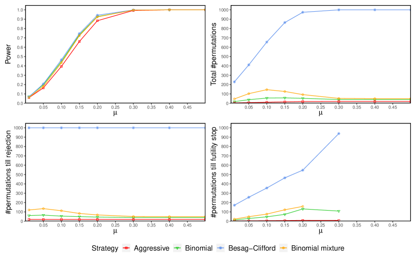
Figure 2: Power and average number of permutations until the decision was obtained for $\alpha=0.05$ and different strengths of the alternative $\mu$ — following the experimental protocol in Subsection 6.2. Upper left plot: Empirical power; Upper right plot: Average number of permutations $\bar{\tau}$; Lower left plot: Average number of permutations until it was stopped for rejection $\bar{\tau}_{1}$; Lower right plot: Average number of permutations until it was stopped for futility $\bar{\tau}_{0}$. Relationship between the plots is given by $\bar{\tau}=(\bar{\tau_{1}}m_{1}+\bar{\tau}_{0}m_{0}+B(m-m_{1}-m_{0}))/m$, where $m_{1}$ and $m_{0}$ are the number of simulation runs where it was stopped for rejection and futility, respectively. The power of binomial strategy and binomial mixture strategy is similar as with Besag-Clifford and number of permutations is reduced substantially, particularly when the alternative is strong.

In line with Figure 1, the power obtained by the binomial strategy and binomial mixture strategy is only slightly worse than the one obtained by Besag-Clifford. However, the number of permutations until a decision is obtained can be reduced a lot by our proposals. In particular, note that the Besag-Clifford strategy only stops earlier for futility, but never in case of a rejection (lower left plots). Therefore, it works well under under the null hypothesis or under very weak alternatives, but under strong alternatives it does not save any computational time compared to the classical approach. In case of $\alpha=0.01$ (Figure 3), the computational gain of our strategies is lower and the power loss of the binomial mixture strategy larger. In the next section, we show that this power loss can be avoided using the stochastic rounding technique described in Section 5.4.

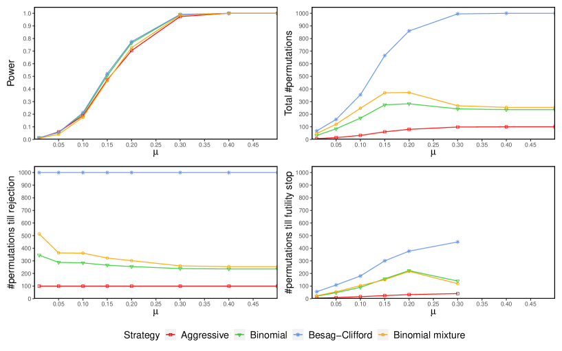
Figure 3: Identical caption as Figure 2, except with $\alpha=0.01$.

6.3 Improving power by stochastic rounding

In this section, we quantify the gain in power obtained by stochastic rounding described in Section 5.4. Note that applying stochastic rounding to the aggressive strategy does not lead to an improvement, since it either rejects or has zero wealth when stopped, which is why we do not include it in this section. The simulation setup is the same as in Section 6.2 and therefore the stopping times are the same as in Figures 2 and 3.

Figure 4 shows that stochastic rounding leads to a significant improvement in power, particularly for the binomial mixture strategy in case of $\alpha=0.01$. This also implies that the binomial mixture strategy was often stopped while having a promising wealth. Therefore, drawing $1000$ permutations might be too less when the $\alpha$ is low and the decision is difficult ($\mathfrak{p}^{\mathrm{lim}}$ close to $\alpha$). Hence, the binomial mixture strategy is likely to achieve further rejections if we would continue sampling. In Figure 5 we compare the power of these randomized strategies with the Besag-Clifford method. There is hardly any power difference visible. In particular, the Besag-Clifford method and randomized binomial mixture strategy seem to overlap completely. Note that our methods obtained this power while reducing the number of permutations considerably (Figure 2 and Figure 3) and offering the option to stop at any point in time.

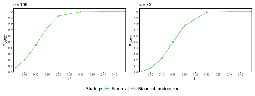
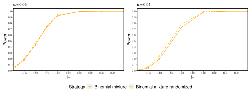
Figure 4: Power comparison of randomized and non-randomized strategies for different significance levels $\alpha$ and strengths of the alternative $\mu$ — following the experimental protocol in Subsection 6.3. The most significant power gain by the randomized strategies is obtained in the cases where the power loss compared to Besag-Clifford was largest (compare to Figure 2 and 3).

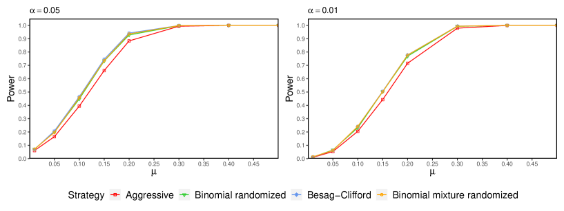
Figure 5: Power of randomized strategies and Besag-Clifford for different significance levels $\alpha$ and strengths of the alternative $\mu$ — following the experimental protocol in Subsection 6.3. The power of the randomized improvements of the binomial and binomial mixture strategy is very similar to the power obtained by Besag-Clifford, while the number of permutations is reduced significantly (see Figure 2 and 3).

6.4 Real data: testing Fisher’s sharp null

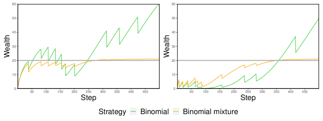
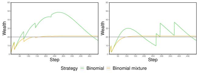
Figure 6: Wealth processes of the binomial strategy and binomial mixture strategy when applied on a real treatment vs. control trial for different runs — following the experimental protocol in Subsection 6.4. The grey horizontal line equals $1/\alpha$. At the beginning the increase in wealth is similar for both strategies. As the wealth of the binomial mixture strategy approaches the level $1/\alpha$, it begins to bet less aggressively (as expected).

We consider a treatment vs. control trial with binary outcomes that was already used in [7, 23]. There were 18 successes among the 32 treated observations and 5 successes among the 21 control observations. We are interested in testing Fisher’s sharp null hypothesis of no individual treatment effect $H_{0}^{\mathrm{IT}}$ at level $\alpha=0.05$. Fisher’s exact test offers a p-value of $0.026$ and thus the null hypothesis could be rejected by this test. We applied our binomial strategy (Algorithm 2) and binomial mixture strategy with density $u_{c}$, $c=0.95\alpha$, $1000$ times with a maximum number of $B=5000$ permutations. In this case, we omitted the stop for futility to not affect the power. The null hypothesis was rejected by both strategies in all $1000$ runs. The binomial strategy needed a mean number of $85$ permutations and a median number of $53$ permutations, while the binomial mixture strategy required a mean number of $147$ permutations and median number of $97$ permutations to obtain the decision. We illustrated the wealth processes of different runs for the first $500$ steps in Figure 6. Since the binomial mixture strategy converges to $1/c$, we expect it to bet more safely when it approaches $1/\alpha$. For this reason, the binomial strategy allows to reject the hypothesis earlier in most cases. However, when there are a lot of losses, e.g. as in the beginning of the upper right plot, the binomial mixture strategy leads to a larger wealth and thus seeming more promising when the evidence is not very strong. Also note that when the number of wins is much larger than the number of losses, as in the lower plots, the binomial strategy begins to lose wealth when further wins occur — after the hypothesis is already rejected. Due to (7), this is the case if $\mathrm{rank}(Y_{0};Y_{0}^{t-1})/(t+1)<p$, where $p=1/\lceil\sqrt{2\pi e^{1/6}}/\alpha\rceil$.

It might seem redundant to reduce the number of permutations in this simple example, since it is not computationally expensive anyway. However, computational cost can be a serious issue in causal inference, particularly when rerandomization is needed [17]. To balance previously observed covariates between treatment groups, patients are often randomized multiple times until some prespecified balance criterion is met. In order to obtain an unbiased test for $H_{0}^{\mathrm{IT}}$, the same criterion need to apply for each of the permuted datasets. Thus, each permutation is checked for its acceptability and unacceptable permutations are discarded. This intermediate check can be very costly and lead to an enormous increase of the required number of permutations, especially when the number of covariates is large and/or the balance criterion is strict. Since the covariate balance is better with stricter criteria, reducing the number of permutations helps with balancing covariates between treatment groups [18].

6.5 Real data: testing conditional independence under model-X

Here, we consider testing the independence between two variables $W$ and $X_{0}$ conditional on some covariates $Z$, denoted by

$$H_{0}^{\mathrm{CI}}:W\mathchoice{\mathrel{\hbox to0.0pt{$\displaystyle\perp$\hss}\mkern 2.0mu{\displaystyle\perp}}}{\mathrel{\hbox to0.0pt{$\textstyle\perp$\hss}\mkern 2.0mu{\textstyle\perp}}}{\mathrel{\hbox to0.0pt{$\scriptstyle\perp$\hss}\mkern 2.0mu{\scriptstyle\perp}}}{\mathrel{\hbox to0.0pt{$\scriptscriptstyle\perp$\hss}\mkern 2.0mu{\scriptscriptstyle\perp}}}X_{0}\ |\ Z.$$

Candès et al. [5] proposed to test $H_{0}^{\mathrm{CI}}$ using a conditional randomization test (CRT) that requires the distribution of $X_{0}|Z$ to be known, which is also known as the model-X assumption. For example, this is a reasonable assumption when a lot of unlabeled realizations of $(X_{0},Z)$ (without the corresponding $W$) are available that can be used as training data to estimate the distribution of $X_{0}|Z$. Let $X_{1},\ldots,X_{B}$ be sampled independently from the distribution of $X_{0}|Z$ and $Y_{i}:=T(W,X_{i},Z)$, $i\in\{0,1,\ldots,B\}$, for an arbitrary test statistic $T$. The test statistics $Y_{1},\ldots,Y_{B}$ are always exchangeable conditional on $Y_{0}$, while $Y_{0},Y_{1},\ldots,Y_{B}$ are exchangeable under $H_{0}^{\mathrm{CI}}$, matching the setting of our paper. The CRT essentially calculates the classical permutation p-value $\mathfrak{p}^{\mathrm{perm}}$ on $Y_{0},\ldots,Y_{B}$. However, generating samples from $X_{0}|Z$ can be computationally challenging or recalculating the test statistic on these samples can be very costly, so a lot of computational effort can potentially be saved by using our sequential permutation tests.

We follow the analysis by Grünwald et al. [11] and Berrett et al. [2] and apply our methods on the Capital bikeshare dataset, which is available at https://ride.capitalbikeshare.com/system-data. In this example, $X_{0}$ denotes the logarithm of the ride duration, $W$ the binary variable membership (casual users vs. long-term membership) and $Z$ is the three dimensional vector of starting point, destination and starting time. For the generation of the test statistics $Y_{0},\ldots,Y_{B}$, we used the code of Grünwald et al. [11], which is available in the supplementary material of their paper. The distribution $X_{0}|Z$ is modeled as Gaussian $N(\mu_{Z},\sigma_{Z}^{2})$, where $\mu_{Z}$ and $\sigma_{Z}^{2}$ are estimated by a kernel regression of $X_{0}$ with the time of day as covariate, separately for each combination of starting point and destination. The test statistics are then given by $Y_{i}=|\mathrm{cor}(W,X_{i}-\mathbb{E}[X_{0}|Z])|$.

We applied our binomial strategy and binomial mixture strategy $1000$ times with the same parameters as in Section 6.4 (in particular, the type I error level was set to 0.05). In the original code of Grünwald et al. [11], the training dataset consists of $158,741$ observations and the test data of $7,173$ observations. In this case, all $Y_{i}$, $i\geq 1$, were smaller than $Y_{0}$ such that the binomial strategy needed $44$ permutations and the binomial mixture strategy $61$ permutations to reject the null hypothesis. We also applied our methods when only the first $2000$ observations of the test data were included, thus increasing the probability of $Y_{i}$ being greater or equal than $Y_{0}$. This led to a mean permutation p-value of $0.008$ and the null hypothesis was still rejected by both sequential strategies in all $1000$ runs. The binomial strategy needed a mean number of $49$ permutations and a median number of $44$ permutations, while the binomial mixture strategy required a mean number of $83$ permutations and median number of $61$ permutations to obtain the decision.

7 Discussion

We have introduced a new test martingale for exchangeability based on a simple testing by betting approach. In contrast to previous works we focused on the alternative that all test statistics are exchangeable except the first. This alternative is motivated by permutation tests, where the observed data is fixed and additional data is generated that is supposed to have the same distribution as the original data under the null hypothesis. We derived the log-optimal betting strategy under the considered alternative and showed that the corresponding wealth does not grow exponentially, which distinguishes our problem from many others. Furthermore, we showed that for any given prior on the limiting permutation p-value $\mathfrak{p}^{\mathrm{lim}}$, the log-optimal strategy can be written as a mixture of simple binomial strategies. Based on this, we proposed a strategy with zero resampling risk after a finite number of permutations for all $p^{\mathrm{lim}}\in[0,c)$, where $c<\alpha$ can be chosen arbitrarily close to $\alpha$. Furthermore, we performed a simulation study and a real data analysis which illustrates that our anytime-valid p-values have a similar power as the classical permutation p-value while the number of permutations until the decision is obtained can be substantially reduced.

	Pros	Cons
Aggressive strategy	•  Requires least possible permutations •  Parameter-free	•  Weak result regarding     •   resampling risk •  Slightly less power than the     •   other strategies
Binomial strategy	•  Reduces permutations substantially •  Similar power as classical permutation     •   p-value in all simulation scenarios •  Always rejects earlier than classical     •   permutation p-value, if     •   $\mathfrak{p}^{\mathrm{perm}}<1/\lceil\sqrt{2\pi e^{1/6}}/\alpha\rceil\approx\alpha/e$     •   (Proposition 4.4) •  Parameter-free (see Algorithm 2)	•  Cannot ensure arbitrarily     •   small resampling risk
Binomial mixture strategy	•  Reduces permutations substantially •  Nearly identical power as classical     •   permutation p-value in simulations     •   after stochastic rounding •  Can keep resampling risk arbitrarily     •   small (see Corollary 5.4 and 5.5) •  Parameter $c\in[0,1]$ has simple     •   interpretation with respect to     •   asymptotic behavior (Theorem 5.3) •  Wealth is decreasing in number     •   of losses •  Theoretically most grounded strategy	•  Slightly lower power     •   than the binomial strategy     •   in the simulations without     •   stochastic rounding

Table 1: Pros and cons of the proposed betting strategies.

In Table 1 we list the pros and cons of the proposed betting strategies. To summarize, the aggressive strategy should be used when one is mainly concerned with reducing the number of permutations and a (small) loss of power can be accepted in return. However, in most cases the binomial and binomial mixture strategies are more appropriate, since they have a (slightly) larger power while still keeping the number of permutations quite low. If stochastic rounding is accepted, the binomial mixture strategy should be used, since it is the theoretically most grounded strategy and led to the best performance after the randomization. If stochastic rounding should be avoided, both the binomial and binomial mixture strategies are reasonable. The binomial strategy tends to stop earlier, while the binomial mixture strategy offers a better asymptotic behavior and can be used to bound the resampling risk.

In future work, we hope to explore applications of our approach to multiple testing.

Acknowledgments

AR thanks Leila Wehbe for posing the question of whether permutation tests can be stopped early under null and alternative, and for stimulating practical discussions. LF acknowledges funding by the Deutsche Forschungsgemeinschaft (DFG, German Research Foundation) – Project number 281474342/GRK2224/2. AR was funded by NSF grant DMS-2310718.

Appendix A More details on (orthogonally) related work

For the particular problem of testing our null hypothesis that the observations are exchangeable, there exists no nontrivial test martingale for the canonical data filtration (generated by the observations) [20]. There are two different approaches to circumvent this issue. The first idea is to replace the data filtration by a coarser one. This means the information to be released at each step is restricted. This was used by Vovk and colleagues in a conformal prediction approach [31, 29], and this is also the approach taken in the current paper (modulo some differences around randomization of ranks). The second approach is to construct an e-process which is not a test martingale, based on universal inference [33, 20]. The idea is to partition the composite null hypothesis, define a test martingale for each subset and take the infimum over these test martingales to yield an e-process. In terms of testing by betting, it could be interpreted as playing multiple games, where the gambler’s wealth is the minimum wealth across all these games. In this case, the wealth process is adapted to the canonical data filtration, has expectation of at most one under the null at any stopping time in the original filtration of the data.

Very recently, other sequential tests of exchangeability were proposed, based on the former approach. Saha and Ramdas [24] introduced a test martingale for Markovian alternatives that is based on “pairwise betting”, which means that two observations are observed and bet on simultaneously. Independently, Koning [16] introduced a sequential test for general group invariance (including exchangeability). In particular, he derives likelihood ratios for group invariance and defines a test martingale as running product of these. Our test martingale is also based on coarsening the data filtration by not revealing the $Y_{t}$ itself, but the rank among the previously known observations, and is thus somewhat related to this line of work. The main difference of our approach to the previously mentioned approaches is the alternative we test against. Vovk [29] focuses on change-point alternatives, Ramdas et al. [20] and Saha and Ramdas [24] on Markovian alternatives, while Koning [16] considers general group invariance versus normal distributions with a location shift. In contrast, our paper focuses on the usual setting of permutation tests (where permutations rather than data are sampled sequentially), where under the alternative, only the original test statistic is special while all the permuted statistics are exchangeable by design.

Appendix B Calibrating $\mathfrak{p}^{\mathrm{perm}}_{B}$ into an e-value

An e-value $E$ is a random variable with expectation less than one under the null hypothesis. For example, our test martingale $W_{\tau}$ is an e-value for each stopping time $\tau$. A (non-random) function $h$ such that $h(E)$ is a p-value, where $E$ is an e-value, is called e-to-p calibrator. We have already argued in Section 2 that $h(E)=1/E$ is an e-to-p calibrator. It can even even be shown that $h$ is the only admissible e-to-p calibrator, which means that there exists no other e-to-p calibrator $g$ with $g\geq h$ and $g\neq h$ [30]. Note that we restrict to non-random calibrators $h$. Otherwise, $h(E)=1/E$ could be improved by $\tilde{h}(E)=U/E$, where $U$ is standard uniformly distributed and independent of $E$. The fact that $\tilde{h}(E)$ defines a valid p-value follows from a randomized improvement of Markov’s inequality [19].

Analogously, we can define p-to-e calibrators (in the following, we just call these calibrators). However, in this case there are many more possible choices of calibrators. Below, we show that classical calibrators are inadmissible in our setting and introduce a new class of admissible calibrators for such problems. Furthermore, since calibrators define betting strategies, we show that classical calibrators lead to strategies with low power by means of simulations.

Vovk and Wang [30] showed that a decreasing function $h$ is an admissible calibrator if and only if $h$ is upper semicontinuous, $h(0)=0$ and $\int_{0}^{1}h(u)du=1$. However, this result is restricted to continuous p-values while the permutation p-value $\mathfrak{p}^{\mathrm{perm}}_{B}$ only takes on discrete values. For example, a simple and often used calibrator class satisfying the above conditions is given by $h(p)=\kappa p^{\kappa-1}$ for some $\kappa\in(0,1)$. Note that, e.g., for $\kappa=1/2$ and $B=2$, we have

$$\mathbb{E}[h(\mathfrak{p}^{\mathrm{perm}}_{B})]=\frac{1}{3}\frac{1}{2}\sqrt{3}+\frac{1}{3}\frac{1}{2}\sqrt{\frac{3}{2}}+\frac{1}{3}\frac{1}{2}\sqrt{1}=\frac{1}{6}\left(\sqrt{3}+\sqrt{\frac{3}{2}}+1\right)<1,$$

which shows that $h$ is inadmissible in this case. In the following we provide a characterization of admissible calibrators for p-values with the same support as $\mathfrak{p}^{\mathrm{perm}}_{B}$.

Proposition B.1.

Let $\mathfrak{p}^{\mathrm{perm}}_{B}$ be a p-value with support $\{1/(B+1),\ldots,B/(B+1),1\}$ and $\mathbb{P}(\mathfrak{p}^{\mathrm{perm}}_{B}\leq r/(B+1))=r/(B+1)$ for all $1\leq r\leq B+1$. The calibrator $h$ is admissible for $\mathfrak{p}^{\mathrm{perm}}_{B}$ if and only if $\sum_{r=1}^{B+1}h(r/(B+1))=B+1$.

Proof.

The proposition follows immediately from $\mathbb{E}[h(\mathfrak{p}^{\mathrm{perm}}_{B})]=\sum_{r=1}^{B+1}h(r/(B+1))/(B+1)$ under the null hypothesis. ∎

An example of an admissible calibrator for $\mathfrak{p}^{\mathrm{perm}}_{B}$ is

$$h(\mathfrak{p}^{\mathrm{perm}}_{B})=h(r/(B+1))=(B+1)/(r\ell_{B+1}),\quad 1\leq r\leq B+1,$$ (9)

where $\ell_{B}=1+1/2+1/3+\dots 1/B$ is the $B$-th harmonic number. This is reminiscent of the Benjamini-Yekutieli correction in multiple testing [1]. Indeed, if these e-values (calibrated p-values) are plugged into the e-BH procedure [32], one obtains a method that is equivalent to applying the BY procedure on the original p-values.

Another option is to define

$$h(\mathfrak{p}^{\mathrm{perm}}_{B})=h(r/(B+1))=\frac{(B+1)/\sqrt{r}}{s_{B+1}}>\sqrt{B+1}/(2\sqrt{r})=1/(2\sqrt{\mathfrak{p}^{\mathrm{perm}}_{B}}),$$ (10)

where $s_{B+1}=\sum_{i=1}^{B+1}1/\sqrt{i}<2\sqrt{B+1}-1$, which shows that this is a uniform improvement of the calibrator by Vovk and Wang [30] for $\kappa=1/2$.

Note that $R_{B}/(B+1)$, where $R_{B}$ is the rank of the $B$-th permutation, is also a valid p-value under the null hypothesis with the same support as $\mathfrak{p}^{\mathrm{perm}}_{B}$, even conditional on the ranks of the previous permutations $R_{1}^{B-1}$. Also note that the condition derived in Proposition B.1 is exactly the same as we derived for our betting strategies in Section 1.1. Therefore, every admissible calibrator $h$ for $\mathfrak{p}^{\mathrm{perm}}_{B}$ defines a bet $B_{B}$ on the rank $R_{B}$ and vice versa. Hence, one approach to find betting strategies would be to just use the calibrators from 9 or 10. Note that the calibrators should be applied to the “p-value” $(B-R_{B}+2)/(B+1)$ instead of $R_{B}/(B+1)$, such that small values are evidence for the alternative.

In Figure 7, the power and number of permutations is displayed for the betting strategies obtained by the calibrators from  9 and 10 and for our binomial strategy. We used the same simulation setup as in Section 6. It is easy to see that the power of the calibration based strategies is very low. This exemplifies the importance of adapting the betting strategy to the previous ranks.

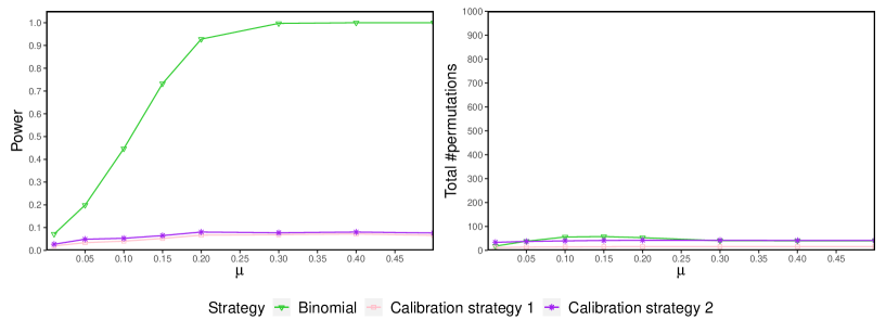
Figure 7: Power and number of permutations until the decision was obtained for $\alpha=0.05$ and different strengths of the alternative $\mu$.

Appendix C Using a Beta distribution as prior for $\mathfrak{p}^{\mathrm{lim}}$

A common prior for the probability in a Bernoulli trial is a beta distribution. The probability density function of a beta distribution for shape parameters $a,b>0$ is given by

$$g_{a,b}(x)=\frac{x^{a-1}(1-x)^{b-1}}{\mathrm{Beta}(a,b)},\text{ where }\mathrm{Beta}(a,b)=\int_{0}^{1}u^{a-1}(1-u)^{b-1}du\quad(0\leq x\leq 1).$$

The function $\mathrm{Beta}(a,b)$ is called beta function. In this section we derive the wealth obtained by applying the binomial mixture strategy with a beta distribution as prior for $\mathfrak{p}^{\mathrm{lim}}$ and show some simulation results for this strategy.

Proposition C.1.

After $B$ permutations and $k$ losses, the wealth obtained by the binomial mixture strategy with density $g_{a,b}$ is given by $W_{B}^{g_{a,b}}(k)=\mathrm{Beta}(a+k,b+B-k)/(\mathrm{Beta}(k+1,B-k+1)\mathrm{Beta}(a,b))$.

Proof.

First note that $(B+1){B\choose k}=\mathrm{Beta}(k+1,B+1)$. Therefore, the wealth is given by

$$W_{B}^{g_{a,b}}(k) =(B+1){B\choose k}\int_{0}^{1}p^{k}(1-p)^{B-k}g_{a,b}(p)dp$$

$$=(B+1){B\choose k}\frac{\int_{0}^{1}p^{k+a-1}(1-p)^{B+b-k-1}dp}{\mathrm{Beta}(a,b)}$$

$$=\frac{\mathrm{Beta}(k+a,B+b-k)}{\mathrm{Beta}(k+1,B-k+1)\mathrm{Beta}(a,b)}.$$

∎

It can be shown that if $a\leq 1$ and $b\geq 1$, then $g_{a,b}(x)$ is nonincreasing in $x$ which seems reasonable as prior for $\mathfrak{p}^{\mathrm{lim}}$. In particular, for $a=1$ and $b\in\mathbb{N}$, the wealth simplifies to

$$W_{B}^{g_{1,b}}(k)=b\frac{(B+1)\cdots(B-k+1)}{(B+b)\cdots(B-k+b)},$$

which is decreasing for an increasing number of losses. In Figure 8 the log-transformed p-values obtained by the binomial mixture strategy with density $g_{1,b}$ are compared with the ones obtained by the binomial strategy, the binomial mixture strategy (with density $u_{0.9\alpha}$), the aggressive strategy and the classical permutation p-value. We used the same simulation setup as described in Section 6. The binomial mixture strategy with beta prior bets more aggressively when $b$ is large. However, the binomial strategy and the binomial mixture strategy with uniform prior lead to more rejections, as seen by the larger number of log-transformed p-values below the grey line $\log(\alpha)$, in all cases.

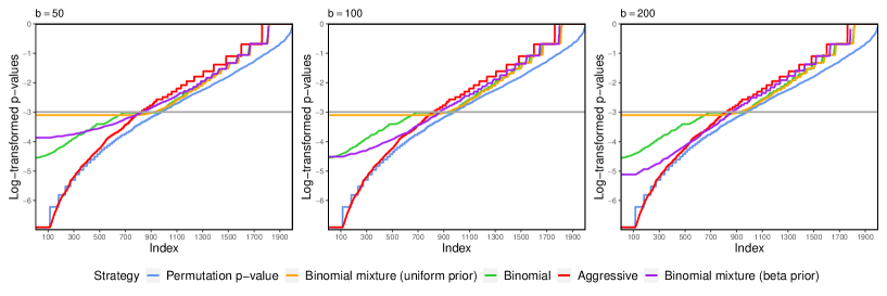
Figure 8: All plots display log-transformed p-values in ascending order for $2000$ simulations — following the experimental protocol in Subsection C. The grey horizontal line equals $\log(\alpha)$, where $\alpha$ equals 0.05. The binomial mixture strategy with a beta prior bets more aggressive when $b$ is large. However, in terms of rejections (p-values below grey line) it is outperformed by the binomial strategy and the binomial mixture strategy with uniform prior in all cases.

References

- Benjamini and Yekutieli [2001] Yoav Benjamini and Daniel Yekutieli. The control of the false discovery rate in multiple testing under dependency. Annals of Statistics, pages 1165–1188, 2001.
- Berrett et al. [2020] Thomas B Berrett, Yi Wang, Rina Foygel Barber, and Richard J Samworth. The conditional permutation test for independence while controlling for confounders. Journal of the Royal Statistical Society Series B: Statistical Methodology, 82(1):175–197, 2020.
- Besag and Clifford [1991] Julian Besag and Peter Clifford. Sequential Monte Carlo p-values. Biometrika, 78(2):301–304, 1991.
- Breiman [1961] Leo Breiman. Optimal gambling systems for favourable games. In Fourth Berkeley Symposium on Mathematical Statistics and Probability, pages 65–78, 1961.
- Candès et al. [2018] Emmanuel Candès, Yingying Fan, Lucas Janson, and Jinchi Lv. Panning for gold:‘model-x’knockoffs for high dimensional controlled variable selection. Journal of the Royal Statistical Society Series B: Statistical Methodology, 80(3):551–577, 2018.
- Cover [1999] Thomas M Cover. Elements of information theory. John Wiley & Sons, 1999.
- Ding [2017] Peng Ding. A paradox from randomization-based causal inference. Statistical Science, pages 331–345, 2017.
- Fay and Follmann [2002] Michael P Fay and Dean A Follmann. Designing Monte Carlo implementations of permutation or bootstrap hypothesis tests. The American Statistician, 56(1):63–70, 2002.
- Fay et al. [2007] Michael P Fay, Hyune-Ju Kim, and Mark Hachey. On using truncated sequential probability ratio test boundaries for Monte Carlo implementation of hypothesis tests. Journal of Computational and Graphical Statistics, 16(4):946–967, 2007.
- Gandy [2009] Axel Gandy. Sequential implementation of Monte Carlo tests with uniformly bounded resampling risk. Journal of the American Statistical Association, 104(488):1504–1511, 2009.
- Grünwald et al. [2023] Peter Grünwald, Alexander Henzi, and Tyron Lardy. Anytime-valid tests of conditional independence under model-X. Journal of the American Statistical Association, pages 1–12, 2023.
- Grünwald et al. [2024] Peter Grünwald, Rianne de Heide, and Wouter M Koolen. Safe testing. Journal of the Royal Statistical Society Series B: Statistical Methodology (with discussion), 2024.
- Howard et al. [2021] Steven R Howard, Aaditya Ramdas, Jon McAuliffe, and Jasjeet Sekhon. Time-uniform, nonparametric, nonasymptotic confidence sequences. Annals of Statistics, 2021.
- Johari et al. [2022] Ramesh Johari, Pete Koomen, Leonid Pekelis, and David Walsh. Always valid inference: Continuous monitoring of A/B tests. Operations Research, 70(3):1806–1821, 2022.
- Kelly [1956] John L Kelly. A new interpretation of information rate. The Bell System Technical Journal, 35(4):917–926, 1956.
- Koning [2023] Nick W Koning. Online permutation tests and likelihood ratios for testing group invariance. arXiv preprint arXiv:2310.01153, 2023.
- Morgan and Rubin [2012] Kari Lock Morgan and Donald B Rubin. Rerandomization to improve covariate balance in experiments. The Annals of Statistics, 40(2):1263–1282, 2012.
- Morgan and Rubin [2015] Kari Lock Morgan and Donald B Rubin. Rerandomization to balance tiers of covariates. Journal of the American Statistical Association, 110(512):1412–1421, 2015.
- Ramdas and Manole [2023] Aaditya Ramdas and Tudor Manole. Randomized and exchangeable improvements of Markov’s, Chebyshev’s and Chernoff’s inequalities. arXiv preprint arXiv:2304.02611, 2023.
- Ramdas et al. [2022] Aaditya Ramdas, Johannes Ruf, Martin Larsson, and Wouter M Koolen. Testing exchangeability: Fork-convexity, supermartingales and e-processes. International Journal of Approximate Reasoning, 141:83–109, 2022.
- Ramdas et al. [2023] Aaditya Ramdas, Peter Grünwald, Vladimir Vovk, and Glenn Shafer. Game-theoretic statistics and safe anytime-valid inference. Statistical Science, 38(4):576–601, 2023.
- Rényi [1962] A Rényi. On the extreme elements of observations. MTA III. Oszt. Közl, 12:105–121, 1962.
- Rosenbaum [2002] Paul R Rosenbaum. Observational Studies. Springer, 2002.
- Saha and Ramdas [2023] Aytijhya Saha and Aaditya Ramdas. Testing exchangeability by pairwise betting. arXiv preprint arXiv:2310.14293, 2023.
- Shafer [2021] Glenn Shafer. Testing by betting: A strategy for statistical and scientific communication. Journal of the Royal Statistical Society Series A: Statistics in Society (with discussion), 184(2):407–431, 2021.
- Shafer et al. [2011] Glenn Shafer, Alexander Shen, Nikolai Vereshchagin, and Vladimir Vovk. Test martingales, Bayes factors and p-values. Statistical Science, 2011.
- Silva et al. [2009] Ivair Silva, Renato Assunçao, and Marcelo Costa. Power of the sequential Monte Carlo test. Sequential Analysis, 28(2):163–174, 2009.
- Silva and Assunção [2013] Ivair R Silva and Renato M Assunção. Optimal generalized truncated sequential Monte Carlo test. Journal of Multivariate Analysis, 121:33–49, 2013.
- Vovk [2021] Vladimir Vovk. Testing randomness online. Statistical Science, 36(4):595–611, 2021.
- Vovk and Wang [2021] Vladimir Vovk and Ruodu Wang. E-values: Calibration, combination and applications. The Annals of Statistics, 49(3):1736–1754, 2021.
- Vovk et al. [2005] Vladimir Vovk, Alexander Gammerman, and Glenn Shafer. Algorithmic learning in a random world, volume 29. Springer, 2005.
- Wang and Ramdas [2022] Ruodu Wang and Aaditya Ramdas. False discovery rate control with e-values. Journal of the Royal Statistical Society Series B: Statistical Methodology, 84(3):822–852, 2022.
- Wasserman et al. [2020] Larry Wasserman, Aaditya Ramdas, and Sivaraman Balakrishnan. Universal inference. Proceedings of the National Academy of Sciences, 117(29):16880–16890, 2020.
- Waudby-Smith and Ramdas [2020] Ian Waudby-Smith and Aaditya Ramdas. Confidence sequences for sampling without replacement. Advances in Neural Information Processing Systems, 33:20204–20214, 2020.
- Waudby-Smith and Ramdas [2023] Ian Waudby-Smith and Aaditya Ramdas. Estimating means of bounded random variables by betting. Journal of the Royal Statistical Society Series B: Statistical Methodology (with discussion), 2023.
- Xu and Ramdas [2023] Ziyu Xu and Aaditya Ramdas. More powerful multiple testing under dependence via randomization. arXiv preprint arXiv:2305.11126, 2023.