Analysis of Performance Limits in Current-Matched Tandem Solar Cells

Abstract

Our work estimates the performance limits of an $N$-layer current-matched (CM) tandem solar cell with and without subcells/modules in each layer, accounting for radiative coupling between the layers. Current matching constraints are alleviated with the help of adding additional modules at each layer appropriately. The optimal number of subcells to achieve maximum efficiency is also determined. This model serves as a general framework for the analysis of efficiency limits and provides design insights into the number of subcells/modules of any number of layers and can be extended to voltage-matched (VM) devices and bifacial devices as well.

1 Introduction

The transition to renewable energy sources is of paramount importance in the global strategy to combat climate change and achieve sustainability. At the forefront of this transition is photovoltaic (PV) technology, which has seen rapid growth in both research and deployment. They are pivotal in reducing the carbon footprint and curbing our dependence on fossil fuels [1, 2, 3]. The Paris Agreement and subsequent policy initiatives like the European Green Deal have set ambitious targets to reduce carbon emissions [4, 5]. A recent study by Ernst & Young claims that the Levelized Cost of Electricity (LCOE) for PV is now $29\%$ lower than the cheapest fossil fuel alternative [6]. In this context, advancing the efficiency and effectiveness of solar technologies is not just a scientific challenge but a necessity for meeting these global environmental goals as well. Emergent technologies such as the field of agrophotovoltaics are a promising avenue of research as incorporating solar energy harvesting and agricultural production within the same area optimizes land usage [7].

The technological evolution of PV cells from traditional single-junction (SJ) to advanced multi-junction (MJ) configurations is reflective of the industry’s response to the dual challenges of efficiency and economic viability. As SJ solar cells have been approaching the Shockley-Queisser (SQ) limit [8], it has prompted the exploration of different designs, such as different tandem configurations, which have the potential to capture a broader spectrum of solar radiation [9, 10, 11]. Therefore, improving the performance of tandem solar cells is of particular interest as they have the potential for higher efficiencies and power outputs, due to their increased utilization of the solar spectrum [12]. Current-matched (CM) tandem (two-terminal tandem) cells, in particular, are popular owing to their relative ease of fabrication in contrast to unconstrained and voltage-matched (VM) configurations. However, their performance is constrained by requiring the current densities to be the same across the layers, limiting the current density to the cell with the lowest current density. An approach to alleviate this constraint is to add subcells/modules at each layer, such that the current densities across layers are matched [13, 14].

Predominantly, the existing literature focuses on two-layer CM tandems [13, 15, 16, 17], with a primary focus on material synthesis and advancements in the fabrication of these devices (such as, performance enhancement observed in different perovskite-based tandem cells). There have been a few reports on analyzing two-layer CM and VM tandems [13, 18]. However, there are no reports, yet, that discuss the performance limits of CM tandems with more than two layers, and that calculate the optimal number of subcells across different layers. While an analytical expression has been derived in [18] to determine the optimal number of subcells in VM devices, there has been no analytical framework providing the same for CM tandems.

This work provides a general analytical framework, employing the principle of detailed balance [19], for modeling $N$-layer CM tandem solar cells with subcells/modules, accounting for radiative coupling across the layers, and determining the optimal number of subcells/modules to be chosen in each layer, to achieve the maximum efficiency. This paper is organized as follows: after describing the device configuration in the next section, we expand on our modeling approach and present our calculations and analysis in the subsequent sections. Finally, we discuss the scope and limitations of this approach and furnish our concluding remarks.

2 Device Structure

The schematic of an $N$-layer CM tandem cell is shown in Fig. 1; $N$ is the number of layers, and $m_{i}$ is the number of subcells/modules in layer $i$. We have assumed the presence of a back reflector at the bottom of layer $1$. Each layer (indicated by a specific colour), can have many subcells/modules that are connected in series; the layers, in turn, are connected in series as well. All the layers are assumed to have the same area, which means that the individual subcells/modules across different layers need not have the same area. The spacing between adjacent subcells and layers is assumed to be negligible.

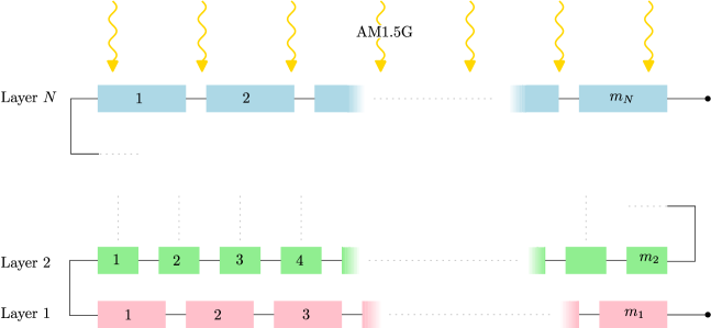
Figure 1: Schematic of a typical device configuration of an $N$-layer CM tandem cell with subcells.

3 Modeling Approach

Our approach uses the principle of detailed balance; this work assumes radiative recombination as the exclusive loss mechanism, and that the solar cell acts as a black body that inherently emits radiation. The current density lost due to this process in a SJ cell of band gap $E_{g}$ emitted towards both hemispheres is given by [20, 21]:

Figure 2: Flowchart summarising our framework.

$$J_{dark}=J_{0}\exp\left({\frac{qV}{kT}}\right)$$ (1)

where, $J_{0}$ is given by,

$$J_{0}=q\int_{E_{g}}^{\infty}\frac{4\pi}{{c^{2}h^{3}}}E^{2}\exp\left(\frac{-E}{kT}\right)dE$$ (2)

$V$ is the voltage, $T$ is the temperature, $k$ is the Boltzmann constant, $q$ is the charge of an electron, $h$ is Planck’s constant, and $c$ is the speed of light in vacuum. We have used the AM1.5G spectrum as the incident solar spectrum. The photon flux above a certain bandgap is calculated by integrating the photon flux over the energy spectrum, starting from the energy corresponding to the bandgap to the maximum available energy. This determines the number of photogenerated carriers that contribute to the photonic current density, $J_{ph}$. Thus, the effective current for a SJ solar cell is given by the difference in photonic and dark current densities, that is ($J_{ph}-J_{dark}$) [18]:

$$J=J_{ph}-J_{0}\cdot\exp{\left(V/V_{t}\right)}$$ (3)

where, $V_{t}$ is the thermal voltage given by $kT/q$.

For the $N$-layer CM tandem device configuration, shown in Fig. 1, each subcell can be considered as a SJ device. The current density in layer $i$ is given by:

$$J_{i}=\frac{J_{ph,i}}{m_{i}}-\frac{J_{0,i}}{m_{i}}\exp\left(\frac{V_{i}}{m_{i}V_{t}}\right)+\frac{J_{0,i+1}}{2m_{i}}\exp\left(\frac{V_{i+1}}{m_{i+1}V_{t}}\right)$$ (4)

Each individual subcell in layer $i$ contributes a voltage of ${V_{i}}/{m_{i}}$ which gives a total voltage $V_{i}$ for that layer. As the device is in series configuration, these voltages add up to give $\mathbf{V}$. As the photonic flux gets scaled, the photonic current density gets scaled as well. Similarly, the radiative coupling and dark current densities are scaled by the number of subcells in the corresponding layer.

Optimization of the number of subcells/modules in each layer requires equalizing the current densities at their maximum power point ($MPP$), $J_{mpp}$ across all the layers, as the device is to have the same current across all layers [18]. Thus, the general expression for $m_{i}$ in terms of the number of top-most cells ($m_{N}$) is found to be:

$$m_{i}=\frac{m_{N}}{2^{N-i}}\cdot\left[\frac{\lambda(J_{ph})}{J_{ph,N}}\cdot\frac{\alpha}{\beta}-\frac{\phi(m)}{m_{N}}\right]$$ (5)

where, $\alpha$, $\beta$, $\lambda(J_{ph})$, and $\phi(m)$ are given by:

$$\alpha=1-\frac{1}{W\left(\frac{\lambda(J_{ph})}{2^{N-i}\cdot J_{0,i}}e\right)} \beta=1-\frac{1}{W\left(\frac{J_{ph,N}}{J_{0,N}}e\right)}$$ (6)

$$\lambda(J_{ph})=\sum_{j=0}^{N-i}\left(2^{j}\cdot J_{ph,N-j}\right) \phi(m)=\sum_{j=1}^{N-i}\left(2^{j}\cdot m_{N-j}\right)$$ (7)

where, $W$ is the Lambert $W$ function [22].

The optimal number of bottom subcells ($m_{1}$) for a two-layer CM tandem is given by:

$$m_{1}=\frac{m_{2}}{2}\left[\frac{J_{ph,2}+2J_{ph,1}}{J_{ph,2}}\cdot\frac{\alpha}{\beta}-1\right]$$ (8)

Similarly, for a three-layer CM device, $m_{2}$ and $m_{1}$ are given by

$$m_{2}=\frac{m_{3}}{2}\left[\frac{J_{ph,3}+2J_{ph,2}}{J_{ph,3}}\cdot\frac{\alpha}{\beta}-1\right]$$ (9)

$$m_{1}=\frac{m_{3}}{4}\left[\frac{J_{ph,3}+2J_{ph,2}+4J_{ph,1}}{J_{ph,3}}\cdot\frac{\alpha}{\beta}-\frac{m_{3}+2m_{2}}{m_{3}}\right]$$ (10)

On obtaining the optimal number of subcells across all the layers, an expression for the current density - voltage ($\mathbf{J-V}$) for the complete tandem device can now be constructed. As the device is to be current-matched, the current densities across all layers are equated to $\mathbf{J}$. On solving equation (4) $\forall i\in[1,N]$, a general equation for the $\mathbf{J}-\mathbf{V}$ characteristics for an $N$-layer CM tandem device is obtained:

$$\mathbf{V}=\sum\limits_{i=1}^{N}m_{i}V_{t}\ln\left(\frac{\left(\sum\limits_{j=1}^{i+1}2^{i-j}\cdot J_{ph,j}\right)-\left(\sum\limits_{j=1}^{i+1}2^{i-j}\cdot m_{j}\right)\mathbf{J}}{2^{N-i}\cdot J_{0,i}}\right)$$ (11)

Parameters such as the open circuit voltage ($V_{oc}$), short circuit current density ($J_{sc}$), voltage at $MPP$ ($V_{mpp}$), current density at $MPP$ ($J_{mpp}$), fill factor ($FF$) and efficiency ($\eta$) can now be calculated from the tandem’s $\mathbf{J-V}$ characteristics. Our framework is summarised in the flowchart shown in Fig. 2.

4 Results and Discussion

The model’s efficacy is demonstrated using two-layer and three-layer CM tandem devices as a case study. Fig. 3 and 4 summarise the results from our calculations for a two-layer and three-layer CM tandem cell, respectively.

Fig. 3(a) and (b) illustrate the $\eta$ and $FF$ of the device in the absence of subcells, that is, when $m_{2}=m_{1}=1$. It is observed that a small range of bandgap combinations of top and bottom layers yield high efficiencies. Additionally, it is discernible from Fig. 3(b) that the bandgap combinations that yield maximum $\eta$ does not correspond to the ones that give maximum $FF$; this is due to the latter’s dependency on $V_{mpp},J_{mpp},V_{oc}$, and $J_{sc}$ [23].

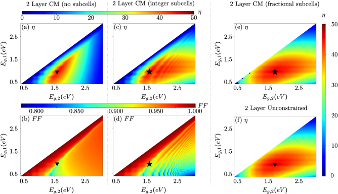
Figure 3: (a)-(d) $\eta$ and $FF$ as a function of bandgaps ($E_{g,2},E_{g,1}$) for two-layer CM tandems: (a)-(b) for configuration without subcells, (a) $\eta$ and (b) $FF$. (c)-(d) for configuration with integer subcells, (c) $\eta$ and (d) $FF$. (e)-(f) $\eta$ as a function of bandgaps ($E_{g,2},E_{g,1}$) for two-layer tandems: (e) for CM configuration with subcells (without integer restriction); (f) for unconstrained configuration. The symbols $\blacktriangledown$ and $\bigstar$ indicate the combination of bandgaps yielding maximum efficiency, for devices without subcells and those with subcells, respectively.

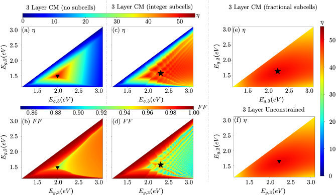
Figure 4: (a)-(d) $\eta$ and $FF$ as a function of bandgaps ($E_{g,3},E_{g,2}$) for three-layer CM tandems: (a)-(b) for configuration without subcells, (a) $\eta$ and (b) $FF$. (c)-(d) for configuration with integer subcells, (c) $\eta$ and (d) $FF$. (e)-(f) $\eta$ as a function of bandgaps ($E_{g,3},E_{g,2}$) for three-layer tandems: (e) for CM configuration with subcells (without integer restriction); (f) for unconstrained configuration. The bottom-most layer in all the configurations is assumed to be $Si$, with $E_{g,1}=1.12eV$. The symbols $\blacktriangledown$ and $\bigstar$ indicate the combination of bandgaps yielding maximum efficiency, for devices without subcells and those with subcells, respectively.

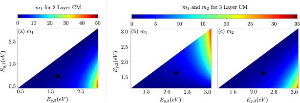
Figure 5: (a)-(c) Optimal number of subcells in CM tandem devices: (a) Optimal number of bottom subcells $m_{1}$ in a two-layer CM tandem. (b) and (c) shows the optimal number of subcells for each layer in a three-layer CM tandem device: (b) shows the optimal number of subcells in layer $1$ ($m_{1}$), and (c) in layer $2$ ($m_{2}$). The bottom-most layer in the three-layer configuration is $Si$ with $E_{g,1}=1.12eV$

Fig. 3(c) and (d) show the $\eta$ and $FF$ plots for devices with subcells, where the optimal number of subcells is determined using equation (5) (subcell counts are rounded off to the nearest natural number). Fig. 5 (a) indicates the optimal number of subcells for the first layer, calculated assuming a single subcell in the top layer (that is, $m_{2}=1$). From Fig. 3 (c), we can observe that the spread of bandgap combinations that yield higher efficiencies has increased. This is to be expected as we are, in essence, alleviating the constraint by adding the appropriate number of subcells/modules to the layer with the lower current density. The jagged/sharp edges in the contour plot is due to the integer restriction imposed on the number of subcells; on removing this restriction, we can see a more uniform spread, as seen in Fig. 3(e).

Unconstrained tandems have higher efficiency limits for a wider range of bandgaps [13, 24] [as seen in Fig. 3(f)], compared to their constrained counterparts without subcells [as seen in Fig. 3(a)]. The inclusion of subcells at each layer of a CM tandem device potentially alleviates the limitations associated with current matching requirements, thereby enhancing performance akin to that of unconstrained counterparts, as shown in Fig. 3(c) and (e).

Table 1: Summary of parameters for different configurations of two-layer tandem devices.

Device Configuration	$E_{g,2},E_{g,1}(eV)$	Maximum $\eta$ ($\%$)	Fill Factor	Subcells ($m_{2},m_{1}$)
Two-layer Unconstrained	$1.73,0.94$	45.94	-	-
Two-layer CM, no subcells	$1.59,0.94$	45.55	0.88	-
Two-layer CM with integer subcells	$1.59,0.94$	45.55	0.88	1,1
Two-layer CM with fractional subcells	$1.73,0.94$	45.90	0.89	1,1.33

Table 2: Summary of parameters for different configurations of three-layer tandem devices.

Device Configuration	$E_{g,3},E_{g,2},E_{g,1}(eV)$	Maximum $\eta$ ($\%$)	Fill Factor	Subcells ($m_{3},m_{2},m_{1}$)
Three-layer Unconstrained	$2.23,1.64,1.12$	49.72	-	-
Three-layer CM, no subcells	$2.00,1.49,1.12$	49.31	0.90	-
Three-layer CM with integer subcells	$2.31,1.58,1.12$	49.53	0.90	1,2,2
Three-layer CM with fractional subcells	$2.23,1.64,1.12$	49.69	0.91	1,1.40,1.87

Table 1 summarizes the performance of two-layer tandem cells with different configurations. The efficiency of a CM tandem with subcells (no integer restriction) exhibits a similar maximum efficiency as that of the unconstrained configuration. While the variation in maximum efficiency limits across different configurations is negligible, there is a significant difference in the selection of bandgaps that yield higher efficiencies. The range of combinations of bandgaps that yield high efficiencies is much larger in CM tandems with subcells [Fig. 3(c) and (e)], as compared to the one without [Fig. 3(a)].

Applying this framework to a three-layer CM tandem device reveals similar patterns. The bottom-most layer is assumed to be silicon having a bandgap of $1.12eV$. The bandgaps of the top and middle layers are varied, and the performance limits are calculated accordingly. Fig. 4(a) shows that there is a smaller combination of bandgaps yielding maximum efficiencies without the addition of subcells. With the addition of subcells, the spread is wider, as seen in Fig. 4(c). Similarly, the bandgaps that result in high efficiencies do not necessitate high fill factors, as seen in Fig. 4(b) and (d). Fig. 5(b) and (c) show the optimal ratio of subcells in the middle ($m_{2}$) and bottom ($m_{1}$) layers respectively. The efficiency contour plot for a three-layer unconstrained CM device [as seen in Fig. 4(f)] exhibits a greater spread in bandgaps yielding high $\eta$ in contrast to its constrained counterpart without subcells [as seen in Fig. 4(a)]. Analogous to the two-layer tandem, the inclusion of subcells enables broadening the range of bandgaps that yield high $\eta$, as seen in Fig. 4(c) and (e).

It is seen that the region of maximum efficiency does not require as many subcells as regions with higher bandgaps [as seen in Fig. 5(b) and (c)]. This is due to the dependence of photonic current density on the bandgap; a subtle change in the bandgap is enough to maintain the current-matching constraint.

Table 2 summarizes the performance metrics for the three-layer tandem cells with different configurations. Similar to the two-layer CM tandems, the maximum efficiency remains almost the same across different configurations. However, the flexibility in choosing bandgaps that yield high efficiencies has broadened, as seen in Fig. 4(c) and (e).

5 Scope and Limitations

This approach and framework does not take into account any series or shunt resistances. Other losses due to different non-radiative recombination mechanisms, and optical losses have not been considered as well. The effects of wavelength and material-dependent optical constants, such as refractive index and extinction coefficient have not been accounted for. However, this model can be extended to determine performance limits in other configurations, such as voltage-matched devices and bifacial modules, while providing useful design insights into the selection of subcells/modules in each layer.

6 Conclusion

In this work, we have presented a framework that calculates the performance limits of an $N$-layer current-matched (CM) tandem solar cell with and without subcells/modules at each layer, accounting for radiative recombination and radiative coupling between the layers. The inclusion of subcells across layers in the CM tandem configuration significantly widened the range of bandgaps that yield high efficiencies, and its performance limits were akin to its unconstrained counterpart. An expression for the optimal number of subcells for each layer has been derived, and the performance limits for two-layer and three-layer CM tandem devices have been presented, as an example. This provides useful design insights into the selection of subcells/modules in each layer, for any CM tandem configuration; this approach can be extended to include voltage-matched and bifacial tandems as well.

References

- Haegel and Kurtz [2023] N. M. Haegel, S. R. Kurtz, Global progress toward renewable electricity: Tracking the role of solar (version 3), IEEE J. Photovolt. 13 (2023) 768–776. https://doi.org/10.1109/JPHOTOV.2023.3309922.
- Sharma et al. [2015] S. Sharma, K. K. Jain, A. Sharma, et al., Solar cells: in research and applications—a review, Mater. Sci. Appl. 6 (2015) 1145. https://doi.org/10.4236/msa.2015.612113.
- Ajayan et al. [2020] J. Ajayan, D. Nirmal, P. Mohankumar, M. Saravanan, M. Jagadesh, L. Arivazhagan, A review of photovoltaic performance of organic/inorganic solar cells for future renewable and sustainable energy technologies, Superlattices Microstruct. 143 (2020) 106549. https://doi.org/10.1016/j.spmi.2020.106549.
- Breyer et al. [2019] C. Breyer, S. Khalili, D. Bogdanov, Solar photovoltaic capacity demand for a sustainable transport sector to fulfil the paris agreement by 2050, Prog. Photovolt.: Res. Appl. 27 (2019) 978–989. https://doi.org/10.1002/pip.3114.
- Kougias et al. [2021] I. Kougias, N. Taylor, G. Kakoulaki, A. Jäger-Waldau, The role of photovoltaics for the european green deal and the recovery plan, Renew. Sustain. Energ. Rev. 144 (2021) 111017. https://doi.org/10.1016/j.rser.2021.111017.
- ey2 [2023] Ey energy and resources transition acceleration, https://assets.ey.com/content/dam/ey-sites/ey-com/en_gl/topics/energy/ey-energy-and-resources-transition-acceleration.pdf, 2023. (Accessed: 2023-11-08).
- Sarr et al. [2023] A. Sarr, Y. M. Soro, A. K. Tossa, L. Diop, Agrivoltaic, a synergistic co-location of agricultural and energy production in perpetual mutation: A comprehensive review, Process. 11 (2023). https://doi.org/10.3390/pr11030948.
- Shockley and Queisser [2004] W. Shockley, H. J. Queisser, Detailed Balance Limit of Efficiency of p-n Junction Solar Cells, J. Appl. Phys. 32 (2004) 510–519. https://doi.org/10.1063/1.1736034.
- Brown and Green [2002] A. S. Brown, M. A. Green, Limiting efficiency for current-constrained two-terminal tandem cell stacks, Prog. Photovolt. Research and Applications 10 (2002) 299–307. https://doi.org/10.1002/pip.425.
- Bremner et al. [2008] S. P. Bremner, M. Y. Levy, C. B. Honsberg, Analysis of tandem solar cell efficiencies under AM1.5G spectrum using a rapid flux calculation method, Prog. Photovolt. Res. Appl. 16 (2008) 225–233. https://doi.org/10.1002/pip.799.
- Lal et al. [2017] N. N. Lal, Y. Dkhissi, W. Li, Q. Hou, Y.-B. Cheng, U. Bach, Perovskite tandem solar cells, Adv. Energy Mater. 7 (2017) 1602761. https://doi.org/10.1002/aenm.201602761.
- Meillaud et al. [2006] Meillaud, et al., Efficiency limits for single-junction and tandem solar cells, Sol. Energy Mater. Sol. Cells 90 (2006) 2952–2959. https://doi.org/10.1016/j.solmat.2006.06.002.
- Strandberg [2015] R. Strandberg, Detailed balance analysis of area de-coupled double tandem photovoltaic modules, Appl. Phys. Lett. 106 (2015). https://doi.org/10.1063/1.4906602.
- Schulte-Huxel et al. [2018] Schulte-Huxel, et al., String-level modeling of two, three, and four terminal Si-based tandem modules, IEEE J. Photovolt. 8 (2018) 1370–1375. https://doi.org/10.1109/JPHOTOV.2018.2855104.
- Fan et al. [2020] Fan, et al., Current-matched III–V/Si epitaxial tandem solar cells with 25.0% efficiency, Cell Rep. Phys. Sci. 1 (2020). https://doi.org/10.1016/j.xcrp.2020.100208.
- Heydarian et al. [2023] Heydarian, et al., Maximizing current density in monolithic perovskite silicon tandem solar cells, Sol. RRL 7 (2023) 2200930. https://doi.org/10.1002/solr.202200930.
- Ho-Baillie et al. [2021] Ho-Baillie, et al., Recent progress and future prospects of perovskite tandem solar cells, Appl. Phys. Rev. 8 (2021). https://doi.org/10.1063/5.0061483.
- Strandberg [2020] R. Strandberg, An analytic approach to the modeling of multijunction solar cells, IEEE J. Photovolt. 10 (2020) 1701–1711. https://doi.org/10.1109/JPHOTOV.2020.3013974.
- Klein [1955] M. J. Klein, Principle of detailed balance, Phys. Rev. 97 (1955) 1446. https://doi.org/10.1103/PhysRev.97.1446.
- Hirst et al. [2011] Hirst, et al., Fundamental losses in solar cells, Prog. Photovolt. Res. Appl. 19 (2011) 286–293. https://doi.org/10.1002/pip.1024.
- Vos et al. [1981] D. Vos, et al., On the thermodynamic limit of photovoltaic energy conversion, Appl. Phys. 25 (1981) 119–125. https://doi.org/10.1007/BF00901283.
- Corless et al. [1996] Corless, et al., On the lambert function, Adv. Comput. Math. 5 (1996) 329–359. https://doi.org/10.1007/BF02124750.
- Boccard and Ballif [2020] M. Boccard, C. Ballif, Influence of the subcell properties on the fill factor of two-terminal perovskite–silicon tandem solar cells, ACS Energy Lett. 5 (2020) 1077–1082. https://doi.org/10.1021/acsenergylett.0c00156.
- Hu et al. [2019] Y. Hu, L. Song, Y. Chen, W. Huang, Two-terminal perovskites tandem solar cells: Recent advances and perspectives, Sol. RRL 3 (2019) 1900080. https://doi.org/10.1002/solr.201900080.