Herd Behavior in Optimal Investment: A Dual-Agent Approach with Investment Opinion and Rational Decision Decomposition

Abstract

In this paper, we study the optimal investment problem involving two agents, where the decision of one agent is influenced by the other. To measure the distance between two agents’ decisions, we introduce the average deviation. We formulate the stochastic optimal control problem considering herd behavior and derive the analytical solution through the variational method. We theoretically analyze the impact of users’ herd behavior on the optimal decision by decomposing it into their rational decisions, which is called the rational decision decomposition. Furthermore, to quantify the preference for their rational decision over that of the other agent, we introduce the agent’s investment opinion. Our study is validated through simulations on real stock data.

I Introduction

There exists a category of influential experts in the financial markets, such as financial analysts, fund managers, or other professionals, who share their decisions through channels like social media and website [1]. As these experts’ decisions are often considered valuable investment guides, investors, referred to as agents below, tend to mimic the decisions of the experts [2, 3]. Additionally, agents may have an intrinsic preference for conformity, i.e., agents lean towards the decisions of the other agents to build consensus and trust [2]. This phenomenon is commonly acknowledged as herd behavior in behavioral finance [4, 5, 6, 7, 8]. Prior studies have qualitatively verified the existence of herd behavior in agents’ decisions in financial markets [9, 10, 11, 12, 13, 14, 15]. However, to quantitatively analyze the influence of herd behavior on agents’ decisions, it is necessary to employ mathematical models based on the optimal investment theory.

Optimal investment theory provides a theoretical framework to study how agents dynamically adjust their decisions throughout the investment period to maximize the return and minimize the volatility using the stochastic optimal control theory [16, 17, 18, 19, 20, 21, 22]. The Merton problem is one of the classical optimal investment problems [23, 24], where the agent allocates a certain amount of money to a risky asset at each moment to maximize their expected value of the terminal wealth, i.e., the wealth at the end of the investment period, by selecting an optimal decision function [25]. There have been many quantitative studies analyzing the impact of interactions between agents on the optimal investment. The previous studies in [26, 27, 28, 29, 30, 31, 32, 33] examined the impact of relative wealth and relative consumption among agents on their decisions, where the objective functional was a function of each agent’s excess wealth or consumption relative to others. However, to the best of our knowledge, few studies have investigated how herd behavior affects agents’ decisions on the allocation to a risky asset in the Merton problem.

In this paper, we study an optimal investment problem involving two agents in the Merton problem, where the decision of one agent is influenced by the other to quantitatively analyze the impact of herd behavior on agents’ decisions. Following the prior work in [34], we introduce the average deviation into the objective functional of the Merton problem to quantitatively measure the distance between agents’ decisions. We employ the variational method to analytically solve the stochastic optimal control problem for the optimal decision.

Although we have obtained the analytic solution of the optimal decision, it is theoretically difficult to directly examine the influence of herd behavior. To address this problem, we introduce a method called rational decision decomposition to transform the optimal decision into a linear combination of the rational decisions made by the two agents. Furthermore, we define the weight function as the agent’s investment opinion, which indicates the extent to which an agent aligns with their individual rational decision and that of the other agent, which enables us to quantitatively analyze the influence of herd behavior on the agent’s decision.

The rest of this paper is organized as follows. We first introduce the average deviation as a metric, quantifying the disparity between agents’ decisions, and present the dual-agent optimal investment problem considering herd behavior based on the Merton problem in Section II. We derive the analytical solution for the agent’s optimal decision using the variational method in Section III, and quantitatively analyze the impact of herd behavior on the agent’s optimal decisions through the rational decision decomposition and the investment opinion in Section IV. We conduct simulations on a real stock dataset to validate our analyses in Section V. The last section is devoted to the conclusion of this paper.

II Problem Formulation

II-A The Merton Problem

Consider the problem of an agent investing in the period $\mathcal{T}:=[0,T]$ in a financial market consisting of a risk-free asset and a risky asset. Let $(\Omega,\mathscr{F},\{\mathscr{F}(t)\}_{t\in\mathcal{T}},\mathbb{P})$ be a complete filtered probability space on which a standard Brownian motion $\{W(t)\}_{t\in\mathcal{T}}$ is defined. We further assume that $\mathscr{F}(t)$ is the augmentation of $\sigma(\{W(s)\}_{0\leqslant s\leqslant t})$ by all the $\mathbb{P}$-null sets of $\mathscr{F}$. The price process of the risk-free asset $\{D(t)\}_{t\in\mathcal{T}}$ and the risky asset $\{S(t)\}_{t\in\mathcal{T}}$ are given by

$$\mathrm{d}D(t) =rD(t)\mathrm{d}t,$$

$$\mathrm{d}S(t) =\mu S(t)\mathrm{d}t+\sigma S(t)\mathrm{d}W(t),$$

where $r$ is the interest rate of the risk-free asset, and $\mu$ and $\sigma$ are the appreciation rate and the volatility of the risky asset. We assume $v=\mu-r\in\mathbf{R}^{+}$, which is the excess return rate of the risky asset. Let $x$ denote the agent’s initial wealth, and let $P(t)$ denote the amount of the risky asset held by the agent at time $t$. According to [25], the agent’s wealth process $\{X_{1}(t)\}_{t\in\mathcal{T}}$ can be expressed as

$$\mathrm{d}X_{1}(t)=(rX_{1}(t)+vP(t))\mathrm{d}t+\sigma P(t)\mathrm{d}W(t),$$ (1)

subject to $X_{0}=x$. In the Merton problem, the agent determines $\{P(t)\}_{t\in\mathcal{T}}$ to maximize the expected utility of the terminal wealth $\mathbb{E}\phi(X_{1}(T))$. The utility function $\phi(X_{1}(T))$ satisfies the characteristics of diminishing marginal returns and concavity. In this paper, we consider the following Constant Absolute Risk Aversion (CARA) form:

$$\phi(X_{1}(T))=-\alpha^{-1}\mathrm{e}^{-\alpha X_{1}(T)},$$

where $\alpha\in\mathbf{R}^{+}$ is referred to as the risk aversion coefficient. As the absolute risk aversion coefficient increases, the utility function becomes more sensitive to changes in the terminal wealth. Therefore, the agent’s stochastic optimal control problem becomes

Problem 1. $$\sup_{\{P(t)\}_{t\in\mathcal{T}}\in\mathcal{U}}\mathbb{E}\phi(X_{1}(T))$$

s.t. $$\mathrm{d}X_{1}(T)=(rX_{1}(T)+vP(t))\mathrm{d}t+\sigma P(t)\mathrm{d}W(t),$$

$$X_{0}=x,$$

where $\mathcal{U}$ is a suitable set of admissible controls to be defined below. With the value function approach [25], the optimal decision $\{\bar{P}(t)\}_{t\in\mathcal{T}}$ is given by

$$\bar{P}(t)=\frac{v}{\alpha\sigma^{2}}\mathrm{e}^{r(t-T)},t\in\mathcal{T}.$$ (2)

We call (2) the agent’s rational decision. According to (2), the rational optimal amount of the risky asset is proportional to the excess return rate $v$ and inversely proportional to the volatility $\sigma$ and the risk aversion coefficient $\alpha$.

II-B Optimal Investment with Herd Behavior

Given the traditional Merton problem, we propose the optimal investment framework incorporating herd behavior. The problem involves two agents, designated as A1 and A2. We denote $\alpha_{1}$ and $\alpha_{2}$ as the absolute risk aversion coefficient of A1 and A2, respectively. We assume that A1’s decision $\{P_{1}(t)\}_{t\in\mathcal{T}}$ is unilaterally influenced by A2’s decision $\{P_{2}(t)\}_{t\in\mathcal{T}}$. Considering the herd behavior, A1 aims to maximize his/her expected utility while minimizing the distance between his/her decision and A2’s decision. To quantify the distance between A1 and A2’s decisions, in this paper, we define the average deviation as follows.

Definition 1.

The average deviation between A1 and A2’s decisions $\{P_{1}(t)\}_{t\in\mathcal{T}}$ and $\{P_{2}(t)\}_{t\in\mathcal{T}}$ is defined as:

$$\mathscr{D}[P_{1}\|P_{2}]=\frac{1}{2}\int_{0}^{T}\mathrm{e}^{\rho r(T-t)}(P_{1}(t)-P_{2}(t))^{2}\mathrm{d}t,$$ (3)

where $\rho\in\mathbf{R}^{+}$ is the decay rate.

A higher decay rate implies that deviations occurring later carry less weight in influencing the average deviation. When $\rho=0$, deviations for all times are equally weighted.

With Definition 1, we define the following optimal investment problem for A1’s decision:

Problem 2. $$\sup_{\{P_{1}(t)\}_{t\in\mathcal{T}}\in\mathcal{U}}\mathbb{E}\phi(X_{1}(T))-\theta\mathscr{D}[P_{1}\|\bar{P}_{2}]$$

s.t. $$\mathrm{d}X_{1}(t)=(rX_{1}(t)+vP_{1}(t))\mathrm{d}t+\sigma P_{1}(t)\mathrm{d}W(t),$$

$$X_{1}(0)=x,$$

where the herd coefficient $\theta\in\mathbf{R}^{+}$ is to address the tradeoff between the two different objectives. The larger the herd coefficient, the greater the proportion of the average deviation in A1’s objective functional, and consequently, the stronger the influence of A2 on A1’s decision. When $\theta=0$, A1’s optimal decision is entirely independent, and Problem 2 degenerates into the Merton Problem, i.e., $P_{1}(t)=\bar{P}_{1}(t)$ for all $t\in\mathcal{T}$. As $\theta$ approaches infinity, A1’s optimal decision converges with A2’s rational decision, i.e., $P_{1}(t)=\bar{P}_{2}(t)$ for all $t\in\mathcal{T}$. Before solving Problem 2, we give the following assumptions.

Assumption 1.

The set of admissible controls $\mathcal{U}\subset\mathcal{L}^{1}$. Here, the space $\mathcal{L}^{1}:=\left\{\{\varphi(t)\}_{t\in\mathcal{T}}\middle|\mathbb{E}\int_{0}^{T}|\varphi(t)|\mathrm{d}t<\infty\right\}$.

Assumption 2.

A2’s decision $\{P_{2}(t)\}_{t\in\mathcal{T}}$ follows the form of the rational decision $\{\bar{P}_{2}(t)\}_{t\in\mathcal{T}}$ as in (2).

III Solution to the Optimal Investment Problem

Next, we use the variational method to solve Problem 2. For the convenience of expression, we define $\vartheta:=\frac{\theta}{\alpha_{1}\sigma^{2}}$ and $\varrho:=2-\rho$ as the modified herd coefficient and the modified decay rate, respectively.

Theorem 1.

The optimal decision $\{P_{1}^{*}(t)\}_{t\in\mathcal{T}}$ in Problem 2 is given by

$$P_{1}^{*}(t)=\frac{\eta\alpha_{2}\sigma^{2}\mathrm{e}^{\varrho r(T-t)}+\theta}{\eta\alpha_{1}\sigma^{2}\mathrm{e}^{\varrho r(T-t)}+\theta}\cdot\frac{v}{\alpha_{2}\sigma^{2}}\mathrm{e}^{r(t-T)},t\in\mathcal{T},$$ (4)

where $\eta$ is the integral constant which is calculated by Algorithm 1.

Input: Interest rate: $r$; Excess return rate: $v$; Volatility: $\sigma$; Modified herd coefficient: $\vartheta$; Absolute risk aversion coefficients: $\alpha_{1}$ and $\alpha_{2}$; Modified decay rate: $\varrho$; Initial wealth $x$; Investment period: $T$; Tolerance: $\varepsilon$.

Output: Integral constant: $\eta$.

1 Initialization: $\eta_{0}=\exp\left\{-\alpha_{1}x\mathrm{e}^{rT}-\frac{v^{2}T}{2\sigma^{2}}\right\}$, $\Delta\eta_{0}=+\infty$, $k=0$;

2while $\Delta\eta_{k}>\varepsilon$ do

3       Iterative equation:

$$\eta_{k+1}=\eta_{0}\exp\left\{\int_{0}^{T}\frac{\vartheta^{2}v^{2}\left(\alpha_{1}/\alpha_{2}-1\right)^{2}\mathrm{d}t}{2\sigma^{2}\left[\eta_{k}\mathrm{e}^{\varrho r(T-t)}+\vartheta\right]^{2}}\right\}\text{;}$$

4      Error equation: $\Delta\eta_{k+1}=\left|\eta_{k+1}-\eta_{k}\right|$;

5      $k\leftarrow k+1$;

6 end while

7

End of iterations: $\eta=\eta_{k}$.

Algorithm 1 Iterative Method of Integral Constant.

Proof.

First, by solving the stochastic differential equation (1), we have

$$X_{1}(T) =x\mathrm{e}^{rT}+v\int_{0}^{T}\mathrm{e}^{r(T-t)}P_{1}(t)\mathrm{d}t$$

$$+\sigma\int_{0}^{T}\mathrm{e}^{r(T-t)}P_{1}(t)\mathrm{d}W(t),$$

where the last term is an Itô stochastic integral. Therefore, the terminal wealth $X_{1}(T)$ is a normal random variable whose expectation and variance are given by

$$\mathbb{E}X_{1}(T) =x\mathrm{e}^{rT}+v\int_{0}^{T}\mathrm{e}^{r(T-t)}P_{1}(t)\mathrm{d}t,$$

$$\mathbb{D}X_{1}(T) =\sigma^{2}\int_{0}^{T}\mathrm{e}^{2r(T-t)}P_{1}^{2}(t)\mathrm{d}t.$$

According to Assumption 1, we have $\mathbb{E}X_{1}(t)<\infty$ and $\mathbb{D}X_{1}(t)<\infty$. Because the CARA utility is an exponential function of $X_{1}(T)$, the terminal utility is a lognormal random variable whose expectation is given by

$$\mathbb{E}\phi(X_{1}(T))=-\frac{1}{\alpha_{1}}\exp\left\{-\alpha_{1}\mathbb{E}X_{1}(T)+\frac{\alpha_{1}^{2}}{2}\mathbb{D}X_{1}(T)\right\}.$$

Therefore, the objective functional of Problem 2 can be expressed as a functional of $\{P_{1}(t)\}_{t\in\mathcal{T}}$, i.e.,

$$J[P_{1}] :=-\frac{1}{\alpha_{1}}\exp\left\{-\alpha_{1}x\mathrm{e}^{rT}-\alpha_{1}v\int_{0}^{T}\mathrm{e}^{r(T-t)}P_{1}(t)\mathrm{d}t\right.$$

$$\left.+\frac{\alpha_{1}^{2}\sigma^{2}}{2}\int_{0}^{T}\mathrm{e}^{2r(T-t)}P_{1}^{2}(t)\mathrm{d}t\right\}$$

$$-\frac{\theta}{2}\int_{0}^{T}\mathrm{e}^{\rho r(T-t)}(P_{1}(t)-\bar{P}_{2}(t))^{2}\mathrm{d}t.$$ (5)

So far, we have transformed Problem 2 into an unconstrained maximization problem concerning the functional (5). According to the variational method, we have:

$$\delta J :=\left.\frac{\partial}{\partial\beta}J[P_{1}+\beta\delta P_{1}]\right|_{\beta=0}$$

$$=\exp\left\{-\alpha_{1}x\mathrm{e}^{rT}-\alpha_{1}v\int_{0}^{T}\mathrm{e}^{r(T-t)}P_{1}(t)\mathrm{d}t\right.$$

$$\left.+\frac{\alpha_{1}^{2}\sigma^{2}}{2}\int_{0}^{T}\mathrm{e}^{2r(T-t)}P_{1}^{2}(t)\mathrm{d}t\right\}$$

$$\cdot\int_{0}^{T}\left[v\mathrm{e}^{r(T-t)}-\alpha_{1}\sigma^{2}\mathrm{e}^{2r(T-t)}P_{1}(t)\right]\delta P_{1}(t)\mathrm{d}t$$

$$-\theta\int_{0}^{T}\mathrm{e}^{\rho r(T-t)}(P_{1}(t)-\bar{P}_{2}(t))\delta P_{1}(t)\mathrm{d}t,$$

and

$$\delta^{2}J :=\left.\frac{\partial^{2}}{\partial\beta^{2}}J[P_{1}+\beta\delta P_{1}]\right|_{\beta=0}$$

$$=-\exp\left\{-\alpha_{1}x\mathrm{e}^{rT}-\alpha_{1}v\int_{0}^{T}\mathrm{e}^{r(T-t)}P_{1}(t)\mathrm{d}t\right.$$

$$\left.+\frac{\alpha_{1}^{2}\sigma^{2}}{2}\int_{0}^{T}\mathrm{e}^{2r(T-t)}P_{1}^{2}(t)\mathrm{d}t\right\}\cdot\alpha_{1}\left\{\int_{0}^{T}\left[v\mathrm{e}^{r(T-t)}\right.\right.$$

$$\left.\left.-\alpha_{1}\sigma^{2}\mathrm{e}^{2r(T-t)}P_{1}(t)\right]\delta P_{1}(t)\mathrm{d}t\right\}^{2}$$

$$-\int_{0}^{T}\left[\exp\left\{-\alpha_{1}x\mathrm{e}^{rT}-\alpha_{1}v\int_{0}^{T}\mathrm{e}^{r(T-t)}P_{1}(t)\mathrm{d}t\right.\right.$$

$$\left.\left.+\frac{\alpha_{1}^{2}\sigma^{2}}{2}\int_{0}^{T}\mathrm{e}^{2r(T-t)}P_{1}^{2}(t)\mathrm{d}t\right\}\alpha_{1}\sigma^{2}\mathrm{e}^{2r(T-t)}\right.$$

$$\left.-\theta\mathrm{e}^{\rho r(T-t)}\right]\delta^{2}P_{1}(t)\mathrm{d}t.$$ (6)

From (6), it is obvious that $\delta^{2}J<0$, so the sufficient and necessary condition for functional supremum is given by $\delta J=0$, i.e.,

$$P_{1}^{*}(t)=\frac{\eta\alpha_{2}\sigma^{2}\mathrm{e}^{\varrho r(T-t)}+\theta}{\eta\alpha_{1}\sigma^{2}\mathrm{e}^{\varrho r(T-t)}+\theta}\cdot\bar{P}_{2}(t),t\in\mathcal{T}.$$ (7)

According to (2), we have (4), where the integral constant is defined as

$$\eta :=-\alpha_{1}\phi(X_{1}^{*}(T))$$

$$=\exp\left\{-\alpha_{1}x\mathrm{e}^{rT}-\alpha_{1}v\int_{0}^{T}\mathrm{e}^{r(T-t)}P_{1}^{*}(t)\mathrm{d}t\right.$$

$$\left.+\frac{\alpha_{1}^{2}\sigma^{2}}{2}\int_{0}^{T}\mathrm{e}^{2r(T-t)}P_{1}^{*2}(t)\mathrm{d}t\right\},$$ (8)

whose negative is proportion to the utility of the optimal terminal wealth, and the weight coefficient is the risk aversion coefficient $\alpha$. By substituting (4) into (8), we can obtain the expression of the integral constant $\eta$:

$$\eta=\exp\left\{-\alpha_{1}x\mathrm{e}^{rT}-\frac{v^{2}T}{2\sigma^{2}}+\int_{0}^{T}\frac{\vartheta^{2}v^{2}\left(\alpha_{1}/\alpha_{2}-1\right)^{2}\mathrm{d}t}{2\sigma^{2}\left[\eta\mathrm{e}^{\varrho r(T-t)}+\vartheta\right]^{2}}\right\},$$ (9)

which is an implicit nonlinear equation of $\eta$. To calculate the numeric solution of $\eta$, we propose an iterative method, which is shown in Algorithm 1. ∎

Following the prior work in [35], we prove the convergence of Algorithm 1 in Theorem 2.

Theorem 2.

Algorithm 1 converges to $\eta$ if

$$\frac{\vartheta^{2}v^{2}\left(\alpha_{1}-\alpha_{2}\right)^{2}\overline{\eta}}{\alpha_{2}^{2}\sigma^{2}\underline{\eta}^{3}}\cdot\frac{1-\mathrm{e}^{-2\varrho rT}}{2\varrho r}\leqslant 1,$$ (10)

where the lower bound is $\underline{\eta}=\exp\left\{-\alpha_{1}x\mathrm{e}^{rT}-\frac{v^{2}T}{2\sigma^{2}}\right\}$, and the upper bound is $\overline{\eta}=\underline{\eta}\exp\left\{\int_{0}^{T}\frac{\vartheta^{2}v^{2}\left(\alpha_{1}/\alpha_{2}-1\right)^{2}\mathrm{d}t}{2\sigma^{2}\left[\underline{\eta}\mathrm{e}^{\varrho r(T-t)}+\vartheta\right]^{2}}\right\}$.

Proof.

We define the following iteration function:

$$f(\xi)=\underline{\eta}\exp\left\{\int_{0}^{T}\frac{\vartheta^{2}v^{2}\left(\alpha_{1}/\alpha_{2}-1\right)^{2}\mathrm{d}t}{2\sigma^{2}\left[\xi\mathrm{e}^{\varrho r(T-t)}+\vartheta\right]^{2}}\right\}.$$

Therefore, $\eta=f(\eta)$. To prove the convergence, we first find a self-mapping interval and then prove that function $f(\xi)$ satisfies the Lipschitz continuity condition on the self-mapping interval.

First, it is obvious that $f(\xi)\geqslant\underline{\eta}$ for all $\xi\in[\underline{\eta},\overline{\eta}]$ because the exponential term is greater than $1$. Second, it can be easily proved that $f(\xi)$ is a monotonically decreasing function with respect to $\xi$ for all $\xi\in[\underline{\eta},\overline{\eta}]$, so we have $f(\xi)\leqslant f(\underline{\eta})=\overline{\eta}$ for all $\xi\in[\underline{\eta},\overline{\eta}]$. Therefore, there is always $f(\xi)\in[\underline{\eta},\overline{\eta}]$ for all $\xi\in[\underline{\eta},\overline{\eta}]$, which is the self-mapping interval.

It should be noticed that $f(\xi)$ is a continuously differentiable function on $[\underline{\eta},\overline{\eta}]$. To check the Lipschitz continuity condition, we calculate the absolute derivative $\left|f^{\prime}(\xi)\right|$.

$$f^{\prime}(\xi) =f(\xi)\frac{\partial}{\partial\xi}\int_{0}^{T}\frac{\vartheta^{2}v^{2}\left(\alpha_{1}/\alpha_{2}-1\right)^{2}\mathrm{d}t}{2\sigma^{2}\left[\xi\mathrm{e}^{\varrho r(T-t)}+\vartheta\right]^{2}}$$

$$=f(\xi)\int_{0}^{T}\frac{\vartheta^{2}v^{2}\left(\alpha_{1}/\alpha_{2}-1\right)^{2}\mathrm{e}^{\varrho r(T-t)}\mathrm{d}t}{\sigma^{2}\left[\xi\mathrm{e}^{\varrho r(T-t)}+\vartheta\right]^{3}}$$

$$<f(\xi)\int_{0}^{T}\frac{\vartheta^{2}v^{2}\left(\alpha_{1}/\alpha_{2}-1\right)^{2}\mathrm{d}t}{\xi^{3}\sigma^{2}\mathrm{e}^{2\varrho r(T-t)}}$$

$$=\frac{\vartheta^{2}v^{2}\left(\alpha_{1}-\alpha_{2}\right)^{2}f(\xi)}{\xi^{3}\alpha_{2}^{2}\sigma^{2}}\int_{0}^{T}\frac{\mathrm{d}t}{\mathrm{e}^{2\varrho r(T-t)}}$$

$$=\frac{\vartheta^{2}v^{2}\left(\alpha_{1}-\alpha_{2}\right)^{2}f(\xi)}{\xi^{3}\alpha_{2}^{2}\sigma^{2}}\cdot\frac{1-\mathrm{e}^{-2\varrho rT}}{2\varrho r}.$$

Therefore, we have

$$|f^{\prime}(\xi)|<\frac{\vartheta^{2}v^{2}\left(\alpha_{1}-\alpha_{2}\right)^{2}\overline{\eta}}{2r\underline{\eta}^{3}\alpha_{2}^{2}\sigma^{2}}\cdot\frac{1-\mathrm{e}^{-2\varrho rT}}{\varrho},\forall\xi\in[\underline{\eta},\overline{\eta}].$$

If (10) holds, then $|f^{\prime}(\xi)|$ is less than $1$ for all $\xi\in[\underline{\eta},\overline{\eta}]$. That is, the Lipschitz continuity condition holds. Because the initial value in Algorithm 1 is $\eta_{0}=\underline{\eta}$, Algorithm 1 converges to $\eta$. ∎

IV Impact of Herd Behavior on Optimal Decision

IV-A Rational Decision Decomposition & Investment Opinion

Theorem 1 and Algorithm 1 provide the analytical solution for A1’s optimal decision in Problem 2. However, due to the complexity of the expression, it is complicate to theoretically analyze the impact of herd behavior on A1’s optimal decision from (13). To address this problem, note that the objective functional in Problem 2 is a weighted average of the expected utility of terminal wealth $\mathbb{E}\phi(X_{1}(T))$ and the average deviation $\mathscr{D}[P_{1}\|P_{2}]$, an intuitive notion is that A1’s optimal decision is a function of both A1 and A2’s rational decisions. In Theorem 3, we prove that the A1’s optimal decision as a linear combination of two agents’ rational decisions, which is called the rational decision decomposition.

Theorem 3.

The optimal decision $\{P_{1}^{*}(t)\}_{t\in\mathcal{T}}$ in Problem 2 is a linear combination of two agents’ rational decisions $\{\bar{P}_{1}^{*}(t)\}_{t\in\mathcal{T}}$ and $\{\bar{P}_{2}^{*}(t)\}_{t\in\mathcal{T}}$, i.e.,

$$P_{1}^{*}(t)=Z(t)\bar{P}_{1}(t)+(1-Z(t))\bar{P}_{2}(t),t\in\mathcal{T},$$ (11)

where the weight function $\{Z(t)\}_{t\in\mathcal{T}}$ is given by

$$Z(t)=\frac{\eta\mathrm{e}^{\varrho r(T-t)}}{\eta\mathrm{e}^{\varrho r(T-t)}+\vartheta},t\in\mathcal{T}.$$ (12)

Proof.

By combining (2), (7) and (11), we can obtain

$$Z(t) =\frac{P_{1}^{*}(t)-\bar{P}_{2}(t)}{\bar{P}_{1}(t)-\bar{P}_{2}(t)}=\frac{P_{1}^{*}(t)-\bar{P}_{2}(t)}{\bar{P}_{1}(t)-\bar{P}_{2}(t)}$$

$$=\frac{\frac{\eta\alpha_{2}\sigma^{2}\mathrm{e}^{\varrho r(T-t)}+\theta}{\eta\alpha_{1}\sigma^{2}\mathrm{e}^{\varrho r(T-t)}+\theta}\cdot\bar{P}_{2}(t)-\bar{P}_{2}(t)}{\frac{\alpha_{2}}{\alpha_{1}}\bar{P}_{2}(t)-\bar{P}_{2}(t)}$$

$$=\frac{\eta\alpha_{1}\sigma^{2}\mathrm{e}^{\varrho r(T-t)}}{\eta\alpha_{1}\sigma^{2}\mathrm{e}^{\varrho r(T-t)}+\theta}=\frac{\eta\mathrm{e}^{\varrho r(T-t)}}{\eta\mathrm{e}^{\varrho r(T-t)}+\vartheta},t\in\mathcal{T},$$

which is (12). ∎

From (11), $\{Z(t)\}_{t\in\mathcal{T}}$ quantitatively describes whether A1 sticks to his/her own rational decision or tends towards the other’s rational decision. Therefore, we define it as A1’s investment opinion. From (12), the range of investment opinion is $[0,1]$, which indicates that A1’s optimal decision is a convex linear combination of two agents’ rational decisions. To analyze the dynamics of A1’s investment opinion, we derive the differential equation of investment opinion.

Theorem 4.

The differential equation of investment opinion is given by

$$Z^{\prime}(t)=-\varrho rZ(t)(1-Z(t)),t\in\mathcal{T},\quad Z(T)=\frac{\eta}{\eta+\vartheta}.$$ (13)

Proof.

According to (12), we have

$$Z^{\prime}(t) =-\varrho r\frac{\eta\mathrm{e}^{\varrho r(T-t)}}{\eta\mathrm{e}^{\varrho r(T-t)}+\vartheta}+\varrho r\frac{\eta^{2}\mathrm{e}^{2\varrho r(T-t)}}{[\eta\mathrm{e}^{\varrho r(T-t)}+\vartheta]^{2}}$$

$$=-\varrho rZ(t)+\varrho rZ^{2}(t)=-\varrho rZ(t)(1-Z(t)),$$

which is the differential equation in (13). By substituting $T$ into (12), we can obtain the terminal condition of the differential equation in (13). ∎

Essentially, to obtain (12), we can also replace the functional variable $\{P_{1}(t)\}_{t\in\mathcal{T}}$ with $\{Z(t)\}_{t\in\mathcal{T}}$ in Problem 2, which leads to the following formulation:

Problem 3. $$\sup_{\{Z(t)\}_{t\in\mathcal{T}}\in\mathcal{U}}\mathbb{E}\phi(X_{1}(T))-\lambda I[Z]$$

s.t. $$\mathrm{d}X_{1}(t)=(rX_{1}(t)+vP_{1}(t))\mathrm{d}t+\sigma P_{1}(t)\mathrm{d}W(t),$$

$$P_{1}(t)=Z(t)\bar{P}_{1}(t)+(1-Z(t))\bar{P}_{2}(t),$$

$$X_{1}(0)=x,$$

where $I[Z]=\frac{1}{2}\int_{0}^{T}\mathrm{e}^{\varrho r(t-T)}Z^{2}(t)\mathrm{d}t$ and $\lambda\in\mathbf{R}^{+}$ is a constant. We demonstrate the equivalence between Problem 2 and Problem 3 in Theorem 5.

Theorem 5.

When $\lambda=\frac{v^{2}(\alpha_{1}-\alpha_{2})^{2}\theta}{\alpha_{1}^{2}\alpha_{2}^{2}\sigma^{4}}$, Problem 2 and Problem 3 are equivalent, i.e., the optimal solutions $\{P_{1}^{*}(t)\}_{t\in\mathcal{T}}$ and $\{Z(t)\}_{t\in\mathcal{T}}$ are both given by (4) and (12).

Proof.

Substitute (11) into Problem 2. ∎

IV-B Parameter Analysis

With Theorem 3 and Theorem 4, we quantitatively analyze the impact of herd behavior on A1’s optimal decision. First, we discuss the cases under different decay rates $\rho$.

1. $0<\rho<2$: In this case, we have $Z^{\prime}(t)<0$, which indicates a monotonic decrease in investment opinion. Consequently, the decisions of A1 and A2 converge over time. This is because later deviations exerts a significant impact when the decay rate is relatively small.

2. $\rho=2$: In this case, we have $Z(t)=\frac{\eta}{\eta+\vartheta}$ for all $t\in\mathcal{T}$. Therefore, A1’s optimal decision is a time-invariant linear combination of the two-agents’ rational decisions, i.e., $P_{1}^{*}(t)=\frac{\eta}{\eta+\vartheta}\bar{P}_{1}(t)+\frac{\vartheta}{\eta+\vartheta}\bar{P}_{2}(t)$ for all $t\in\mathcal{T}$.

3. $\rho>2$: In this case, we have $Z^{\prime}(t)>0$, which indicates that investment opinions display a monotonically increasing trend over time, while the level of convergence gradually diminishes. This phenomenon arises due to the relatively large decay rate of average deviation, where later deviations have a less impact. Consequently, the A1’s optimal decision increasingly tends toward his/her own rational decision, diverging from A2’s rational decision.

Next, we analyze the influence of the other parameters, including the herd coefficient $\theta$, initial wealth $x$, excess return rate $v$, and volatility $\sigma$. We first explore the parameter influence on the integral constant $\eta$.

Theorem 6.

The influence $x$ on the integral constant $\eta$ is characterized by $\frac{\partial\eta}{\partial x}<0$. When $\frac{\alpha_{1}}{\alpha_{2}}\in\left[1-\frac{\sqrt{3}}{3},1+\frac{\sqrt{3}}{3}\right]$, the influence of $v$ and $\sigma$ on the integral constant $\eta$ is characterized by $\frac{\partial\eta}{\partial v}<0$ and $\frac{\partial\eta}{\partial\sigma}>0$.

Proof.

According to (8), we have

$$\frac{\partial\eta}{\partial x}=\frac{-\eta\alpha_{1}\mathrm{e}^{rT}}{1+\eta\int_{0}^{T}\frac{\theta^{2}v^{2}(\alpha_{1}/\alpha_{2}-1)^{2}\alpha_{1}\mathrm{e}^{\varrho r(T-t)}}{[\eta\alpha_{1}\sigma^{2}\mathrm{e}^{\varrho r(T-t)}+\theta]^{3}}\mathrm{d}t}<0.$$

When $\frac{\alpha_{1}}{\alpha_{2}}\in\left[1-\frac{\sqrt{3}}{3},1+\frac{\sqrt{3}}{3}\right]$, we have

$$\frac{\partial\eta}{\partial v} =\frac{\eta\left\{-\frac{vT}{\sigma^{2}}+\int_{0}^{T}\frac{\theta^{2}v(\alpha_{1}/\alpha_{2}-1)^{2}}{\sigma^{2}[\eta\alpha_{1}\sigma^{2}\mathrm{e}^{\varrho r(T-t)}+\theta]^{2}}\mathrm{d}t\right\}}{1+\eta\int_{0}^{T}\frac{\theta^{2}v^{2}(\alpha_{1}/\alpha_{2}-1)^{2}\alpha_{1}\mathrm{e}^{\varrho r(T-t)}}{[\eta\alpha_{1}\sigma^{2}\mathrm{e}^{\varrho r(T-t)}+\theta]^{3}}\mathrm{d}t}$$

$$<\frac{\frac{\eta vT}{\sigma^{2}}[(\alpha_{1}/\alpha_{2}-1)^{2}-1]}{1+\eta\int_{0}^{T}\frac{\theta^{2}v^{2}(\alpha_{1}/\alpha_{2}-1)^{2}\alpha_{1}\mathrm{e}^{\varrho r(T-t)}}{[\eta\alpha_{1}\sigma^{2}\mathrm{e}^{\varrho r(T-t)}+\theta]^{3}}\mathrm{d}t}<0,$$

and

$$\frac{\partial\eta}{\partial\sigma} =\frac{\eta\left\{\frac{v^{2}T}{\sigma^{3}}-\int_{0}^{T}\frac{\theta^{2}v^{2}(\alpha_{1}/\alpha_{2}-1)^{2}}{\sigma^{3}[\eta\alpha_{1}\sigma^{2}\mathrm{e}^{\varrho r(T-t)}+\theta]^{2}}\mathrm{d}t\right\}}{1+\eta\int_{0}^{T}\frac{\theta^{2}v^{2}(\alpha_{1}/\alpha_{2}-1)^{2}\alpha_{1}\mathrm{e}^{\varrho r(T-t)}}{[\eta\alpha_{1}\sigma^{2}\mathrm{e}^{\varrho r(T-t)}+\theta]^{3}}\mathrm{d}t}$$

$$-\frac{\eta\int_{0}^{T}\frac{2\theta^{2}v^{2}(\alpha_{1}/\alpha_{2}-1)^{2}\eta\alpha_{1}\mathrm{e}^{\varrho r(T-t)}}{\sigma[\eta\alpha_{1}\sigma^{2}\mathrm{e}^{\varrho r(T-t)}+\theta]^{3}}\mathrm{d}t}{1+\eta\int_{0}^{T}\frac{\theta^{2}v^{2}(\alpha_{1}/\alpha_{2}-1)^{2}\alpha_{1}\mathrm{e}^{\varrho r(T-t)}}{[\eta\alpha_{1}\sigma^{2}\mathrm{e}^{\varrho r(T-t)}+\theta]^{3}}\mathrm{d}t}$$

$$>\frac{\frac{\eta vT}{\sigma^{2}}[1-3(\alpha_{1}/\alpha_{2}-1)^{2}]}{1+\eta\int_{0}^{T}\frac{\theta^{2}v^{2}(\alpha_{1}/\alpha_{2}-1)^{2}\alpha_{1}\mathrm{e}^{\varrho r(T-t)}}{[\eta\alpha_{1}\sigma^{2}\mathrm{e}^{\varrho r(T-t)}+\theta]^{3}}\mathrm{d}t}>0.$$

So far, we have finished the proof of Theorem 6. ∎

According to Theorem 6, we can further analyze the impact of parameters on the investment opinion, which is shown in the following Theorem 7.

Theorem 7.

The influence of $\theta$ and $x$ on the investment opinion $Z(t)$ is characterized by $\frac{\partial Z(t)}{\partial\theta}<0$ and $\frac{\partial Z(t)}{\partial x}<0$. When $\frac{\alpha_{1}}{\alpha_{2}}\in\left[1-\frac{\sqrt{3}}{3},1+\frac{\sqrt{3}}{3}\right]$, the influence of $v$ and $\sigma$ on the investment opinion $Z(t)$ is characterized by $\frac{\partial Z(t)}{\partial v}<0$ and $\frac{\partial Z(t)}{\partial\sigma}>0$.

Proof.

According to (9), we have

$$\eta=\underline{\eta}\exp\left\{\int_{0}^{T}\frac{v^{2}\left(\alpha_{1}/\alpha_{2}-1\right)^{2}\mathrm{d}t}{2\sigma^{2}\left[\frac{\eta}{\theta}\alpha_{1}\sigma^{2}\mathrm{e}^{\varrho r(T-t)}+1\right]^{2}}\right\}.$$ (14)

When $\theta$ increases, $\eta$ cannot remain constant, i.e., it either increases or decreases. Assume $\eta$ decreases, the left-hand side of (14) will decrease, while the right-hand side of (14) will increase, which is contradictory. Therefore, $\eta$ must increase, and the right-hand side of (14) will increase, which indicates that $\eta/\theta$ will decrease. According to (12), we can prove that $Z(t)$ increases with $\eta/\theta$. Therefore, we have $\frac{\partial Z(t)}{\partial\theta}<0$.

According to (12) and (13), we can prove that

$$\frac{\partial Z(t)}{\partial\eta} =\frac{\vartheta\mathrm{e}^{\varrho r(T-t)}}{[\eta\mathrm{e}^{\varrho r(T-t)}+\vartheta]^{2}}>0.$$

Therefore, we have $\frac{\partial Z(t)}{\partial x}=\frac{\partial Z(t)}{\partial\eta}\cdot\frac{\partial\eta}{\partial x}<0$. When $\frac{\alpha_{1}}{\alpha_{2}}\in\left[1-\frac{\sqrt{3}}{3},1+\frac{\sqrt{3}}{3}\right]$, we have $\frac{\partial Z(t)}{\partial v}=\frac{\partial Z(t)}{\partial\eta}\cdot\frac{\partial\eta}{\partial v}<0$ and $\frac{\partial Z(t)}{\partial\sigma}=\frac{\partial Z(t)}{\partial\eta}\cdot\frac{\partial\eta}{\partial\sigma}>0$. ∎

From Theorem 7, we can draw the following conclusions.

The investment opinions decreases with an increase of the herd coefficient $\theta$. A higher herd coefficient indicates stronger convergence, leading the agent’s optimal decision of an agent towards that of the other agent.

The investment opinion decreases with an increase of initial wealth $x$, which indicates that the agent with higher initial wealth tends to converge more with the other agent’s decision. This phenomenon can be attributed to the diminishing marginal utility feature. As the initial wealth increases, the additional utility gained from terminal wealth incrementally diminishes. Consequently, the agent pay more attention to reduce the distance from the other agent’s decision.

When the risk aversion coefficients of the two agents are close, a higher excess return rate $v$ and lower volatility $\sigma$ result in a smaller investment opinion. This is due to the superior performance of risky assets, which increases the utility from terminal wealth, making the agent more inclined to minimize the deviation from the other agent’s decision.

V Experiments and Discussion

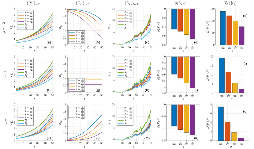
Figure 1: Experiment results: Optimal decision $\{P^{*}_{1}(t)\}_{t\in\mathcal{T}}$, investment opinion $\{Z_{1}(t)\}_{t\in\mathcal{T}}$, wealth $\{X_{1}(t)\}_{t\in\mathcal{T}}$, utility of terminal wealth $\phi(X_{1}(T))$, and average deviation $\mathscr{D}[P_{1}\|\bar{P}_{2}]$ with different decay rate $\rho$.

V-A Data Description and Parameter Settings

We choose a temporal span covering fifty years from Jan. 1972 to Dec. 2022, i.e., $T=50$. During this investment period, we gather daily closing prices of the Dow Jones Industrial Average as the daily prices for the risky asset. Utilizing parameter estimation of the geometric Brownian motion, we determined the expected return $\mu$ to be $0.07$ and volatility $\sigma$ to be $0.17$ for the risky asset. As the risk-free interest rate $r$, we selecte a reasonable value from the interest rates of Treasury Bills, setting it at $0.04$. According to the estimation of the risk aversion coefficient in [36], we choose $\alpha_{1}=0.2$, $\alpha_{2}=0.4$. Additionally, we set the modified herd coefficient $\vartheta$ to values of $\frac{1}{800}$, $\frac{1}{400}$, $\frac{1}{200}$, and $\frac{1}{100}$.

V-B Optimal Decision

In the experiments, we select three cases with different decay rates: $\rho=0$, $\rho=2$, and $\rho=4$. We assume that the initial wealth is zero, and the results for the case of positive initial wealth are analogous. Experimental results for A1’s optimal decision, investment opinion, wealth, utility of terminal wealth, and average deviation are illustrated in Fig. 1. Additionally, we include rational decision and its corresponding rational wealth curves in the optimal decision and wealth plots.

It is evident that A1’s optimal decision consistently remains within the region bounded by the rational decisions of the two agents. Moreover, with an increase in the herd coefficient, the optimal decision progressively approaches A2’s rational decision. When $\rho=0$, the investment opinion decreases over time (Fig. 1b), and the optimal decision increasingly converges towards A2’s rational decision (Fig. 1a), and the wealth also progressively approaches A2’s rational wealth (Fig. 1c). For $\rho=2$, the investment opinion remains constant (Fig. 1g), and the optimal decision maintains a constant distance from the rational decisions of the two agents (Fig. 1f), and the wealth similarly maintains a constant distance from the rational wealth of the two agents (Fig. 1h). In the case of $\rho=4$, the investment opinion increases over time (Fig. 1l), and the optimal decision increasingly converges towards A1’s own rational decision (Fig. 1k), and the wealth also progressively approaches A1’s own rational wealth (Fig. 1m). From Fig. 1d, 1i, 1n and 1e, 1j, 1o, it can be observed that with an increase in the herd coefficient, the utility of terminal wealth gradually decreases, and average deviation also diminishes.

V-C Investment Opinion

In keeping other parameters constant and ensuring $\frac{\alpha_{1}}{\alpha_{2}}\in\left[1-\frac{\sqrt{3}}{3},1+\frac{\sqrt{3}}{3}\right]$, we plot the curves of the integral constant $\eta$ with respect to the herd coefficient $\theta$, initial wealth $x$, excess return rate $\mu$, and volatility $\sigma$, as depicted in Fig. 2. It can be observed that $\eta$ increases with the decrease of $x$ and $v$, and increases with the increase of $\theta$ and $\sigma$, thereby confirming the correctness of Theorem 6.

Utilizing the relationship between the investment opinion function and the integral constant given by (12), we can also verify the correctness of Theorem 7. It is noteworthy that the relationship between the investment opinion function and the herd coefficient can be discerned from Fig. 1b, 1g, and 1l, indicating a decrease in the investment opinion function with an increase in the herd coefficient.

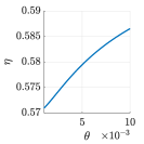
(a) Herd coefficient $\theta$

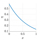
(b) Initial wealth $x$

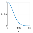
(c) Excess return rate $v$

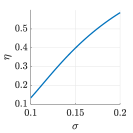
(d) Volatility $\sigma$

Figure 2: Experiment results: Parameter influence on the integral constant $\eta$.

VI Conclusion

This paper studies a dual-agent optimal investment problem that considers herd behavior based on the Merton problem. We obtain the analytical solution for this stochastic optimal control problem using the variational method and quantitatively analyze the impact of herd behavior on optimal decision-making through the rational decision decomposition approach. Additionally, we introduce the concept of an agent’s investment opinion to describe their preference for a rational decision over that of the other agent. There are several further problems that can be considered, of which we mention two: the stochastic differential game problem where two agents influence each other, as well as the macro problem where the number of the agents is sufficiently large.

References

• [1] A. Bodnaruk and A. Simonov, “Do financial experts make better investment decisions?” Journal of Financial Intermediation, vol. 24, no. 4, pp. 514–536, 2015.
• [2] H. Hong, J. D. Kubik, and J. C. Stein, “Social interaction and stock-market participation,” The Journal of Finance, vol. 59, no. 1, pp. 137–163, 2004.
• [3] J. R. Brown, Z. Ivković, P. A. Smith, and S. Weisbenner, “Neighbors matter: Causal community effects and stock market participation,” The Journal of Finance, vol. 63, no. 3, pp. 1509–1531, 2008.
• [4] S. Bikhchandani and S. Sharma, “Herd behavior in financial markets,” IMF Staff papers, vol. 47, no. 3, pp. 279–310, 2000.
• [5] R. Cont and J.-P. Bouchaud, “Herd behavior and aggregate fluctuations in financial markets,” Macroeconomic dynamics, vol. 4, no. 2, pp. 170–196, 2000.
• [6] V. M. Eguiluz and M. G. Zimmermann, “Transmission of information and herd behavior: An application to financial markets,” Physical review letters, vol. 85, no. 26, p. 5659, 2000.
• [7] D. Hirshleifer and S. Hong Teoh, “Herd behaviour and cascading in capital markets: A review and synthesis,” European Financial Management, vol. 9, no. 1, pp. 25–66, 2003.
• [8] S. Alfarano, T. Lux, and F. Wagner, “Estimation of agent-based models: The case of an asymmetric herding model,” Computational Economics, vol. 26, pp. 19–49, 2005.
• [9] E. C. Chang, J. W. Cheng, and A. Khorana, “An examination of herd behavior in equity markets: An international perspective,” Journal of Banking & Finance, vol. 24, no. 10, pp. 1651–1679, 2000.
• [10] M. Al-Shboul, “Asymmetric effects and the herd behavior in the Australian equity market,” International Journal of Business and Management, vol. 7, no. 7, p. 121, 2012.
• [11] T. T.-L. Chong, X. Liu, and C. Zhu, “What explains herd behavior in the Chinese stock market?” Journal of Behavioral Finance, vol. 18, no. 4, pp. 448–456, 2017.
• [12] H. Litimi, “Herd behavior in the French stock market,” Review of Accounting and Finance, 2017.
• [13] M. U. D. Shah, A. Shah, and S. U. Khan, “Herding behavior in the Pakistan stock exchange: Some new insights,” Research in International Business and Finance, vol. 42, pp. 865–873, 2017.
• [14] P. Wanidwaranan and C. Padungsaksawasdi, “Unintentional herd behavior via the Google search volume index in international equity markets,” Journal of International Financial Markets, Institutions and Money, vol. 77, p. 101503, 2022.
• [15] S. Zhou and X. Liu, “Internet postings and investor herd behavior: evidence from China’s open-end fund market,” Humanities and Social Sciences Communications, vol. 9, no. 1, pp. 1–11, 2022.
• [16] H. M. Markowitz, “Portfolio selection,” The Journal of Finance, vol. 7, no. 1, p. 77, 1952.
• [17] P. A. Samuelson, “Lifetime portfolio selection by dynamic stochastic programming,” Stochastic optimization models in finance, pp. 517–524, 1975.
• [18] G. C. Calafiore, “Multi-period portfolio optimization with linear control policies,” Automatica, vol. 44, no. 10, pp. 2463–2473, 2008.
• [19] L. Yang, Y. Zheng, and J. Shi, “Risk-sensitive stochastic control with applications to an optimal investment problem under correlated noises,” in 2019 Chinese Control Conference (CCC).   IEEE, 2019, pp. 1356–1363.
• [20] G. Li, Z. Huang, and Z. Wu, “A kind of optimal investment problem under inflation and uncertain exit time,” in 2022 41st Chinese Control Conference (CCC).   IEEE, 2022, pp. 1739–1744.
• [21] A. Aljalal and B. Gashi, “Optimal investment in a market with random interest rate for borrowing: an explicit closed-form solution,” in 2022 8th International Conference on Control, Decision and Information Technologies (CoDIT), vol. 1.   IEEE, 2022, pp. 764–769.
• [22] N. Alasmi and B. Gashi, “Optimal investment in a market with borrowing and a combined interest rate model,” in 2023 9th International Conference on Control, Decision and Information Technologies (CoDIT).   IEEE, 2023, pp. 01–06.
• [23] R. C. Merton, “Lifetime portfolio selection under uncertainty: The continuous-time case,” The Review of Economics and Statistics, pp. 247–257, 1969.
• [24] ——, “Optimum consumption and portfolio rules in a continuous-time model,” in Stochastic optimization models in finance.   Elsevier, 1975, pp. 621–661.
• [25] L. C. Rogers, Optimal investment.   Springer, 2013, vol. 1007.
• [26] J. Gali, “Keeping up with the Joneses: Consumption externalities, portfolio choice, and asset prices,” Journal of Money, Credit and Banking, vol. 26, no. 1, pp. 1–8, 1994.
• [27] C. Gollier, “Misery loves company: Equilibrium portfolios with heterogeneous consumption externalities,” International Economic Review, vol. 45, no. 4, pp. 1169–1192, 2004.
• [28] B. Lauterbach and H. Reisman, “Keeping up with the Joneses and the home bias,” European Financial Management, vol. 10, no. 2, pp. 225–234, 2004.
• [29] J.-P. Gómez, “The impact of keeping up with the Joneses behavior on asset prices and portfolio choice,” Finance Research Letters, vol. 4, no. 2, pp. 95–103, 2007.
• [30] J.-p. Gómez, R. Priestley, and F. Zapatero, “Implications of keeping-up-with-the-Joneses behavior for the equilibrium cross section of stock returns: International evidence,” The Journal of Finance, vol. 64, no. 6, pp. 2703–2737, 2009.
• [31] N. Roussanov, “Diversification and its discontents: Idiosyncratic and entrepreneurial risk in the quest for social status,” The Journal of Finance, vol. 65, no. 5, pp. 1755–1788, 2010.
• [32] D. Garcia and G. Strobl, “Relative wealth concerns and complementarities in information acquisition,” The Review of Financial Studies, vol. 24, no. 1, pp. 169–207, 2011.
• [33] M. Levy and H. Levy, “Keeping up with the Joneses and optimal diversification,” Journal of Banking & Finance, vol. 58, pp. 29–38, 2015.
• [34] J. M. Merigo and M. Casanovas, “Induced aggregation operators in the euclidean distance and its application in financial decision making,” Expert systems with applications, vol. 38, no. 6, pp. 7603–7608, 2011.
• [35] K. C. Border, Fixed point theorems with applications to economics and game theory.   Cambridge university press, 1985.
• [36] K. Yuen, H. Yang, and K. Chu, “Estimation in the constant elasticity of variance model,” British Actuarial Journal, vol. 7, no. 2, pp. 275–292, 2001.