Abstract

Recent advances in applying thermodynamic ideas to quantum systems have raised the novel prospect of using non-thermal, non-classical sources of energy, of purely quantum origin, like quantum statistics, to extract mechanical work in macroscopic quantum systems like Bose-Einstein condensates. On the other hand, thermodynamic ideas have also been applied to small systems like single molecules and quantum dots. In this paper we study the quantum thermodynamics of small systems of anyons, with specific emphasis on the quantum Otto engine which uses, as its working medium, just one or two anyons. Formulae are derived for the efficiency of the Otto engine as a function of the statistics parameter.

1 Introduction

Thermodynamics is an empirical and phenomenological description of matter at the macroscopic level, where the number of particles in the system is of the order of the Avogadro number [1]. It is of academic interest to stretch the thermodynamic line of thinking to small systems in order to probe the limits of applicability of concepts like temperature and entropy [2]. In the last few decades, several small systems, like single molecules and quantum dots, have been studied extensively from a thermodynamic point of view [3]. These studies are made possible by bringing the ideas of quantum mechanics and thermodynamics under one umbrella, with the obvious name of quantum thermodynamics, which allows us to push the frontiers of thermodynamics to the microscopic level.

When two disparate approaches to physical problems face off, as in the above case, surprises are to be expected. Classical thermodynamic engines like the Otto engine, studied and used for over a century, convert thermal energy to work. On the other hand, quantum thermodynamic engines afford us an opportunity to harness non-classical, non-thermal sources of energy, arising out of quantum statistics, to do mechanical work.

A simple back-of-the-envelope calculation reveals that for a harmonically trapped quantum bose gas of $N$ particles, the energy at zero temperature is $E^{B}=N\hbar\omega/2$ since all the particles occupy the ground state, whereas, for a fermi gas, for which all levels upto the Fermi energy $E_{Fermi}=\hbar\omega(2N-1)/2$, are occupied, it is $E^{F}=\hbar\omega N^{2}/2$. The difference in these energies, $E_{P}=E^{F}-E^{B}=\hbar\omega N(N-1)/2$, with its origin in the exclusion principle, and hence called the Pauli energy, can, in principle, be tapped by a quantum engine, and can be very large for large values of $N$, i.e. for macroscopic systems. This energy is non-classical, and purely quantum mechanical in origin, derived as it is from the quantum statistical population distribution functions of indistinguishable particles.

A recent paper by Koch et al [4] reports an experimental realization of the above idea by constructing a many-body quantum engine, fittingly called the Pauli engine, with harmonically trapped $~{}^{6}$Li atoms close to a magnetic Feshbach resonance. Like the classical Otto engine, the Pauli engine consists of four strokes viz. compression, fermionization, expansion, and bosonization. The change in quantum statistics of the gas is accomplished by tuning the magnetic field to drive the quantum gas back and forth between a Bose-Einstein condensate and a unitary Fermi gas, through the well-known phenomenon of BEC-BCS crossover [5].

In this, the first of two papers on the topic, we study the quantum thermodynamics of small systems, consisting of one or two anyons, to be precise, whose quantum statistics can be made to smoothly interpolate between the bosonic and fermionic limits, and construct an Otto engine which converts a change of quantum statistics to mechanical work in one dimension.

In section 2, we briefly review the formalism of quantum thermodynamics, with particular emphasis on the difference between a classical and quantum Otto engine. In section 3, we define the basic model of a quantum Otto engine based on anyons. In section 4, we advance a charged particle constrained to move on a ring threaded by a magnetic flux, as a model of a one-dimensional anyon. In section 5, we derive analogous results for two anyons on a ring in the Calogero-Sutherland model. For both the models we set up the quantum Otto engine and calculate its efficiency. We conclude with a few closing remarks in section 6.

2 Quantum Thermodynamics

The main idea of quantum thermodynamics is to identify the non-classical equivalents of thermodynamic concepts like internal energy, heat, and work in a quantum system [6].

Let $\rho$ be a density operator that describes a quantum system coupled to a thermal environment. Let $H(\lambda)$ be the system Hamiltonian, and $\lambda$ be a control parameter. The internal energy is defined by

$$E=~{}<H>~{}=~{}{\hbox{tr}}\{\rho H\}$$ (1)

where, in the weak coupling limit, $\rho$ is the equilibrium state of the system which we take to be the Gibbs’ state

$$\rho={1\over Z}{\hbox{exp}}(-\beta H)$$ (2)

where $Z={\hbox{tr}}~{}{\hbox{exp}}(-\beta H)$ is the partition function, with $\beta=1/k_{B}T$ as usual. As is well-known, the entropy for a Gibbs’ state is given by $S=-k_{B}~{}{\hbox{tr}}~{}\{\rho{\hbox{ln}}\rho\}$.

The change in internal energy can be partitioned into two pieces viz.

$$dE={\hbox{tr}}\{d\rho~{}H\}+{\hbox{tr}}\{\rho~{}dH\}=d\bar{}\hskip 10.00002ptQ+d\bar{}\hskip 10.00002ptW$$ (3)

The first term represents a change in entropy while the second term represents a change in the Hamiltonian, the $d\bar{}\hskip 10.00002pt$ indicating that neither of these changes is exact. In complete analogy with classical thermodynamics, we conclude that the work done corresponds to a displacement in the energy levels, and heat corresponds to a change in the probability distribution that populates the energy levels.

It is now straightforward to define quantum analogues of isothermal, isobaric, isochoric, and adiabatic processes, and hence the various quantum analogues of the classical thermodynamic engines.

The Otto engine, for example, consists of four strokes: two adiabats and two isochores. By definition, an adiabatic process is one in which no heat transfer takes place between the system and the environment and this corresponds to a change in the energy eigenvalues while keeping the populations, and hence the von Neumann entropy, unchanged. An isochoric process, on the other hand, keeps the energy eigenvalues fixed while allowing for changes in the populations of these levels.

To conclude this brief survey of quantum thermodynamics, we need to mention a few subtle points in which the classical and quantum versions of thermodynamics differ.

A classical adiabatic process is characterised by complete thermal insulation because of which no heat can be exchanged with the environment. A quantum adiabat on the other hand follows the adiabatic theorem in which the relevant eigenstate is dragged through the process. It is not possible to maintain a quantum adiabat for a long time because of decoherence. Thus, the time-scale of the adiabat should be less than the decoherence time-scale.

Unlike classical thermodynamical engines which are reversible, and are in instantaneous equilibrium through out, in quantum thermodynamic engines, finite-time adiabats drive the system out of equilibrium, and a relaxation process is necessary for a new equilibrium state to be reached through thermalization with a bath.

Quantum Otto engines based on qubits, three-level systems, harmonic oscillators, and statistical anyons [7] have been extensively studied. In this paper we study the quantum Otto engine with a working medium being a very small number of one-dimensional anyons – particles which intrinsically have any quantum statistics, and which can smoothly interpolate between the bosonic and fermionic limits.

3 An Anyonic Quantum Otto Process

As is well-known, the spin and statistics theorem in quantum theory allows for two types of particles: a) bosons, which have integer spin, have wavefunctions which transform under the symmetric representation of the permutation group, and follow the Bose-Einstein statistical distribution, and b) fermions, which have half-odd integer spin, have wavefunctions which transform under the alternating representation of the permutation group, and follow the Fermi-Dirac distribution [8].

In low dimensions, spin and statistics can take arbitrary values, and particles with such properties are called anyons. The underlying topological reasons for these more general possibilities have been extensively studied in two dimensions [9]. On a real line, an exchange of two indistinguishable particles requires us to take one particle through the other, and thus gets inextricably linked with interaction. This very fact allows us to define exchange statistics. In the next couple of sections, we consider two such models. The first is that of a charged particle constrained to move on a circular ring threaded by a magnetic flux which influences the periodicity properties of the particle’s wavefunction [10]. The second realises anyonic statistics through an interaction between two particles as described by the Calogero-Sutherland Hamiltonian [11].

4 Charged Particle On A Ring Threaded By A Magnetic Flux Tube

In this example, we have an infinitely long solenoid of cross-sectional area $A$, carrying a magnetic field $(0,0,B)$. The magnetic flux is $\Phi=BA$.

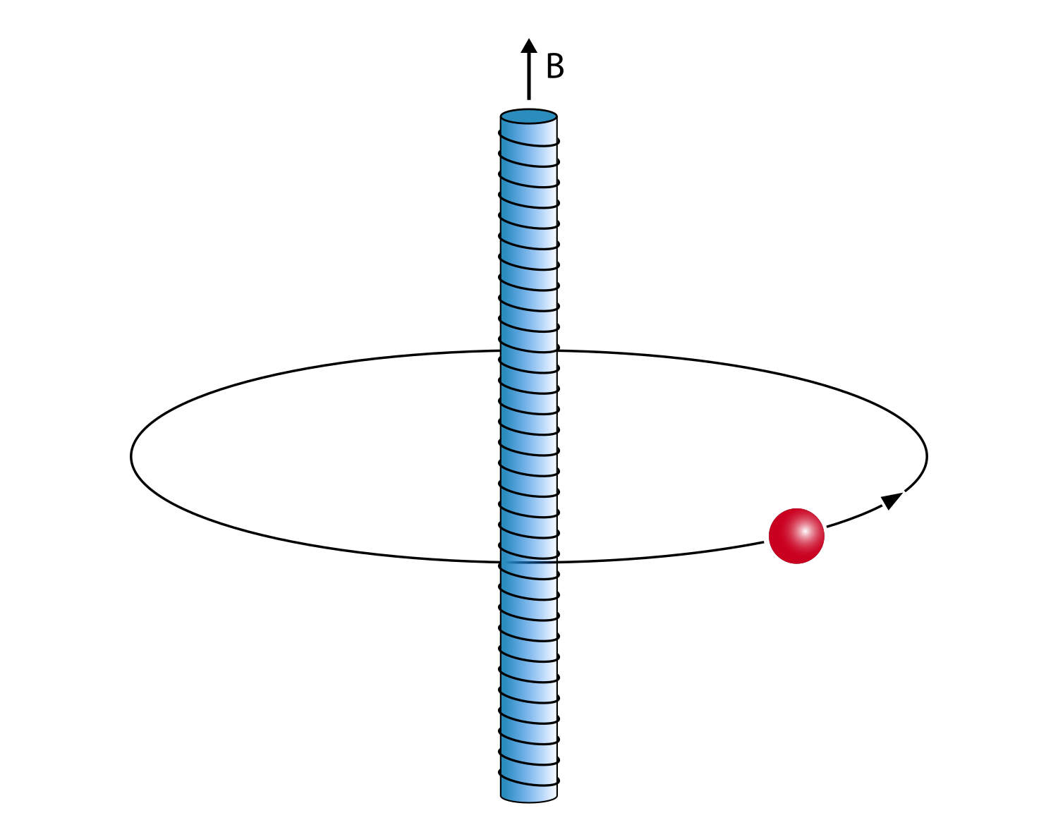
Figure 1: Charge Circling A Magnetic Flux Tube

Although it doesn’t make sense to talk about statistics of individual particles, this may be considered as a toy model of an anyon on a ring of radius $a$. To verify this statement all we have to do is to consider two particles on the ring and exchange their positions.

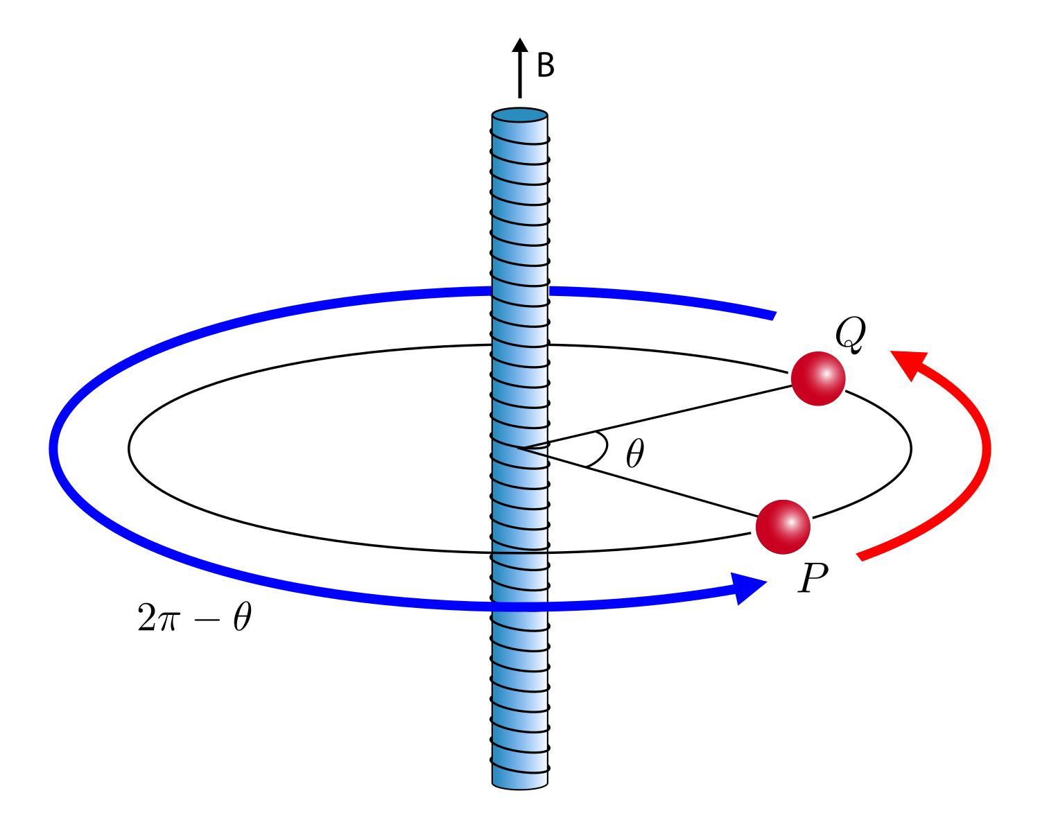
Figure 2: Two Anyons On A Ring

As already mentioned, it is not possible to exchange particle positions in one dimensional space ($R^{1}$) without taking them through each other. However, as can be seen from the figure, this problem can be bypassed for two particles on a ring. The two-particle wavefunction thus picks up an Aharonov-Bohm phase ${\hbox{exp}}~{}[2i\pi\Phi]$ under an exchange, which may be interpreted as the phase factor acquired in exchanging anyons.

The vector potential has only the azimuthal component

$$\begin{aligned} A_{\phi}=\frac{\Phi}{2\pi r}\end{aligned}$$ (4)

The Hamiltonian of a charged particle $q$ on the ring is

$$\begin{aligned} H=\frac{1}{2m}\left(p_{\phi}-qA_{\phi}\right)^{2}=\frac{1}{2ma^{2}}\left(-i\hbar\frac{\partial}{\partial\phi}-\frac{q\Phi}{2\pi}\right)^{2}\end{aligned}$$ (5)

The normalised energy eigenstates are

$$\begin{aligned} \psi_{n}(\phi)=\frac{1}{\sqrt{2\pi}}e^{in\phi},~{}~{}n\in\mathbb{Z}\end{aligned}$$ (6)

with energy eigenvalues

$$\begin{aligned} E_{n}=\frac{\hbar^{2}}{2ma^{2}}\left(n-\alpha\right)^{2},~{}~{}~{}\alpha=\frac{q\Phi}{2\pi\hbar}\end{aligned}$$ (7)

4.1 Quantum Otto Engine

A schematic diagram of the quantum Otto engine is given below.

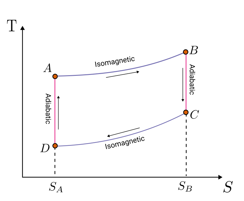
Figure 3: The Quantum Otto Engine

The four strokes that constitute the quantum Otto engine are as follows: In the first step, as we move from $A$ to $B$, the system changes its temperature from $T_{l}$ to $T_{h}$. This is achieved by bringing the system in contact with an infinite bath at each infinitesimal temperature step as $T_{l}\rightarrow T_{l}+\Delta T\rightarrow T_{l}+2\Delta T,\cdots\rightarrow T_{l}+(N-1)\Delta T\rightarrow T_{l}+N\Delta T=T_{h}$. As $\Delta T\rightarrow 0,~{}N\rightarrow\infty$, such that $N\Delta T=T_{h}-T_{l}$, we get a reversible path. This is because the entropy change of the reservoir and the system is zero at each stage. Similar arguments hold for the path $C$ to $D$.

$A\to B$ and $C\to D$ are isomagnetic processes, thus called because no work is done along these paths. Recall that changes in energy levels (quantum work) are effected by changes in the magnetic field. The strength of the magnetic field on $A\to B$ is chosen to be $B_{h}$, and correspondingly, the energy is $E_{n}^{h}=\frac{\hbar^{2}}{2ma^{2}}\left(n-\alpha_{h}\right)^{2}$, where $\alpha_{h}=\pi a^{2}B_{h}$. Similarly, from $C\to D$ the energy levels are $E_{n}^{l}=\frac{\hbar^{2}}{2ma^{2}}\left(n-\alpha_{l}\right)^{2}$ and the corresponding magnetic field is $B_{l}$. The change in the magnetic field along the adiabats produces a current which can be translated to mechanical work.

Alternatively, we can keep the magnetic field constant and change the radius of the ring, i.e. along $AB$ and $CD$, the energy levels are given by $E^{h}_{n}={\hbar^{2}\over ma_{1}^{2}}(n-\pi a_{1}^{2}B)$ and $E^{l}_{n}={\hbar^{2}\over ma_{2}^{2}}(n-\pi a_{2}^{2}B)$ respectively.

If $a_{2}>a_{1}$, $E_{n}$ decreases, i.e. $E_{n}^{h}>E_{n}^{l}$, but since the occupation probabilities $P_{n}$ remain the same in the adiabatic processes $B\to C$ and $D\to A$, work is done by the system as we go from $B$ to $C$, and on the system as we go from $D$ to $A$. In both cases, the entropy remains the same. Note that only the states $B$ and $D$ are in thermal equilibrium, but not $A$ and $C$.

The efficiency of the quantum Otto cycle is give by

$$\begin{aligned} \eta_{QOE}=\frac{W_{out}}{Q_{in}}=1-\frac{\sum_{n}E^{l}_{n}(P_{n}(B)-P_{n}(A))}{\sum_{m}E^{h}_{m}(P_{m}(B)-P_{m}(A))}\end{aligned}$$ (8)

where $P_{n}(X)=\frac{e^{-\beta_{X}E_{n}(X)}}{Z(X)}$. It is easy to check that each term in the summand in the numerator is less than the corresponding term in the denominator since $P_{n}(B)-P_{n}(A)>0$ as we move from lower to higher temperature, and $E_{n}^{l}<E_{n}^{h}$ for $a_{1}<a_{2}$ consistent with $1>\eta>0$. Using the expressions

$$\begin{aligned} P_{n}(B)=P_{n}(C)&=\frac{e^{-\beta_{h}E^{h}_{n}}}{\sum_{n}e^{-\beta_{h}E^{h}_{n}}}\\ P_{n}(A)=P_{n}(D)&=\frac{e^{-\beta_{l}E^{l}_{n}}}{\sum_{n}e^{-\beta_{l}E^{l}_{n}}}\\ \end{aligned}$$ (9)

we write

$$\begin{aligned} \eta&=1-\frac{\left(\frac{\sum_{n}E^{l}_{n}e^{-\beta_{h}E^{h}_{n}}}{\sum_{n_{1}}e^{-\beta_{h}E^{h}_{n_{1}}}}-\frac{\sum_{n}E^{l}_{n}e^{-\beta_{l}E^{l}_{n}}}{\sum_{n_{2}}e^{-\beta_{l}E^{l}_{n_{2}}}}\right)}{\left(\frac{\sum_{n}E^{h}_{m}e^{-\beta_{h}E^{h}_{m}}}{\sum_{m_{1}}e^{-\beta_{h}E^{h}_{m_{1}}}}-\frac{\sum_{n}E^{h}_{m}e^{-\beta_{l}E^{l}_{m}}}{\sum_{m_{2}}e^{-\beta_{l}E^{l}_{m_{2}}}}\right)}\end{aligned}$$ (10)

The sums appearing in the above equation can be calculated in a straighforward manner, and give the following analytic expression for the efficiency of the anyonic quantum Otto engine:

$$\begin{aligned} \eta&=1-\frac{\frac{\Upsilon(l,h)}{Z_{h}}-\frac{\Upsilon(l,l)}{Z_{l}}}{\frac{\Upsilon(h,h)}{Z_{h}}-\frac{\Upsilon(h,l)}{Z_{l}}}\end{aligned}$$ (11)

where

$$\begin{aligned} \Upsilon(k,j)&=\sum_{n=-\infty}^{\infty}E^{k}_{n}e^{-\beta_{j}E^{j}_{n}},~{}~{}~{}~{}j,k=h,l\\ &=\sum_{n=-\infty}^{\infty}\frac{\hbar^{2}}{2ma^{2}}\left(n-\alpha_{k}\right)^{2}e^{-\beta_{j}\frac{\hbar^{2}}{2ma^{2}}\left(n-\alpha_{j}\right)^{2}}\\ &=\frac{\hbar^{2}}{2ma^{2}}\bigg{(}c^{2}e^{-\lambda\gamma^{2}}\vartheta_{3}\left(e^{2\lambda\gamma},e^{-\lambda}\right)+e^{-\lambda\gamma^{2}}\frac{(c\gamma)}{\lambda}\frac{\partial}{\partial\gamma}\vartheta_{3}\left(e^{2\lambda\gamma},e^{-\lambda}\right)\\ &-e^{-\lambda\gamma^{2}}\frac{\partial}{\partial\lambda}\vartheta_{3}\left(e^{2\lambda\gamma},e^{-\lambda}\right)\bigg{)}\bigg{|}_{c=\alpha_{k},\lambda=\beta_{j}\frac{\hbar^{2}}{2ma^{2}},\gamma=\alpha_{j}}\end{aligned}$$ (12)

and the partition function is given by

$$\begin{aligned} Z_{j}&=\sum_{n=-\infty}^{\infty}e^{-\beta_{j}E^{j}_{n}},~{}~{}j=h,l\\ &=\sum_{n=-\infty}^{\infty}e^{-\beta_{j}\frac{\hbar^{2}}{2ma^{2}}\left(n-\alpha_{j}\right)^{2}}\\ &=e^{-\beta_{j}\frac{\hbar^{2}}{2ma^{2}}\alpha_{j}^{2}}\vartheta_{3}\left(\frac{\alpha_{j}\beta_{j}\hbar^{2}}{2ma^{2}},e^{-\beta_{j}\frac{\hbar^{2}}{2ma^{2}}}\right)\end{aligned}$$ (13)

The Jacobi theta function $\vartheta_{3}\left(x,q\right)$ in terms of which the above expressions are written, is defined by

$$\begin{aligned} \vartheta_{3}\left(x,q\right)&=\sum_{n=-\infty}^{\infty}q^{n^{2}}x^{n}\end{aligned}$$ (14)

The detailed calculations of the above results are relegated to the Appendix.

5 Two Anyons On A One-Dimensional Ring

Consider a system of two particles on a ring of finite circumference ($2\pi L$) with periodic boundary conditions [11]. The Hamiltonian of the system is

$$\begin{aligned} H=-\frac{\hbar^{2}}{2m}\sum_{j}\frac{\partial^{2}}{\partial x_{j}^{2}}+\frac{\pi^{2}\alpha(\alpha-1)}{L^{2}}\sum_{j<k}\frac{1}{\sin^{2}\left(\frac{\pi(x_{j}-x_{k})}{L^{2}}\right)}\end{aligned}$$ (15)

In this case, the magnetic field of the previous section is replaced by an interaction between the two particles, with the strength of the interaction being directly related to the quantum statistics of the two particles.

Setting $\hbar=m=1$ to avoid clutter, the energy levels of the two-particle system are

$$\begin{aligned} E_{n_{1},n_{2}}(L)=\frac{\pi^{2}\alpha^{2}}{L^{2}}+\frac{2\pi^{2}}{L^{2}}\left(n_{1}^{2}+n_{2}^{2}+\alpha(n_{1}-n_{2})\right)\end{aligned}$$ (16)

where $n_{1},n_{2}$ are integers, $n_{1}\leq n_{2}$. The corresponding energy eigenstates are:

$$\psi(\theta)=\Phi(\theta)\Delta^{\alpha}(\theta)$$ (17)

with $\Phi$ being a symmetric polynomial in the variables $z_{i}=e^{i\theta_{j}}$ and $z_{j}^{-1}$, $\theta$ being related to the coordinates by the equation $\theta_{j}=2\pi x_{j}/L$, and the Jastrow factor being

$$\Delta(\theta)=\prod_{i<j}{\hbox{sin}}({\theta_{i}-\theta_{j}\over 2})$$ (18)

The antisymmetry of $\Delta$ implies, in particular, that $\alpha=0$ and $\alpha=1$ correspond to bosons and fermions respectively. For other intermediate values, the particles have anyonic statistics.

5.1 The Quantum Otto Engine

The two volumes can be chosen as $V_{1}=L_{1}$ and $V_{2}=L_{2}$. The inverse temperature of the hot reservoir is $\beta_{h}$ and that of the cold reservoir is $\beta_{l}$. Energy levels are labeled by $(n_{1},n_{2})$ where $n_{1}\leq n_{2}$.

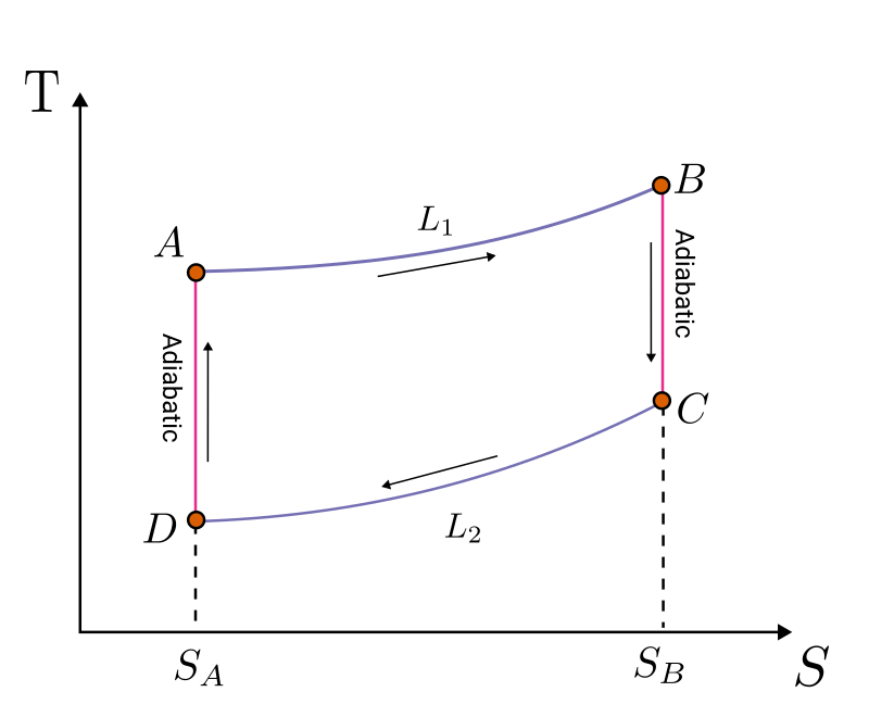
Figure 4: The Quantum Otto Engine: variable volume, fixed coupling

We have

$$\begin{aligned} E_{n_{1},n_{2}}(L_{1})&=\frac{\pi^{2}\alpha^{2}}{L_{1}^{2}}+\frac{2\pi^{2}}{L_{1}^{2}}\left(n_{1}^{2}+n_{2}^{2}+\alpha(n_{1}-n_{2})\right)\\ E_{n_{1},n_{2}}(L_{2})&=\frac{\pi^{2}\alpha^{2}}{L_{2}^{2}}+\frac{2\pi^{2}}{L_{2}^{2}}\left(n_{1}^{2}+n_{2}^{2}+\alpha(n_{1}-n_{2})\right)\\ P_{n_{1},n_{2}}(B)&=\frac{e^{-\beta_{h}E_{n_{1},n_{2}}(L_{1})}}{\sum_{n_{1}\leq n_{2}}e^{-\beta_{h}E_{n_{1},n_{2}}(L_{1})}}\\ P_{n_{1},n_{2}}(A)&=\frac{e^{-\beta_{l}E_{n_{1},n_{2}}(L_{2})}}{\sum_{n_{1}\leq n_{2}}e^{-\beta_{l}E_{n_{1},n_{2}}(L_{2})}}\\ \end{aligned}$$ (19)

All the steps mentioned in Section 4, for the case of a single anyon, can be repeated in exactly the same manner. The efficiency of the quantum Otto engine is then

$$\begin{aligned} \eta_{QOE}=\frac{W_{out}}{Q_{in}}=1-\frac{\sum_{n_{1}\leq n_{2}}E_{n_{1},n_{2}}(L_{1})(P_{n_{1},n_{2}}(B)-P_{n_{1},n_{2}}(A))}{\sum_{m_{1}\leq m_{2}}E_{m_{1},m_{2}}(L_{2})(P_{m_{1},m_{2}}(B)-P_{m_{1},m_{2}}(A))}\end{aligned}$$ (20)

Since $E_{n_{1},n_{2}}(L)\propto\frac{1}{L^{2}}$, we have

$$\begin{aligned} E_{n_{1},n_{2}}(L_{1})=\frac{L_{2}^{2}}{L_{1}^{2}}E_{n_{1},n_{2}}(L_{2})\end{aligned}$$ (21)

Therefore the efficiency is

$$\eta_{QOE} =1-L_{2}^{2}/L_{1}^{2}$$ (22)

It is interesting to note that, in this case, the result is essentially the the same as the classical result. This is a consequence of the fact that energy scales as the inverse square of the length in both cases.

However, the length $L$ is not the only parameter on which the energy levels depend. As already mentioned, the strength of the interaction $\alpha$ plays the same role as the magnetic field in the previous section, and is responsible for the quantum (anyonic) statistics of the particles. As can be seen from the expression for the energy spectrum, the dependence of the energy levels on $\alpha$ cannot be scaled away. We therefore define a quantum Otto engine in this case by the following diagram:

Figure 5: The Quantum Otto Engine: fixed volume, variable coupling

Once again with all the caveats delineated in the previous examples hold.

5.2 Efficiency as a function of the coupling (statistics parameter) $\alpha$

We are now in a position to compute the efficiency in terms of the statistics parameter $\alpha$, keeping $L$ fixed. The relevant formulae are

$$\begin{aligned} E_{n_{1},n_{2}}(\alpha_{1})&=\frac{\pi^{2}\alpha_{1}^{2}}{L^{2}}+\frac{2\pi^{2}}{L^{2}}\left(n_{1}^{2}+n_{2}^{2}+\alpha_{1}(n_{1}-n_{2})\right)\\ E_{n_{1},n_{2}}(\alpha_{2})&=\frac{\pi^{2}\alpha_{1}^{2}}{L^{2}}+\frac{2\pi^{2}}{L^{2}}\left(n_{1}^{2}+n_{2}^{2}+\alpha_{2}(n_{1}-n_{2})\right)\\ P_{n_{1},n_{2}}(B)&=P_{n_{1},n_{2}}(B)=\frac{e^{-\beta_{h}E_{n_{1},n_{2}}(\alpha_{1})}}{\sum_{n_{1}\leq n_{2}}e^{-\beta_{h}E_{n_{1},n_{2}}(\alpha_{1})}}\\ P_{n_{1},n_{2}}(A)&=\frac{e^{-\beta_{l}E_{n_{1},n_{2}}(\alpha_{2})}}{\sum_{n_{1}\leq n_{2}}e^{-\beta_{l}E_{n_{1},n_{2}}(\alpha_{2})}}\\ \end{aligned}$$ (23)

The efficiency of the quantum Otto engine can then be written as

$$\begin{aligned} \eta_{QOE}&=\frac{W_{out}}{Q_{in}}=1-\frac{\sum_{n_{1}\leq n_{2}}E_{n_{1},n_{2}}(\alpha_{1})(P_{n_{1},n_{2}}(B)-P_{n_{1},n_{2}}(A))}{\sum_{m_{1}\leq m_{2}}E_{m_{1},m_{2}}(\alpha_{2})(P_{m_{1},m_{2}}(B)-P_{m_{1},m_{2}}(A))}\\ \end{aligned}$$ (24)

To compute this efficiency, we will need to compute the partition function and the sums using theta and partial theta functions – an exercise we once again relegate to the Appendix. The result is given by

$$\begin{aligned} \eta&=\frac{W_{out}}{Q_{in}}=1-\frac{\sum_{n_{1}\leq n_{2}}E_{n_{1},n_{2}}(\alpha_{1})(P_{n_{1},n_{2}}(B)-P_{n_{1},n_{2}}(A))}{\sum_{m_{1}\leq m_{2}}E_{m_{1},m_{2}}(\alpha_{2})(P_{m_{1},m_{2}}(B)-P_{m_{1},m_{2}}(A))}\\ &=1-\frac{\frac{\mathcal{X}\left(\alpha_{1},\alpha_{1},\beta_{h}\right)}{Z\left(\alpha_{1},\beta_{h}\right)}-\frac{\mathcal{X}\left(\alpha_{1},\alpha_{2},\beta_{l}\right)}{Z\left(\alpha_{2},\beta_{1}\right)}}{\frac{\mathcal{X}\left(\alpha_{2},\alpha_{1},\beta_{h}\right)}{Z\left(\alpha_{1},\beta_{h}\right)}-\frac{\mathcal{X}\left(\alpha_{2},\alpha_{2},\beta_{l}\right)}{Z\left(\alpha_{2},\beta_{1}\right)}}\end{aligned}$$ (25)

where

$$\begin{aligned} \mathcal{X}\left(\alpha,\alpha^{\prime},\beta\right)&=\frac{4\pi^{2}}{L^{2}}\left(4\chi_{1}\left(-\frac{\pi^{2}\beta}{L^{2}},0,0\right)\chi_{2}\left(-\frac{4\pi^{2}\beta}{L^{2}},\alpha/2,\alpha^{\prime}/2\right)\right)\\ &+\frac{\pi^{2}}{L^{2}}\left(4\chi_{1}\left(-\frac{4\pi^{2}\beta}{L^{2}},-1/2,-1/2\right)\chi_{2}\left(-\frac{4\pi^{2}\beta}{L^{2}},(\alpha+1)/2,(\alpha^{\prime}+1)/2\right)\right)\end{aligned}$$ (26)

with

$$\begin{aligned} \chi_{1}\left(\lambda,\gamma,c\right)=&\sum_{n=-\infty}^{\infty}\left(n-c\right)^{2}e^{-\lambda(n-\gamma)^{2}}\\ =&c^{2}e^{-\lambda\gamma^{2}}\vartheta_{3}\left(e^{2\lambda\gamma},e^{-\lambda}\right)+e^{-\lambda\gamma^{2}}\frac{(\gamma-c)}{\lambda}\frac{\partial}{\partial\gamma}e^{-\lambda\gamma^{2}}\vartheta_{3}\left(e^{2\lambda\gamma},e^{-\lambda}\right)\\ &-e^{-\lambda\gamma^{2}}\frac{\partial}{\partial\lambda}e^{-\lambda\gamma^{2}}\vartheta_{3}\left(e^{2\lambda\gamma},e^{-\lambda}\right)\\ \end{aligned}$$ (27)

and

$$\begin{aligned} \chi_{2}\left(\lambda,\gamma,c\right)=&\sum_{n=0}^{\infty}\left(n-c\right)^{2}e^{-\lambda(n-\gamma)^{2}}\\ =&c^{2}e^{-\lambda\gamma^{2}}\Theta_{p}\left(e^{2\lambda\gamma},e^{-\lambda}\right)+e^{-\lambda\gamma^{2}}\frac{(\gamma-c)}{\lambda}\frac{\partial}{\partial\gamma}e^{-\lambda\gamma^{2}}\Theta_{p}\left(e^{2\lambda\gamma},e^{-\lambda}\right)\\ &-e^{-\lambda\gamma^{2}}\frac{\partial}{\partial\lambda}e^{-\lambda\gamma^{2}}\Theta_{p}\left(e^{2\lambda\gamma},e^{-\lambda}\right)\\ \end{aligned}$$ (28)

where

$$\begin{aligned} \vartheta_{3}\left(x,q\right)&=\sum_{n=-\infty}^{\infty}q^{n^{2}}x^{n}\\ \Theta_{p}(x,q)&=\sum_{n=0}^{\infty}q^{n^{2}}x^{n}\end{aligned}$$ (29)

define the Jacobi theta function, and the partial theta function respectively.

The efficiency is

$$\begin{aligned} \eta_{QOE}&=\frac{W_{out}O}{Q_{in}}=1-\frac{\sum_{n_{1}\leq n_{2}}E_{n_{1},n_{2}}(\alpha_{1})(P_{n_{1},n_{2}}(B)-P_{n_{1},n_{2}}(A))}{\sum_{m_{1}\leq m_{2}}E_{m_{1},m_{2}}(\alpha_{2})(P_{m_{1},m_{2}}(B)-P_{m_{1},m_{2}}(A))}\\ &=1-\frac{\frac{\mathcal{X}\left(\alpha_{1},\alpha_{1},\beta_{h}\right)}{Z\left(\alpha_{1},\beta_{h}\right)}-\frac{\mathcal{X}\left(\alpha_{1},\alpha_{2},\beta_{l}\right)}{Z\left(\alpha_{2},\beta_{1}\right)}}{\frac{\mathcal{X}\left(\alpha_{2},\alpha_{1},\beta_{h}\right)}{Z\left(\alpha_{1},\beta_{h}\right)}-\frac{\mathcal{X}\left(\alpha_{2},\alpha_{2},\beta_{l}\right)}{Z\left(\alpha_{2},\beta_{1}\right)}}\end{aligned}$$ (30)

Since $\alpha_{1}=0$ and $\alpha_{2}=1$, correspond to Bose and Fermi statistics respectively, by going through a thermodynamic cycle which changes the quantum statistics, we specialise to the case of an Otto engine based on Bose-Fermi transmutation, as in [4]. In general, $\alpha_{1}$ and $\alpha_{2}$ can take any real values.

6 Conclusions

In this paper, a detailed study of quantum thermodynamics of small systems is carried out in the specific context of the quantum Otto engine. The working medium is chosen to be one or two anyons in one dimension, whose quantum statistics interpolates between the bosonic and fermionic cases. Since we accomplish these results using a small number of anyons, we do not rely on the macroscopic BEC-BCS crossover studied in [4].

It would be interesting to generalise these results to other thermodynamic engines. It would also be interesting to choose two-dimensional anyons, and non-abelian anyons as the working medium. We will report the results of those cases in the near future.

7 Acknowledgements

This work is partially supported by a grant to CMI from the Infosys Foundation.

Appendix A Particle on a Ring Threaded by a Magnetic Field

We need to compute sums of the form

$$\begin{aligned} Z_{j}&=\sum_{n=-\infty}^{\infty}e^{-\beta_{j}E^{j}_{n}}\\ \Upsilon(k,j)&=\sum_{n=-\infty}^{\infty}E^{k}_{n}e^{-\beta_{j}E^{j}_{n}},~{}~{}j,k=h,l\\ \end{aligned}$$ (31)

The Jacobi theta function, defined by

$$\begin{aligned} \vartheta_{3}\left(x,q\right)&=\sum_{n=-\infty}^{\infty}q^{n^{2}}x^{n}\end{aligned}$$ (32)

may be used to compute the sums. Using this we have

$$\begin{aligned} \sum_{n=-\infty}^{\infty}e^{-\lambda(n-\gamma)^{2}}=&e^{-\lambda\gamma^{2}}\sum_{n=-\infty}^{\infty}e^{-\lambda n^{2}+2\lambda\gamma n}\\ &=e^{-\lambda\gamma^{2}}\vartheta_{3}\left(e^{2\lambda\gamma},e^{-\lambda}\right)\end{aligned}$$ (33)

$$\begin{aligned} \sum_{n=-\infty}^{\infty}ne^{-\lambda(n-\gamma)^{2}}&=e^{-\lambda\gamma^{2}}\frac{1}{2\lambda}\frac{\partial}{\partial\gamma}\sum_{n=-\infty}^{\infty}e^{-\lambda n^{2}+2\lambda\gamma n}\\ &=e^{-\lambda\gamma^{2}}\frac{1}{2\lambda}\frac{\partial}{\partial\gamma}\vartheta_{3}\left(e^{2\lambda\gamma},e^{-\lambda}\right)\end{aligned}$$ (34)

Also,

$$\begin{aligned} e^{-\lambda\gamma^{2}}\frac{\partial}{\partial\lambda}\vartheta_{3}\left(e^{2\lambda\gamma},e^{-\lambda}\right)&=\sum_{n=-\infty}^{\infty}\left(-n^{2}+2\gamma n\right)e^{-\lambda(n-\gamma)^{2}}\end{aligned}$$ (35)

From this

$$\begin{aligned} \sum_{n=-\infty}^{\infty}\left(n^{2}\right)e^{-\lambda(n-\gamma)^{2}}&=e^{-\lambda\gamma^{2}}\frac{\gamma}{\lambda}\frac{\partial}{\partial\gamma}\vartheta_{3}\left(e^{2\lambda\gamma},e^{-\lambda}\right)-e^{-\lambda\gamma^{2}}\frac{\partial}{\partial\lambda}e^{-\lambda\gamma^{2}}\vartheta_{3}\left(e^{2\lambda\gamma},e^{-\lambda}\right)\end{aligned}$$ (36)

Therefore

$$\begin{aligned} \sum_{n=-\infty}^{\infty}\left(n-c\right)^{2}e^{-\lambda(n-\gamma)^{2}}=&c^{2}e^{-\lambda\gamma^{2}}\vartheta_{3}\left(e^{2\lambda\gamma},e^{-\lambda}\right)+e^{-\lambda\gamma^{2}}\frac{c\gamma}{\lambda}\frac{\partial}{\partial\gamma}\vartheta_{3}\left(e^{2\lambda\gamma},e^{-\lambda}\right)\\ &-e^{-\lambda\gamma^{2}}\frac{\partial}{\partial\lambda}\vartheta_{3}\left(e^{2\lambda\gamma},e^{-\lambda}\right)\\ \end{aligned}$$ (37)

The partition function follows immediately:

$$\begin{aligned} Z_{j}&=\sum_{n=-\infty}^{\infty}e^{-\beta_{j}E^{j}_{n}},~{}~{}j=h,l\\ &=\sum_{n=-\infty}^{\infty}e^{-\beta_{j}\frac{\hbar^{2}}{2ma^{2}}\left(n-\alpha_{j}\right)^{2}}\\ &=e^{-\beta_{j}\frac{\hbar^{2}}{2ma^{2}}\alpha_{j}^{2}}\vartheta_{3}\left(\frac{\alpha_{j}\beta_{j}\hbar^{2}}{2ma^{2}},e^{-\beta_{j}\frac{\hbar^{2}}{2ma^{2}}}\right)\end{aligned}$$ (38)

with

$$\begin{aligned} \Upsilon(k,j)&=\sum_{n=-\infty}^{\infty}E^{k}_{n}e^{-\beta_{j}E^{j}_{n}},~{}~{}~{}~{}j,k=h,l\\ &=\sum_{n=-\infty}^{\infty}\frac{\hbar^{2}}{2ma^{2}}\left(n-\alpha_{k}\right)^{2}e^{-\beta_{j}\frac{\hbar^{2}}{2ma^{2}}\left(n-\alpha_{j}\right)^{2}}\\ &=\frac{\hbar^{2}}{2ma^{2}}\bigg{(}c^{2}e^{-\lambda\gamma^{2}}\vartheta_{3}\left(e^{2\lambda\gamma},e^{-\lambda}\right)+e^{-\lambda\gamma^{2}}\frac{(c\gamma)}{\lambda}\frac{\partial}{\partial\gamma}\vartheta_{3}\left(e^{2\lambda\gamma},e^{-\lambda}\right)\\ &-e^{-\lambda\gamma^{2}}\frac{\partial}{\partial\lambda}\vartheta_{3}\left(e^{2\lambda\gamma},e^{-\lambda}\right)\bigg{)}\bigg{|}_{c=\alpha_{k},\lambda=\beta_{j}\frac{\hbar^{2}}{2ma^{2}},\gamma=\alpha_{j}}\end{aligned}$$ (39)

The efficiency is

$$\begin{aligned} \eta&=1-\frac{\frac{\Upsilon(l,h)}{Z_{h}}-\frac{\Upsilon(l,l)}{Z_{l}}}{\frac{\Upsilon(h,h)}{Z_{h}}-\frac{\Upsilon(h,l)}{Z_{l}}}\end{aligned}$$ (40)

Appendix B Two-Anyons on a One-Dimensional Ring

The partition function is given by

$$\begin{aligned} Z(\alpha,\beta)&=\sum_{n_{1}\leq n_{2}}e^{-\beta E_{n_{1},n_{2}}(\alpha)}\\ &=\sum_{n_{1}\leq n_{2}}e^{-\beta\left(\frac{\pi^{2}\alpha^{2}}{L_{1}^{2}}+\frac{2\pi^{2}}{L_{1}^{2}}\left(n_{1}^{2}+n_{2}^{2}+\alpha(n_{1}-n_{2})\right)\right)}\\ &=e^{-\beta\left(\frac{\pi^{2}\alpha^{2}}{L_{1}^{2}}\right)}\sum_{n_{1}\leq n_{2}}e^{-\beta\left(\frac{2\pi^{2}}{L_{1}^{2}}\left(n_{1}^{2}+n_{2}^{2}+\alpha(n_{1}-n_{2})\right)\right)}\end{aligned}$$ (41)

We define $m=n_{1}+n_{2}$ and $n=n_{2}-n_{1}$. We then have

$$\begin{aligned} E_{n_{1},n_{2}}(\alpha)=E_{m,n}(\alpha_{1})=\frac{\pi^{2}}{L^{2}}\left(n^{2}+(m+\alpha)^{2}\right)\end{aligned}$$ (42)

This gives

$$\begin{aligned} Z(\alpha,\beta)&=\sum_{p_{1}=-\infty}^{\infty}\sum_{p_{2}=0}^{\infty}e^{-\beta\frac{\pi^{2}}{L^{2}}\left((2p_{1})^{2}+(2p_{2}+\alpha)^{2}\right)}+\sum_{p_{1}=-\infty}^{\infty}\sum_{p_{2}=0}^{\infty}e^{-\beta\frac{\pi^{2}}{L^{2}}\left((2p_{1}+1)^{2}+(2p_{2}+1+\alpha)^{2}\right)}\end{aligned}$$ (43)

The first term corresponds to both $n$ and $m$ even and the second term corresponds to both $n$ and $m$ odd. The Jacobi theta function and the partial theta function are given by

$$\begin{aligned} \vartheta_{3}\left(x,q\right)&=\sum_{n=-\infty}^{\infty}q^{n^{2}}x^{n}\\ \Theta_{p}(x,q)&=\sum_{n=0}^{\infty}q^{n^{2}}x^{n}\end{aligned}$$ (44)

Then,

$$\begin{aligned} Z(\alpha,\beta)&=\sum_{p_{1}=-\infty}^{\infty}\sum_{p_{2}=0}^{\infty}e^{-\beta\frac{\pi^{2}}{L^{2}}\left((2p_{1})^{2}+(2p_{2}+\alpha)^{2}\right)}+\sum_{p_{1}=-\infty}^{\infty}\sum_{p_{2}=0}^{\infty}e^{-\beta\frac{\pi^{2}}{L^{2}}\left((2p_{1}+1)^{2}+(2p_{2}+1+\alpha)^{2}\right)}\\ &=\sum_{p_{1}=-\infty}^{\infty}e^{-\beta\frac{4\pi^{2}}{L^{2}}p_{1}^{2}}\sum_{p_{2}=0}^{\infty}e^{-\beta\frac{\pi^{2}}{L^{2}}\left(4p_{2}^{2}+4p_{2}\alpha+\alpha^{2}\right)}\\ &+\sum_{p_{1}=-\infty}^{\infty}e^{-\beta\frac{\pi^{2}}{L^{2}}\left(4p_{1}^{2}+4p_{1}+1\right)}\sum_{p_{2}=0}^{\infty}e^{-\beta\frac{\pi^{2}}{L^{2}}\left(4p_{2}^{2}+4p_{2}(\alpha+1)+(\alpha+1)^{2}\right)}\end{aligned}$$ (45)

can be rewritten in terms of the theta functions as

$$\begin{aligned} Z(\alpha,\beta)&=e^{-\beta\frac{\pi^{2}}{L^{2}}\alpha^{2}}\vartheta_{3}\left(1,e^{-\beta\frac{4\pi^{2}}{L^{2}}}\right)\Theta_{p}\left(e^{-\beta\frac{4\pi^{2}\alpha}{L^{2}}},e^{-\beta\frac{4\pi^{2}}{L^{2}}}\right)\\ &+e^{-\beta\frac{\pi^{2}}{L^{2}}\left((\alpha+1)^{2}+1\right)}\vartheta_{3}\left(e^{-\beta\frac{4\pi^{2}}{L^{2}}},e^{-\beta\frac{4\pi^{2}}{L^{2}}}\right)\Theta_{p}\left(e^{-\beta\frac{4\pi^{2}(\alpha+1)}{L^{2}}},e^{-\beta\frac{4\pi^{2}}{L^{2}}}\right)\end{aligned}$$ (46)

Let

$$\begin{aligned} \mathcal{X}\left(\alpha,\alpha^{\prime},\beta\right)&=\sum_{p_{1}=-\infty}^{\infty}\sum_{p_{2}=0}^{\infty}\left(\frac{\pi^{2}}{L^{2}}\left((2p_{1})^{2}+(2p_{2}+\alpha^{\prime})^{2}\right)\right)e^{-\beta\frac{\pi^{2}}{L^{2}}\left((2p_{1})^{2}+(2p_{2}+\alpha)^{2}\right)}\\ &+\sum_{p_{1}=-\infty}^{\infty}\sum_{p_{2}=0}^{\infty}\left(\frac{\pi^{2}}{L^{2}}\left((2p_{1}+1)^{2}+(2p_{2}+\alpha^{\prime}+1)^{2}\right)\right)e^{-\beta\frac{\pi^{2}}{L^{2}}\left((2p_{1}+1)^{2}+(2p_{2}+1+\alpha)^{2}\right)}\\ \end{aligned}$$ (47)

We have

$$\begin{aligned} \chi_{1}\left(\lambda,\gamma,c\right)=&\sum_{n=-\infty}^{\infty}\left(n-c\right)^{2}e^{-\lambda(n-\gamma)^{2}}\\ =&c^{2}e^{-\lambda\gamma^{2}}\vartheta_{3}\left(e^{2\lambda\gamma},e^{-\lambda}\right)+e^{-\lambda\gamma^{2}}\frac{(\gamma-c)}{\lambda}\frac{\partial}{\partial\gamma}e^{-\lambda\gamma^{2}}\vartheta_{3}\left(e^{2\lambda\gamma},e^{-\lambda}\right)\\ &-e^{-\lambda\gamma^{2}}\frac{\partial}{\partial\lambda}e^{-\lambda\gamma^{2}}\vartheta_{3}\left(e^{2\lambda\gamma},e^{-\lambda}\right)\\ \end{aligned}$$ (48)

and

$$\begin{aligned} \chi_{2}\left(\lambda,\gamma,c\right)=&\sum_{n=0}^{\infty}\left(n-c\right)^{2}e^{-\lambda(n-\gamma)^{2}}\\ =&c^{2}e^{-\lambda\gamma^{2}}\Theta_{p}\left(e^{2\lambda\gamma},e^{-\lambda}\right)+e^{-\lambda\gamma^{2}}\frac{(\gamma-c)}{\lambda}\frac{\partial}{\partial\gamma}e^{-\lambda\gamma^{2}}\Theta_{p}\left(e^{2\lambda\gamma},e^{-\lambda}\right)\\ &-e^{-\lambda\gamma^{2}}\frac{\partial}{\partial\lambda}e^{-\lambda\gamma^{2}}\Theta_{p}\left(e^{2\lambda\gamma},e^{-\lambda}\right)\\ \end{aligned}$$ (49)

Therefore

$$\begin{aligned} \mathcal{X}\left(\alpha,\alpha^{\prime},\beta\right)&=\frac{4\pi^{2}}{L^{2}}\left(4\chi_{1}\left(-\frac{\pi^{2}\beta}{L^{2}},0,0\right)\chi_{2}\left(-\frac{4\pi^{2}\beta}{L^{2}},\alpha/2,\alpha^{\prime}/2\right)\right)\\ &+\frac{\pi^{2}}{L^{2}}\left(4\chi_{1}\left(-\frac{4\pi^{2}\beta}{L^{2}},-1/2,-1/2\right)\chi_{2}\left(-\frac{4\pi^{2}\beta}{L^{2}},(\alpha+1)/2,(\alpha^{\prime}+1)/2\right)\right)\end{aligned}$$ (50)

The efficiency is

$$\begin{aligned} \eta_{QOE}&=\frac{W_{out}}{Q_{in}}=1-\frac{\sum_{n_{1}\leq n_{2}}E_{n_{1},n_{2}}(\alpha_{1})(P_{n_{1},n_{2}}(B)-P_{n_{1},n_{2}}(A))}{\sum_{m_{1}\leq m_{2}}E_{m_{1},m_{2}}(\alpha_{2})(P_{m_{1},m_{2}}(B)-P_{m_{1},m_{2}}(A))}\\ &=1-\frac{\frac{\mathcal{X}\left(\alpha_{1},\alpha_{1},\beta_{h}\right)}{Z\left(\alpha_{1},\beta_{h}\right)}-\frac{\mathcal{X}\left(\alpha_{1},\alpha_{2},\beta_{l}\right)}{Z\left(\alpha_{2},\beta_{1}\right)}}{\frac{\mathcal{X}\left(\alpha_{2},\alpha_{1},\beta_{h}\right)}{Z\left(\alpha_{1},\beta_{h}\right)}-\frac{\mathcal{X}\left(\alpha_{2},\alpha_{2},\beta_{l}\right)}{Z\left(\alpha_{2},\beta_{1}\right)}}\end{aligned}$$ (51)

References

• [1] Callen, Herbert B, Thermodynamics and an Introduction to Thermostatistics, John Wiley & Sons, Inc. (1985).
• [2] Herman Feshbach, Small Systems: When Does Thermodynamics Apply?, Physics Today 40 (11), 9-11 (1987).
• [3] Terrell L Hill, Thermodynamics of Small Systems, Dover Publications, (2013).
• [4] Jennifer Koch et al A Quantum Engine in the BEC-BCS Crossover, Nature, Vol 621, 723, (2023).
• [5] Quantum Liquids, A. J. Leggett, Oxford University Press, (2006).
• [6] Quantum Thermodynamics, Sebastian Deffner and Steve Campbell, Morgan & Claypool Publishers, (2019).
• [7] Nathan Myers, Obinna Abah and Sebastian Deffner, Quantum Thermodynamicsi Devices: From Theoretical Proposals to Experimental Reality, AVS Quantum Science, Vol. 4, Issue 2, (2022).
• [8] W. Pauli, The Connection Between Spin and Statistics, Phys. Rev. 58 (8) 716-722 (1940).
• [9] J. M. Leinaas and J. Myrheim, On the Theory of Identical Particles, IL NUOVO CIMENTO, Vol. 37B, No.1 (1977).
• [10] F. Wilczek, Fractional Statistics and Anyon Superconductivity, World Scientific, (1990).
• [11] Bill Sutherland, Beautiful Models, World Scientific, (2004).
• [12] Selcuk Cakmak, M Candir, F. Altinas, Quantum Information Processing 19 (314) (2020).