Multi-dimensional Sampson Approximations

Revisiting Sampson Approximations for Geometric Estimation Problems

Abstract

Many problems in computer vision can be formulated as geometric estimation problems, i.e. given a collection of measurements (e.g. point correspondences) we wish to fit a model (e.g. an essential matrix) that agrees with our observations. This necessitates some measure of how much an observation “agrees” with a given model. A natural choice is to consider the smallest perturbation that makes the observation exactly satisfy the constraints. However, for many problems, this metric is expensive or otherwise intractable to compute. The so-called Sampson error approximates this geometric error through a linearization scheme. For epipolar geometry, the Sampson error is a popular choice and in practice known to yield very tight approximations of the corresponding geometric residual (the reprojection error).

In this paper we revisit the Sampson approximation and provide new theoretical insights as to why and when this approximation works, as well as provide explicit bounds on the tightness under some mild assumptions. Our theoretical results are validated in several experiments on real data and in the context of different geometric estimation tasks.

1 Introduction

Estimating a geometric model from a collection of measurements is a common task in computer vision pipelines. Prerequisite for any such estimation is the ability to check whether a measurement is consistent with a given model. This can be used both to filter outlier measurements or as a loss for non-linear model refinement. For generative models, i.e. models that can produce the idealized measurements, it is straight-forward to check this consistency, e.g. computing the difference between the projection and observed 2D keypoint. However, in many cases the relation between model and data is implicitly encoded through a set of geometric constraints. One such example is the epipolar constraint in two-view geometry,

$$C(\boldsymbol{x}_{1},\boldsymbol{x}_{2},\boldsymbol{E})=(\boldsymbol{x}_{2};1)^{\intercal}\boldsymbol{E}(\boldsymbol{x}_{1};1)=0$$ (1)

relating the essential (or fundamental) matrix $E$ with the point correspondence ($\boldsymbol{x}_{1},\boldsymbol{x}_{2})\in\mathbb{R}^{2}\times\mathbb{R}^{2}$. For a noisy correspondence the constraint will not be satisfied exactly, so it becomes natural to ask: How close is this match to agreeing with the model? Mathematically, this can be formulated as

$$\min_{\hat{\boldsymbol{x}}_{1},~{}\hat{\boldsymbol{x}}_{2}} ~{}\|\hat{\boldsymbol{x}}_{1}-\boldsymbol{x}_{1}\|^{2}+\|\hat{\boldsymbol{x}}_{2}-\boldsymbol{x}_{2}\|^{2}$$ (2)

s.t. $$~{}C(\hat{\boldsymbol{x}}_{1},\hat{\boldsymbol{x}}_{2},\boldsymbol{E})=0$$ (3)

i.e., what is the smallest pertubation to the points such that they exactly satisfy the constraint. This minimum distance gives a measure of the consistency between the model (the essential matrix $E$) and the measurements ($\boldsymbol{x}_{1}$ and $\boldsymbol{x}_{2}$.)

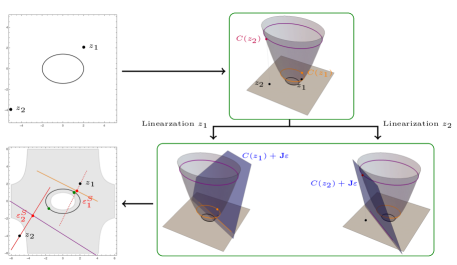
Figure 1: The model $C(x,y)=x^{2}+2y^{2}-4=0$ is the ellipse on the top left, and the data points are $z_{1}$ and $z_{2}$. The orange and purple curves in the gray surface on the top right are the points that satisfy $C(x,y)=C(\boldsymbol{z}_{1})$ and $C(x,y)=C(\boldsymbol{z}_{2})$ respectively. In the bottom right the blue planes are the tangent planes to $C(\boldsymbol{z}_{1})$ and $C(\boldsymbol{z}_{2})$ respectively. The orange and purple lines are the linearized constraints for $z_{1}$ and $z_{2}$ respectively. We keep this color convention for the linearized constraints on the bottom right, and represent their normals in red. The Sampson approximations for $z_{1}$ and $z_{2}$ are the red points $\boldsymbol{\varepsilon}_{1}^{S}$ and $\boldsymbol{\varepsilon}_{2}^{S}$ respectively. The geometric errors are depicted in green. Since $\boldsymbol{z}_{1}$ is inside the gray region, its Sampson approximation is better than the approximation for $\boldsymbol{z}_{2}$.

For the specific case of the epipolar constraint, the optimal solution to (2) can be computed [9, 15] by finding the roots to degree 6 univariate polynomial. As this procedure is relatively expensive, and difficult to integrate into non-linear refinement methods, it is common in practice to instead use some approximation of the error in (2). One example of this is the Sampson error [21, 16], defined as

$$\mathcal{E}^{2}_{S}=\frac{(({\boldsymbol{x}}_{2};1)^{\intercal}\boldsymbol{E}({\boldsymbol{x}}_{1};1))^{2}}{\|\boldsymbol{E}_{12}({\boldsymbol{x}}_{1};1)\|^{2}+\|(\boldsymbol{E}^{\intercal})_{12}({\boldsymbol{x}}_{2};1)\|^{2}}.$$ (4)

This expression is derived by linearizing the constraint in (2), i.e. by replacing $C(\hat{\boldsymbol{x}}_{1},\hat{\boldsymbol{x}}_{2},E)=0$ by the constant and linear terms of its Taylor expansion around the data point $(\boldsymbol{x}_{1},\boldsymbol{x}_{2})$. It provides a good approximation of (2) if the curvature of the constraint at the data point is small enough in relation to the size of $C(\boldsymbol{x}_{1},\boldsymbol{x}_{2},E)$, while being cheap to compute and easy to optimize in non-linear refinement. This approach was originally used by Sampson [21] to approximate distances between conics and points, but has since been applied to many other geometric models.

In this paper we revisit the Sampson approximation and provide new theoretical insights into why (and when) the approximation works well. Under relatively mild assumptions we derive explicit bounds on the tightness of the approximation. These bounds are experimentally validated on real data and showcased in multiple applications from geometric computer vision (two- and three-view estimation, vanishing point estimation and resectioning).

The paper is organized as follows: Section 1.1 discusses the related work. In Section 2 we first present the classical derivation of the Sampson error, along with some geometrical interpretations of the approximation. In Section 3 we present our bounds on the approximation. Finally, in Section 4 we provide some experimental evaluation.

1.1 Related Work

The Geometric Error.

In applied algebraic geometry, fitting noisy data points to a mathematical model defined by polynomials has recently seen a lot of interest [6], and more specifically for 3D reconstruction [17, 20]. One of the main contributions is the development and computation of the so called Euclidean distance degree, which is the number of critical points to the closest point optimization problem given generic data. It expresses the algebraic complexity of fitting data to a model; the higher the Euclidean distance degree is, the more computationally expensive this optimization is. It is used to implement efficient solvers in Homotopy Continuation [2]. Alternatively, solving the associated polynomials systems can be done via specialized symbolic solvers [13].

The Sampson Error.

The Sampson approximation was first proposed in [21] to approximate the point-conic distance. It was also later derived independently by Taubin [26]. Since then it has appeared in numerous papers for different problems. Luong and Faugeras [16] introduced it for approximating the reprojection error in epipolar geometry. The corresponding geometric error for homographies was first introduced by Sturm [24] and later revisited by Chum et al. [4] who also dervied the Sampson approximation in this setting. Leonardos et al. [14] used the Sampson error for point-line-line constraint from the trifocal tensor. Chojnacki et al. [3] considered how to integrate known measurement covariances, and recently Terekhov et al. [27] generalized the Sampson error in epipolar geometry to handle arbitrary central camera model. In [25] it was used in an optimization method for conic fitting that guarantees convergence to an ellipse. This extensive use of the Sampson approximation for geometric problems shows its versatility, which motivates a deeper theoretical study in a more general setting. This is precisely our goal in this work.

2 The Sampson Approximation

We consider geometric residuals analogous to (2) for general models, i.e. problems of the form

$$\mathcal{E}_{G}^{2}(\boldsymbol{z},\boldsymbol{\theta})=\min_{\boldsymbol{\varepsilon}}\quad \left\|\boldsymbol{\varepsilon}\right\|^{2}$$ (5)

s.t. $$C(\boldsymbol{z}+\boldsymbol{\varepsilon},\boldsymbol{\theta})=0$$ (6)

where $\boldsymbol{z}\in\mathbb{R}^{N}$ is our measurement, $\boldsymbol{\theta}$ our model parameters, and $C(\boldsymbol{z},\boldsymbol{\theta})$ our geometric constraint. In the special case of epipolar geometry, we have that $\boldsymbol{z}=[\boldsymbol{x}_{1},\boldsymbol{x}_{2}]$ consists of the two matching image points, our model is the essential matrix $\boldsymbol{E}$ and the constraint is,

$$C(\boldsymbol{z},\boldsymbol{E})=(\boldsymbol{{x}}_{2};1)^{\intercal}\boldsymbol{E}(\boldsymbol{{x}}_{1};1)=0.$$ (7)

In the rest of the paper we consider a general polynomial constraint $C(\boldsymbol{z},\boldsymbol{\theta})$ and will for notational convenience drop the dependence on the model parameters $\boldsymbol{\theta}$ in most places.

Since (5) often does not admit a simple closed form solution, the idea in [21] is to linearize the constraint, $C(\boldsymbol{z}+\boldsymbol{\varepsilon})=0$, at the original measurement $\boldsymbol{z}$, i.e.

$$\mathcal{E}_{S}^{2}(\boldsymbol{z},\boldsymbol{E})=\min_{\boldsymbol{\varepsilon}}\quad \left\|\boldsymbol{\varepsilon}\right\|^{2}$$ (8)

s.t. $$C(\boldsymbol{z})+\boldsymbol{J}\boldsymbol{\varepsilon}=0$$ (9)

where $\boldsymbol{J}=\partial C(\boldsymbol{z})/\partial\boldsymbol{z}$ is the Jacobian of the constraint, evaluated at $\boldsymbol{z}$. Introducing a Lagrangian for (8),

$$\mathcal{L}(\boldsymbol{\varepsilon},\lambda)=\frac{1}{2}\left\|\boldsymbol{\varepsilon}\right\|^{2}+\lambda\left(C(\boldsymbol{z})+\boldsymbol{J}\boldsymbol{\varepsilon}\right)$$ (10)

we get the first-order constraints as

$$\boldsymbol{\varepsilon}+\lambda\boldsymbol{J}^{\intercal}=0,\quad C(\boldsymbol{z})+\boldsymbol{J}\boldsymbol{\varepsilon}=0.$$ (11)

Inserting the first equation into the second yields,

$$C(\boldsymbol{z})-\lambda\|\boldsymbol{J}\|^{2}=0\implies\boldsymbol{\varepsilon}=-\frac{C(\boldsymbol{z})}{\|\boldsymbol{J}\|^{2}}\boldsymbol{J}^{\intercal}.$$ (12)

Thus the minimum in (8) is given by

$$\mathcal{E}_{S}^{2}=\left\|\frac{C(\boldsymbol{z})}{\|\boldsymbol{J}\|^{2}}\boldsymbol{J}^{\intercal}\right\|^{2}=\frac{C(\boldsymbol{z})^{2}}{\|\boldsymbol{J}\|^{2}}.$$ (13)

In the special case of epipolar geometry, replacing $C(\boldsymbol{z})$ with the epipolar constraint, we arrive at the classical formula for the Sampson error (4).

2.1 Multiple Constraints and Covariances

The Sampson error for a single constraint, discussed previously, can easily be generalized to the case where we measure the deviation in the Mahalanobis distance from a model defined by multiple constraints. See [8, p128] for more details. Assume that the $N$ constraints are given by

$$\boldsymbol{C}(\boldsymbol{z})=\left(C_{1}(\boldsymbol{z}),C_{2}(\boldsymbol{z}),~{}\dots,C_{N}(\boldsymbol{z})\right)^{\intercal}=\boldsymbol{0}$$ (14)

and we want to measure the deviation $\boldsymbol{\varepsilon}$ in Mahalanobis distance for a given covariance ${\boldsymbol{\Sigma}}$. This can be formulated as

$$\mathcal{E}_{G}^{2}(\boldsymbol{z},\boldsymbol{E})=\min_{\boldsymbol{\varepsilon}}\quad \left\|\boldsymbol{\varepsilon}\right\|^{2}_{\boldsymbol{\Sigma}}$$ (15)

s.t. $$\boldsymbol{C}(\boldsymbol{z}+\boldsymbol{\varepsilon})=\boldsymbol{0}$$ (16)

where $\left\|\boldsymbol{\varepsilon}\right\|^{2}_{\boldsymbol{\Sigma}}=\boldsymbol{\varepsilon}^{\intercal}{\boldsymbol{\Sigma}}^{-1}\boldsymbol{\varepsilon}$. The Lagrangian of the linearized constraint then becomes

$$\mathcal{L}(\boldsymbol{\varepsilon},\boldsymbol{\lambda})=\frac{1}{2}\left\|\boldsymbol{\varepsilon}\right\|^{2}_{\boldsymbol{\Sigma}}+\boldsymbol{\lambda}^{\intercal}\left(\boldsymbol{C}(\boldsymbol{z})+\boldsymbol{J}\boldsymbol{\varepsilon}\right)$$ (17)

where $\boldsymbol{J}\in\mathbb{R}^{N\times n}$ is the jacobian of $\boldsymbol{C}$ evaluated at $\boldsymbol{z}\in\mathbb{R}^{n}$. First order conditions again yield,

$${\boldsymbol{\Sigma}}^{-1}\boldsymbol{\varepsilon}+\boldsymbol{J}^{\intercal}\boldsymbol{\lambda}=\boldsymbol{0},\quad\boldsymbol{C}(\boldsymbol{z})+\boldsymbol{J}\boldsymbol{\varepsilon}=\boldsymbol{0}$$ (18)

We get $\boldsymbol{\varepsilon}=-{\boldsymbol{\Sigma}}\boldsymbol{J}^{\intercal}\boldsymbol{\lambda}$, allowing us to solve for $\boldsymbol{\lambda}$ as

$$\boldsymbol{C}(\boldsymbol{z})-\boldsymbol{J}{\boldsymbol{\Sigma}}\boldsymbol{J}^{\intercal}\boldsymbol{\lambda}=\boldsymbol{0}\implies\boldsymbol{\lambda}=(\boldsymbol{J}{\boldsymbol{\Sigma}}\boldsymbol{J}^{\intercal})^{-1}\boldsymbol{C}(\boldsymbol{z}).$$ (19)

This step depends on $\boldsymbol{J}{\boldsymbol{\Sigma}}\boldsymbol{J}^{\intercal}$ being invertible. In Section 2.2 we consider the general case. From this we get

$$\boldsymbol{\varepsilon}^{S}=-{\boldsymbol{\Sigma}}\boldsymbol{J}^{T}(\boldsymbol{J}{\boldsymbol{\Sigma}}\boldsymbol{J}^{\intercal})^{-1}\boldsymbol{C}(\boldsymbol{z})$$ (20)

and finally, $\|\boldsymbol{\varepsilon}^{S}\|_{\boldsymbol{\Sigma}}^{2}=\boldsymbol{\varepsilon}^{S}{\boldsymbol{\Sigma}}^{-1}\boldsymbol{\varepsilon}^{S}$ which simplifies to

$$\boldsymbol{C}(\boldsymbol{z})^{\intercal}(\boldsymbol{J}{\boldsymbol{\Sigma}}\boldsymbol{J}^{\intercal})^{-1}\boldsymbol{C}(\boldsymbol{z})=\|\boldsymbol{C}(\boldsymbol{z})\|^{2}_{\boldsymbol{J}\Sigma\boldsymbol{J}^{\intercal}}.$$ (21)

2.2 General Case

Let $(\cdot)^{\dagger}$ denote the Moore-Penrose psuedo-inverse of a matrix. Assuming that the linearized equation $\boldsymbol{C}(\boldsymbol{z})+\boldsymbol{J}\boldsymbol{\varepsilon}=\boldsymbol{0}$ has at least one solution, meaning that $\boldsymbol{C}(\boldsymbol{z})\in\text{Im}\;\boldsymbol{J}=\text{Im}\;\boldsymbol{J}{\boldsymbol{\Sigma}}^{1/2}$, then $(\boldsymbol{J}{\boldsymbol{\Sigma}}^{1/2})(\boldsymbol{J}{\boldsymbol{\Sigma}}^{1/2})^{\dagger}\boldsymbol{C}(\boldsymbol{z})=\boldsymbol{C}(\boldsymbol{z})$. In this case, all solutions to the linearized equation can be written

$$\boldsymbol{\varepsilon}(\boldsymbol{\lambda})=-{\boldsymbol{\Sigma}}^{1/2}(\boldsymbol{J}{\boldsymbol{\Sigma}}^{1/2})^{\dagger}\boldsymbol{C}(\boldsymbol{z})+N\boldsymbol{\lambda},\quad\boldsymbol{\lambda}\in\mathbb{R}^{m}$$ (22)

where the columns of $N$ is a basis for the nullspace of $\boldsymbol{J}$. In order to find $\boldsymbol{\varepsilon}^{S}$ we consider

$$\|\boldsymbol{\varepsilon}^{S}\|_{\boldsymbol{\Sigma}} =\min_{\boldsymbol{\lambda}}\|{\boldsymbol{\Sigma}}^{-1/2}\left(-{\boldsymbol{\Sigma}}^{1/2}(\boldsymbol{J}{\boldsymbol{\Sigma}}^{1/2})^{\dagger}\boldsymbol{C}(\boldsymbol{z})+N\boldsymbol{\lambda}\right)\|$$ (23)

$$=\min_{\boldsymbol{\lambda}}\|-(\boldsymbol{J}{\boldsymbol{\Sigma}}^{1/2})^{\dagger}\boldsymbol{C}(\boldsymbol{z})+{\boldsymbol{\Sigma}}^{-1/2}N\boldsymbol{\lambda}\|.$$ (24)

Here we note that $N^{\intercal}{\boldsymbol{\Sigma}}^{-1/2}(\boldsymbol{J}{\boldsymbol{\Sigma}}^{1/2})^{\dagger}=\boldsymbol{0}$, which implies that the optimal choice is $\boldsymbol{\lambda}=\vec{0}$. To be precise, we get

$$\boldsymbol{\varepsilon}^{S}=-{\boldsymbol{\Sigma}}^{1/2}(\boldsymbol{J}{\boldsymbol{\Sigma}}^{1/2})^{\dagger}\boldsymbol{C}(\boldsymbol{z}).$$ (25)

and thus

$$\|\boldsymbol{\varepsilon}^{S}\|^{2}_{\boldsymbol{\Sigma}}=\|(\boldsymbol{J}{\boldsymbol{\Sigma}}^{1/2})^{\dagger}\boldsymbol{C}(\boldsymbol{z})\|^{2}$$ (26)

Remark 2.1.

For the case of $\Sigma=I$, we note that $\|\boldsymbol{\varepsilon}^{S}\|=\|\boldsymbol{J}^{\dagger}\boldsymbol{C}(\boldsymbol{z}_{0})\|$ is the length of the Gauss-Newton step,

$$\boldsymbol{z}_{1}=\boldsymbol{z}_{0}-(\boldsymbol{J}^{\intercal}\boldsymbol{J})^{-1}\boldsymbol{J}^{\intercal}\boldsymbol{C}(\boldsymbol{z}_{0})$$ (27)

applied to solving $\boldsymbol{C}(\boldsymbol{x})=0$ starting from the point $\boldsymbol{z}$. This is visualized in Figure 1 for one constraint in two variables.

3 Bounding the Approximation Error

In this section we investigate the Sampson approximation (8) in terms of how well it approximates the geometric error (5). We do this by constructing explicit bounds. We start by studying one quadratic constraint and then we generalize our methods by considering constraints of higher degrees. Finally, we discuss the case of multiple constraints, but leave the details in the Supplementary Material.

3.1 One Quadratic Constraint

Consider the case where we have one quadratic constraint $C(\boldsymbol{z})$. The classical Sampson error (4) falls into this category as the epipolar constraint is a quadratic polynomial in terms of the image points.

We write $\boldsymbol{\varepsilon}^{G}$ for the argmin of (5) and $\boldsymbol{\varepsilon}^{S}$ for the argmin of (8). Given a fixed data point $\boldsymbol{z}\in\mathbb{R}^{n}$, we write $\vec{H}$ for the Hessian of $C$ at $\boldsymbol{z}$. Since $C$ is a quadratic polynomial,

$$C(\boldsymbol{z}+\boldsymbol{\varepsilon})=C(\boldsymbol{z})+\boldsymbol{J}\boldsymbol{\varepsilon}+\frac{1}{2}\boldsymbol{\varepsilon}^{\intercal}\vec{H}\boldsymbol{\varepsilon}.$$ (28)

We use that any vector $\boldsymbol{\varepsilon}$ satisfies the inequality

$$|\boldsymbol{\varepsilon}^{\intercal}\vec{H}\boldsymbol{\varepsilon}|\leq\rho\|\boldsymbol{\varepsilon}\|^{2}$$ (29)

where $\rho$ is the spectral radius of the Hessian of $C(\boldsymbol{z})$, that is, the maximum of the absolute values of its eigenvalues.

First we present an upper bound on the Sampson approximation $\|\boldsymbol{\varepsilon}^{S}\|$ in terms of the geometric residual $\|\boldsymbol{\varepsilon}^{G}\|$.

Proposition 3.1.

When the optimization problem (5) only has one quadratic constraint and $\boldsymbol{J}\neq 0$, then

$$\|\boldsymbol{\varepsilon}^{S}\|\leq\|\boldsymbol{\varepsilon}^{G}\|+\frac{\rho}{2\|\boldsymbol{J}\|}\|\boldsymbol{\varepsilon}^{G}\|^{2}.$$ (30)

Under the assumption that $\rho/2\|\boldsymbol{J}\|$ is reasonably small (i.e. function is approximately linear), we can interpret this proposition as saying that if $\boldsymbol{\varepsilon}^{S}$ is big, then $\boldsymbol{\varepsilon}^{G}$ is also big.

The condition $\boldsymbol{J}\neq 0$ is reasonable, as the approximation is undefined if the linearized constraint set is empty.

Proof.

Since $\boldsymbol{\varepsilon}^{G}$ satisfies the constraint (28), we have that

$$0= ~{}C(\boldsymbol{z})+\boldsymbol{J}\boldsymbol{\varepsilon}^{G}+\frac{1}{2}(\boldsymbol{\varepsilon}^{G})^{\intercal}\vec{H}\boldsymbol{\varepsilon}^{G}$$ (31)

$$= ~{}C(\boldsymbol{z})+\boldsymbol{J}\Big{(}\boldsymbol{\varepsilon}^{G}+\frac{\boldsymbol{J}^{\intercal}}{\|\boldsymbol{J}\|^{2}}\frac{1}{2}(\boldsymbol{\varepsilon}^{G})^{\intercal}\vec{H}\boldsymbol{\varepsilon}^{G}\Big{)}.$$ (32)

In other words, $\boldsymbol{\varepsilon}^{G}+\frac{\boldsymbol{J}^{\intercal}}{\|\boldsymbol{J}\|^{2}}\frac{1}{2}(\boldsymbol{\varepsilon}^{G})^{\intercal}\vec{H}\boldsymbol{\varepsilon}^{G}$ satisfies the linearized constraint. Since $\boldsymbol{\varepsilon}^{S}$ is by definition the smallest vector that satisfies the linearized constraint, we get that

$$\|\boldsymbol{\varepsilon}^{S}\|\leq\|\boldsymbol{\varepsilon}^{G}\|+\frac{1}{2\|\boldsymbol{J}\|}|(\boldsymbol{\varepsilon}^{G})^{\intercal}\vec{H}\boldsymbol{\varepsilon}^{G}|.$$ (33)

Finally, using the inequality of the spectral radius $\rho$ mentioned above, we get the upper bound. ∎

Next we give an upper bound of $\|\boldsymbol{\varepsilon}^{G}\|$ in terms of $\|\boldsymbol{\varepsilon}^{S}\|$.

Proposition 3.2.

If the minimization problem (5) only has one quadratic constraint,

$$\boldsymbol{J}\neq 0\textnormal{ and }\|\boldsymbol{J}\|^{4}\geq 2|C(\boldsymbol{z})||\boldsymbol{J}\vec{H}\boldsymbol{J}^{\intercal}|,$$ (34)

then

$$\|\boldsymbol{\varepsilon}^{G}\|\leq 2\|\boldsymbol{\varepsilon}^{S}\|.$$ (35)

The assumption should be intuitively understood as the model being close enough to linear in the direction of $\boldsymbol{J}$ locally around the input $\boldsymbol{z}$, relative to the size of $C(\boldsymbol{z})$. Note that from the Proposition, we also have

$$\|\boldsymbol{\varepsilon}^{S}-\boldsymbol{\varepsilon}^{G}\|\leq\|\boldsymbol{\varepsilon}^{S}\|+\|\boldsymbol{\varepsilon}^{G}\|\leq 3\|\boldsymbol{\varepsilon}^{S}\|.$$ (36)

Proof.

Define $\boldsymbol{\varepsilon}(\lambda):=\frac{\lambda}{\|\boldsymbol{J}\|}\boldsymbol{J}^{\intercal}$ for $\lambda\in\mathbb{R}$ and consider

$$C(\boldsymbol{z}+\boldsymbol{\varepsilon}(\lambda))=C(\boldsymbol{z})+\|\boldsymbol{J}\|\lambda+\frac{\boldsymbol{J}\vec{H}\boldsymbol{J}^{\intercal}}{2\|\boldsymbol{J}\|^{2}}\lambda^{2},$$ (37)

which is a quadratic polynomial in $\lambda$. Evaluating this polynomial at $\lambda=-2C(\boldsymbol{z})/\|\boldsymbol{J}\|$, we get

$$-C(\boldsymbol{z})+2\frac{\boldsymbol{J}\vec{H}\boldsymbol{J}^{\intercal}}{\|\boldsymbol{J}\|^{4}}C(\boldsymbol{z})^{2}.$$ (38)

The absolute value of the second term can by assumption be bounded from above by $|C(\boldsymbol{z})|$. This means that either $C(\boldsymbol{z})\geq 0$ and $C(\boldsymbol{z}+\boldsymbol{\varepsilon}(-2C(\boldsymbol{z})/\|\boldsymbol{J}\|))\leq 0$ or the other way around. By continuity of polynomials, there must exist a solution $\lambda^{*}$ to (37) in the interval $\Big{[}0,-2|C(\boldsymbol{z})|/\|\boldsymbol{J}\|\Big{]}$. Since $\boldsymbol{\varepsilon}^{G}$ is the smallest vector satisfying this, we have

$$\|\boldsymbol{\varepsilon}^{G}\|\leq\|\boldsymbol{\varepsilon}(\lambda^{*})\|=|\lambda^{*}|\leq 2|C(\boldsymbol{z})|/\|\boldsymbol{J}\|=2\|\boldsymbol{\varepsilon}^{S}\|.$$ (39)

∎

In order to get a sharper bound in the case that $\boldsymbol{J}\boldsymbol{H}\boldsymbol{J}^{\intercal}\neq 0$, we may instead solve the quadratic equation (37) directly:

$$\lambda^{*}=\frac{-\|\boldsymbol{J}\|^{3}\pm\|\boldsymbol{J}\|\sqrt{\|\boldsymbol{J}\|^{4}-2C(\boldsymbol{z})\boldsymbol{J}\vec{H}\boldsymbol{J}^{\intercal}}}{\boldsymbol{J}\boldsymbol{H}\boldsymbol{J}^{\intercal}}.$$ (40)

Let $\lambda^{*}$ be the solution with smallest absolute value, then $\|\boldsymbol{\varepsilon}^{G}\|\leq|\lambda^{*}|$ and, following from the proof of Proposition 3.2, $|\lambda^{*}|\leq 2\|\boldsymbol{\varepsilon}^{S}\|$. Note that if $\boldsymbol{J}\vec{H}\boldsymbol{J}^{\intercal}=0$, then $\lambda^{*}=-C(\boldsymbol{z})/\|\boldsymbol{J}\|$ and we directly get $\|\boldsymbol{\varepsilon}^{G}\|\leq\|\boldsymbol{\varepsilon}^{S}\|$.

To summarize we have the following inequalities

$$\frac{1}{2}\|\boldsymbol{\varepsilon}^{G}\|\leq\frac{1}{\tau}\|\boldsymbol{\varepsilon}^{G}\|\leq\|\boldsymbol{\varepsilon}^{S}\|\leq\|\boldsymbol{\varepsilon}^{G}\|+\frac{\rho}{2\|\boldsymbol{J}\|}\|\boldsymbol{\varepsilon}^{G}\|^{2},$$ (41)

where $\tau=|\lambda^{*}/C(\boldsymbol{z})|\,\|\boldsymbol{J}\|$ and $\lambda^{*}$ is given by (40).

The hypothesis in Proposition 3.2 defines a region where the geometric error is bounded linearly by the Sampson error. We highlight that this region contains the region defined by

$$\|\boldsymbol{\varepsilon}^{S}\|=\frac{|C(\boldsymbol{z})|}{\|\boldsymbol{J}\|}\leq\frac{\|\boldsymbol{J}\|}{2\rho}.$$ (42)

Example 3.3.

Consider as a constraint the conic $C(\boldsymbol{x})=x_{1}^{2}+2x_{2}^{2}-4$ in $\mathbb{R}^{2}$. For fixed $\boldsymbol{z}=(z_{1},z_{2})$, the minimization problem is

$$\min_{\boldsymbol{\varepsilon}}\quad \left\|\boldsymbol{\varepsilon}\right\|^{2}$$ (43)

s.t. $$(z_{1}+\varepsilon_{1})^{2}+2(z_{2}+\varepsilon_{2})^{2}-4=0$$ (44)

and the linearized constraint is

$$z_{1}^{2}+2z_{2}^{2}-4+\begin{bmatrix}2z_{1}&4z_{2}\end{bmatrix}\begin{bmatrix}\varepsilon_{1}\\ \varepsilon_{2}\end{bmatrix}=0.$$ (45)

From Proposition 3.2 we have that $\|\boldsymbol{\varepsilon}^{G}\|\leq 2\|\boldsymbol{\varepsilon}^{S}\|$ if $\boldsymbol{z}$ is in the colored region of Figure 2 (both the orange and purple region). Finally, the relaxed condition from (42) gives a smaller region, potentially easier to work with, where the previous bounds also hold, this is the purple region in Figure 2

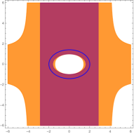
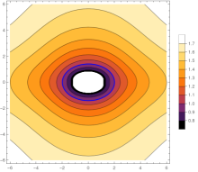
Figure 2: Regions obtained for Example 3.3. On the left, the constraint $x_{1}^{2}+2x_{2}^{2}-4=0$ is depicted in blue, the purple region is obtained from Equation 42 and it is contained in the orange region coming from Equation 35. On the right, the level sets for the ratio $\|\boldsymbol{\varepsilon}^{G}\|/\|\boldsymbol{\varepsilon}^{S}\|$, and the constraint depicted in blue. Observe that, although the ratio changes, it is bounded by 2 for every point in the colored regions.

3.2 One Polynomial Constraint

To understand the Sampson error for a model defined by a single polynomial constraint of any degree $C:\mathbb{R}^{n}\to\mathbb{R}$, we extend the method presented previously and consider Taylor approximations of degree $d$:

$$C(\boldsymbol{z}+\boldsymbol{\varepsilon})=C(\boldsymbol{z})+\sum_{i=1}^{d}\frac{1}{i!}\boldsymbol{\varepsilon}\times\mathcal{T}_{i},$$ (46)

where $\mathcal{T}_{i}$ is a symmetric $n\times\cdots\times n$ tensor of order $i$. For example, $\mathcal{T}_{1}=\boldsymbol{J}$ is the Jacobian, $\mathcal{T}_{2}=\vec{H}$ the Hessian, and

$$\boldsymbol{\varepsilon}\times\mathcal{T}_{i}=\sum_{j_{1},\ldots,j_{i}\in[n]}(\mathcal{T}_{i})_{j_{1},\ldots,j_{i}}\varepsilon_{j_{1}}\cdots\varepsilon_{j_{i}}.$$ (47)

Proposition 3.4.

When the optimization problem (5) only has one polynomial constraint of degree $d$,

$$\boldsymbol{J}\neq 0\textnormal{ and }|C(\boldsymbol{z})|\geq\Big{|}\sum_{i=2}^{d}(-1)^{i}\frac{2^{i}C(\boldsymbol{z})^{i}}{i!\|\boldsymbol{J}\|^{i}}\boldsymbol{J}\times\mathcal{T}_{i}\Big{|},$$ (48)

then $\|\boldsymbol{\varepsilon}^{G}\|\leq 2\|\boldsymbol{\varepsilon}^{S}\|.$

Proof.

The proof is exactly the same as for Proposition 3.2; one checks that $C(\boldsymbol{z})\leq 0$ and $C(\boldsymbol{z}+\boldsymbol{\varepsilon}(\lambda))\geq 0$ (or the other way around) for $\lambda=-2C(\boldsymbol{z})/\|\boldsymbol{J}\|$. ∎

3.3 Multiple Polynomial Constraints

For mathematical models defined by multiple constraints, the Sampson error and its relation to the geometric error are more involved. Here, we give an overview of our approach to computing Sampson errors in practice and studying its relation to the geometric error for polynomial constraints, but leave mathematical statements and proofs in the Supplementary Material.

Assume that $\boldsymbol{C}(\boldsymbol{z})=(C_{1}(\boldsymbol{z}),\ldots,C_{N}(\boldsymbol{z}))$ are $N$ polynomial constraints. The model $\boldsymbol{C}(\boldsymbol{z})=\vec{0}$, for $\boldsymbol{z}\in\mathbb{R}^{n}$, is an algebraic variety $X$ (a zero set of a system of polynomials) of some dimension $d\leq n$, which depends on the constraints. For generic constraints of fixed degrees $d=n-N$, i.e. each constraint lowers the dimension of the model by one, however, for specific systems of polynomials this equality does not necessarily hold. In both cases, the intuitive behaviour is that the more constraints we have, the smaller $d$ is and our data is harder to fit to the model. The same phenomenon occurs with the linearized constraints for the Sampson error, the more constraints we have, the smaller is the affine linear space defined by $\boldsymbol{C}(\boldsymbol{z})+\boldsymbol{J}\boldsymbol{\varepsilon}=0$. Therefore, if $N$ is much greater than $n-d$, the Sampson approximation is likely to be poor. To remedy this, we propose to use the fact that locally around a generic point of $X$, the model is described by precisely $n-d$ polynomials whose Jacobian has full rank. This is a result coming from algebraic geometry. Our proposal is to perform Sampson approximation by choosing a subset of $n-d$ constraints whose Jacobian is full-rank and linearizing those constraints. In Section 4.2 we try this approach for the Three-View Sampson error and the results suggest that it is also beneficial to choose these constraints with smallest degree possible.

In the Supplementary Material, we generalize Proposition 3.1 and find an upper bound for $\|\boldsymbol{\varepsilon}^{S}\|$ in terms of $\|\boldsymbol{\varepsilon}^{G}\|$ for multiple constraints of any degrees. We also generalize Proposition 3.2 for quadratic constraints and data points $\boldsymbol{z}$ such that the Jacobian $\boldsymbol{J}$ at $\boldsymbol{z}$ has linearly independent rows. In this case, under appropriate conditions, we find a $\boldsymbol{\lambda}^{*}$ such that $C_{i}(\boldsymbol{z}+\|\boldsymbol{J}\|\boldsymbol{J}^{\dagger}\boldsymbol{\lambda}^{*})=0$ for $i=1,\ldots,n$. We get

$$\|\boldsymbol{\varepsilon}^{G}\|\leq\|\|\boldsymbol{J}\|\boldsymbol{J}^{\dagger}\boldsymbol{\lambda}^{*}\|\leq\|\boldsymbol{J}\|\|\boldsymbol{J}^{\dagger}\|\|\boldsymbol{\lambda}^{*}\|,$$ (49)

and by construction we get an upper bound for this $\|\boldsymbol{\lambda}^{*}\|$ expressed in terms of $\boldsymbol{C}$, its Jacobian and its Hessian.

4 Experimental Evaluation

In the following sections we evaluate the Sampson approximation for different geometric estimation problems. First, in Section 4.1 we evaluate the classical Sampson error for two-view geometry. Next, in Section 4.2 we consider the analogous error in the three-view setting. Section 4.3 considers line segment to vanishing point errors. Finally, Section 4.4 show an application from absolute pose estimation with uncertainties applied in both 2D and 3D.

4.1 Application: Two-view Relative Pose

We first consider the classical setting where the Sampson approximation is applied, two-view relative pose estimation. For the experiment we use $\sim$5k image pairs from the British Museum scene in the Image Matching Challenge (IMC) 2021 [11]. For each image pair we estimate an initial essential matrix using DLT [8] applied to the ground truth inliers. For each correspondence we compute the true reprojection error $\mathcal{E}_{G}$ using optimal triangulation [15].

Results and Discussion. Figure 3 shows the distribution of the difference between the Sampson approximation and the true error, and in Table 1 shows the Area-Under-Curve up to 1 pixel. For comparison we also include the symmetric epipolar error (distances to the epipolar lines computed in both images) which is another popular choice in practice. The Sampson error provides a very accurate approximation of the true reprojection error. As discussed in Section 3 the quality of the approximation depend on the how close the initial point is to the constraint set (small $C(\boldsymbol{z})$) and the curvature (small hessian). In Figure 4 we plot the approximation error $|\mathcal{E}_{S}-\mathcal{E}_{G}|$ against $\rho|C(\boldsymbol{z})|/\|J\|^{2}$, where $\rho$ is the spectral norm of the hessian. Consistent with the theory, the figure shows a clear trend where correspondences with smaller $\rho|C(\boldsymbol{z})|/\|J\|^{2}$ have smaller errors.

Finally we also evaluate the error in the context of pose refinement. Table 2 shows the resulting pose errors (max of rotation and translation error) after non-linear refinement of the initial essential matrix using different error functions. Algebraic is the squared epipolar constraints. Cosine is the squared cosine of the angles between the normals of the epipolar planes and the point correspondences. The Sampson error provides the most accurate camera poses.

Figure 3: Approximation gap for two-view relative pose. Comparison with optimal triangulation [15]. The unit is in pixels. Here $\mathcal{E}$ refers to either the Sampson or the symmetric epipolar error.

	$|\mathcal{E}-\mathcal{E}_{G}|$,   AUC @ $\tau$ px ($\uparrow$)
Error	$\tau=0.1$	$\tau=0.5$	$\tau=1$
Sampson	0.991	0.998	0.999
Symmetric Epipolar	0.620	0.839	0.902

Table 1: The table shows the Area-Under-Curve of the approximation error $|\mathcal{E}-\mathcal{E}_{G}|$ up to different thresholds.

Figure 4: Approximation error against $\rho|C(\boldsymbol{z})|/\|J\|^{2}$ for two-view relative pose. Figure shows a heatmap built from the inlier correspondences of $\sim$5k image pairs from the British Museum scene. Points that are either close to satisfying the epipolar constraint ($C(\boldsymbol{z})\approx 0$) or have low curvature ($\rho$) have smaller errors.

	Pose error AUC ($\uparrow$)
	@5∘	@10∘	@20∘
Initial estimate (DLT)	0.184	0.292	0.414
$\Lsh$ Algebraic	0.375	0.459	0.533
$\Lsh$ Cosine	0.455	0.541	0.608
$\Lsh$ Sym. Epipolar	0.465	0.552	0.621
$\Lsh$ Sampson	0.468	0.557	0.625

Table 2: Comparison of losses for two-view relative pose refinement on IMC British Museum. The initial pose is found by linear estimate (DLT) applied to the inlier correspondences (w.r.t. ground truth pose), followed by non-linear refinement.

4.2 Application: Three-view Sampson Error

In this section we evaluate different error formulations for 3-view point matches. The naive baseline is to simply average the two-view Sampson errors (4), $\quad\mathcal{E}_{pair}=~{}~{}$

$$\mathcal{E}_{S}(\boldsymbol{x},\boldsymbol{x}^{\prime},E_{12})+\mathcal{E}_{S}(\boldsymbol{x},\boldsymbol{x}^{\prime\prime},E_{13})+\mathcal{E}_{S}(\boldsymbol{x}^{\prime},\boldsymbol{x}^{\prime\prime},E_{23})$$ (50)

where $(\boldsymbol{x},\boldsymbol{x}^{\prime},\boldsymbol{x}^{\prime\prime})$ is the correspondence and $E_{ij}$ are the essential matrices. For a given a trifocal tensor $\mathcal{T}\in\mathbb{R}^{3\times 3\times 3}$ with slices $\mathtt{T}_{1},\mathtt{T}_{2},\mathtt{T}_{3}\in\mathbb{R}^{3\times 3}$, a consistent three-view point correspondence $\boldsymbol{x},\boldsymbol{x}^{\prime},\boldsymbol{x}^{\prime\prime}$ satisfies

$$\boldsymbol{C}_{9}(\boldsymbol{x},\boldsymbol{x}^{\prime},\boldsymbol{x}^{\prime\prime})=[\hat{\boldsymbol{x}}^{\prime}]_{\times}\left(\sum_{k}\hat{\boldsymbol{x}}_{k}\mathtt{T}_{k}\right)[\hat{\boldsymbol{x}}^{\prime\prime}]_{\times}=\boldsymbol{0}$$ (51)

where $\hat{\boldsymbol{x}}=[\boldsymbol{x};1]$ is the homogenization of the 2D point $\boldsymbol{x}\in\mathbb{R}^{2}$. While we have nine equations, only four are linearly independent. These can be obtained by multiplying with two $3\times 2$ matrices,

$$\boldsymbol{C}_{4}(\boldsymbol{x},\boldsymbol{x}^{\prime},\boldsymbol{x}^{\prime\prime})=S_{1}^{\intercal}[\hat{\boldsymbol{x}}^{\prime}]_{\times}\left(\sum_{k}\hat{\boldsymbol{x}}_{k}\mathtt{T}_{k}\right)[\hat{\boldsymbol{x}}^{\prime\prime}]_{\times}S_{2}$$ (52)

where $S_{1},S_{2}\in\mathbb{R}^{3\times 2}$ contains a basis for the complement of the left and right nullspace of $\boldsymbol{C}_{9}$ respectively. Another alternative is to only consider the three pairwise constraints,

$$\small\boldsymbol{C}_{3}(\boldsymbol{x},\boldsymbol{x}^{\prime},\boldsymbol{x}^{\prime\prime})=\left[\boldsymbol{x}^{\prime\intercal}E_{12}\boldsymbol{x},~{}\boldsymbol{x}^{\prime\prime\intercal}E_{13}\boldsymbol{x},~{}\boldsymbol{x}^{\prime\prime\intercal}E_{23}\boldsymbol{x}^{\prime}\right]$$ (53)

Note that applying the Sampson approximation to $\boldsymbol{C}_{3}$ yields a different error compared to $\mathcal{E}_{pair}$ (50), as the constraints are considered jointly.

In this section we evaluate the following errors

• $\mathcal{E}_{pair}$ - averaging the pairwise Sampson errors (50)

• $\mathcal{E}_{9}$ - applying Sampson approximation to $\boldsymbol{C}_{9}$ (51)

• $\mathcal{E}_{4}$ - applying Sampson approximation to $\boldsymbol{C}_{4}$ (52)

• $\mathcal{E}_{3}$ - applying Sampson approximation to $\boldsymbol{C}_{3}$ (53)

We also include two combinations of the above. First taking 3 out of the 4 constraints from $\boldsymbol{C}_{4}$, denoted $\boldsymbol{C}_{4:3}$, and one where we combine $\boldsymbol{C}_{3}$ and $\boldsymbol{C}_{4}$ by taking two quadratic and one cubic constraint, denoted $\boldsymbol{C}_{4:1,3:2}$. We also consider a set of psuedo-Sampson approximations which take the form $\|\boldsymbol{C}\|^{2}/\|\boldsymbol{J}\|^{2}$, and thus avoid computing matrix inverses as in Section 2.2. This can be seen as a naive extension of the 1-dimensional Sampson approximation (8) to the multi-dimensional case. We denote these as $\hat{\mathcal{E}_{9}},\hat{\mathcal{E}_{4}},\hat{\mathcal{E}_{3}}$.

Experiment setup. To compare the approximations we generate synthetic camera triplets (70^∘ field-of-view, 1000x1000 pixel images) observing a 3D point. To the three projections we add normally distributed noise with standard deviation $\sigma\in\{1,5,10\}$ px. We obtain the reference ground-truth reprojection error by directly optimizing over the 3D point. For each of the evaluated approximated error functions we compute the difference to the ground-truth.

Results and Discussion. Table 3 shows the errors for 100k synthetic instances. We compute the Area-Under-Curve up to 1 pixel deviation from the reference error. The Sampson approximation of the epipolar constraints $\boldsymbol{C}_{3}$ (53) yields the best approximation. In particular, we can see that the naive approximation $\mathcal{E}_{pair}$ that averages the pairwise Sampson errors, is significantly worse. Interestingly, we can also see that $\boldsymbol{C}_{4}$ performs much worse compared to both $\boldsymbol{C}_{3}$ and the mixed variants $\boldsymbol{C}_{4:3}$ and $\boldsymbol{C}_{4:1,3:2}$. This is consistent with the discussion in Sec. 3.3.

	$|\mathcal{E}-\mathcal{E}_{gt}|$, AUC @ 1px $(\uparrow)$
	$\sigma=1$px	$\sigma=5$px	$\sigma=10$px
$\mathcal{E}_{3}=\|J_{3}^{\dagger}\boldsymbol{C}_{3}\|$	0.998	0.961	0.882
$\mathcal{E}_{4:1,3:2}=\small\|J_{4:1,3:2}^{\dagger}\boldsymbol{C}_{4:1,3:2}\|$	0.995	0.937	0.830
$\mathcal{E}_{4:3}=\|J_{4:3}^{\dagger}\boldsymbol{C}_{4:3}\|$	0.994	0.912	0.768
$\mathcal{E}_{4}=\|J_{4}^{\dagger}\boldsymbol{C}_{4}\|$	0.765	0.481	0.353
$\mathcal{E}_{pair}=...$ (50)	0.764	0.312	0.172
$\hat{\mathcal{E}_{3}}=\|\boldsymbol{C}_{3}\|/\|J_{3}\|$	0.361	0.016	0.003
$\hat{\mathcal{E}_{4}}=\|\boldsymbol{C}_{4}\|/\|J_{4}\|$	0.356	0.009	0.001
$\hat{\mathcal{E}_{9}}=\|\boldsymbol{C}_{9}\|/\|J_{9}\|$	0.356	0.009	0.001
$\mathcal{E}_{9}=\|J_{9}^{\dagger}\boldsymbol{C}_{9}\|$	0.348	0.075	0.034

Table 3: Comparison of three-view reprojection error approximations. Each error metric is compared to the ground truth error (found by non-linear refinement of the 3D point). To each keypoint we add noise with standard deviation $\sigma$ pixels.

	$\tau=5$ px				$\tau=10$ px				$\tau=20$ px
	AUC $(\uparrow)$	$\varepsilon_{R}$ $(\downarrow)$	$\varepsilon_{t}$ $(\downarrow)$		AUC $(\uparrow)$	$\varepsilon_{R}$ $(\downarrow)$	$\varepsilon_{t}$ $(\downarrow)$		AUC $(\uparrow)$	$\varepsilon_{R}$ $(\downarrow)$	$\varepsilon_{t}$ $(\downarrow)$
Reprojection error (60)	0.358	1.03	3.20		0.350	1.06	3.24		0.311	1.21	3.63
Reprojection error + Cov. (61)	0.367	1.01	3.10		0.379	0.99	2.99		0.378	0.99	3.00
$\Lsh$ Sampson approximation	0.367	1.01	3.10		0.379	0.98	2.99		0.375	1.00	3.02

Table 4: Pose refinement on 7Scenes. Table shows the Area-Under-Curve (AUC) @ 5cm position errors and the median errors in rotation $\varepsilon_{R}$ (deg.) and translation $\varepsilon_{t}$ (cm). Results are reported for different inlier thresholds $\tau$. For large thresholds, more uncertain points are included and the improvement from the covariance weighting is more significant. However, larger errors also make the linearization point (the original correspondence) worse, degrading the Sampson approximation. For the two lower thresholds, the Sampson approximation of 2D-3D covariance weighted reprojection error gives almost identical results as performing the full (expensive) optimization.

4.3 Application: Vanishing Point Estimation

We now show another example with a 1-dimensional quadratic constraint. Consider a line-segment $(\boldsymbol{x}_{1},\boldsymbol{x}_{2})\in\mathbb{R}^{2}\times\mathbb{R}^{2}$ and a vanishing point $\boldsymbol{v}\in\mathbb{S}^{2}$. Assuming we want to refine $\boldsymbol{v}$, it is reasonable to consider what is the smallest pertubation of the line endpoints such that the line passes through the vanishing point, i.e. satisfy the constraint

$$C(\boldsymbol{x}_{1},\boldsymbol{x}_{2})=\boldsymbol{v}^{\intercal}(\begin{pmatrix}\boldsymbol{x}_{1}\\ 1\end{pmatrix}\times\begin{pmatrix}\boldsymbol{x}_{2}\\ 1\end{pmatrix})$$ (54)

Differentiating with respect to the image points we get,

$$\small J=\begin{bmatrix}\left(\begin{pmatrix}\boldsymbol{x}_{2}\\ 1\end{pmatrix}\times\boldsymbol{v}\right)S,&\left(\boldsymbol{v}\times\begin{pmatrix}\boldsymbol{x}_{1}\\ 1\end{pmatrix}\right)S\end{bmatrix}$$ (55)

where $S=\begin{bmatrix}I_{2}&\boldsymbol{0}\end{bmatrix}^{\intercal}$, and we can directly setup a Sampson approximation of the line-segment to vanishing point distance as $|C(\boldsymbol{x}_{1},\boldsymbol{x}_{2})|/\|\boldsymbol{J}\|$. For this problem the ground-truth error $\mathcal{E}_{G}$ can be computed in closed form using SVD.

In Section 3.1 we derived bounds that relate the true geometric error $\boldsymbol{\varepsilon}^{G}$ and the Sampson approximation $\boldsymbol{\varepsilon}^{S}$,

$$B_{l}:=\frac{1}{\tau}\leq\frac{\|\boldsymbol{\varepsilon}^{S}\|}{\|\boldsymbol{\varepsilon}^{G}\|}\leq 1+\frac{\rho}{2\|\boldsymbol{J}\|}\|\boldsymbol{\varepsilon}^{G}\|=:B_{u}$$ (56)

Next we evaluate how tight these bounds are on real data.

Experiment Setup. For the experiment we consider circa 350k pairs of line segments and vanishing points collected from the YUB+ [5] and NYU VP [18, 12]. The line segments are detected using DeepLSD [19] and using Progressive-X [1] we estimate a set of vanishing points.

Results and Discussion. Figure 6 shows $B_{u},B_{l}$ for each of line-vanishing point pairs and in Figure 6 we show the distribution of the difference between the bounds. As can be seen in the figures the approximation works extremely well for this setting. We also experimented with refining the vanishing points using the Sampson error but found that the results are very similar to minimizing the mid-point error (as was done in [19]). The full results and details can be found in the Supplementary Material.

Figure 5: Evaluation of the bounds for VP-line error. The lower bound $B_{l}$ and upper bound $B_{u}$ for the $\approx$350k VP-line pairs in the combined dataset. For illustration the pairs are sorted w.r.t. the tightness of the bound.

Figure 6: Evaluation of the bounds for VP-line error. Distribution of the $\text{log}_{10}$ differences between the upper and lower bounds.

4.4 Application: 2D/3D Reprojection Error

Minimizing the square reprojection error, i.e. deviation between the observed 2D point and the projection of the 3D point, assumes a Gaussian noise model on the 2D observations. However, in many scenarios, we also have noise in the 3D points. In this section we consider the case where we have a known covariance for both the 2D and 3D-points.

Given a point correspondence $(\boldsymbol{x},\boldsymbol{X})\in\mathbb{R}^{2}\times\mathbb{R}^{3}$, together with covariances ${\boldsymbol{\Sigma}}_{2D}\in\mathbb{R}^{2\times 2}$ and ${\boldsymbol{\Sigma}}_{3D}\in\mathbb{R}^{3\times 3}$, the maximum likelihood estimate is then given by

$$\min_{\boldsymbol{\varepsilon}_{2},\boldsymbol{\varepsilon}_{3}}\quad \left\|\boldsymbol{\varepsilon}_{2}\right\|_{{\boldsymbol{\Sigma}}_{2D}}^{2}+\left\|\boldsymbol{\varepsilon}_{3}\right\|_{{\boldsymbol{\Sigma}}_{3D}}^{2}$$ (57)

s.t. $$\boldsymbol{C}(\boldsymbol{x}+\boldsymbol{\varepsilon}_{2},\boldsymbol{X}+\boldsymbol{\varepsilon}_{3})=0$$ (58)

where $\boldsymbol{C}(\boldsymbol{x},\boldsymbol{X})$ encodes the reprojection equations, i.e.

$$\boldsymbol{C}(\boldsymbol{x},\boldsymbol{X})=[I_{2\times 2},~{}-\boldsymbol{x}]\left(R\boldsymbol{X}+\boldsymbol{t}\right)=0.$$ (59)

Experiment Setup. For the experiment we consider the visual localization benchmark setup on 7Scenes [23] dataset. Using HLoc [22] we establish 2D-3D matches and estimate an initial camera pose for each query image. For the experiment we then refine this camera pose, including the uncertainty in both the 2D and 3D points. The 2D covariances are assumed to be unit gaussians and to obtain the 3D covariances we propagate the 2D covariances from the mapping images used to triangulate the 3D point.

Results and Discussion. Table 4 shows the average pose error across all scenes (per-scene results are available in the Supplementary Material). We compare only minimizing the reprojection error (only 2D noise)

$$\min_{R,\boldsymbol{t}}\sum_{k}\|\boldsymbol{x}_{k}-\pi(R\boldsymbol{X}_{k}+\boldsymbol{t})\|^{2}_{{\boldsymbol{\Sigma}}_{2}}$$ (60)

with optimizing over the 3D points as well (2D/3D noise),

$$\min_{R,\boldsymbol{t},\{\hat{\boldsymbol{X}}_{k}\}}\sum_{k}\|\boldsymbol{x}_{k}-\pi(R\hat{\boldsymbol{X}}_{k}+\boldsymbol{t})\|^{2}_{{\boldsymbol{\Sigma}}_{2}}+\|\hat{\boldsymbol{X}}_{k}-\boldsymbol{X}_{k}\|^{2}_{{\boldsymbol{\Sigma}}_{3}}$$ (61)

and applying the Sampson approximation to (59). As shown in Table 4, including the uncertainty of the 3D point can greatly improve the pose accuracy. Further, the Sampson approximation works well in this setting and it is only when we include matches with very large errors (20 pixels) that performance degrades.

Note that the optimization problem in (61) requires parameterizing each individual 3D point, potentially leading to hundreds or thousands of extra parameters compared to (60) that only optimize over the 6-DoF in the camera pose. Since the Sampson approximation eliminates the extra unknowns, it also allows us to only optimize over the camera pose while modelling the 3D uncertainty. Figure 7 shows the average runtime in milliseconds for the query images. Minimizing the Sampson approximation is significantly faster compared to (61).

Figure 7: Runtime comparison on 7Scenes. The average runtime in milliseconds for the pose refinement experiment on 7Scenes.

5 Conclusions

The Sampson approximation, originally applied to compute conic-point distances, has shown itself to surprisingly versatile in the context of robust model fitting. While it has been known that it works extremely well in practice, we provide the first theoretical bounds on the approximation error. In multiple experiments on real data in different application contexts we have validated our theory and highlighted the usefulness of the approximation.

Appendix A Overview

In this Supplementary Material, we prove more bounds related to geometric errors

$$\mathcal{E}_{G}^{2}(\boldsymbol{z},\boldsymbol{\theta})=\min_{\boldsymbol{\varepsilon}}\quad \left\|\boldsymbol{\varepsilon}\right\|^{2}$$ (62)

s.t. $$\boldsymbol{C}(\boldsymbol{z}+\boldsymbol{\varepsilon},\boldsymbol{\theta})=0.$$ (63)

In Appendix B, we generalize Proposition 3.1 to the most general setting with $d$ constraints of any degree. In Appendix C, we give a result in the spirit of Proposition 3.2 for $N$ quadric constraints. We restrict to quadric polynomials in the case of multiple constraints, and note that this applies to the epipolar constraints.

In Appendix D we provide details regarding the optimization of Sampson approximations, and in Appendix E we show additional results from the experiments in the main paper.

Appendix B General Case Lower Bound for $\|\boldsymbol{\varepsilon}^{G}\|$

In our pursuit to understand constraints of any degrees, we make use of $d$-norms:

$$\|\boldsymbol{x}\|_{d}:=\sqrt[d]{x_{1}^{d}+\cdots+x_{n}^{d}}.$$ (64)

$\|\boldsymbol{x}\|$ refers to the $2$-norm. We make use of the following estimation of polynomials of general degrees:

Lemma B.1.

Let $q:\mathbb{R}^{n}\to\mathbb{R}$ be a homogeneous polynomial in $n$ variables of degree $d$. Then

$$|q(\boldsymbol{x})|\leq\mu_{q}\|\boldsymbol{x}\|_{d}^{d},$$ (65)

where $\mu_{q}$ is the sum of absolute values of coefficients of $q$.

This lemma can be extended to non-homogeneous polynomials in a straightforward way, by replacing $\boldsymbol{x}$ by $(\boldsymbol{x};1)$ in (65).

Proof.

Our first observation is that

$$|q(\boldsymbol{x})|\leq\big{(}\max_{\|\boldsymbol{y}\|_{d}=1}|q(\boldsymbol{y})|\big{)}\|\boldsymbol{x}\|_{d}^{d}.$$ (66)

Now $|q(\boldsymbol{y})|$ can for $\|\boldsymbol{y}\|_{d}=1$ be bounded from above by the sum of the absolute values of the coefficients of $q$. This is because for $x$ with $\|x\|_{d}=1$, each coordinate $x_{i}$ has norm $\leq 1$ and therefore the norms of monomials are bounded by $1$. ∎

We extend the notation from the main body of the paper. A set of polynomial constraints

$$\boldsymbol{C}(\boldsymbol{z})=\left(C_{1}(\boldsymbol{z}),C_{2}(\boldsymbol{z}),~{}\dots,C_{N}(\boldsymbol{z})\right)^{\intercal}=\boldsymbol{0},$$ (67)

for $\boldsymbol{z}\in\mathbb{R}^{n}$, can be expressed via a Taylor expansion:

$$C_{i}(\boldsymbol{z}+\boldsymbol{\varepsilon})=\boldsymbol{C}(\boldsymbol{z})+\sum_{j=1}^{d}\frac{1}{j!}\boldsymbol{\varepsilon}\times\mathcal{T}_{j}^{(i)},$$ (68)

for each $i$, where $\mathcal{T}_{j}^{(i)}$ is a symmetric $n\times\cdots\times n$ tensor of order $j$, and

$$\boldsymbol{\varepsilon}\times\mathcal{T}_{j}^{(i)}=\sum_{l_{1},\ldots,l_{j}\in[n]}(\mathcal{T}_{j}^{(i)})_{l_{1},\ldots,l_{j}}\varepsilon_{l_{1}}\cdots\varepsilon_{l_{j}}.$$ (69)

For example, $\mathcal{T}_{1}^{(i)}$ is the Jacobian of $C_{i}$ and $\mathcal{T}_{2}^{(i)}$ is the Hessian of $C_{i}$.

As in (69), each tensor $\mathcal{T}_{j}^{(i)}$ defines a polynomial, and by Lemma B.1,

$$|\boldsymbol{\varepsilon}\times\mathcal{T}_{j}^{(i)}|\leq\mu_{j}^{(i)}\|\boldsymbol{\varepsilon}\|_{j}^{j},$$ (70)

where $\mu_{j}^{(i)}$ is the sum of absolute values of coefficients of this polynomial. Let $\boldsymbol{\varepsilon}\times\mathcal{T}_{j}$ denote the vector of $N$ coordinates $(\boldsymbol{\varepsilon}\times\mathcal{T}_{j}^{(i)})_{i=1}^{N}$. Write $\mu_{j}$ for the sum of all $\mu_{j}^{(i)}$ for $i=1,\ldots,N$, and note that

$$|\boldsymbol{\varepsilon}\times\mathcal{T}_{j}|\leq\mu_{j}\|\boldsymbol{\varepsilon}\|_{j}^{j}.$$ (71)

Recall from Section 2.2 that putting ${\boldsymbol{\Sigma}}=I$ gives us

$$\boldsymbol{\varepsilon}^{S}=-\boldsymbol{J}^{\dagger}\boldsymbol{C}(\boldsymbol{z}).$$ (72)

Proposition B.2.

When the optimization problem (62) has $N$ homogeneous constraints of at most degree $d$ and $\boldsymbol{C}(\boldsymbol{z})\in\text{Im}\;\boldsymbol{J}$, then

$$\|\boldsymbol{\varepsilon}^{S}\|\leq\|\boldsymbol{\varepsilon}^{G}\|+\|\boldsymbol{J}^{\dagger}\|\sum_{j=2}^{d}\frac{\mu_{j}}{j!}\|\boldsymbol{\varepsilon}^{G}\|_{j}^{j}.$$ (73)

Proof.

For $\boldsymbol{\varepsilon}^{G}$, we have

$$0 =\boldsymbol{C}(z)+\boldsymbol{J}\boldsymbol{\varepsilon}^{G}+\sum_{j=2}^{d}\frac{1e}{j!}\boldsymbol{\varepsilon}^{G}\times\mathcal{T}_{j}$$ (74)

$$=\boldsymbol{C}(z)+\boldsymbol{J}\left(\boldsymbol{\varepsilon}^{G}+\boldsymbol{J}^{\dagger}\sum_{j=2}^{d}\frac{1}{j!}\boldsymbol{\varepsilon}^{G}\times\mathcal{T}_{j}\right),$$ (75)

meaning that the norm of $\boldsymbol{\varepsilon}^{S}$ must be bounded from above by the norm of

$$\boldsymbol{\varepsilon}^{G}+\boldsymbol{J}^{\dagger}\sum_{j=2}^{d}\frac{1}{j!}\boldsymbol{\varepsilon}^{G}\times\mathcal{T}_{j}.$$ (76)

However, by (71) the statement now follows. ∎

Appendix C Multiple Quadric Constraints

In this section we prove an upper bound for the geometric error in the case of multiple constraints, and take a closer look at this bound in an example with two quadric constraints. Our main tool is the following celebrated result, as stated in [10, Ch. 2, Cor. 2.15].

Theorem C.1 (Brouwer’s Fixed Point Theorem).

Every continuous function $f$ from a non-empty convex compact subset $K$ of a Euclidean space to $K$ itself has a fixed point.

Recall that a fixed point of a function is a point $x^{*}$ in the set $K$ such that $f(x^{*})=x^{*}.$ The main theorem of this section deals with varieties $X$ that are a complete intersection, defined by $N$ quadrics $\boldsymbol{C}(\boldsymbol{z})=(C_{1}(\boldsymbol{z}),\ldots,C_{N}(\boldsymbol{z}))^{\intercal}$. By complete intersection, we mean that the dimension of $X$ is $n-N$. We discuss the general case afterwards.

Let $\boldsymbol{J}^{\dagger}$ denote pseudo-inverse of the Jacobian $\boldsymbol{J}$ and let $\|\cdot\|$ denote the matrix operator norm. Define

$$\sigma_{i} :=\textnormal{ spectral radius of }\frac{\|\boldsymbol{J}\|}{2}(\boldsymbol{J}^{\dagger})^{\intercal}\boldsymbol{H}_{i}\boldsymbol{J}^{\dagger}$$ (77)

$$\text{cond}(\boldsymbol{J}) :=\|\boldsymbol{J}\|\|\boldsymbol{J}^{\dagger}\|.$$ (78)

Note neither $\sigma_{i}$ nor $\text{cond}(\boldsymbol{J})$ are independent of the individual scalings of $C_{i}$ for each $i=1,\ldots,N$. They are however independent of simultaneous scaling of all constraints.

Since we will deal with multiple constraints of degree two, we first recall a classical fact about the solutions of degree 2 equations in one variable. This will be used in the proof of the main theorem.

Remark C.2.

Consider the equation

$$\alpha x^{2}+\beta x+\gamma=0.$$ (79)

As long as $\alpha\neq 0$, the solutions to the equation are

$$x=\frac{-\beta\pm\sqrt{\beta^{2}-4\alpha\gamma}}{2\alpha}.$$ (80)

We can consider these solutions as a function of $\alpha,\beta$ and $\gamma$ that outputs a real solution to (79) for inputs in the semi-algebraic set $\beta^{2}-4\alpha\gamma\geq 0,\alpha\neq 0$. Moreover, this function is continuous because the square root is continuous too. The expression $\beta^{2}-4\alpha\gamma$ is called the discriminant of (79).

Theorem C.3.

Consider a complete intersection defined by the quadratic equations

$$\boldsymbol{C}(\boldsymbol{z})=\left(C_{1}(\boldsymbol{z}),C_{2}(\boldsymbol{z}),~{}\dots,C_{N}(\boldsymbol{z})\right)^{\intercal}=\boldsymbol{0}.$$ (81)

Assume that $\boldsymbol{J}$ is full-rank at $\boldsymbol{z}$. If a number $\kappa\geq 0$ satisfies

$$\kappa \geq\sum_{j=1}^{N}\left(\frac{|C_{j}(\boldsymbol{z})|}{\|\boldsymbol{J}\|}+\sigma_{j}\kappa\right)^{2},$$ (82)

then

$$\|\boldsymbol{\varepsilon}^{G}\|\leq\text{cond}(\boldsymbol{J})\kappa.$$ (83)

It is easy to check if there is a $\kappa$ such that the conditions (82) holds. Indeed, one solves the quadratic equation

$$\kappa =\sum_{j=1}^{N}\left(\frac{|C_{j}(\boldsymbol{z})|}{\|\boldsymbol{J}\|}+\sigma_{j}\kappa\right)^{2}.$$ (84)

If there exists real solutions, then they are $\geq 0$, because the right-hand side of the equation is always non-negative. In this case, the smallest real solution is the smallest $\kappa$ satisfying (82).

In order to relate theorem to the Sampson error as described in Section 2.1, we note that if the conditions of the theorem hold for $\kappa=c\|\boldsymbol{\varepsilon}^{S}\|/\text{cond}(\boldsymbol{J})$ for some $c$, then $\|\boldsymbol{\varepsilon}^{G}\|\leq c\|\boldsymbol{\varepsilon}^{S}\|$.

Proof.

Define

$$\boldsymbol{\varepsilon}(\boldsymbol{\lambda}):=\|\boldsymbol{J}\|\boldsymbol{J}^{\dagger}(\boldsymbol{\lambda}).$$ (85)

Then $f_{i}(\boldsymbol{\lambda}):=C_{i}(\boldsymbol{z}+\boldsymbol{\varepsilon}(\boldsymbol{\lambda}))/\|\boldsymbol{J}\|$ equals

$$\begin{aligned} \frac{C_{i}(\boldsymbol{z})}{\|\boldsymbol{J}\|}+\lambda_{i}+\frac{\|\boldsymbol{J}\|}{2}\boldsymbol{\lambda}^{\intercal}(\boldsymbol{J}^{\dagger})^{\intercal}\boldsymbol{H}_{i}\boldsymbol{J}^{\dagger}\boldsymbol{\lambda}.\end{aligned}$$ (86)

We estimate $f_{i}$ from above and below using $\sigma_{i}$:

$$\frac{C_{i}(\boldsymbol{z})}{\|\boldsymbol{J}\|}+\lambda_{i}-\sigma_{i}\|\boldsymbol{\lambda}\|^{2}\leq f_{i}(\boldsymbol{\lambda})\leq\frac{C_{i}(\boldsymbol{z})}{\|\boldsymbol{J}\|}+\lambda_{i}+\sigma_{i}\|\boldsymbol{\lambda}\|^{2}.$$ (87)

This estimation can be refined for $\boldsymbol{\lambda}$ in a specific region. Indeed, if $\boldsymbol{\lambda}\in\mathbb{R}^{N}$ satisfies

$$\left|\lambda_{i}+\frac{C_{i}(\boldsymbol{z})}{\|\boldsymbol{J}\|}\right|\leq\sigma_{i}\kappa,$$ (88)

for each $i=1,\ldots,N$ and $\kappa$ as in the statement, using the reverse triangle inequality, we have

$$|\lambda_{i}|\leq\frac{|C_{i}|}{\|\boldsymbol{J}\|}+\sigma_{i}\kappa,$$ (89)

and it follows by (82) that $\sum_{j=1}^{N}\lambda_{j}^{2}\leq\kappa$.

Then (87) can be refined, and

$$\frac{C_{i}(\boldsymbol{z})}{\|\boldsymbol{J}\|}+\lambda_{i}-\sigma_{i}\kappa\leq f_{i}(\boldsymbol{\lambda})\leq\frac{C_{i}(\boldsymbol{z})}{\|\boldsymbol{J}\|}+\lambda_{i}+\sigma_{i}\kappa,$$ (90)

and this estimation only depends on $\lambda_{i}$. Fixing each $\lambda_{j},j\neq i$ in (88), the solutions $\lambda_{i}^{\pm}$ to the two linear equations are

$$\lambda_{i}^{\pm}=-\frac{C_{i}(\boldsymbol{z})}{\|\boldsymbol{J}\|}\mp\sigma_{i}\kappa,$$ (91)

which satisfy (88). Note that by (90), for $\lambda_{i}^{-}$, $f_{i}(\boldsymbol{\lambda})\geq 0$ and for $\lambda_{i}^{+}$, $f_{i}(\boldsymbol{\lambda})\leq 0$. It follows that there must be a real $\lambda_{i}^{*}$ such that $f_{i}(\boldsymbol{\lambda})=0$ in the interval

$$\left|\lambda_{i}^{*}+\frac{C_{i}(\boldsymbol{z})}{\|\boldsymbol{J}\|}\right|\leq\sigma_{i}\kappa,$$ (92)

because this interval contains both $\lambda_{i}^{\pm}$.

The existence of a real solution implies that the discriminant is greater or equal than $0$ in (88) and by Remark C.2 we have that $\lambda_{i}^{*}(\hat{\boldsymbol{\lambda}}_{i})$ are continuous functions (here $\hat{\boldsymbol{\lambda}}_{i}$ denotes the vector in $\mathbb{R}^{N-1}$ obtained by removing the $i$-th coordinate from $\boldsymbol{\lambda}\in\mathbb{R}^{N}$).

Let $K$ be the hypercube defined in (88). In order to apply Brouwer’s fixed point theorem we consider the continuous function

$$F:K \to K,$$ (93)

$$\boldsymbol{\lambda} \to(\lambda_{1}^{*}(\hat{\boldsymbol{\lambda}}_{1}),\ldots,\lambda_{N}^{*}(\hat{\boldsymbol{\lambda}}_{N})).$$ (94)

By the theorem, there is a fixed point $\boldsymbol{\lambda}^{*}\in K$ with the property that $F(\boldsymbol{\lambda}^{*})=\boldsymbol{\lambda}^{*}$. This means exactly that $(\boldsymbol{\lambda}^{*})_{i}=\lambda_{i}^{*}(\hat{\boldsymbol{\lambda}}_{i})$ for each $i=1,\ldots,N$. By construction, $\lambda_{i}^{*}(\hat{\boldsymbol{\lambda}}_{i})$ solves $f_{i}(\boldsymbol{\lambda})=0$ for fixed $\lambda_{j},j\neq i$. This means that $f_{i}(\boldsymbol{\lambda}^{*})=0$ for each $i=1,\ldots,N$.

To summarize, there exists a $\boldsymbol{\lambda}^{*}\in K$ such that $C_{i}(\boldsymbol{z}+\boldsymbol{\varepsilon}(\boldsymbol{\lambda}^{*}))=0$ for each $i=1,\ldots,N$. This means that $\|\boldsymbol{\varepsilon}^{G}\|\leq\|\boldsymbol{\varepsilon}(\boldsymbol{\lambda}^{*})\|$. Further, as we have defined $\boldsymbol{\varepsilon}$, $\|\boldsymbol{\varepsilon}(\boldsymbol{\lambda}^{*})\|\leq\|\boldsymbol{J}\|\|\boldsymbol{J}^{\dagger}\|\|\boldsymbol{\lambda}^{*}\|^{2}$. Finally, $\|\boldsymbol{\lambda}^{*}\|^{2}\leq\kappa$ as noted above and we are done. ∎

In the general case, where are given $N$ quadric constraints that define a variety $X$ of dimension $d$ that is not necessarily a complete intersection, we can use the fact that locally, it is defined by $n-d$ constraints. To be precise, the Jacobian at a generic point $\boldsymbol{x}$ of $X$ is of rank $n-d$, and any choice of $n-d$ constraints with full-rank Jacobian locally describe $X$ around $\boldsymbol{x}$. Heuristically, given a data point $\boldsymbol{z}$ outside the variety, we choose $n-d$ constraints for which the Jacobian has full-rank and apply Theorem C.3 to these constraints. In order to make this rigorous, one could prove (under additional assumptions) that for the solution $\boldsymbol{\lambda}^{*}$ constructed in the proof of Theorem C.3, the Jacobian at the point $\boldsymbol{z}+\boldsymbol{\varepsilon}(\boldsymbol{\lambda}^{*})$ is full-rank. We leave such matters for future work.

We illustrate the theorem with an example below.

Example C.4.

Consider the two quadratic constraints for a variety in $\mathbb{R}^{3}$,

$$x^{2}+y^{2}+z^{2}-1 =0,$$ (95)

$$z-xy =0.$$ (96)

This is a complete intersection. Indeed, we have

$$\boldsymbol{J}= \begin{bmatrix}2x&2y&2z\\ -y&-x&1\end{bmatrix},$$ (97)

that generically has rank 2.

The bound coming from Theorem C.3 can be used as long as there exists a $k$ such that

$$\kappa \geq\sum_{j=1}^{N}\left(\frac{|C_{j}(\boldsymbol{z})|}{\|\boldsymbol{J}\|}+\sigma_{j}\kappa\right)^{2}.$$ (98)

Note, that this inequality will have a real solution depending on the value of $\boldsymbol{z}.$ To illustrate how often this bound is satisfied, we conducted the following numerical experiment:

• We sample $m$ data points in the curve,

• introduce an error $\epsilon$ in each point and generate a noisy sample of size $m$,

• for each noisy point we compute $C_{i},\|J\|$ and $\sigma_{i}$ and decide whether the inequality (82) has a solution.

• We count the percentage of points in the sample that had a positive result in the previous step.

We present our results in Figure 8

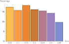
(a) $m=200$

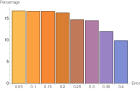
(b) $m=500$

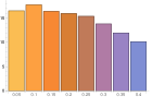
(c) $m=1000$

Figure 8: Percentage of data points whose geometric error can be bounded using Theorem C.3. These percentages were computed over noisy samples of 200, 500 and 1000 points, and are depicted respectively in the histograms.

Appendix D Optimization of Sampson Approximations

The constraint $C(\boldsymbol{z},\theta)$ typically depends not only on the measurements $\boldsymbol{z}$, but also some model parameters $\theta$ which we are estimating. Fitting the parameters we want to minimize the residuals for each measurement $\boldsymbol{z}_{k},~{}k=1,\dots,m$.

$$\theta^{\star}=\arg\min_{\theta}\sum_{k}\|\boldsymbol{J}_{k}^{\dagger}\boldsymbol{C}(\boldsymbol{z}_{k},\theta)\|^{2}$$ (99)

where $\boldsymbol{J}_{k}=\frac{\partial\boldsymbol{C}(\boldsymbol{z},\theta)}{\partial\boldsymbol{z}}\rvert_{\boldsymbol{z}=\boldsymbol{z}_{k}}$.

To apply standard non-linear least squares algorithms (e.g. Levenberg-Marquardt), we need to evaluate the Jacobian of the residuals $\boldsymbol{r}_{k}=\boldsymbol{J}_{k}^{\dagger}\boldsymbol{C}(\boldsymbol{z}_{k})$ w.r.t. $\theta$, i.e.

$$\frac{\partial\boldsymbol{r}_{k}}{\partial\theta} =\frac{\partial}{\partial\theta}\left((\frac{\partial\boldsymbol{C}}{\partial\boldsymbol{z}})^{\dagger}\boldsymbol{C}(\boldsymbol{z},\theta)\right)$$ (100)

$$=\left(\frac{\partial}{\partial\theta}(\frac{\partial\boldsymbol{C}}{\partial\boldsymbol{z}})^{\dagger}\right)\boldsymbol{C}(\boldsymbol{z},\theta)+(\frac{\partial\boldsymbol{C}}{\partial\boldsymbol{z}})^{\dagger}\frac{\partial\boldsymbol{C}}{\partial\theta}$$ (101)

Denote $\boldsymbol{J}_{\boldsymbol{z}}=\frac{\partial\boldsymbol{C}}{\partial\boldsymbol{z}}$ and $\boldsymbol{J}_{\theta}=\frac{\partial\boldsymbol{C}}{\partial\theta}$, then

$$\frac{\partial}{\partial\theta}\boldsymbol{J}_{\boldsymbol{z}}^{\dagger}=-\boldsymbol{J}_{\boldsymbol{z}}^{\dagger}\boldsymbol{J}_{\theta}\boldsymbol{J}_{\boldsymbol{z}}^{\dagger}+\boldsymbol{J}_{\boldsymbol{z}}^{\dagger}(\boldsymbol{J}_{\boldsymbol{z}}^{\dagger})^{T}\boldsymbol{J}_{\theta}(I-\boldsymbol{J}_{\boldsymbol{z}}\boldsymbol{J}_{\boldsymbol{z}}^{\dagger})$$ (102)

See Golub and Pereyra [7] for more details.

Appendix E Additional Experimental Results

In Table 6 we show the full per-scene results of the covariance aware camera pose refinement from Section 4.4 in the main paper, and Table 5 show the results of refining the vanishing points using both the mid-point error and the Sampson error. For this data there was no difference in the results of the refinement.

	YUB+[5]			NYU [18][12]
	Mean	AUC		Mean	AUC
VP from [19]	1.62	0.86		3.24	0.70
$\Lsh$ Mid-point	1.57	0.86		3.24	0.70
$\Lsh$ Sampson.	1.57	0.86		3.24	0.70

Table 5: Refinement of vanishing points.

$\tau$		Chess	Fire	Heads	Office	Pumpkin	Redkitchen	Stairs	Average
$5$px	Reproj.	0.86 / 2.47	0.84 / 2.11	0.75 / 1.07	0.89 / 3.05	1.24 / 4.78	1.39 / 4.15	1.22 / 4.44	1.03 / 3.20
	Reproj+Cov	0.85 / 2.45	0.82 / 2.04	0.74 / 1.02	0.87 / 2.99	1.22 / 4.75	1.36 / 4.03	1.15 / 4.28	1.01 / 3.10
	$\Lsh$ Sampson	0.85 / 2.45	0.82 / 2.04	0.74 / 1.02	0.87 / 2.99	1.22 / 4.74	1.36 / 4.02	1.14 / 4.27	1.01 / 3.10
$10$px	Reproj.	0.84 / 2.42	0.90 / 2.25	0.82 / 1.18	0.92 / 3.07	1.25 / 4.79	1.39 / 4.20	1.32 / 4.78	1.06 / 3.24
	Reproj+Cov	0.79 / 2.38	0.81 / 2.03	0.73 / 1.03	0.86 / 2.92	1.20 / 4.41	1.32 / 3.83	1.12 / 4.17	0.99 / 2.99
	$\Lsh$ Sampson	0.79 / 2.37	0.81 / 2.03	0.73 / 1.03	0.86 / 2.94	1.20 / 4.40	1.32 / 3.85	1.12 / 4.20	0.98 / 2.99
$20$px	Reproj.	0.87 / 2.53	1.08 / 2.72	1.04 / 1.45	1.06 / 3.43	1.38 / 5.41	1.49 / 4.50	1.99 / 6.84	1.21 / 3.63
	Reproj+Cov	0.75 / 2.30	0.80 / 2.06	0.73 / 1.03	0.88 / 2.91	1.13 / 4.30	1.29 / 3.81	1.36 / 4.89	0.99 / 3.00
	$\Lsh$ Sampson	0.75 / 2.31	0.80 / 2.07	0.73 / 1.03	0.88 / 2.92	1.13 / 4.34	1.29 / 3.88	1.44 / 5.25	1.00 / 3.02

Table 6: Full results for 7Scenes. Table shows the median rotation (deg.) and translation (cm) errors for each scene in the 7Scenes dataset for the experiment in Section 4.4 in the main paper.

References

- [1] Daniel Barath and Jiri Matas. Progressive-X: Efficient, anytime, multi-model fitting algorithm. In International Conference on Computer Vision (ICCV), 2019.
- [2] Paul Breiding and Sascha Timme. Homotopycontinuation.jl: A package for homotopy continuation in julia. In James H. Davenport, Manuel Kauers, George Labahn, and Josef Urban, editors, Mathematical Software – ICMS 2018, pages 458–465, Cham, 2018. Springer International Publishing.
- [3] Wojciech Chojnacki, Michael J. Brooks, Anton Van Den Hengel, and Darren Gawley. On the fitting of surfaces to data with covariances. IEEE Trans. Pattern Analysis and Machine Intelligence (PAMI), 2000.
- [4] Ondřej Chum, Tomáš Pajdla, and Peter Sturm. The geometric error for homographies. Computer Vision and Image Understanding (CVIU), 2005.
- [5] Patrick Denis, James H Elder, and Francisco J Estrada. Efficient edge-based methods for estimating manhattan frames in urban imagery. In European Conference on Computer Vision (ECCV), 2008.
- [6] Jan Draisma, Emil Horobeţ, Giorgio Ottaviani, Bernd Sturmfels, and Rekha R Thomas. The euclidean distance degree of an algebraic variety. Foundations of computational mathematics, 16:99–149, 2016.
- [7] Gene H Golub and Victor Pereyra. The differentiation of pseudo-inverses and nonlinear least squares problems whose variables separate. SIAM Journal on numerical analysis, 10(2):413–432, 1973.
- [8] Richard Hartley and Andrew Zisserman. Multiple view geometry in computer vision. Cambridge university press, 2003.
- [9] Richard I Hartley and Peter Sturm. Triangulation. Computer Vision and Image Understanding (CVIU), 1997.
- [10] Allen Hatcher. Algebraic topology. Cambridge University Press, 2005.
- [11] Yuhe Jin, Dmytro Mishkin, Anastasiia Mishchuk, Jiri Matas, Pascal Fua, Kwang Moo Yi, and Eduard Trulls. Image Matching Across Wide Baselines: From Paper to Practice. International Journal of Computer Vision (IJCV), 129(2):517–547, Feb. 2021.
- [12] Florian Kluger, Eric Brachmann, Hanno Ackermann, Carsten Rother, Michael Ying Yang, and Bodo Rosenhahn. CONSAC: Robust multi-model fitting by conditional sample consensus. In Computer Vision and Pattern Recognition (CVPR), 2020.
- [13] Viktor Larsson, Kalle Astrom, and Magnus Oskarsson. Efficient solvers for minimal problems by syzygy-based reduction. In Computer Vision and Pattern Recognition (CVPR), 2017.
- [14] Spyridon Leonardos, Roberto Tron, and Kostas Daniilidis. A metric parametrization for trifocal tensors with non-colinear pinholes. In Computer Vision and Pattern Recognition (CVPR), 2015.
- [15] Peter Lindstrom. Triangulation made easy. In Computer Vision and Pattern Recognition (CVPR), 2010.
- [16] Quan-Tuan Luong and Olivier D Faugeras. The fundamental matrix: Theory, algorithms, and stability analysis. International Journal of Computer Vision (IJCV), 1996.
- [17] Laurentiu G Maxim, Jose I Rodriguez, and Botong Wang. Euclidean distance degree of the multiview variety. SIAM Journal on Applied Algebra and Geometry, 4(1):28–48, 2020.
- [18] Pushmeet Kohli Nathan Silberman, Derek Hoiem and Rob Fergus. Indoor segmentation and support inference from rgbd images. In European Conference on Computer Vision (ECCV), 2012.
- [19] Rémi Pautrat, Daniel Barath, Viktor Larsson, Martin R Oswald, and Marc Pollefeys. Deeplsd: Line segment detection and refinement with deep image gradients. In Computer Vision and Pattern Recognition (CVPR), 2023.
- [20] Felix Rydell, Elima Shehu, and Angelica Torres. Theoretical and numerical analysis of 3d reconstruction using point and line incidences. arXiv preprint arXiv:2303.13593, 2023.
- [21] Paul D Sampson. Fitting conic sections to “very scattered” data: An iterative refinement of the bookstein algorithm. Computer graphics and image processing, 1982.
- [22] Paul-Edouard Sarlin, Cesar Cadena, Roland Siegwart, and Marcin Dymczyk. From coarse to fine: Robust hierarchical localization at large scale. In Computer Vision and Pattern Recognition (CVPR), 2019.
- [23] Jamie Shotton, Ben Glocker, Christopher Zach, Shahram Izadi, Antonio Criminisi, and Andrew Fitzgibbon. Scene coordinate regression forests for camera relocalization in RGB-D images. In Computer Vision and Pattern Recognition (CVPR), 2013.
- [24] Peter Sturm. Vision 3D non calibrée: contributions à la reconstruction projective et étude des mouvements critiques pour l’auto-calibrage. PhD thesis, Institut National Polytechnique de Grenoble-INPG, 1997.
- [25] Zygmunt L Szpak, Wojciech Chojnacki, and Anton Van Den Hengel. Guaranteed ellipse fitting with the sampson distance. In European Conference on Computer Vision (ECCV), 2012.
- [26] Gabriel Taubin. Estimation of planar curves, surfaces, and nonplanar space curves defined by implicit equations with applications to edge and range image segmentation. IEEE Trans. Pattern Analysis and Machine Intelligence (PAMI), 1991.
- [27] Mikhail Terekhov and Viktor Larsson. Tangent sampson error: Fast approximate two-view reprojection error for central camera models. In International Conference on Computer Vision (ICCV), 2023.