Abstract

An Event-Related Potential (ERP)-based Brain-Computer Interface (BCI) Speller System assists people with disabilities communicate by decoding electroencephalogram (EEG) signals. A P300-ERP embedded in EEG signals arises in response to a rare, but relevant event (target) among a series of irrelevant events (non-target). Different machine learning methods have constructed binary classifiers to detect target events, known as calibration. Existing calibration strategy only uses data from participants themselves with lengthy training time, causing biased P300 estimation and decreasing prediction accuracy. To resolve this issue, we propose a Bayesian signal matching (BSM) framework for calibrating the EEG signals from a new participant using data from source participants. BSM specifies the joint distribution of stimulus-specific EEG signals among source participants via a Bayesian hierarchical mixture model. We apply the inference strategy: if source and new participants are similar, they share the same set of model parameters, otherwise, they keep their own sets of model parameters; we predict on the testing data using parameters of the baseline cluster directly. Our hierarchical framework can be generalized to other base classifiers with clear likelihood specifications. We demonstrate the advantages of BSM using simulations and focus on the real data analysis among participants with neuro-degenerative diseases.

Keywords: Bayesian Method, Mixture Model, Data Integration, P300, Brain-Computer Interface, Calibration-Less Framework.

1 Introduction

1.1 Background

A Brain-Computer Interface (BCI) is a device that interprets brain activity to assist people with severe neuro-muscular diseases with normal communications. An electroencephalogram (EEG)-based BCI speller system is one of the most popular BCI applications, which enables a person to “type” words without using a physical keyboard by decoding the recorded EEG signals. The EEG brain activity has the advantages of non-invasiveness, low cost, and high temporal resolution (Niedermeyer and da Silva,, 2005).

The P300 event-related potential (ERP) BCI design, known as the P300 ERP-BCI design (Donchin et al.,, 2000), is one of the most widely used BCI frameworks and the focus of this manuscript. However, other types of ERPs exist that help interpret and classify brain activity. An ERP is a signal pattern in the EEG signals in response to an external event. The P300 ERP is a particular ERP that occurs in response to a rare, but relevant event (i.e., highlighting a group of characters on the screen) among a group of frequent, but irrelevant ones. The relevant (target) P300 ERP usually has a positive deflection in voltage with the latency (the time intervals between the onset of the event and the first response peak) around 300 ms.

Under the P300 ERP-BCI design, participants wore an EEG cap, sat next to a virtual screen, and focused on a specific character to spell, denoted as the “target character.” The study applied the row-and-column paradigm (RCP) developed by (Farwell and Donchin,, 1988), which is a 6 $\times$ 6 grid of characters. Each event is either a row stimulus or a column stimulus. The order of rows and columns is random, but loops through all rows and columns every consecutive 12 stimuli, known as a sequence. Participants were asked to mentally count whenever they saw a row or column stimulus containing the target character or to do nothing. Thus, within each sequence, there were always exactly two stimuli that were supposed to elicit target P300 ERPs.

The fundamental operation of the P300 ERP-BCI design is that it presents a sequence of stimuli on a virtual keyboard and that it analyzes the EEG signals in a fixed time response window post event to make a binary decision whether the participant’s brain elicits a target P300 ERP response. After each method produces binary classifier scores for each stimulus, those scores are converted into character-level probabilities. Finally, the character with the highest probability is shown on the virtual screen. Many machine learning (ML) methods have successfully constructed such binary classifiers for P300 ERPs, including stepwise linear discriminant analysis (swLDA) (Donchin et al.,, 2000), (Krusienski et al.,, 2008), support vector machine (SVM) (Kaper et al.,, 2004), independent component analysis (ICA) (Xu et al.,, 2004), linear discriminant analysis (LDA) with xDAWN filter (Rivet et al.,, 2009), convolutional neural network (CNN) (Cecotti and Graser,, 2010), and Riemannian geometry (Barachant et al.,, 2011). These methods usually concatenate multi-channel EEG signals without considering spatial dependency. Here, an EEG channel refers to an electrode placed on the scalp to achieve stable prediction accuracy. Finally, Ma et al., (2022) attempted to improve prediction accuracy and identify spatial-temporal discrepancies between target and non-target P300 responses from the generative perspective. The method also explicitly addressed the overlapping ERP issue directly.

1.2 Challenge and Existing Work

Before participants performed the free-typing sessions, they usually copied a multi-character phrase to build a participant-specific training profile. We referred to the previous two procedures as testing and calibration, respectively. Since the signal-to-noise ratio (SNR) of EEG signals was generally low, current calibration strategy simply collected data from participants themselves with a fixed but large amount of sequence replications. However, a lengthy calibration procedure might cause attention shift and mental fatigue. Participants tended to feel bored and might elicit biased target P300 ERPs, which made the calibration process inaccurate and inefficient. Therefore, the challenge became how to reduce participants’ calibration time with decent prediction accuracy for the free-typing sessions. Existing work has tackled this problem by applying the idea of transfer learning, which was originally introduced by Bozinovski and Fulgosi, in 1976, that information was extracted and stored from existing problems to solve a new but similar problem. In statistical fields, we denoted this concept as data integration (Lenzerini,, 2002). To avoid confusion, we do not distinguish among “transfer learning”, “data integration”, or “borrowing” in our study.

This subsection briefly introduces existing works that have explored the transfer learning under different domains for information leveraging with applications to P300 ERP-BCIs. A recent review (Wu et al.,, 2020) on transfer learning summarized methods between 2016 and 2020 with six paradigms and applications. For P300-ERP BCI paradigm, they considered cross-session/participant and cross-device transfer learning scenarios and produced a nice table for alignment-related approaches including offline/online status, known/unknown labels, alignment framework, referencing objects, base classifiers, and computational costs. We will continue introducing the work that were not covered previously.

First, ensembles was an intuitive idea to incorporate data from other domains that combined the results of different classifiers within the same training set. Each classifier made predictions on a test set, and the results were combined with a voting process. Rakotomamonjy and Guigue, in 2008 and Johnson and Krusienski, in 2009 were the first to apply the ensemble method to P300 ERP-BCIs by averaging the outputs of multiple SVMs and swLDAs, respectively, where base binary classifier was trained on a small part of the available data. Völker et al., in 2018 and Onishi, in 2020 applied the ensemble method by averaging the outputs of multiple CNNs to visual and auditory P300 ERP-BCI datasets, respectively. Onishi and Natsume, also mentioned that ensemble methods with overlapping partitioning criterion yielded better prediction performance than the ensemble methods with a naive partitioning criterion.

As an alternative solution, Xu et al., in 2015 proposed the Ensemble Learning Generic Information (ELGI), which combined the data of the new participant with the data of source participants to form a hybrid ensemble. They split the data of each source participant into target and non-target subsets. They applied the swLDA method to construct the base classifiers by combining different subsets as follows: the target and non-target subsets from the new participant, the target subset from the new participant and the non-target subset from each source participant, and the target subset from each source participant and the non-target subset from the new participant. Thus, the resulting ensemble had $(2N+1)$ base classifiers, where $N$ is the number of source participants. They further introduced the Weighted Ensemble Learning Generic Information (WELGI) (Xu et al.,, 2016) by adding weights to each base classifier. Similarly, An et al., in 2020 proposed a weighted participant-semi-independent classification method (WSSICM) for P300 ERP-based BCIs, where they used the SVM method as the base classifier. The base classifier was fit by combining the entire data of each source participant and a small portion of data of the new participant. An ad-hoc approach was applied to determine the weighted coefficients of base classifiers for participant selection. Likewise, Adair et al., in 2017 proposed the Evolved Ensemble Learning Generic Information (eELGI). The authors argued that grouping training sets by participants was not an optimal selection criterion. Instead, they developed an evolutionary algorithm by permuting datasets among source participants to form the base classifiers, which were constructed using the swLDA method.

Finally, Riemannian geometry has gained increasing attention recently due to its fast speed to converge and a natural framework to leverage information from source participants. The Riemannian geometry classifier was originally proposed by Barachant et al., in 2011. The input data for Riemannian geometry were the sample covariance matrices. The distance-based algorithm based on the Riemannian geometry was called Minimum Distance to Mean (MDM). Instead of computing the Euclidean distance between EEG signals within the Euclidean space, the MDM method computed the Riemmanian distance between sample covariance matrices on the Riemannian manifold, and predicted the class label of which “mean” covariance matrix was the closest to the new covariance matrix with respect to the Riemmannian distance. Additional studies adapted the MDM classifier to the P300 ERP-BCI design by augmenting the covariance matrix with the label-specific reference signal patterns (Congedo et al.,, 2013), (Barachant and Congedo,, 2014). This modified classifier was a combination of first- and second-order statistics and compensated for the loss of the temporal structure information with the referencing signal components.

Recent studies have shown a growing interest in building the transfer learning with the Riemannian geometry. For example, Rodrigues et al., in 2018 presented a transfer learning approach to tackle the heterogeneity of EEG signals across different sessions or participants using the Riemannian procrustes analysis (RPA). Before the authors applied the MDM classifier, they applied certain affine transformations to raw participant-level covariance matrices such that the resulting covariance matrices were less heterogeneous across sessions or participants while their Riemannian distances were preserved. Li et al., in 2020 also standardized the covariance matrices across participants by applying the affine transformation with the participant-specific Riemannian geometric mean covariance matrix. Finally, Khazem et al., in 2021 proposed another transfer learning approach, denoted as Minimum Distance to Weighted Mean (MDWM). They combined estimated mean covariance matrices from source participants and the new participant by the definition of Riemannian distance. They controlled the trade-off between new and source contribution by the power parameter, but they treated them as a hyper-parameter and did not estimate it during the calibration session. Although these three methods shared the idea that they applied different transformations to the borrowed data so that the covariance matrices were robust to aggregate information from source participants, Khazem et al., emphasized that further improvement in prediction accuracy could benefit from a proper selection of source participants.

1.3 Our Contributions

To reduce the calibration time while maintaining similar prediction accuracy, we propose a Bayesian Signal Matching (BSM) method to build a participant-dependent, calibration-less framework. BSM reduces the calibration time of a new participant by borrowing data from pre-existing source participants’ pool. Instead of transforming and homogenizing source calibration data and selecting on the level of stimuli, we simply borrow data on the level of participants, which is an intuitive clustering criterion. BSM specifies the joint distribution of stimulus-specific EEG signals from all participants via a Bayesian hierarchical mixture model. Our method has advantages from both inference and prediction perspectives. First, unlike the conventional clustering approach, we specify the baseline cluster as the one that matches the new participant. The selection indicators indicates how close source calibration data resemble the new data on the level of participants. If the selection indicator is 1, we merge source participant’s data with the new participant’s data, otherwise, we keep the source participant’s data as a separate cluster. Second, we use the baseline cluster to predict on the testing data directly without refitting the model with the augmented data. Finally, our proposed hierarchical framework is flexible to generalize to other classifiers with specific likelihood specifications.

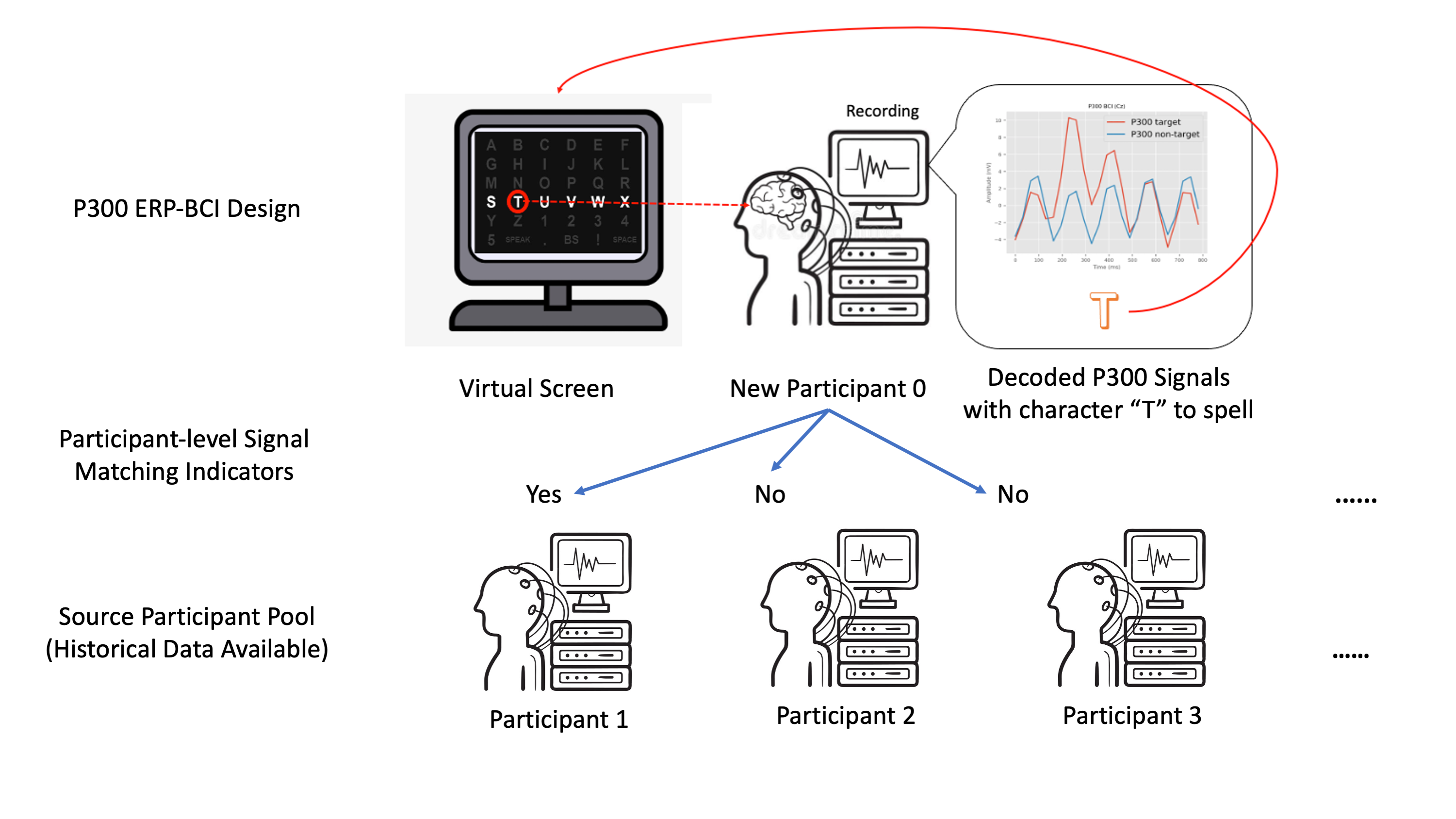
Figure 1: An illustration of proposed data integration framework. Given rich and known data from the source participants $1,2,3,\cdots$ and a small amount of training data from the new participant 0, we construct the BSM binary classifier, apply it to the free-typing datasets and convert binary classification scores to character-level probabilities with participant-specific selection indicators that demonstrates the similarity of signals between source participants and participant $0$.

The paper is organized as follows: Section 2 presents the framework for the Bayesian hierarchical mixture model using the generative parametric form as the base classifier. Section 3 introduces the details for posterior inference. Sections 4 and 5 present the numerical results for simulation and real data analysis, respectively. Section 6 concludes the paper with a discussion.

2 Methods

2.1 Basic Notations and Problem Setup

Let $\mathcal{MVN}(\bm{\mu},\Sigma)$ be a multivariate normal distribution with mean and covariance matrix parameters $\bm{\mu}$ and $\Sigma$. Let $\mathcal{MN}(M,U,V)$ be a matrix normal distribution with location matrix $M$ and two scale matrix parameters $U$ and $V$ (Dawid,, 1981). Let $\mathrm{Diag}(\cdot)$ be a diagonal matrix notation. Let $\mathcal{LN}(\mu,\sigma)$ be a Log-Normal distribution with mean and scale parameters $\mu$ and $\sigma$. Let $\mathcal{HC}(x_{0},\sigma)$ be a Half-Cauchy distribution with location and scale parameters $x_{0}$ and $\sigma$. Let $\mathcal{U}(a,b)$ be a Uniform distribution with lower and upper bounds $a$ and $b$.

Let $n=0,\ldots,N$ be the participant index, where $n=0$ refers to the new participant and $n=1,\ldots,N$ refer to source participants. Let $l=1,\ldots,L_{n}$ and $i=1,\ldots,I_{n}$ be the character index and sequence index for participant $n$, respectively. We follow the conventional RCP design such that each sequence contains $J(J=12)$ stimuli, including six row stimuli from top to bottom $(1,\ldots,6)$ and six column stimuli from left to right $(7,\ldots,12)$ on the $6\times 6$ virtual keyboard (See the virtual screen in Figure 1). For the $i$th sequence, $l$th target character, and $n$th participant, let $\bm{W}_{n,l,i}=(W_{n,l,i,1},\ldots,W_{n,l,i,12})^{\top}$ be a stimulus code indicator that takes values from the permutation of $\{1,\ldots,12\}$. Under the RCP design, given the target character and the stimulus-code indicators, there are exactly two target stimuli and ten non-target stimuli within each sequence. We define $\bm{Y}_{n,l,i}=(Y_{n,l,i,1},\ldots,Y_{n,l,i,12})^{\top}$ as the stimulus-type indicator for the $i$th sequence, $l$th target character, and $n$th participant, where $Y_{n,l,i,j}\in\{0,1\}$. For example, given a target character “T” and a stimulus code indicator $\bm{W}_{n,l,i}=(7,9,10,5,1,2,8,11,6,4,3,12)^{\top}$, we obtain its stimulus type indicator $\bm{Y}_{n,l,i}=(0,0,0,0,0,0,1,0,0,1,0,0)^{\top}$, where the indices of $1$s correspond to the indices of the $4$th row and $2$nd column (denoted by $8$) in $\bm{W}_{n,l,i}$. Let $k=0,\ldots,K-1$ be the cluster index, where $k=0$ is the cluster that matches the new participant and $k=1,\ldots,K-1$ are the clusters within source participants. Finally, we incorporate $E$ channels of EEG signals and let $e(e=1,\ldots,E)$ be the channel index. We extract channel-specific EEG segments from the onset of each stimulus with a long EEG response window length (with $T_{0}$ time points). We denote $\bm{X}_{n,l,i,j,e}(s)$ as the extracted EEG signal segment of the $j$th stimulus, $i$th sequence, $l$th target character, and $n$th participant from channel $e$ at time $s\in[0,s_{T_{0}}]$.

2.2 A Bayesian Signal Matching Clustering Framework

Given sufficient training data from the source participants and a small amount of training data from the new participant, our primary goal is to reduce calibration time by integrating a proper subset of training data on the level of source participants into the augmented training data for the new participant. We made three assumptions to simplify the model representation as follows: First, we let all source participants spell the same character $\omega$ with the same sequence replication size $I$, so we drop the target character index $l$ and the source participant index $n$ from $I_{n}$. Second, we assumed that target and non-target ERP functions shared the same covariance matrix within the same cluster. Finally, we performed selection with respect to the target ERP data and we excluded non-target ERP data from the source participants’ pool. Figure 1 provides a detailed illustration of the data integration framework of proposed Bayesian signal matching method.

For the new participant, i.e., when $n=0$, we assume

$$\bm{X}_{0,i,j}=\bm{B}_{0,1}Y_{0,i,j}+\bm{B}_{0,0}(1-Y_{0,i,j})+\bm{\epsilon}_{0,i,j},$$ (1)

where $\bm{B}_{0,1},\bm{B}_{0,0}$, and $\bm{\epsilon}_{0,i,j}$ are target ERP matrix, non-target ERP matrix, and random noise matrix of the new participant, of the same size $T_{0}\times E$, respectively. For source participant $n,n>0$, we introduce a participant-specific binary indicator $Z_{n}\in\{0,1\}$ and assume that

$$\operatorname{Pr}(Z_{n}=1)=\pi_{n},\\$$ (2)

where $\pi_{n}$ is the probability whether source participant $n$ matches the new participant. With $\{Z_{n}\}$, we consider a signal matching model for the EEG signal matrix for source participant $n$ as follows:

$$\quad\quad\quad\quad\quad\bm{X}_{n,i,j}=\{\bm{B}_{0,1}Y_{n,i,j}+\bm{B}_{0,0}(1-Y_{n,i,j})\}Z_{n}\\ +\{\bm{B}_{n,1}Y_{n,i,j}+\bm{B}_{n,0}(1-Y_{n,i,j})\}(1-Z_{n})+\bm{\epsilon}_{n,i,j},\quad\quad\quad$$ (3)

where $\bm{B}_{n,1},\bm{B}_{n,0}$, and $\bm{\epsilon}_{n,i,j}$ are target ERP matrix, non-target ERP matrix, and stimulus-specific random error matrix of source participant $n$, of the same size $T_{0}\times E$, respectively. Of note, (2) and (3) assume that each source participant has either has the new participant’s parameter set or their own parameter set. However, we do not borrow non-target EEG data of source participants for making statistical inferences. All $\bm{X}_{n,i,j},\bm{B}_{n,1}$, $\bm{B}_{0,0}$, and $\bm{\epsilon}_{n,i,j}$ are matrices with the same size of $E$ by $T_{0}$.

For random error matrix $\bm{\epsilon}_{n,i,j}$, where $n\in\{0,1,\cdots,N\}$, we assume an additive relationship to characterize its spatial-temporal error structure.

$$\bm{\epsilon}_{n,i,j} =\bm{\xi}_{n,i,j}+\bm{\varepsilon}_{n,i,j},$$ (4)

$$\bm{\xi}_{n,i,j} =(\bm{\xi}_{n,i,j,1},\cdots,\bm{\xi}_{n,i,j,T_{0}})^{\top},$$

$$\bm{\varepsilon}_{n,i,j} =(\bm{\varepsilon}_{n,i,j,1},\cdots,\bm{\varepsilon}_{n,i,j,E}),$$

where $\bm{\xi}_{n,i,j,t},(t=1,\cdots,T_{0})$ is a vector of spatial random effects for $E$ channels at time point $t$, and $\bm{\varepsilon}_{n,i,j,e},(e=1,\cdots,E)$ is a vector of temporal random effects for $T_{0}$ time points of channel $e$. Let $\bm{\Sigma}_{n}^{s}=\bm{V}_{n}\bm{R}_{n}^{s}\bm{V}_{n}^{\top}$, $\bm{R}_{n}^{s}$, and $\bm{R}_{n}^{t}$ be the spatial covariance matrix, spatial correlation matrix, and temporal correlation matrix for participant $n,n\in\{0,...,N\}$, respectively. $\bm{R}_{n}^{s}$ is a correlation matrix with the structure of compound symmetry characterized by a scale parameter $\eta_{n}\in(0,1)$; $\bm{V}_{k}$ is a diagonal matrix characterized by $(\sigma_{n,1},\cdots,\sigma_{\sigma_{n,E}})$, and $\bm{R}_{k}^{t}$ is a correlation matrix with the structure of exponential decay characterized by a scalar parameter $\rho_{n}\in(0,1)$. Given $Z_{n}=1$, where $n\in\{1,\cdots,N\}$ we assume that $\bm{\xi}_{n,i,j,t}$ and $\bm{\varepsilon}_{n,i,j,e}$ follow multivariate normal distributions with zero mean vectors and covariance matrices of the new participant; given $Z_{n}=0$, we assume that $\bm{\xi}_{n,i,j,t}$ and $\bm{\varepsilon}_{n,i,j,e}$ follow multivariate normal distributions with zero mean vectors and participant-specific covariance matrices. In summary,

$$(\bm{\xi}_{n,i,j,t}\mid Z_{n}) \sim\mathcal{MVN}\{\bm{0},\bm{\Sigma}_{0}^{s}Z_{n}+\bm{\Sigma}_{n}^{s}(1-Z_{n})\},$$ (5)

$$(\bm{\varepsilon}_{n,i,j,e}\mid Z_{n}) \sim\mathcal{MVN}\{\bm{0},\bm{R}_{0}^{t}Z_{n}+\bm{R}_{n}^{t}(1-Z_{n})\}.$$

Let $\bm{\Theta}$ be a collection of all unknown parameters, where the primary parameters of interest are those associated with the new participant, i.e., $\bm{B}_{0,1},\bm{B}_{0,0},\sigma_{0,e}^{2},\eta_{0}$, and $\rho_{0}$. We are also interested in making inferences on the posterior probability of matching the new participant, i.e., $\operatorname{Pr}(Z_{n}=1\mid\bm{X},\bm{Y})$, for source participant $n$. The remaining parameters are considered as nuisance parameters.

3 Posterior Inferences

3.1 Model Reparametrization and Prior Specifications

We rewrite the model by applying the notation of matrix normal distribution

$$\bm{X}_{0,i,j}\mid Y_{0,i,j}=1;\bm{\Theta} \sim\mathcal{MN}(\bm{B}_{0,1},\bm{\Sigma}_{0}^{s},\bm{R}_{0}^{t}),$$ (6)

$$\bm{X}_{0,i,j}\mid Y_{0,i,j}=0;\bm{\Theta} \sim\mathcal{MN}(\bm{B}_{0,0},\bm{\Sigma}_{0}^{s},\bm{R}_{0}^{t}),$$

$$\bm{X}_{n,i,j}\mid Z_{n},Y_{n,i,j}=1;\bm{\Theta} \sim\mathcal{MN}\{\bm{B}_{0,1}Z_{n}+\bm{B}_{n,1}(1-Z_{n}),$$

$$\quad\quad\quad\quad\bm{\Sigma}_{0}^{s}Z_{n}+\bm{\Sigma}_{n}^{s}(1-Z_{n}),$$

$$\quad\quad\quad\quad\bm{R}_{0}^{t}Z_{n}+\bm{R}_{n}^{t}(1-Z_{n})\},\quad n>0,$$

where $\bm{B}_{n,1}=(\bm{\beta}_{n,1,1}^{\top},\cdots,\bm{\beta}_{n,1,E}^{\top})$ and $\bm{B}_{0,0}=(\bm{\beta}_{0,0,1}^{\top},\cdots,\bm{\beta}_{0,0,E}^{\top})$.

To better characterize the multi-channel ERP response functions $\{\bm{B}_{n,1}\}_{n=0}^{N}$ and $\bm{B}_{0,0}$, we frame them using the notation of a multivariate Gaussian process. First, we adopt the definition (Dixon and Crepey,, 2018) to define a multivariate Gaussian processes as follows: Let $\bm{\mu}:\mathbb{R}\rightarrow\mathbb{R}^{E}$, $\kappa:\mathbb{R}\times\mathbb{R}\rightarrow\mathbb{R}$, $\bm{\Omega}\in\mathbb{R}^{E\times E}$, and $\{s_{t}\}_{t=1}^{T_{0}}$ be a vector-valued mean function, a kernel on the temporal domain, a positive definite parameter covariance matrix on the spatial domain, and input points, respectively. Here, the general multidimensional input vector is reduced to the scalar indexed by time only. $\bm{f}$ is a multivariate Gaussian process on $\mathbb{R}$ with vector-valued mean function $\bm{\mu}$, kernel $\kappa$, and row covariance matrix $\bm{\Omega}$ if the vectorization of any finite collection of vector-valued variables have a joint multivariate Gaussian distribution, i.e.,

$$\operatorname{vec}\left\{\left[\bm{f}(s_{1}),\cdots,\bm{f}(s_{T_{0}})\right]\right\}\sim\mathcal{MVN}\left(\operatorname{vec}\left(\bm{M}\right),\bm{\Sigma}\otimes\bm{\Omega}\right),$$ (7)

where $\bm{f},\bm{\mu}\in\mathbb{R}^{E}$ are column vectors whose components are the functions $\{\bm{f}_{e}\}_{e=1}^{E}$ and $\{\bm{\mu}_{e}\}_{e=1}^{E}$, respectively. Furthermore, $\bm{M}\in\mathbb{R}^{E\times T_{0}}$ with $\bm{M}_{e,t}=\bm{\mu}_{e}(s_{t})$, $\bm{\Sigma}\in\mathbb{R}^{T_{0}\times T_{0}}$ with $\bm{\Sigma}_{t_{1},t_{2}}=k(s_{t_{1}},s_{t_{2}})$, where $t_{1},t_{2}\in\mathbb{Z}$ and $0\leq t_{1},t_{2}\leq T_{0}$, and $\otimes$ is the Kronecker product operator. We denote $\bm{f}\sim\mathcal{MGP}(\bm{\mu},\kappa,\bm{\Omega})$.

In our case, we let $\bm{b}_{n,1}$ be an $E$-dim target ERP function of participant $n$ characterized by $\bm{\mu}_{n,1},\kappa_{1},\bm{\Sigma}_{n}^{s}$, $n=0,\cdots,N$, and $\bm{b}_{0,0}$ be another $E$-dim non-target ERP function of participant $0$ characterized by $\bm{\mu}_{0,0},\kappa_{0},\bm{\Sigma}_{0}^{s}$. To simplify, we let $\bm{\mu}_{n,1}=\bm{\mu}_{0,0}=\bm{0}$ and apply a $\gamma$-exponential kernel function to specify target kernel $\kappa_{1}$ and non-target kernel $\kappa_{0}$ as follows:

$$k(z_{i},z_{j})=\psi_{0}\exp\left\{-\left(\frac{||z_{i}-z_{j}||_{2}^{2}}{s_{0}}\right)^{\gamma_{0}}\right\},$$ (8)

where $0\leq\gamma_{0}<2,s_{0}>0$. In practice, $\gamma_{0}$ and $s_{0}$ are treated as hyper-parameters and selected among a group of values and we do not further differentiate among participants. For participant-specific kernel variance parameters $\psi_{n,1}$ and $\psi_{0,0}$, we assign Log-Normal priors with the a mean zero and a scale one. In addition, we define a function $\phi(\cdot)$ as an eigenfunction of kernel $k$ with eigenvalue $\lambda$ if it satisfies the following integral:

$$\int k(s,s^{\prime})\phi(s)ds=\lambda\phi(s^{\prime}).$$

In general, the number of eigenfunctions is infinite, i.e., $\{\phi_{l}(s)\}_{l=1}^{+\infty}$, and we rank them by the descending order of their corresponding eigenvalues $\{\lambda_{l}\}_{l=1}^{+\infty}$. The Mercer’s Theorem suggests that the kernel function $k$ can be decomposed as a weighted summation of normalized eigenfunctions $\phi_{l}(s)$ with positive eigenvalues $\lambda_{l}$ and approximated with a sufficient large $L$ subgroup as follows:

$$k(s,s^{\prime})=\sum_{l=1}^{+\infty}\lambda_{l}\phi_{l}(s)\phi_{l}(s^{\prime})\approx\sum_{l=1}^{L}\lambda_{l}\phi_{l}(s)\phi_{l}(s^{\prime})$$

Thus, a random function $\bm{f}$ can be represented as a linear combination of the above eigenfunctions and approximated with a sufficient large $L$ subgroup evaluated at $s$ as follows:

$$\bm{f}(s) =\begin{pmatrix}f_{1}(s)\\ \vdots\\ f_{e}(s)\\ \vdots\\ f_{E}(s)\\ \end{pmatrix}=\begin{pmatrix}\sum_{l=1}^{\infty}a_{1,l}\phi_{l}(s)\\ \vdots\\ \sum_{l=1}^{\infty}a_{e,l}\phi_{l}(s)\\ \vdots\\ \sum_{l=1}^{\infty}a_{E,l}\phi_{l}(s)\\ \end{pmatrix}\approx\begin{pmatrix}\sum_{l=1}^{L}a_{1,l}\phi_{l}(s)\\ \vdots\\ \sum_{l=1}^{L}a_{e,l}\phi_{l}(s)\\ \vdots\\ \sum_{l=1}^{L}a_{E,l}\phi_{l}(s)\\ \end{pmatrix},$$

where $(a_{1,l},\cdots,a_{E,l})^{\top}\sim\mathcal{MVN}(\bm{0},\bm{\Omega}),l>0$. For participant-and-channel-specific noise variance parameters $\sigma_{n,e}^{2}$, we assign Half-Cauchy priors with a mean zero and a scale five. For temporal and spatial parameters $\rho_{n}$ and $\eta_{n}$, we assign discrete uniform priors among a grid of candidate values between 0 and 1. Finally, the prior specifications are summarized as follows:

$$\bm{b}_{n,1}(s)\sim\mathcal{MGP}(\bm{0},\psi_{n,1}\kappa_{1},\bm{\Sigma}_{n}^{s}),\quad\bm{b}_{0,0}(s)\sim\mathcal{MGP}(\bm{0},\psi_{0,0}\kappa_{0},\bm{\Sigma}_{0}^{s}),$$ (9)

$$\psi_{n,1},\psi_{0,0}\overset{\mathrm{indep.}}{\sim}\mathcal{LN}(0,1),$$

$$\sigma_{n,e}\sim\mathcal{HC}(0,5.0),\quad\rho_{n}\sim\mathcal{U}(0,1),\quad\eta_{n}\sim\mathcal{U}(0,1),$$

$$\mathrm{for} n=0,\cdots,N,\quad e=1,\cdots,E,$$

3.2 Markov Chain Monte Carlo

We apply the Gibbs Sampling method to estimate random functions $\bm{b}_{n,1},\bm{b}_{0,0}$ and covariance-related parameters $\sigma_{n,e}^{2},\rho_{n}$, and $\eta_{n}$. By Mercer’s representation theorem, we obtain that

$$\bm{b}_{n,1}(s) =\psi_{n,1}\sum_{l=1}^{+\infty}\operatorname{Diag}(\bm{a}_{n,1,l})\phi_{1,l}(s)\approx\psi_{n,1}\sum_{l=1}^{L_{1}}\operatorname{Diag}(\bm{a}_{n,1,l})\phi_{1,l}(s),\quad n=0,\cdots,N,$$ (10)

$$\bm{b}_{0,0}(s) =\psi_{0,0}\sum_{l=1}^{+\infty}\operatorname{Diag}(\bm{a}_{0,0,l})\phi_{0,l}(s)\approx\psi_{0,0}\sum_{l=1}^{L_{0}}\operatorname{Diag}(\bm{a}_{0,0,l})\phi_{0,l}(s),$$

where $\{\bm{a}_{n,1,l}\}_{n=0}^{N}$ and $\bm{a}_{0,0,l}$ are column vectors of coefficient parameters associated with eigenfunctions $\phi_{1,l}$ and $\phi_{0,l}$, respectively. We evaluate $\bm{b}_{n,1}(s)$ and $\bm{b}_{0,0}(s)$ over a group of input time points $\{s_{t}\}_{t=1}^{T_{0}}$ and define them $\bm{B}_{n,1}$ and $\bm{B}_{0,0}$, respectively. Then, we adopt Eq (8) to calculate the kernel covariances $\bm{\Psi}_{1}$ and $\bm{\Psi}_{0}$ associated with kernel function $\kappa_{1}$ and $\kappa_{0}$, respectively. $\bm{B}_{n,1}$ and $\bm{B}_{0,0}$ can be approximated by

$$\bm{B}_{n,1} \approx\psi_{n,1}\cdot\bm{A}_{n,1}\bm{\Psi}_{1}^{1:L_{1}},\quad\bm{A}_{n,1}=\left(\bm{a}_{n,1,1}\cdots\bm{a}_{n,1,l}\cdots\bm{a}_{n,1,L_{1}}\right),\quad n\in\{0,\cdots,N\},$$ (11)

$$\bm{B}_{0,0} \approx\psi_{0,0}\cdot\bm{A}_{0,0}\bm{\Psi}_{0}^{1:L_{0}},\quad\bm{A}_{0,0}=\left(\bm{a}_{0,0,1}\cdots\bm{a}_{0,0,l}\cdots\bm{a}_{0,0,L_{0}}\right),$$

$$\bm{A}_{n,1} \sim\mathcal{MN}\left(\bm{0},\bm{\Sigma}_{n}^{s},\bm{V}_{\bm{\Psi}_{1}}^{1:L_{1}}\right),\quad\bm{A}_{0,0}\sim\mathcal{MN}\left(\bm{0},\bm{\Sigma}_{0}^{s},\bm{V}_{\bm{\Psi}_{0}}^{1:L_{0}}\right),$$

where $\bm{A}_{n,1}$ and $\bm{A}_{0,0}$ follow matrix normal prior distributions with closed posterior forms (Zhang et al.,, 2021), and $\bm{\Psi}_{1}^{1:L_{1}},\bm{\Psi}_{0}^{1:L_{0}},\bm{V}_{\bm{\Psi}_{1}}^{1:L_{1}},$ and $\bm{V}_{\bm{\Psi}_{0}}^{1:L_{0}}$ are the first $L_{1}$ rows of $\bm{\Psi}_{1}$, the first $L_{0}$ rows of $\bm{\Psi}_{0}$, the diagonal matrix of the first $L_{1}$ eigenvalues associated with $\bm{\Psi}_{1}$, and the diagonal matrix of the first $L_{0}$ eigenvalues associated with $\bm{\Psi}_{0}$, respectively. In practice, $L_{1}$ and $L_{0}$ are determined by the minimum integer of which cumulative sum of eigenvalues divided by the total sum of eigenvalues is over 95% after reordering them by the descending order. For the remaining parameters, we apply Metropolis-Hastings algorithm to draw posterior samples. For the convergence check, we run multiple chains with different seed values and evaluate the convergence by Gelman-Rubin statistic (Gelman and Rubin,, 1992). Details of MCMC implementation can be found in the supplementary material.

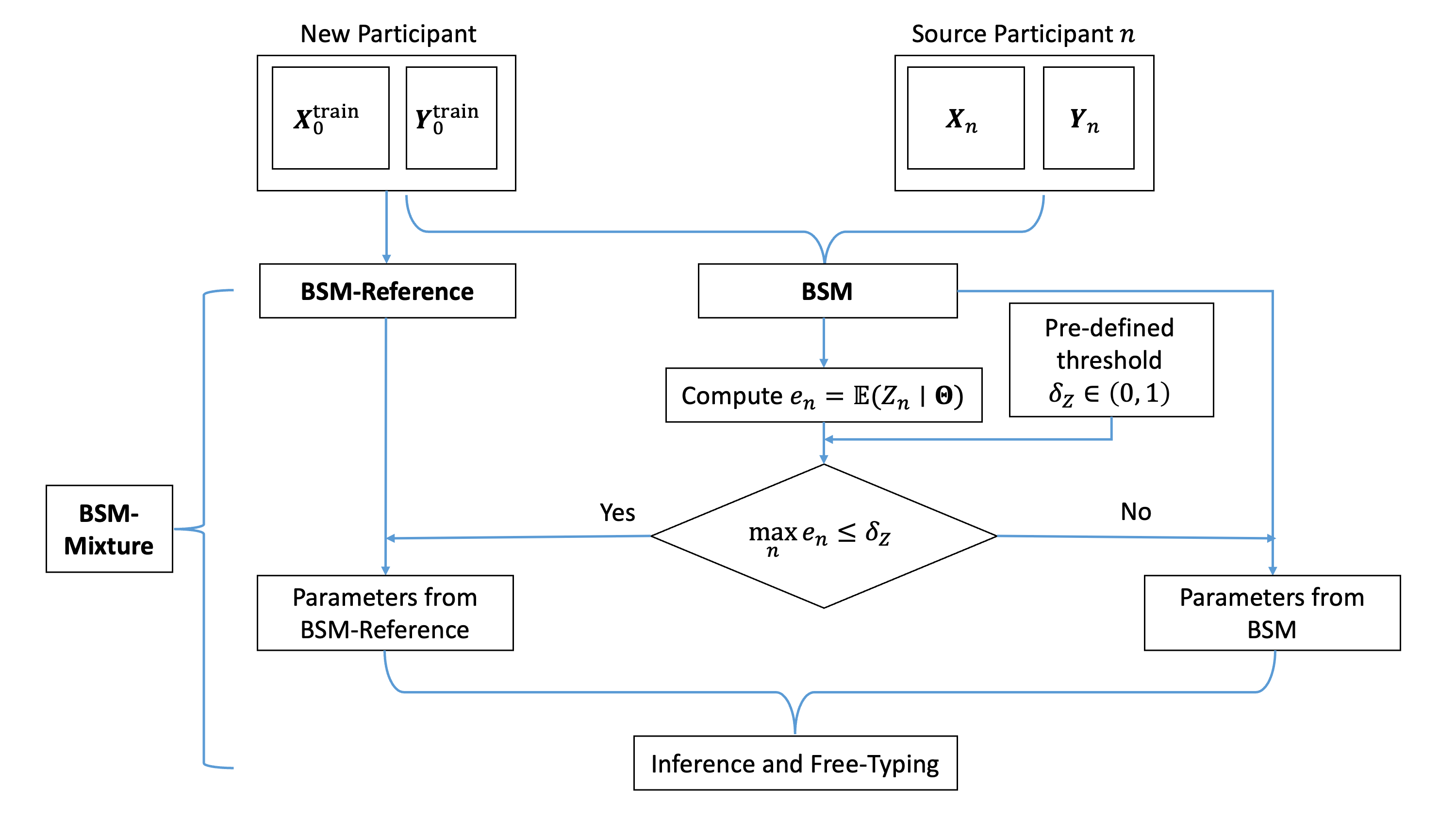
Figure 2: An illustration of the BSM-Mixture algorithm. First, we pre-defined a threshold $\delta_{Z}\in(0,1)$. Second, we fitted BSM model and obtained posterior samples of $\{Z_{n}\}$ to compute $\mathbb{E}(Z_{n}\mid\bm{\Theta})$. If none of the posterior expectations exceeded $\delta_{Z}$, we applied BSM-Reference, otherwise, we applied BSM model for prediction. Note that both BSM-Reference and BSM models can be fitted simultaneously, and it will not have extra computational burden to the total calibration effort.

3.3 Hybrid Model Selection Strategy: BSM-Mixture

Since our primary goal was to use small amount of training data from the new participant for calibration data, it might be challenging for our BSM model to identify source participants when no source participants were available for matching. In practice, we proposed the hybrid model selection strategy, namely BSM-Mixture, such that if no source participants were selected satisfying certain threshold, we simply used BSM-Reference for prediction. We defined the hybrid model selection strategy as follows: First, we pre-defined a threshold $\delta_{Z}\in(0,1)$. Second, we fitted BSM model and obtained the posterior samples of $\{Z_{n}\}$ to compute $\mathbb{E}(Z_{n}\mid\bm{\Theta})$. If none of $\mathbb{E}(Z_{n}\mid\bm{\Theta})$ exceeded $\delta_{Z}$, we applied BSM-Reference, otherwise, we applied BSM model for prediction. Note that BSM-Reference and BSM model could be fitted simultaneously, it did not add much computational burden to the total calibration effort. Figure 2 provides an illustration of the hybrid model selection strategy on BSM-Mixture.

3.4 Posterior Character-Level Prediction

One of the advantages of our method is to predict on testing data directly without refitting the data. Under the RCP design, the character-level prediction depends on selecting the correct row and column within each sequence. Let $\bm{W},\bm{Y}$, and $\bm{X}$ be existing stimulus-code indicators, stimulus-type indicators, and matrix-wise EEG signals, respectively. Let $\bm{W}_{0}^{*},\bm{Y}_{0}^{*},\bm{X}_{0}^{*}$, and $\bm{\Theta}_{0}$ be additional one sequence of stimulus-code indicators, stimulus-type indicators, matrix-wise EEG signals, and the parameter set, respectively, associated with the new participant. To simplify the notation, we assume that the new participant is spelling the same target character $\omega$. Based on the property described in Section 2.1, let $\bm{y}^{*}_{\omega}$ be the possible values of stimulus-type indicators given $\bm{W}_{0}^{*}$ and the target character $\omega$.

$$\operatorname{Pr}(\bm{Y}_{0}^{*}=\bm{y}^{*}_{\omega}\mid\bm{X}_{0}^{*},\bm{W}_{0}^{*},\bm{X},\bm{W},\bm{Y}) =\int\operatorname{Pr}(\bm{Y}_{0}^{*}=\bm{y}^{*}_{\omega}\mid\bm{\Theta}_{0};\bm{X}_{0}^{*},\bm{W}_{0}^{*})\operatorname{Pr}(\bm{\Theta}_{0}\mid\bm{X},\bm{W},\bm{Y})d\bm{\Theta}_{0},$$ (12)

$$\operatorname{Pr}(\bm{Y}_{0}^{*}=\bm{y}^{*}_{\omega}\mid\bm{\Theta}_{0};\bm{X}_{0}^{*},\bm{W}_{0}^{*}) \propto\underbrace{\operatorname{Pr}(\bm{X}_{0}^{*}\mid\bm{\Theta}_{0};\bm{W}_{0}^{*},\omega)}_{\text{Equation }\eqref{eq:matrix_normal_model}}\cdot\operatorname{Pr}(\omega\text{ is target}),$$

Here, $\operatorname{Pr}(\omega\text{ is target})=1/36$ is the predictive prior on each candidate character with non-informative priors under the RCP design. When we need multiple sequence replications to select the target character, we modify the above formula by multiplying the sequence-specific posterior conditional likelihood within each cluster.

4 Simulation Studies

We conducted extensive simulation studies to demonstrate the advantage of our proposed framework. We showed the results of the multi-channel simulation scenario in this section and moved the results of the single-channel scenario to the supplemental material.
Setup  We considered the scenario with $N=7$ and $K=3$. We designed three groups of parameters including two-dimensional pre-specified mean ERP functions and variance nuisance parameters. The shape and magnitude were based on real participants from the database (Thompson et al.,, 2014). The simulated EEG signals were generated with a response window of 35 time points per channel, i.e., $T_{0}=35$. For simulated data generated from group 0, we created a typical P300 pattern for the first channel where the target ERP function reached its positive peak around 10th time point post stimulus and reversed the sign for both ERP functions for the second channel; for simulated data generated from group 1, we created the same target ERP function as group 0 for the first channel and reduced the peak magnitude for the second channel; for simulated data generated from group 2, we reduced the peak magnitude for the first channel and created the same ERP functions as group 1 for the second channel. We considered an autoregressive temporal structure of order 1 (i.e., AR(1)), compound symmetry spatial structure, and channel-specific variances for background noises, where the true parameters for groups 0, 1, and 2 were $(\rho_{0}=0.7,\eta_{0}=0.6,\sigma_{0,1}=8.0,\sigma_{0,2}=8.0)$, $(\rho_{1}=0.7,\eta_{1}=0.4,\sigma_{1,1}=8.0,\sigma_{1,2}=6.0)$, and $(\rho_{2}=0.5,\eta_{2}=0.4,\sigma_{2,1}=2.0,\sigma_{2,2}=2.0)$, respectively. We still designed two cases for this scenario, a case without matched data among source participants (Case 1) and a case with matched data (Case 2). For Case 1, the group labels for source participants 1-6 were 1, 1, 1, 2, 2, and 2, respectively. For Case 2, the group labels for source participants 1-6 were 0, 0, 1, 1, 2, and 2, respectively. We performed 100 replications for each case. Within each replication, we assumed that each participant was spelling three characters “TTT” with ten sequence replications per character for training and generated additional testing data of the same size as the testing data of the single-channel scenario.

Settings and Diagnostics  All simulated datasets were fitted with equation (6). We also applied two covariance kernels $\kappa_{1}$ and $\kappa_{0}$ for target and non-target ERP functions, respectively. The two kernels were characterized by $\gamma$-exponential kernels with length-scale and gamma hyper-parameters as $(0.2,1.2)$ and $(0.3,1.2)$, respectively. The pre-specified threshold $\delta_{Z}$ was $0.5$. We ran the MCMC with three chains, with each chain containing 3000 burn-ins and 300 MCMC samples. The Gelman-Rubin statistics were evaluated.

Table 1: The means and standard deviations of testing sequence sizes to achieve a 95% testing accuracy given certain training sequence sizes for BSM-Mixture, BSM, MDWM, BSM-Reference, and swLDA across 100 replications. For Case 1, the testing sequence sizes of BSM-Mixture were smaller or close to MDWM and swLDA although the testing sequence sizes of BSM were consistently larger than those of BSM-Reference, suggesting that the strategy of BSM-Mixture favored BSM-Reference when no one was selected; For Case 2, the testing sequence sizes of BSM-Mixture were consistently smaller than MDWM and swLDA, and the strategy of BSM-Mixture favored BSM when at least one source participant was selected.

	Train	Test Sequence Size
	Seq Size	BSM-Mixture	BSM	MDWM	BSM-Reference	swLDA
Case 1	2	8.4, 1.7	9.8, 0.7	7.9, 1.6	8.2, 1.7	10.0, 0.3
	3	7.6, 1.8	9.6, 1.1	7.8, 1.6	7.6, 1.8	9.8, 0.6
	4	7.2, 1.7	9.3, 1.1	7.8, 1.4	7.1, 1.7	9.6, 0.9
Case 2	2	7.3, 1.6	7.3, 1.7	7.9, 1.6	8.2, 1.7	10.0, 0.3
	3	7.2, 1.8	7.2, 1.8	7.9, 1.6	7.6, 1.8	9.8, 0.6
	4	6.8, 1.7	6.8, 1.7	7.8, 1.5	7.1, 1.7	9.6, 0.9

Table 2: The mean and standard deviations of training sequence size to achieve a 95% testing accuracy given certain testing sequence sizes for BSM-Mixture, BSM, MDWM, BSM-Reference, and swLDA across 100 iterations. For Case 1, the training sequence sizes of BSM-Mixture were consistently smaller than MDWM and swLDA although BSM had larger training sequence sizes than BSM-Reference, suggesting that the strategy of BSM-Mixture favored BSM-Reference when no one was selected; For Case 2, the training sequence sizes of BSM-Mixture are consistently smaller than MDWM and swLDA, and the strategy of BSM-Mixture favored BSM when at least one source participant was selected.

	Test	Train Sequence Size
	Seq Size	BSM-Mixture	BSM	MDWM	BSM-Reference	swLDA
Case 1	5	8.0, 3.0	9.2, 1.7	9.0, 2.5	8.0, 3.1	9.7, 1.2
	6	6.3, 3.4	8.3, 2.2	7.5, 3.5	6.3, 3.5	9.2, 1.6
	7	4.9, 3.4	7.1, 2.9	5.2, 3.9	4.9, 3.5	8.7, 2.1
Case 2	5	7.5, 3.5	7.4, 3.5	8.9, 2.6	8.0, 3.1	9.7, 1.2
	6	5.7, 4.1	5.8, 4.1	7.5, 3.4	6.3, 3.5	9.2, 1.6
	7	3.8, 3.7	3.9, 3.7	5.3, 4.0	4.9, 3.5	8.7, 2.1

Criteria  We evaluated our method by matching and prediction. For matching, we reported the proportion that each source participant was matched to the new participant and produced the ERP function estimates with 95% credible bands with respect to the training sequence size. For prediction, we reported the character-level prediction accuracy of the testing data, using Bayesian signal matching with source participants’ data (BSM), Bayesian generative methods with the new participant’s data only (BSM-Reference), the hybrid model selection strategy (BSM-Mixture), an existing classification method with data borrowing using Riemannian Geometry (MWDM), and swLDA with new participant’s data only (swLDA). We did not include SMGP for comparison in the simulation studies because SMGP assumed that data were generated under sequences of stimuli, while our data generative mechanism was based on each stimulus. We did not include other conventional ML methods because we assume that the prediction accuracy of swLDA was representative of those types of methods.

Table 3: Upper Panel: A summary of means and standard deviations of $Z_{n}=1$ for Case 1 across 100 replications. Lower Panel: A summary of means and standard deviations of $Z_{n}=1$ for Case 2 across 100 replications. The results were produced by BSM. The numerical values were multiplied by 100 for convenience and were reported with respect to the training sequence replications. For Case 1, all the values quickly decreased below 10.0 with 3 training sequence replications; for Case 2, values associated with Participants 1-2 were above 0.75 across all training sequence replications and values associated with Participants 3-6 were below 10.0 within 4 sequence replications. The results indicated that our method correctly performed the participant selection.

Participant ID	Sequence Size
	1	2	3	4	5	6	7	8	9	10
1	31.7, 25.6	14.3, 18.5	8.2, 13.6	9.1, 14.8	8.7, 14.6	7.2, 13.7	7.9, 14.0	8.8, 15.4	8.2, 15.1	7.8, 13.2
2	28.5, 26.3	15.3, 19.8	9.8, 16.6	9.5, 17.0	9.8, 16.6	7.5, 15.4	8.1, 13.6	6.8, 12.5	8.8, 14.0	9.2, 14.9
3	32.8, 26.2	15.3, 19.3	9.2, 15.0	11.4, 17.2	8.9, 14.7	9, 15.7	11.1, 17.1	7.2, 13.7	6.5, 12.3	9.4, 15.8
4	1.3, 3.3	1.6, 4.5	1.1, 0.3	1.4, 3.3	0.9, 0.3	0.9, 0.3	1.3, 3.3	1.0, 0.3	1.0, 0.3	1.7, 4.6
5	2.3, 6.4	1.4, 3.3	1.7, 4.6	2.3, 6.4	1.0, 0.3	1.0, 0.3	1.0, 0.3	1.6, 4.6	2.0, 5.7	1.3, 3.2
6	1.0, 0.4	1.0, 0.3	1.7, 4.6	1.0, 0.3	1.7, 4.6	1.3, 3.3	1.3, 3.2	1.7, 4.6	1.3, 3.3	2.0, 5.6
Participant ID	Sequence Size
	1	2	3	4	5	6	7	8	9	10
1	75.9, 22.9	83.0, 20.0	89.0, 16.0	87.8, 17.9	92.3, 13.3	92.5, 14.1	92.2, 15.0	92.9, 13.2	93.3, 11.4	93.2, 13.4
2	76.5, 22.0	81.0, 21.4	87.9, 17.6	87.3, 18.7	92.6, 14.2	91.2, 16.5	92.2, 14.1	91.8, 14.8	91.6, 15.2	91.2, 14.1
3	15.5, 19.7	10.0, 14.5	12.4, 17.5	8.2, 15.1	6.6, 12.3	10.0, 15.4	6.9, 13.4	4.3, 10.9	6.8, 14.1	7.9, 14.1
4	12.1, 18.0	11.7, 15.4	12.1, 18.6	9.2, 16.5	9.1, 16.3	7.5, 13.1	9.0, 15.5	8.2, 14.3	7.8, 14.8	6.5, 12.3
5	1.7, 4.5	1.0, 0.3	1.0, 0.4	1.3, 3.3	1.0, 0.3	1.0, 0.3	1.6, 4.6	2.0, 5.6	1.3, 3.3	1.0, 0.3
6	1.4, 3.3	1.0, 0.3	1.3, 3.3	1.3, 3.2	1.0, 0.3	1.1, 0.3	1.0, 0.3	0.9, 0.3	1.0, 0.3	1.0, 0.4

Matching Results  The upper and lower panels of Table 3 show the means and standard deviations of $Z_{n}=1$ across 100 replications for cases without and with matched data, respectively, by BSM. The numerical values were multiplied by 100 for convenient reading and were reported with respect to the training sequence size of the new participant. For Case 1, all the values quickly dropped below 10.0 with 3 training sequence replications; for Case 2, values associated with Participants 1-2 were above 75.0 across all the training sequences and values associated with Participants 3-6 quickly dropped below 10.0 within 4 sequence replications. The results indicated that our method correctly performed the participant selection.

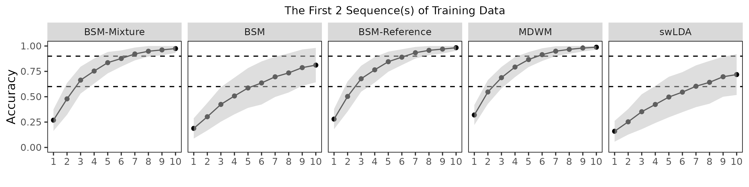
Figure 3: Means and standard errors of testing prediction accuracy by BSM-Mixture, BSM, BSM-Reference, MDWM, and swLDA of Case 1. The upper, middle, and lower panels show prediction accuracy with the first 2, 3, and 4 training sequence replications, respectively.

Figure 4: Means and standard errors of testing prediction accuracy by BSM-Mixture, BSM, BSM-Reference, MDWM, and swLDA of Case 2. The upper, middle, and lower panels show prediction accuracy with the first 2, 3, and 4 training sequence replications, respectively.

Prediction Results  Figure 3 shows the means and standard errors of testing prediction accuracy of Case 1 (No Matched) by BSM-Mixture, BSM, BSM-Reference, MDWM, and swLDA. The testing prediction accuracy is further stratified by training the first 2, 3, and 4 sequences of the new participant. Within the same row, BSM-Mixture and BSM-Reference had similar performances to MDWM. The poor performance of BSM was due to the uncertainty among participant selection in presence of no source participant and small training sample size. Therefore, the hybrid model selection strategy solved this issue. Within the same column, all four methods themselves performed better as training data of the new participant increased.

Figure 4 shows the means and standard errors of testing prediction accuracy of Case 2 (Matched) by BSM-Mixture, BSM, BSM-Reference, MWDM, and swLDA. The testing prediction accuracy is also stratified by training the first 2, 3, and 4 training sequences of the new participant. Within the same row, BSM-Mixture performed the best, followed by MDWM, suggesting that our method successfully identified the matched participants and leveraged their information correctly. Within the same column, all four methods themselves performed better as training data of the new participant increased.

5 Analysis of BCI data from Real Participants

We examined the performance of our BSM framework on real-participant data, where the real data were originally collected from the XXX Lab. A total of 41 participants were recruited to accomplish the experiment, but we restricted our study population to 9 participants with brain damages or neuro-degenerative diseases. Each participant completed both a calibration (training) session (TRN) and several free-typing sessions (FRT). For the calibration session, each participant was asked to copy a 19-character phrase “THE_QUICK_BROWN_FOX” including three spaces with 15 sequences, while wearing an EEG cap with 16 channels and sitting close to a monitor with a virtual keyboard. Details can be found Thompson et al., (2014).

The steps of real data analysis were as follows: First, we performed a series of data pre-processing techniques on the raw EEG signals of each participant. Next, we identified a proper source participant pool based on testing swLDA accuracy. We trained swLDA and SMGP using the calibration data from the new participant only as two reference methods and trained BSM-Mixture and MDWM including source data from source participants as two mixture models. We did not include other conventional ML methods because they did not have the borrowing version and we argued that swLDA could serve as the performance baseline for other ML methods. We demonstrated the result of a particular participant K151, a senior male diagnosed with amyotrophic lateral sclerosis (ALS) and showed the results of the remaining cohort in the supplementary materials.

5.1 Data Pre-processing Procedure and Model Fitting

We applied the band-pass filter between 0.5 Hz and 6 Hz and down-sampled the EEG signals with a decimation factor of 8. Next, we extracted a fixed response window of approximately 800 ms after each event such that the resulting EEG matrix contained 15 sequence segments, and each sequence contained 12 extracted event-related EEG signal segments. The resulting event-related EEG signal segment had around 800 ms, i.e., 25 sampling points per channel. Since the SNR of EEG signals is typically low, we further applied the xDAWN algorithm to enhance the evoked potentials (Rivet et al.,, 2009). The xDAWN method was an unsupervised algorithm that decomposed the raw EEG signals into relevant P300 ERPs and background noises and aimed to find a robust spatial filter that projected raw EEG signal segments onto the estimated P300 subspace by directly modeling noise in the objective function. We used all 16 channels as the signal input and selected the first two major components. We will denote raw EEG signal inputs and ERP functions after the xDAWN algorithm as transformed EEG signals and transformed ERP functions, respectively.

To emphasize the calibration-less point, we used a small portion of K151’s training set and abundant training set from source participants for calibration. We identified 23 participants whose prediction accuracy of swLDA on FRT files exceeded 50% and used them as the source participant pool: For each source participant, we included the first ten sequence replications of the first five characters: “THE_Q” (17.5% of the entire calibration data), and the testing prediction accuracy was obtained with all FRT files (up to three sessions per participant). For K151, we included the first five sequence replications of the same five characters (8.8% of the entire calibration data). Therefore, the resulting EEG feature matrices for the new participant and source participants had sizes of (180, 2, 25) and (360, 2, 25), respectively. Here, 180, 360, 2, and 25 were the number of stimuli for new participant, the number of stimuli for source participants, the number of transformed ERP components and the length of EEG response window, respectively.

The datasets were fitted with the equation (6). We applied two covariance kernels $\kappa_{1}$ and $\kappa_{0}$ for target and non-target ERP functions, respectively. Two kernels were characterized by $\gamma$-exponential kernels with length-scale and gamma hyper-parameters as $(0.2,1.2)$ and $(0.3,1.2)$, respectively. The pre-specified threshold $\delta_{Z}$ was 0.02. We ran the MCMC with three chains, with each chain containing 3000 burn-ins and 300 MCMC samples. The Gelman-Rubin statistics were computed to evaluate the convergence status of each model. We examined two perspectives on model fitting: matching and prediction. For matching, we reported the selection indicator $Z_{n}$. We also produced the transformed EEG signal function estimates by BSM and compared them to the results by BSM-Reference. For prediction, we reported the prediction accuracy on FRT files by BSM-Mixture, MDWM, swLDA, and SMGP up to five testing sequences. We only reported BSM-Mixture to utilize both advantages of BSM and BSM-Reference. We also included the Split-and-Merge Gaussian Process (SMGP) method (Ma et al.,, 2022) as another method for comparison. The SMGP method primarily focused on detecting the spatial-temporal discrepancies on brain activity between target and non-target ERP functions under the sequence-based analysis framework, which was different from our stimulus-based analysis framework.

5.2 Matching and Prediction Results

Figure 5 shows the inference results of K151. The first columns show the mean estimates and their 95% credible bands of the first two transformed ERP functions by BSM-Mixture. Only target ERP information was borrowed. The right two columns show the spatial pattern and spatial filter of the new participant’s partial training data by xDAWN. The average value of $\{Z_{n}\}$ among source participants was around 1.0%. Given the general low signal-to-noise ratio property, it indicated that the borrowing results were not dominated by certain source participant.

For Component 1, we observed a sinusoidal pattern such that the transformed ERP response achieved a minor positive peak around 50 ms post stimulus and a major negative peak around 200 ms post stimulus. The signal achieved its second positive peak around 350 ms post stimulus and gradually decreased to zero. Spatial pattern and filter plot indicated that the major negative peak was primarily attributed to parietal-occipital and occipital regions (channels PO7, PO8, and Oz). For Component 2, we observed a Mexican-hat pattern with a double-camel-hump feature. The transformed target ERP response achieved its first negative peak around 100 ms post stimulus and its two positive peaks around 250 ms and 450 ms post stimulus before it gradually decreased to zero. Spatial pattern and filter plot indicated that such double-positive peak was primarily attributed to central and parietal regions.

Figure 5: The first column shows the mean estimates with 95% credible bands of the first two transformed ERP functions by BSM-Mixture. Only target ERP information was borrowed. The right two columns show the spatial patterns and spatial filters of the new participant’s partial training data by xDAWN.

Table 4: Prediction accuracy (percentage) of all FRT files with up to five testing sequences by BSM-Mixture, MDWM, swLDA, and SMGP with five training sequences.

Testing	Mixture Methods		Reference Methods
Sequence Size	BSM-Mixture	MDWM	swLDA	SMGP
1	54.1%	47.3%	37.8%	16.2%
2	77.0%	71.6%	50.0%	23.0%
3	81.1%	75.7%	67.6%	40.5%
4	89.2%	81.9%	75.7%	39.2%
5	90.5%	90.5%	81.1%	51.4%

Table 4 shows the total prediction accuracy of all FRT files with respect to the testing sequences up to five by BSM-Mixture, MDWM, swLDA, and SMGP with five training sequences for K151. Overall, BSM-Mixture performed better than two reference methods. BSM-Mixture achieved 80% accuracy within 3 testing sequences, which was slightly faster than the existing method MDWM. Unfortunately, the SMGP method performed poorly in this case due to different assumptions in the analysis framework. The SMGP method treated one sequence of EEG data as an analysis unit, while our BSM framework treated one stimulus of EEG data as an analysis unit. Therefore, under the RCP design, the sample size for SMGP was 1/12 of that for BSM-Mixture, which led to inaccurate estimation of P300 response functions and poor prediction on FRT files.

In general, the advantage of BSM-Mixture was reflected in later testing sequences when participants were more likely to get distracted and have a higher heterogeneity level of EEG signals over time. Certain temporal intervals might become less separable and the attenuated amplitude estimates on these potentially confusing regions by BSM-Mixture actually reduced the negative effect of growing signal heterogeneity on prediction accuracy. For K151, temporal regions such as [500 ms, 800 ms] of Component 1, the double peaks of Component 2 by BSM-Mixture were attenuated than those by BSM-Reference. However, that the initial 100 ms and intervals around 350 ms of Component 1 became even more separable by BSM-Mixture might indicated that those intervals were robust over time and essential to maintain high prediction accuracy during FRT tasks.

Figure 6: A Spaghetti plot of character-level testing accuracy by BSM-Mixture, MDWM,, swLDA, and SMGP for 9 participants with at most 5 testing sequences and 5 training sequences. Means of each method were shown in red.

6 Discussion

In this article, we proposed a hierarchical Bayesian Signal Matching (BSM) framework to build a participant-semi-dependent, calibration-less framework with applications to P300 ERP-based Brain-Computer Interfaces. The BSM framework reduced the sample size for calibration of the new participant by borrowing data from pre-existing source participants’ pool at the participant level. The BSM framework specified the joint distribution of stimulus-related EEG signal inputs via a Bayesian hierarchical mixture model. Unlike conventional clustering approaches, our method specified the baseline cluster associated with the new participant and conducted pairwise comparisons between each source participant and the new participant by the criterion of log-likelihood. In this way, our method avoided the cluster label switching issue and could pre-compute model parameters from source participants to speed up the calibration in practice. In addition, since our method intrinsically borrowed the information from source participants via the binary selection indicators, we could use parameters from the baseline cluster to test directly without refitting the model with the augmented data. Finally, our hierarchical framework was base-model-free, such that it could be extended to any other classifiers with clear likelihood functions. We demonstrated the advantages of our method using extensive single- and multi-channel simulation studies and focused on the real data analysis among the cohort with brain injuries and neuro-degenerative diseases.

In the real data analysis, we found that first transformed ERP response was associated with the effect of visual cortex (higher positive values within parietal-occipital and occipital regions, while close to zero elsewhere) and that the second transformed ERP response was associated with the typical P300 responses (higher positive values within central and parietal regions). The resulting pattern with double-camel humps might be due to the effect of latency jitter (Guy et al.,, 2021) or simply the superimposed effect of various signal contributions from central and parietal electrodes by xDAWN. The cross-participant results also suggested that major negative peaks before 200 ms and positive peaks around 350 ms post stimulus were preserved in the first two transformed ERP responses. The above scientific findings were consistent with the finding from our previous study Ma et al., (2022) that the performance of the P300 speller greatly depended on the effect of the visual cortex, in addition to electrodes located in central and parietal regions.

In addition, compared to the simulation studies, the borrowing results of the real data analysis did not depend on certain source participants. Several reasons accounted for the results: First, the data generation mechanism of our method assumed that each observed EEG signal input was generated independently across stimuli, while the real data were extracted with overlapping EEG components between adjacent stimuli, and the overlapping temporal feature still existed after applying the xDAWN filter. It was a potential model mis-specification to apply our method to the real data, which might make it difficult to find a very good match on the participant level. Second, our similarity criterion was based on calculating the log-likelihood of the target transformed ERP functions using the generative base classifier, which might be more sensitive to noise than discriminant classifiers. In simulation studies, the noises were clearly defined and well controlled, while in the real data analysis, the noises might not be normally distributed, and the heterogeneity level of data increased not only across participants but also within the same participant over time, and the growing variability of data tended to diminish the magnitudes of transformed ERPs. Fortunately, since BSM modeled the selection indicator in a soft-threshold manner, it had a flavor of Bayesian averaging that generally attenuated the magnitudes of peaks. Such diminishing differences between target and non-target transformed ERP function estimates actually contributed to the prediction accuracy by suppressing the separability of temporal intervals with higher uncertainty.

For cross-participant analysis, the transformed ERP function estimates of BSM were consistently attenuated compared to BSM-Reference, and the patterns of first two components were similar across nine participants. Figure 6 demonstrates the prediction accuracy of our target population cohort by BSM-Mixture, MDWM, swLDA, and SMGP. BSM-Mixture has similar prediction accuracy to MDWM, and they performed better than two reference methods. The improvements in BSM-Mixture and MDWM confirmed that people with brain injuries or neuro-degenerative diseases could definitely benefit from data borrowing, especially because they were the population who needed this type of assistance the most for daily communication.

There were some limitations to our study. First, the generative base classifier we used was still sensitive to background noise compared to conventional discriminant classifiers. It might overly extract information from source participants to overfit the model. Second, the generative classifier might require careful tuning of hyperparameters such as the kernel hyperparameter selection of Gaussian process priors. The current strategy is to determine the values with heuristics, which might potentially affect the inference results and the prediction accuracy. Finally, although selection at the participant level was an intuitive idea, the characteristic of heterogeneity over time within the same participant suggested that we should have secondary sequence-level binary selection indicators. However, a side analysis of using sequence-level BSM-Mixture surprisingly performed worse than the one using participant-level selection indicators. It might be due to the fact that such refined selection indicators paired with generative base classifiers might overfit the training data and therefore had less power to generalize to the FRT data over time. Nevertheless, our main contribution was to demonstrate the advantages of the proposed hierarchical signal-matching framework, and the current framework could be expanded and improved in alternative ways.

For future work, first, we would replace the generative base classifier with other robust discriminant classifiers, e.g., Riemannian geometry. The entire framework would remain unchanged except that we would specify the likelihood function by introducing Riemannian Gaussian distributions (Zanini et al.,, 2016), (Said et al.,, 2017). Even if we followed the generative pathway for classifiers, despite the poor performance of the original SMGP, it could be further improved by a slight modification. Since the original SMGP method focused on inferring on spatial-temporal brain activity under the P300 ERP-BCI setting rather than prediction, it usually required a large sample size for model fitting. Therefore, if we continued using the current generative Bayesian classifier, we would adopt the idea of split-and-merge to explicitly control the discrepancies between target and non-target (transformed) EEG signals, i.e., the temporal interval close to 800 ms on the stimulus level. Finally, we would incorporate our framework into calibration-free methods (Verhoeven et al.,, 2017). In addition to borrowing the training data from source participants and testing separately, we would directly start testing on the new participant and dynamically update the parameters of the baseline group as the data arrive, known as calibration-free methods.

References

- Adair et al., (2017) Adair, J., Brownlee, A., Daolio, F., and Ochoa, G. (2017). Evolving training sets for improved transfer learning in brain computer interfaces. In International Workshop on Machine Learning, Optimization, and Big Data, pages 186–197. Springer.
- An et al., (2020) An, X., Zhou, X., Zhong, W., Liu, S., Li, X., and Ming, D. (2020). Weighted subject-semi-independent erp-based brain-computer interface. In 2020 42nd Annual International Conference of the IEEE Engineering in Medicine & Biology Society (EMBC), pages 2969–2972. IEEE.
- Barachant et al., (2011) Barachant, A., Bonnet, S., Congedo, M., and Jutten, C. (2011). Multiclass brain–computer interface classification by riemannian geometry. IEEE Transactions on Biomedical Engineering, 59(4):920–928.
- Barachant and Congedo, (2014) Barachant, A. and Congedo, M. (2014). A plug&play p300 bci using information geometry. arXiv preprint arXiv:1409.0107.
- Bozinovski and Fulgosi, (1976) Bozinovski, S. and Fulgosi, A. (1976). The influence of pattern similarity and transfer learning upon training of a base perceptron b2. In Proceedings of Symposium Informatica, pages 3–121.
- Cecotti and Graser, (2010) Cecotti, H. and Graser, A. (2010). Convolutional neural networks for p300 detection with application to brain-computer interfaces. IEEE transactions on pattern analysis and machine intelligence, 33(3):433–445.
- Congedo et al., (2013) Congedo, M., Barachant, A., and Andreev, A. (2013). A new generation of brain-computer interface based on riemannian geometry. arXiv preprint arXiv:1310.8115.
- Dawid, (1981) Dawid, A. P. (1981). Some Matrix-variate Distribution Theory: Notational Considerations and a Bayesian Application. Biometrika, 68(1):265–274.
- Dixon and Crepey, (2018) Dixon, M. and Crepey, S. (2018). Multivariate gaussian process regression for portfolio risk modeling: Application to cva. Department of Applied Mathematics, Illinois Institute of Technology, 2018.
- Donchin et al., (2000) Donchin, E., Spencer, K. M., and Wijesinghe, R. (2000). The Mental Prosthesis: Assessing the Speed of a P300-based Brain-computer Interface. IEEE Transactions on Rehabilitation Engineering, 8(2):174–179.
- Farwell and Donchin, (1988) Farwell, L. A. and Donchin, E. (1988). Talking off the top of your head: toward a mental prosthesis utilizing event-related brain potentials. Electroencephalography and clinical Neurophysiology, 70(6):510–523.
- Gelman and Rubin, (1992) Gelman, A. and Rubin, D. B. (1992). Inference from Iterative Simulation using Multiple Sequences. Statistical Science, 7(4):457–472.
- Guy et al., (2021) Guy, M. W., Conte, S., Bursalıoğlu, A., and Richards, J. E. (2021). Peak selection and latency jitter correction in developmental event-related potentials. Developmental psychobiology, 63(7):e22193.
- Johnson and Krusienski, (2009) Johnson, G. D. and Krusienski, D. J. (2009). Ensemble swlda classifiers for the p300 speller. In International Conference on Human-Computer Interaction, pages 551–557. Springer.
- Kaper et al., (2004) Kaper, M., Meinicke, P., Grossekathoefer, U., Lingner, T., and Ritter, H. (2004). BCI Competition 2003-data Set IIb: Support Vector Machines for the P300 Speller Paradigm. IEEE Transactions on Biomedical Engineering, 51(6):1073–1076.
- Khazem et al., (2021) Khazem, S., Chevallier, S., Barthélemy, Q., Haroun, K., and Noûs, C. (2021). Minimizing subject-dependent calibration for bci with riemannian transfer learning. In 2021 10th International IEEE/EMBS Conference on Neural Engineering (NER), pages 523–526. IEEE.
- Krusienski et al., (2008) Krusienski, D. J., Sellers, E. W., McFarland, D. J., Vaughan, T. M., and Wolpaw, J. R. (2008). Toward Enhanced P300 Speller Performance. Journal of Neuroscience Methods, 167(1):15–21.
- Lenzerini, (2002) Lenzerini, M. (2002). Data integration: A theoretical perspective. In Proceedings of the twenty-first ACM SIGMOD-SIGACT-SIGART symposium on Principles of database systems, pages 233–246.
- Li et al., (2020) Li, F., Xia, Y., Wang, F., Zhang, D., Li, X., and He, F. (2020). Transfer learning algorithm of p300-eeg signal based on xdawn spatial filter and riemannian geometry classifier. Applied Sciences, 10(5):1804.
- Ma et al., (2022) Ma, T., Li, Y., Huggins, J. E., Zhu, J., and Kang, J. (2022). Bayesian inferences on neural activity in eeg-based brain-computer interface. Journal of the American Statistical Association, 117(539):1122–1133.
- Niedermeyer and da Silva, (2005) Niedermeyer, E. and da Silva, F. L. (2005). Electroencephalography: basic principles, clinical applications, and related fields. Lippincott Williams & Wilkins.
- Onishi, (2020) Onishi, A. (2020). Convolutional neural network transfer learning applied to the affective auditory p300-based bci. Journal of Robotics and Mechatronics, 32(4):731–737.
- Onishi and Natsume, (2014) Onishi, A. and Natsume, K. (2014). Overlapped partitioning for ensemble classifiers of p300-based brain-computer interfaces. PloS one, 9(4):e93045.
- Rakotomamonjy and Guigue, (2008) Rakotomamonjy, A. and Guigue, V. (2008). Bci competition iii: dataset ii-ensemble of svms for bci p300 speller. IEEE transactions on biomedical engineering, 55(3):1147–1154.
- Rivet et al., (2009) Rivet, B., Souloumiac, A., Attina, V., and Gibert, G. (2009). xdawn algorithm to enhance evoked potentials: application to brain–computer interface. IEEE Transactions on Biomedical Engineering, 56(8):2035–2043.
- Rodrigues et al., (2018) Rodrigues, P. L. C., Jutten, C., and Congedo, M. (2018). Riemannian procrustes analysis: transfer learning for brain–computer interfaces. IEEE Transactions on Biomedical Engineering, 66(8):2390–2401.
- Said et al., (2017) Said, S., Bombrun, L., Berthoumieu, Y., and Manton, J. H. (2017). Riemannian gaussian distributions on the space of symmetric positive definite matrices. IEEE Transactions on Information Theory, 63(4):2153–2170.
- Thompson et al., (2014) Thompson, D. E., Gruis, K. L., and Huggins, J. E. (2014). A Plug-and-play Brain-computer Interface to Operate Commercial Assistive Technology. Disability and Rehabilitation: Assistive Technology, 9(2):144–150.
- Verhoeven et al., (2017) Verhoeven, T., Hübner, D., Tangermann, M., Müller, K.-R., Dambre, J., and Kindermans, P.-J. (2017). Improving zero-training brain-computer interfaces by mixing model estimators. Journal of neural engineering, 14(3):036021.
- Völker et al., (2018) Völker, M., Schirrmeister, R. T., Fiederer, L. D., Burgard, W., and Ball, T. (2018). Deep transfer learning for error decoding from non-invasive eeg. In 2018 6th International Conference on Brain-Computer Interface (BCI), pages 1–6. IEEE.
- Wu et al., (2020) Wu, D., Xu, Y., and Lu, B.-L. (2020). Transfer learning for eeg-based brain–computer interfaces: A review of progress made since 2016. IEEE Transactions on Cognitive and Developmental Systems, 14(1):4–19.
- Xu et al., (2015) Xu, M., Liu, J., Chen, L., Qi, H., He, F., Zhou, P., Cheng, X., Wan, B., and Ming, D. (2015). Inter-subject information contributes to the erp classification in the p300 speller. In 2015 7th International IEEE/EMBS Conference on Neural Engineering (NER), pages 206–209. IEEE.
- Xu et al., (2016) Xu, M., Liu, J., Chen, L., Qi, H., He, F., Zhou, P., Wan, B., and Ming, D. (2016). Incorporation of inter-subject information to improve the accuracy of subject-specific p300 classifiers. International journal of neural systems, 26(03):1650010.
- Xu et al., (2004) Xu, N., Gao, X., Hong, B., Miao, X., Gao, S., and Yang, F. (2004). Bci competition 2003-data set iib: enhancing p300 wave detection using ica-based subspace projections for bci applications. IEEE transactions on biomedical engineering, 51(6):1067–1072.
- Zanini et al., (2016) Zanini, P., Congedo, M., Jutten, C., Said, S., and Berthoumieu, Y. (2016). Parameters estimate of riemannian gaussian distribution in the manifold of covariance matrices. In 2016 IEEE Sensor Array and Multichannel Signal Processing Workshop (SAM), pages 1–5. IEEE.
- Zhang et al., (2021) Zhang, L., Banerjee, S., and Finley, A. O. (2021). High-dimensional multivariate geostatistics: A bayesian matrix-normal approach. Environmetrics, 32(4):e2675.