Accelerated construction of projection-based reduced-order models via incremental approaches

Abstract

We present an accelerated greedy strategy for training of projection-based reduced-order models for parametric steady and unsteady partial differential equations. Our approach exploits hierarchical approximate proper orthogonal decomposition to speed up the construction of the empirical test space for least-square Petrov-Galerkin formulations, a progressive construction of the empirical quadrature rule based on a warm start of the non-negative least-square algorithm, and a two-fidelity sampling strategy to reduce the number of expensive greedy iterations. We illustrate the performance of our method for two test cases: a two-dimensional compressible inviscid flow past a LS89 blade at moderate Mach number, and a three-dimensional nonlinear mechanics problem to predict the long-time structural response of the standard section of a nuclear containment building under external loading.

Eki Agouzal^1,2, Tommaso Taddei²

¹ EDF Lab Paris-Saclay, 7 Boulevard Gaspard Monge, 91120, Palaiseau, France.
eki.agouzal@edf.fr
² Univ. Bordeaux, CNRS, Bordeaux INP, IMB, UMR 5251, F-33400 Talence, France.
Inria Bordeaux Sud-Ouest, Team MEMPHIS, 33400 Talence, France. eki.agouzal@inria.fr,tommaso.taddei@inria.fr

Keywords: model order reduction; greedy methods.

1 Introduction

In the past few decades, several studies have shown the potential of model order reduction (MOR) techniques to speed up the solution to many-query and real-time problems, and ultimately enable the use of physics-based three-dimensional models for design and optimization, uncertainty quantification, real-time control and monitoring tasks. The distinctive feature of MOR methods is the offline/online computational decomposition: during the offline stage, high-fidelity (HF) simulations are employed to generate an empirical reduced-order approximation of the solution field and a parametric reduced-order model (ROM); during the online stage, the ROM is solved to estimate the solution field and relevant quantities of interest for several parameter values. Projection-based ROMs (PROMs) rely on the projection of the equations onto a suitable low-dimensional test space. Successful MOR techniques should hence achieve significant online speedups at acceptable offline training costs. This work addresses the reduction of offline training costs of PROMs for parametric steady and unsteady partial differential equations (PDEs).

We denote by $\mu$ the vector of $p$ model parameters in the compact parameter region $\mathcal{P}\subset\mathbb{R}^{p}$; given the domain $\Omega\subset\mathbb{R}^{d}$ ($d=2$ or $d=3$), we introduce the Hilbert spaces $(\mathcal{X},\|\cdot\|)$ and $(\mathcal{Y},{\left|\kern-1.07639pt\left|\kern-1.07639pt\left|\cdot\right|\kern-1.07639pt\right|\kern-1.07639pt\right|})$ defined over $\Omega$. Then, we consider problems of the form

$${\rm find}\;u_{\mu}\in\mathcal{X}\;:\;\mathfrak{R}_{\mu}(u_{\mu},v)=0,\quad\forall\;v\in\mathcal{Y},\;\;\mu\in\mathcal{P},$$ (1)

where $\mathfrak{R}:\mathcal{X}\times\mathcal{Y}\times\mathcal{P}\to\mathbb{R}$ is the parametric residual associated with the PDE of interest. We here focus on linear approximations, that is we consider reduced-order approximations of the form

$$\widehat{u}_{\mu}=Z\widehat{\alpha}_{\mu},$$ (2)

where $Z:\mathbb{R}^{n}\to\mathcal{X}$ is a linear operator, and $n$ is much smaller than the size of the HF model; $\widehat{\alpha}:\mathcal{P}\to\mathbb{R}^{n}$ is the vector of generalized coordinates. As discussed in section 2, we here exploit the least-square Petrov-Galerkin (LSPG, [11]) ROM formulation proposed in [32]: the approach relies on the definition of a low-dimensional empirical test space $\widehat{\mathcal{Y}}\subset\mathcal{Y}$; furthermore, it relies on the approximation of the HF residual $\mathfrak{R}$ through hyper-reduction [29] to enable fast online calculations of the solution to the ROM. In more detail, we consider an empirical quadrature (EQ) procedure [18, 39] for hyper-reduction: EQ methods recast the problem of finding a sparse quadrature rule to approximate $\mathfrak{R}$ as a sparse representation problem and then resort to optimization algorithms to find an approximate solution. Following [18], we resort to the non-negative least-square (NNLS) method to find the quadrature rule.

In section 3, we also consider the application to unsteady problems: to ease the presentation, we consider one-step time discretizations based on the time grid $\{t^{(k)}\}_{k=0}^{K}$. Given $\mu\in\mathcal{P}$, we seek the sequence $\mathbb{u}_{\mu}=\{{u}_{\mu}^{(k)}\}_{k=0}^{K}$ such that

$$\left\{\begin{array}[]{ll}\displaystyle{\mathfrak{R}_{\mu}^{(k)}(u_{\mu}^{(k)},u_{\mu}^{(k-1)},v)=0}&\forall\,v\in\mathcal{Y};\\[8.53581pt] u_{\mu}^{(0)}=\bar{u}_{\mu}^{(0)};&\\[8.53581pt] \end{array}\right.$$ (3)

for all $\mu\in\mathcal{P}$. As for the steady-state case, we consider linear ansatzs of the form $\widehat{u}_{\mu}^{(k)}=Z\widehat{\alpha}_{\mu}^{(k)}$, where $Z:\mathbb{R}^{n}\to\mathcal{X}$ is a linear time- and parameter-independent operator, and $\widehat{\alpha}^{(0)},\ldots,\widehat{\alpha}^{(K)}:\mathcal{P}\to\mathbb{R}^{n}$ are obtained by projecting the equations (3) onto a low-dimensional test space. To speed up online costs, we also replace the HF residual in (3) with a rapidly-computable surrogate through the same hyper-reduction technique considered for steady-state problems.

Following the seminal work by Veroy [34], numerous authors have resorted to greedy methods to adaptively sample the parameter space, with the ultimate aim of reducing the number of HF simulations performed during the training phase. Algorithm 1 summarizes the general methodology. First, we initialize the reduced-order basis (ROB) $Z$ and the ROM based on a priori sampling of the parameter space; second, we repeatedly solve the ROM and we estimate the error over a range of parameters $\mathcal{P}_{\rm train}\subset\mathcal{P}$; third, we compute the HF solution for the parameter that maximizes the error indicator; fourth, if the error is above a certain threshold, we update the ROB $Z$ and the ROM, and we iterate; otherwise, we terminate. Note that the algorithm depends on an a posteriori error indicator $\Delta$: if $\Delta$ is a rigorous a posteriori error estimator, we might apply the termination criterion directly to the error indicator (and hence save one HF solve). The methodology has been extended to unsteady problems in [21]: the method in [21] combines a greedy search driven by an a posteriori error indicator with proper orthogonal decomposition (POD, [30, 35]) to compress the temporal trajectory.

Algorithm 1 : abstract weak greedy algorithm.

1:Choose $\mathcal{P}_{\star}=\{\mu^{\star,i}\}_{i=1}^{n_{0}}$ and compute the HF solutions $\mathcal{S}_{\star}=\{{u}_{\mu}^{\rm hf}:\mu\in\mathcal{P}_{\star}\}$.

2:for $n=n_{0}+1,\ldots,n_{\rm max}$ do

3:     Update the ROB ${Z}$ and the ROM.

4:     Compute the estimate $\widehat{u}_{\mu}^{\rm hf}$ and evaluate the error indicator $\Delta_{\mu}$ for all $\mu\in\mathcal{P}_{\rm train}$.

5:     Compute $u_{\mu^{\star,n}}^{\rm hf}$ for $\mu^{\star,n}={\rm arg}\max_{\mu\in\mathcal{P}_{\rm train}}\Delta_{\mu}$; update $\mathcal{P}_{\star}$ and $\mathcal{S}_{\star}$.

6:     if $\|{u}_{\mu^{\star,n}}^{\rm hf}-\widehat{u}_{\mu^{\star,n}}\|<{\texttt{tol}}\|{u}_{\mu^{\star,n}}^{\rm hf}\|$ then

7:         Update the ROB ${Z}$ and the ROM.

8:         break

9:     end if

10:end for

As observed by several authors, greedy methods enable effective sampling of the parameter space [14]; however, they suffer from several limitations that might ultimately limit their effectiveness compared to standard a priori sampling. First, Algorithm 1 is inherently sequential and cannot hence benefit from parallel architectures. Second, Algorithm 1 requires the solution to the ROM and the evaluation of the error indicator for several parameter values at each iteration of the offline stage; similarly, it requires the update of the ROM — i.e., the trial and test bases, the reduced quadrature, and possibly the data structures employed to evaluate the error indicator. These observations motivate the development of more effective training strategies for MOR.

We propose an acceleration strategy for Algorithm 1 based on three ingredients: (i) a hierarchical construction of the empirical test space for LSPG ROMs based on the hierarchical approximate POD (HAPOD, [23]); (ii) a progressive construction of the empirical quadrature rule based on a warm start of the NNLS algorithm; (iii) a two-fidelity sampling strategy that is based on the application of the strong-greedy algorithm (see, e.g., [28, section 7.3]) to a dataset of coarse simulations. Re (iii), sampling based on coarse simulations is employed to initialize Algorithm 1 (cf. Line 1) and ultimately reduce the number of expensive greedy iterations. We illustrate the performance of our method for two test cases: a two-dimensional compressible inviscid flow past a LS89 blade at moderate Mach number, and a three-dimensional nonlinear mechanics problem to predict the long-time structural response of the standard section of a nuclear containment building (NCB) under external loading.

Our method shares several features with previously-developed techniques. Incremental POD techniques have been extensively applied to avoid the storage of the full snapshot set for unsteady simulations (see, e.g., [23] and the references therein): here, we adapt the incremental approach described in [23] to the construction of the test space for LSPG formulations. Chapman [13] extensively discussed the parallelization of the NNLS algorithm for MOR applications: we envision that our method can be easily combined with the method in [13] to further reduce the training costs. Several authors have also devised strategies to speed up the greedy search through the vehicle of a surrogate error model [19, 27]; our multi-fidelity strategy extends the work by Barral [6] to unsteady problems and to a more challenging — from the perspective of the HF solver — compressible flow test. We remark that our approach is similar in scope to the work by Benaceur [8] that devised a progressive empirical interpolation method (EIM, [7]) for hyper-reduction of nonlinear problems. Finally, we observe that multi-fidelity techniques have been extensively considered for non-intrusive MOR (see, e.g., [15] and the references therein).

The paper is organized as follows. In section 2 we discuss the methodology for steady-state problems: we first review the LSPG hyper-reduced ROM formulation and we review the construction of the quadrature rule; then, we present the accelerated strategy. In section 3 we extend the method to unsteady problems of the form (3): for simplicity, we only consider the case of Galerkin ROMs. Section 4 illustrates the performance of the method for two model problems. Section 5 draws some conclusions and discusses future developments.

2 Accelerated construction of least-square Petrov-Galerkin ROMs for steady problems

Section 2.1 summarizes notation that is employed throughout the paper and reviews three algorithms — POD, strong-greedy, and the active set method for NNLS problems — that are used afterwards. Section 2.2 reviews the LSPG formulation employed in the present work and illustrates the strategies employed for the definition of the quadrature rule and the empirical test space. Section 2.3 discusses the incremental strategies proposed in this work, to reduce the costs associated with the construction of the ROM. Finally, section 2.4 summarizes the multi-fidelity sampling strategy, which is designed to reduce the total number of greedy iterations required by Algorithm 1.

2.1 Preliminary definitions and tools

We denote by $\mathcal{T}_{\rm hf}=\left(\{{x}_{j}^{\rm hf}\}_{j=1}^{N_{\rm nd}},\texttt{T}\right)$ the HF mesh of the domain $\Omega$ with nodes $\{{x}_{j}^{\rm hf}\}_{j}$ and connectivity matrix T; we introduce the elements $\{\texttt{D}_{k}\}_{k=1}^{N_{\rm e}}$ and the facets $\{\texttt{F}_{j}\}_{j=1}^{N_{\rm f}}$ of the mesh and we define the open set $\widetilde{\texttt{F}}_{j}$ in $\Omega$ as the union of the elements of the mesh that share the facet $\texttt{F}_{j}$, with $j=1,\ldots,N_{\rm f}$. We further denote by $\mathcal{X}_{\rm hf}$ the HF space associated with the mesh $\mathcal{T}_{\rm hf}$ and we define $N_{\rm hf}:={\rm dim}(\mathcal{X}_{\rm hf})$.

Exploiting the previous definitions, we can introduce the HF residual:

$$\mathfrak{R}_{\mu}^{\rm hf}(w,v)=\sum_{k=1}^{N_{\rm e}}r_{k,\mu}^{\rm e}\left(w|_{\texttt{D}_{k}},v|_{\texttt{D}_{k}}\right)\;+\;\sum_{j=1}^{N_{\rm f}}r_{j,\mu}^{\rm f}\left(w|_{\widetilde{\texttt{F}}_{j}},v|_{\widetilde{\texttt{F}}_{j}}\right),$$ (4)

for all $w,v\in\mathcal{X}_{\rm hf}$. To shorten notation, in the remainder, we do not explicitly include the restriction operators in the residual. The global residual can be viewed as the sum of local element-wise residuals and local facet-wise residuals, which can be evaluated at a cost that is independent of the total number of elements and facets, and is based on local information. The nonlinear infinite-dimensional statement (1) translates into the high-dimensional problem: find $u_{\mu}^{\rm hf}\in\mathcal{X}_{\rm hf}$ such that

$$\mathfrak{R}_{\mu}^{\rm hf}\left(u_{\mu}^{\rm hf},v\right)=0\quad\forall\,v\in\mathcal{X}_{\rm hf}.$$ (5)

Since (5) is nonlinear, the solution requires to solve a nonlinear system of $N_{\rm hf}$ equations with $N_{\rm hf}$ unknowns. Towards this end, we here resort to the pseudo-transient continuation (PTC) strategy proposed in [38].

We use the method of snapshots (cf. [30]) to compute POD eigenvalues and eigenvectors. Given the snapshot set $\{u^{k}\}_{k=1}^{n_{\rm train}}\subset\mathcal{X}_{\rm hf}$ and the inner product $(\cdot,\cdot)_{\rm pod}$, we define the Gramian matrix $\mathbf{C}\in\mathbb{R}^{n_{\rm train}\times n_{\rm train}}$, $\mathbf{C}_{k,k^{\prime}}=(u^{k},u^{k^{\prime}})_{\rm pod}$, and we define the POD eigenpairs $\{(\lambda_{n},\zeta_{n})\}_{n=1}^{n_{\rm train}}$ as

$$\mathbf{C}\boldsymbol{\zeta}_{i}=\lambda_{i}\,\boldsymbol{\zeta}_{i},\quad\zeta_{i}:=\sum_{k=1}^{n_{\rm train}}\,\left(\boldsymbol{\zeta}_{i}\right)_{k}\,u^{k},\quad i=1,\ldots,n_{\rm train},$$

with $\lambda_{1}\geq\lambda_{2}\geq\ldots\lambda_{n_{\rm train}}\geq 0$. In our implementation, we orthonormalize the modes, that is $(\zeta_{n},\zeta_{n})_{\rm pod}=1$ for $n=1,\ldots,n_{\rm train}$. In the remainder we use notation

$$[\{\zeta_{i}\}_{i=1}^{n},\{\lambda_{i}\}_{i=1}^{n}]=\texttt{POD}\left(\{u^{k}\}_{k=1}^{n_{\rm train}},n,\;\;(\cdot,\cdot)_{\rm pod}\right)$$ (6)

to refer to the application of POD to the snapshot set $\{u^{k}\}_{k=1}^{n_{\rm train}}$. The number of modes $n$ can be chosen adaptively by ensuring that the retained energy content is above a certain threshold (see, e.g., [28, Eq. (6.12)]).

We further recall the strong-greedy algorithm: the algorithm takes as input the snapshot set $\{u^{k}\}_{k=1}^{n_{\rm train}}$, an integer $n$, an inner product $(\cdot,\cdot)_{\rm sg}$ and the induced norm $\|\cdot\|_{\rm sg}=\sqrt{(\cdot,\cdot)_{\rm sg}}$, and returns a set of $n$ indices $\mathcal{I}_{\rm sg}\subset\{1,\ldots,n_{\rm train}\}$

$$\left[\mathcal{I}_{\rm sg}\right]=\texttt{strong-greedy}\left(\{u^{k}\}_{k=1}^{n_{\rm train}},n,\;\;(\cdot,\cdot)_{\rm sg}\right).$$ (7)

The dimension $n$ can be chosen adaptively by ensuring that the projection error is below a given threshold ${\rm tol}_{\rm sg}>0$,

$$n=\min\left\{n^{\prime}\in\{1,\ldots,n_{\rm train}\}\,:\,\max_{k\in\{1,\ldots,n_{\rm train}\}}\frac{\|\Pi_{\mathcal{Z}_{n^{\prime}}^{\perp}}u^{k}\|_{\rm sg}}{\|u^{k}\|_{\rm sg}}\leq{\rm tol}_{\rm sg}\right\},$$ (8)

where $\mathcal{Z}_{n^{\prime}}$ denotes the $n^{\prime}$-dimensional space obtained after $n^{\prime}$ steps of the greedy procedure in Algorithm 2, $\mathcal{Z}_{n^{\prime}}^{\perp}$ is the orthogonal complement of the space $\mathcal{Z}_{n^{\prime}}$ and $\Pi_{\mathcal{Z}_{n^{\prime}}^{\perp}}:\mathcal{X}\to\mathcal{Z}_{n^{\prime}}^{\perp}$ is the orthogonal projection operator onto $\mathcal{Z}_{n^{\prime}}^{\perp}$.

Algorithm 2 : strong-greedy algorithm.

Inputs: $\{u^{k}\}_{k=1}^{n_{\rm train}}$ snapshot set, $n$ size of the desired reduced space, $(\cdot,\cdot)_{\rm sg}$ inner product.

Outputs: $\mathcal{I}_{\rm sg}$ indices of selected snapshots.

1:Choose $\mathcal{Z}_{0}=\emptyset$, $\mathcal{I}_{\rm sg}=\emptyset$, set $\mathcal{I}_{\rm train}=\{1,\ldots,n_{\rm train}\}$.

2:for $i=1,\ldots,n$ do

3:     Compute $i^{\star}={\rm arg}\max_{i\in\mathcal{I}_{\rm train}}\|\Pi_{\mathcal{Z}^{\perp}}u^{i}\|_{\rm sg}$.

4:     Update $\mathcal{Z}_{i}=\mathcal{Z}_{i-1}\cup{\rm span}\{u^{i^{\star}}\}$ and $\mathcal{I}_{\rm sg}=\mathcal{I}_{\rm sg}\cup\{i^{\star}\}$.

5:end for

We conclude this section by reviewing the active set method [25] that is employed to find a sparse solution to the non-negative least square problem:

$$\min_{\boldsymbol{\rho}\in\mathbb{R}^{N}}\|\mathbf{G}\boldsymbol{\rho}-\mathbf{b}\|_{2}\quad{\rm s.t.}\;\;\boldsymbol{\rho}\geq 0,$$ (9)

for a given matrix $\mathbf{G}\in\mathbb{R}^{M\times N}$ and a vector $\mathbf{b}\in\mathbb{R}^{M}$. Algorithm 3 reviews the computational procedure. In the remainder, we use notation

$$\left[\boldsymbol{\rho}\right]=\texttt{NNLS}\left(\mathbf{G},\mathbf{b},\delta,P_{0}\right),$$ (10)

to refer to the application of Algorithm 3.

Note that the method takes as input a set of indices — which is initialized with the empty set in the absence of prior information — to initialize the process. Given the matrix $\mathbf{G}=[\mathbf{g}_{1},\ldots,\mathbf{g}_{N}]$, the vector $\mathbf{x}\in\mathbb{R}^{N}$, and the set of indices $P=\{p_{i}\}_{i=1}^{m}\subset\{1,\ldots,N\}$, we use notation $\mathbf{G}(:,P):=[\mathbf{g}_{p_{1}},\ldots,\mathbf{g}_{p_{m}}]\in\mathbb{R}^{M\times m}$ and $\mathbf{x}(P)={\rm vec}((\mathbf{x})_{p_{1}},\ldots,(\mathbf{x})_{p_{m}})\in\mathbb{R}^{m}$; we denote by $\#P$ the cardinality of the discrete set $P$, and we introduce the complement of $P$ in $\{1,\ldots,N\}$ as $P^{\rm c}=\{1,\ldots,N\}\setminus P$. Given the vector $\mathbf{x}\in\mathbb{R}^{N}$ and the set of indices $\mathcal{I}\subset\{1,\ldots,N\}$, notation $\left[\alpha,{i}^{\star}\right]=\min_{i\in\mathcal{I}}\left(\mathbf{x}\right)_{i}$ signifies that $\alpha=\min_{i\in\mathcal{I}}\left(\mathbf{x}\right)_{i}$ and ${i}^{\star}\in\mathcal{I}$ realizes the minimum, $\alpha=\left(\mathbf{x}\right)_{{i}^{\star}}$. The constant $\epsilon>0$ is intended to avoid division by zero and is set to $2^{-1022}$. The computational cost of Algorithm 3 is dominated by the cost to repeatedly solve the least-square problem at Line 11: in section 4, we hence report the total number of least-square solves needed to achieve convergence (cf. output $it$ in Algorithm 3).

Algorithm 3 : active set method for (9).

Inputs: $\mathbf{G}\in\mathbf{R}^{M\times N}$, $\mathbf{b}\in\mathbb{R}^{M}$, $\delta>0$, $P_{0}$.

Output: $\boldsymbol{\rho}$ approximate solution to (9), $it$ number of iterations to meet convergence criterion.

1:Choose $\boldsymbol{\rho}=0$, $\mathbf{w}=\mathbf{C}^{\top}\boldsymbol{\rho}$, $P=P_{0}$, $it=0$.

2:while true do

3:     Compute $\mathbf{r}=\mathbf{G}(:,P)\mathbf{x}(P)-\mathbf{b}$.

4:     if $\#P=N$ or $\|\mathbf{r}\|_{2}\leq\delta\|\mathbf{b}\|_{2}$ then

5:         break

6:     end if

7:     Set $i^{\star}={\rm arg}\max_{j\notin P}(\mathbf{w})_{j}$.

8:     Set $P=P\cup\{i^{\star}\}$.

9:     while true do

10:         $it=it+1$

11:         Define $\mathbf{z}\in\mathbb{R}^{N}$ s.t. $\mathbf{z}(P^{\rm c})=0$, $\mathbf{z}(P)=\mathbf{G}(:,P)^{\dagger}\mathbf{d}$

12:         if $\mathbf{z}\geq 0$ then

13:              Set $\mathbf{x}=\mathbf{z}$, $\mathbf{w}=\mathbf{G}^{\top}(\mathbf{b}-\mathbf{G}\mathbf{x})$

14:              break

15:         end if

16:         $\mathcal{I}=\{i\in\{1,\ldots,N\}:(\mathbf{z})_{i}<0\}$.

17:         $\left[\alpha,{i}^{\star}\right]=\min_{i\in\mathcal{I}}\frac{(\mathbf{x})_{i}}{(\mathbf{x})_{i}-(\mathbf{z})_{i}+\epsilon}$.

18:         $P=P\setminus\{{i}^{\star}\}$.

19:         $\mathbf{x}=\mathbf{x}-\alpha(\mathbf{x}-\mathbf{z})$.

20:     end while

21:end while

2.2 Least-square Petrov-Galerkin formulation

Given the reduced-order basis (ROB) $Z=[\zeta_{1},\ldots,\zeta_{n}]:\mathbb{R}^{n}\to\mathcal{X}_{\rm hf}$, following [6], we consider the LSPG formulation

$$\widehat{u}_{\mu}=Z\widehat{{\alpha}}_{\mu}\quad{\rm with}\;\;\widehat{{\alpha}}_{\mu}\in{\rm arg}\min_{{\alpha}\in\mathbb{R}^{n}}\max_{\psi\in\widehat{\mathcal{Y}}}\;\frac{\mathfrak{R}_{\mu}^{\rm eq}(Z{\alpha},\psi)}{{\left|\kern-1.07639pt\left|\kern-1.07639pt\left|\psi\right|\kern-1.07639pt\right|\kern-1.07639pt\right|}}$$ (11a)

where $$\widehat{\mathcal{Y}}={\rm span}\{\psi_{i}\}_{i=1}^{m} \mathfrak{R}_{\mu}^{\rm eq}$$ is a suitable test space that is chosen below and the empirical residual satisfies

$$\mathfrak{R}_{\mu}^{\rm eq}(w,v)=\sum_{k=1}^{N_{\rm e}}\rho_{k}^{\rm eq,e}\,r_{k,\mu}^{\rm e}(w,v)\;+\;\sum_{j=1}^{N_{\rm f}}\rho_{k}^{\rm eq,f}r_{j,\mu}^{\rm f}(w,v)$$ (11b)

where $$\boldsymbol{\rho}^{\rm eq,e}\in\mathbb{R}_{+}^{N_{\rm e}} \boldsymbol{\rho}^{\rm eq,f}\in\mathbb{R}_{+}^{N_{\rm f}}$$ and are sparse vectors of non-negative weights.

Provided that $\{\psi_{i}\}_{i=1}^{m}$ is an orthonormal basis of $\widehat{\mathcal{Y}}$, we can rewrite (11a) as

$$\min_{{\alpha}\in\mathbb{R}^{n}}\left\|\boldsymbol{\mathfrak{R}}_{\mu}^{\rm eq}({\alpha})\right\|_{2},\quad{\rm with}\;\;\left(\boldsymbol{\mathfrak{R}}_{\mu}^{\rm eq}({\alpha})\right)_{i}=\mathfrak{R}_{\mu}^{\rm eq}(Z{\alpha},\psi_{i}),\;\;i=1,\ldots,m,$$ (12)

which can be efficiently solved using the Gauss-Newton method (GNM). Note that (12) does not explicitly depend on the choice of the test norm ${\left|\kern-1.07639pt\left|\kern-1.07639pt\left|\cdot\right|\kern-1.07639pt\right|\kern-1.07639pt\right|}$: dependence on the norm is implicit in the choice of $\{\psi_{i}\}_{i=1}^{m}$. Formulation (11)-(12) depends on the choice of the test space $\widehat{\mathcal{Y}}$ and the empirical weights $\boldsymbol{\rho}^{\rm eq,e},\boldsymbol{\rho}^{\rm eq,f}$: in the remainder of this section, we address the construction of these ingredients.

We remark that Carlberg [11] considered a different projection method, which is based on the minimization of the Euclidean norm of the discrete residual: due to the particular choice of the test norm, the approach of [11] does not require the explicit construction of the empirical test space. We further observe that Yano and collaborators [36, 16] have considered different formulations of the empirical residual (11b). A thorough comparison between different projection methods and different hyper-reduction techniques is beyond the scope of the present study.

2.2.1 Construction of the empirical test space

As discussed in [32], the test space $\widehat{\mathcal{Y}}$ should approximate the Riesz representers of the functionals associated with the action of the Jacobian on the elements of the trial ROB. Given the snapshot set of HF solutions $\{u_{\mu}^{\rm hf}:\mu\in\mathcal{P}_{\rm train}\}$ with $\mathcal{P}_{\rm train}=\{\mu^{k}\}_{k=1}^{n}\subset\mathcal{P}$ and the ROB $\{\zeta_{i}\}_{i}$, we hence apply POD to the test snapshot set $\mathcal{S}_{n}^{\rm test}:=\left\{{\Psi}_{k,i}:k=1,\ldots,n_{\rm train},i=1,\ldots,n\right\}$, where

$$(({\Psi}_{k,i},v))\,=\,\mathfrak{J}_{\mu^{k}}^{\rm hf}\left[\widehat{u}_{\mu^{k}}^{\rm hf}\right]({\zeta}_{i},v),\quad\forall\,v\in\mathcal{X}_{\rm hf},$$ (13)

where $\mathfrak{J}_{\mu}^{\rm hf}[w]:\mathcal{X}_{\rm hf}\times\mathcal{X}_{\rm hf}\to\mathbb{R}$ denotes the Fréchet derivative of the HF residual at $w$. It is also useful to provide an approximate computation of the right-hand side of (13),

$$(({\Psi}_{k,i},v))\,\approx\,\frac{1}{\epsilon}\left(\mathfrak{R}_{\mu^{k}}^{\rm hf}({u}_{\mu^{k}}^{\rm hf}+\epsilon\zeta_{i},v)\,-\,\mathfrak{R}_{\mu^{k}}^{\rm hf}({u}_{\mu^{k}}^{\rm hf},v)\right)\quad\forall\,v\in\mathcal{X}_{\rm hf},$$ (14)

with $|\epsilon|\ll 1$. The evaluation of the right-hand side of (14) involves the computation of the residual at ${u}_{\mu^{k}}^{\rm hf}+\epsilon\zeta_{i}$ for $i=1,\ldots,n$; on the other hand, the evaluation of (13) requires the computation of the Jacobian matrix at ${u}_{\mu^{k}}^{\rm hf}$ and the post-multiplication by the algebraic counterpart of $Z$. Both (13) and (14) — which are equivalent in the limit $\epsilon\to 0$— are used in the incremental approach of section 2.3.

2.2.2 Construction of the empirical quadrature rule

Following [39], we seek $\boldsymbol{\rho}^{\rm eq,e}\in\mathbb{R}_{+}^{N_{\rm e}}$ and $\boldsymbol{\rho}^{\rm eq,f}\in\mathbb{R}_{+}^{N_{\rm f}}$ in (11b) such that

1. (efficiency constraint) the number of nonzero entries in $\boldsymbol{\rho}^{\rm eq,e},\boldsymbol{\rho}^{\rm eq,f}$, $\texttt{nnz}(\boldsymbol{\rho}^{\rm eq,e})$ and $\texttt{nnz}(\boldsymbol{\rho}^{\rm eq,f})$, is as small as possible;

2. (constant function constraint) the constant function is approximated correctly in $\Omega$

   $$\Big{|}\sum_{k=1}^{N_{\rm e}}\rho_{k}^{\rm eq,e}|\texttt{D}_{k}|\,-\,|\Omega|\Big{|}\ll 1,\quad\Big{|}\sum_{j=1}^{N_{\rm f}}\rho_{j}^{\rm eq,f}|\texttt{F}_{j}|\,-\,\sum_{j=1}^{N_{\rm f}}|\texttt{F}_{j}|\Big{|}\ll 1;$$ (15)

3. (manifold accuracy constraint) for all $\mu\in\mathcal{P}_{\rm train,eq}=\{\mu^{k}\}_{k=1}^{n_{\rm train}+n_{\rm train,eq}}$, the empirical residual satisfies

   $$\Big{\|}{\boldsymbol{\mathfrak{R}}}_{\mu}^{\rm hf}({\alpha}_{\mu}^{\rm train})\,-\,{\boldsymbol{\mathfrak{R}}}_{\mu}^{\rm eq}({\alpha}_{\mu}^{\rm train})\Big{\|}_{2}\ll 1,$$ (16a)

   where $${\boldsymbol{\mathfrak{R}}}_{\mu}^{\rm hf} \rho_{1}^{\rm eq,e}=\ldots=\rho_{N_{\rm e}}^{\rm eq,e}=\rho_{1}^{\rm eq,f}=\ldots=\rho_{N_{\rm f}}^{\rm eq,f}=1 {\alpha}_{\mu}^{\rm train}$$ corresponds to substitute in (11b) and satisfies

   $${\alpha}_{\mu}^{\rm train}=\left\{\begin{array}[]{ll}\displaystyle{{\rm arg}\min_{{\alpha}\in\mathbb{R}^{n}}\;\|Z{\alpha}-{u}_{\mu}^{\rm hf}\|,}&{\rm if}\;\mu\in\mathcal{P}_{\rm train};\\[8.53581pt] \displaystyle{{\rm arg}\min_{{\alpha}\in\mathbb{R}^{n}}\;\|{\boldsymbol{\mathfrak{R}}}_{\mu}^{\rm hf}({\alpha})\|_{2},}&{\rm if}\;\mu\notin\mathcal{P}_{\rm train};\\ \end{array}\right.$$ (16b)

   and $$\mathcal{P}_{\rm train}=\{\mu^{k}\}_{k=1}^{n_{\rm train}} \mathcal{P}_{\rm train,eq}=\mathcal{P}_{\rm train}$$ is the set of parameters for which the HF solution is available. In the remainder, we use .

By tedious but straightforward calculations, we find that

$$\mathfrak{R}_{\mu^{k}}^{\rm eq}(Z{\alpha},\psi_{i})=\mathbf{G}_{k,i}^{\rm e}\cdot\boldsymbol{\rho}^{\rm eq,e}+\mathbf{G}_{k,i}^{\rm f}\cdot\boldsymbol{\rho}^{\rm eq,f}$$ (17a)

for some row vectors $$\mathbf{G}_{k,i}^{\rm e}\in\mathbb{R}^{1\times N_{\rm e}} \mathbf{G}_{k,i}^{\rm f}\in\mathbb{R}^{1\times N_{\rm f}} k=1,\ldots,n_{\rm train} i=1,\ldots,m$$ and , and . Therefore, if we define

$$\mathbf{G}^{\rm cnst,e}=\left[|\texttt{D}_{1}|,\ldots,|\texttt{D}_{N_{\rm e}}|\right],\quad\mathbf{G}^{\rm cnst,f}=\left[|\texttt{F}_{1}|,\ldots,|\texttt{F}_{N_{\rm f}}|\right],$$ (17b)

we find that the constraints (15) and (16) can be expressed in the algebraic form

$$\|\mathbf{G}\left(\boldsymbol{\rho}^{\rm eq}-\boldsymbol{\rho}^{\rm hf}\right)\|_{2}\ll 1,\quad{\rm with}\;\;\mathbf{G}=\left[\begin{array}[]{ll}\mathbf{G}_{1,1}^{\rm e}&\mathbf{G}_{1,1}^{\rm f}\\ \vdots&\vdots\\ \mathbf{G}_{n_{\rm train},m}^{\rm e}&\mathbf{G}_{n_{\rm train},m}^{\rm f}\\ \mathbf{G}^{\rm cnst,e}&0\\ 0&\mathbf{G}^{\rm cnst,f}\\ \end{array}\right],\;\;\boldsymbol{\rho}^{\rm eq}=\left[\begin{array}[]{c}\boldsymbol{\rho}^{\rm eq,e}\\ \boldsymbol{\rho}^{\rm eq,f}\\ \end{array}\right],$$ (17c)

and $$\boldsymbol{\rho}^{\rm hf}=[1,\ldots,1]^{\top}$$.

In conclusion, the problem of finding the sparse weights $\boldsymbol{\rho}^{\rm eq,e},\boldsymbol{\rho}^{\rm eq,f}$ can be recast as a sparse representation problem

$$\min_{\boldsymbol{\rho}\in\mathbb{R}_{+}^{N_{\rm e}+N_{\rm f}}}\texttt{nnz}(\boldsymbol{\rho}),\quad\|\mathbf{G}\boldsymbol{\rho}^{\rm eq}-\mathbf{b}\|_{2}\leq\delta\|\mathbf{b}\|_{2},$$ (18)

where $\texttt{nnz}(\boldsymbol{\rho})$ is the number of non-zero entries in the vector $\boldsymbol{\rho}$, for some user-defined tolerance $\delta>0$, and $\mathbf{b}=\mathbf{G}\boldsymbol{\rho}^{\rm hf}$. Following [18], we resort to the NNLS algorithm discussed in section 2.1 (cf. Algorithm 3) to find an approximate solution to (18).

2.2.3 A posteriori error indicator

The final element of the formulation is the a posteriori error indicator that is employed for the parameter exploration. We here consider the residual-based error indicator (cf. [6]),

$$\Delta:\mu\in\mathcal{P}\mapsto\sup_{v\in\mathcal{X}_{\rm hf}}\frac{\mathfrak{R}_{\mu}^{\rm hf}(\widehat{u}_{\mu},v)}{{\left|\kern-1.07639pt\left|\kern-1.07639pt\left|v\right|\kern-1.07639pt\right|\kern-1.07639pt\right|}}.$$ (19)

Note that the evaluation of (19) requires the solution to a linear system of size $N_{\rm hf}$: it is hence ill-suited for real-time online computations; nevertheless, in our experience the offline cost associated with the evaluation of (19) is comparable with the cost that is needed to solve the ROM — clearly, this is related to the size of the mesh and is hence strongly problem-dependent.

2.2.4 Overview of the computational procedure

Algorithm 4 provides a detailed summary of the construction of the ROM at each step of Algorithm 1 (cf. Line 7). Some comments are in order. The cost of Algorithm 4 is dominated by the assembly of the test snapshot set and by the solution to the NNLS problem. We also notice that the storage of $\mathcal{S}_{n}^{\rm test}$ scales with $\mathcal{O}(n^{2})$ and is hence the dominant memory cost of the offline procedure.

Algorithm 4 : generation of the ROM.

Inputs: $Z=[\zeta_{1},\ldots,\zeta_{n-1}]$ actual ROB, ${\rm tol}>0$ tolerance for Algorithm 3, $u_{\mu^{n}}^{\rm hf}$ new snapshot, $m$ size of the test space

Outputs: $Z=[\zeta_{1},\ldots,\zeta_{n}]$ new ROB, ROM for the generalized coordinates.

1:Apply Gram-Schmidt orthogonalization to define the new ROB $Z$.

2:Assemble the test snapshot set $\mathcal{S}_{n}^{\rm test}$ using (13).

3:Apply POD to find $\widehat{\mathcal{Y}}$: $\{\psi_{i}\}_{i=1}^{m}=\texttt{POD}\left(\mathcal{S}^{\rm test},m,\;\;((\cdot,\cdot))\right)$.

4:Assemble the matrix and vector $\mathbf{G},\mathbf{b}$ (cf. (17)).

5:Solve the NNLS problem (cf. Algorithm 3).

6:Update the ROM data structures.

2.3 Progressive construction of empirical test space and quadrature

2.3.1 Empirical test space

By reviewing Algorithms 1 and 4, we notice that the test snapshot set $\mathcal{S}_{n}^{\rm test}$ satisfies

$$\mathcal{S}_{n}^{\rm test}=\mathcal{S}_{n-1}^{\rm test}\cup\left\{\Psi_{k,n}\right\}_{k=1}^{n-1}\cup\left\{\Psi_{n,i}\right\}_{i=1}^{n};$$ (20)

therefore, at each iteration, it suffices to solve $2n-1$ — as opposed to $n^{2}$ — Riesz problems of the form (13) to define $\mathcal{S}_{n}^{\rm test}$. As in [6], we rely on Cholesky factorization with fill-in reducing permutations of rows and columns, to reduce the cost of solving the Riesz problems. In the numerical experiments, we rely on (13), which involves the assembly of the Jacobian matrix, to compute $\left\{\Psi_{n,1}\right\}_{k=1}^{n}$, while we consider the finite difference approximation (14) to compute $\left\{\Psi_{k,n}\right\}_{k=1}^{n-1}$ with $\epsilon=10^{-6}$.

In order to lower the memory costs associated with the storage of the test snapshot set $\mathcal{S}_{n}^{\rm test}$ and also the cost of performing POD, we consider a hierarchical approach to construct the test space $\widehat{\mathcal{Y}}$. In this work, we apply the (distributed) hierarchical approximate proper orthogonal decomposition: HAPOD is related to incremental singular value decomposition [10] and guarantees near-optimal performance with respect to the standard POD (cf. [23]). Given the POD space $\{\psi_{i}\}_{i=1}^{m}$ such that $((\psi_{i},\psi_{j}))=\delta_{i,j}$ and the corresponding eigenvalues $\{\lambda_{i}\}_{i=1}^{m}$, and the new set of snapshots $\left\{\Psi_{k,n}\right\}_{k=1}^{n-1}\cup\left\{\Psi_{n,i}\right\}_{i=1}^{n}$, HAPOD corresponds to applying POD to a suitable snapshot set that combines information from current and previous iterations,

$$[\{\psi_{i}^{\rm new}\}_{i=1}^{m_{\rm new}},\{\lambda_{i}^{\rm new}\}_{i=1}^{m_{\rm new}}]=\texttt{POD}\left(\mathcal{S}_{n}^{\rm incr},\;\;m_{\rm new},\;\;((\cdot,\cdot))\right),$$ (21)

with $\mathcal{S}_{n}^{\rm incr}:=\{\sqrt{\lambda_{i}}\psi_{i}\}_{i=1}^{m}\cup\left\{\Psi_{k,n}\right\}_{k=1}^{n-1}\cup\left\{\Psi_{n,i}\right\}_{i=1}^{n}.$ Note that the modes $\{\psi_{i}\}_{i=1}^{m}$ are scaled to properly take into account the energy content of the modes in the subsequent iterations. Note also that the storage cost of the method scales with $m+2n-1$, which is much lower than $n^{2}$, provided that $m\ll n^{2}$. Note also that the POD spaces $\{\widehat{\mathcal{Y}}_{n}\}_{n}$, which are generated at each iteration of Algorithm 1 using (21), are not nested.

2.3.2 Empirical quadrature

Exploiting (17), it is straightforward to verify that if the test spaces are nested — that is, $\widehat{\mathcal{Y}}_{n-1}\subset\widehat{\mathcal{Y}}_{n}$, then the EQ matrix $\mathbf{G}_{n}$ at iteration $n$ satisfies

$$\mathbf{G}_{n}=\left[\begin{array}[]{l}\mathbf{G}_{n-1}\\ \mathbf{G}_{n}^{\rm new}\end{array}\right]$$ (22)

where $\mathbf{G}_{n}^{\rm new}$ has $k=n\times{\rm dim}(\widehat{\mathcal{Y}}_{n}\setminus\widehat{\mathcal{Y}}_{n-1})+{\rm dim}(\widehat{\mathcal{Y}}_{n-1})$ rows. We hence observe that we can reduce the cost of assembling the EQ matrix $\mathbf{G}_{n}$ by exploiting (22), provided that we rely on nested test spaces: since, in our experience, the cost of assembling $\mathbf{G}_{n}$ is negligible, the use of non-nested test spaces does not hinder offline performance.

On the other hand, due to the strong link between consecutive EQ problems that are solved at each iteration of the greedy procedure, we propose to initialize the NNLS algorithm 3 using the solution from the previous time step, that is

$$P=\left\{i\in\{1,\ldots,N_{\rm e}+N_{\rm f}\}:(\boldsymbol{\rho}^{{\rm eq},(n-1)})_{i}\neq 0\right\}.$$ (23)

We provide extensive numerical investigations to assess the effectiveness of this choice.

2.3.3 Summary of the incremental weak-greedy algorithm

Algorithm 5 reviews the full incremental generation of the ROM. In the numerical experiments, we set $m=2n$: this implies that the storage of $\mathcal{S}^{\rm incr}$ scales with $4n-3$ as opposed to $n^{2}$.

Algorithm 5 : incremental generation of the ROM.

Inputs: $Z=[\zeta_{1},\ldots,\zeta_{n-1}]$ actual ROB, $\delta>0$ tolerance for Algorithm 3, $u_{\mu^{n}}^{\rm hf}$ new snapshot, $\{(\psi_{i}^{{\rm old}}\,\lambda_{i}^{\rm old})\}_{i=1}^{m^{\prime}}$ POD eigenpairs for test space, $m$ size of the test space, $P^{(n-1)}$ initial condition for Algorithm 3.

Outputs: $Z=[\zeta_{1},\ldots,\zeta_{n}]$ new ROB, ROM for the generalized coordinates, $\{(\psi_{i},\lambda_{i})\}_{i=1}^{m}$ new POD eigenpairs for test space, $P^{(n)}$ initial condition for Algorithm 3 at subsequent iteration.

1:Apply Gram-Schmidt orthogonalization to define the new ROB $Z$.

2:Assemble the test snapshot set $\mathcal{S}_{n}^{\rm incr}$ in (21).

3:Apply POD to find $\widehat{\mathcal{Y}}$, $[\{\psi_{i}\}_{i=1}^{m},\{\lambda_{i}\}_{i=1}^{m}]=\texttt{POD}\left(\mathcal{S}_{n}^{\rm incr},\;\;m,\;\;((\cdot,\cdot))\right)$.

4:Assemble the matrix and vector $\mathbf{G},\mathbf{b}$ (cf. (17)).

5:Solve the NNLS problem (cf. Algorithm 3) with initial condition given by $P^{(n-1)}$.

6:Update the ROM data structures and compute $P$ using (23).

2.4 Multi-fidelity sampling

The incremental strategies of section 2.3 do not affect the total number of greedy iterations required by Algorithm 1 to achieve the desired accuracy; furthermore, they do not address the reduction of the cost of the HF solves. Following [6], we here propose to resort to coarser simulations to learn the initial training set $\mathcal{P}_{\star}$ (cf. Line 1 Algorithm 1) and to initialize the HF solver. Algorithm 6 summarizes the computational procedure.

Algorithm 6 : multi-fidelity weak-greedy algorithm.

1:Define two meshes $\mathcal{T}_{\rm hf}^{0}$ and $\mathcal{T}_{\rm hf}$, where $\mathcal{T}_{\rm hf}^{0}$ is coarser than $\mathcal{T}_{\rm hf}$.

2:Generate a ROM for the HF model associated with the coarse mesh $\mathcal{T}_{\rm hf}^{0}$ (e.g. using Algorithm 1), $Z^{0},\widehat{\alpha}^{0}:\mathcal{P}\to\mathbb{R}^{n}$.

3:Estimate the solution for all $\mu\in\mathcal{P}_{\rm train}$ and store the generalized coordinates $\{\widehat{\alpha}_{\mu}^{0}:\mu\in\mathcal{P}_{\rm train}\}$.

4:Apply Algorithm 2 to $\{\widehat{\alpha}_{\mu}^{0}:\mu\in\mathcal{P}_{\rm train}\}$ to obtain the initial sample $\mathcal{P}_{\star}$.

5:Apply Algorithm 1 to the HF model associated with the fine mesh $\mathcal{T}_{\rm hf}$; use $\mathcal{P}_{\star}$ to initialize the greedy method, and use the estimate $\mu\mapsto Z^{0}\widehat{\alpha}_{\mu}^{0}$ to initialize the HF solver.

Some comments are in order.

• In the numerical experiments, we choose the cardinality $n_{0}$ of $\mathcal{P}_{\star}$ according to (8) with ${\rm tol}_{\rm sg}=\texttt{tol}$ (cf. Algorithm 1). Note that, since the strong greedy algorithm is applied to the generalized coordinates of the coarse ROM, $n_{0}$ cannot exceed the size $n$ of the ROM.

• We observe that increasing the cardinality of $\mathcal{P}_{\star}$ ultimately leads to a reduction of the number of sequential greedy iterations; it hence enables much more effective parallelization of the offline stage. Note also that Algorithm 6 can be coupled with parametric mesh adaptation tools to build an effective problem-aware mesh $\mathcal{T}_{\rm hf}$ (cf. [6]); in this work, we do not exploit this feature of the method.

• We observe that the multi-fidelity algorithm 6 critically depends on the choice of the coarse grid $\mathcal{T}_{\rm hf}^{0}$: an excessively coarse mesh $\mathcal{T}_{\rm hf}^{0}$ might undermine the quality of the initial sample $\mathcal{P}_{\star}$ and of the initial condition for the HF solve, while an excessively fine mesh $\mathcal{T}_{\rm hf}^{0}$ reduces the computational gain. In the numerical experiments, we provide extensive investigations of the influence of the coarse mesh on performance.

3 Accelerated construction of Galerkin ROMs for unsteady problems

We extend the acceleration strategy of section 2 to time-marching ROMs for unsteady PDEs. In view of the application considered in the numerical experiments, we here focus on Galerkin ROMs for discrete problems of the form (3) with internal variables. Several authors have developed MOR techniques for this class of equations — see, e.g., [12, 17, 22, 24] and the references therein. Here, we focus on the formulation presented in [3] for quasi-static problems: our approach relies on Galerkin projection and on empirical quadrature for hyper-reduction; as for the steady case, we envision that the acceleration strategy discussed in this work is also relevant for other MOR methods.

3.1 Vanilla POD-greedy for Galerkin time-marching ROMs

We denote by $u_{\mu}\in\mathbb{R}^{d}$ the displacement field, by $\sigma_{\mu}\in\mathbb{R}^{d\times d}$ the Cauchy tensor, by $\varepsilon_{\mu}=\nabla_{\rm s}u_{\mu}$ the strain tensor with $\nabla_{\rm s}\bullet=\frac{1}{2}(\nabla\bullet+\nabla\bullet^{\top})$; we further introduce the vector of internal variables $\gamma_{\mu}\in\mathbb{R}^{d_{\rm int}}$. Then, we introduce the quasi-static equilibrium equations (completed with suitable boundary and initial conditions)

$$\left\{\begin{array}[]{ll}\displaystyle{-\nabla\cdot\sigma_{\mu}=f}&{\rm in\;\;\Omega}\\[8.53581pt] \displaystyle{\sigma_{\mu}=\mathcal{F}_{\mu}^{\sigma}(\varepsilon_{\mu},\gamma_{\mu})}&{\rm in\;\;\Omega}\\[8.53581pt] \displaystyle{\dot{\gamma}_{\mu}=\mathcal{F}_{\mu}^{\gamma}(\varepsilon_{\mu},\gamma_{\mu})}&{\rm in\;\;\Omega}\\ \end{array}\right.$$ (24)

where $\mathcal{F}_{\mu}^{\sigma}:\mathbb{R}^{d\times d}\times\mathbb{R}^{d_{\rm int}}\to\mathbb{R}^{d\times d}$ and $\mathcal{F}_{\mu}^{\gamma}:\mathbb{R}^{d\times d}\times\mathbb{R}^{d_{\rm int}}\to\mathbb{R}^{d_{\rm int}}$ are suitable parametric functions that encode the material constitutive law — note that the Newton’s law (24)₁ does not include the inertial term; the temporal evolution is hence entirely driven by the constitutive law (24)₃. Equation (24) is discretized using the FE method in space and a one-step finite difference (FD) method in time. Given the parameter $\mu\in\mathcal{P}$, the FE space $\mathcal{X}_{\rm hf}$ and the time grid $\{t^{(k)}\}_{k=1}^{K}$, we seek the sequence $\mathbb{u}_{\mu}=\{{u}_{\mu}^{(k)}\}_{k=0}^{K}$ such that

$$\mathfrak{R}_{\mu}^{(k)}(u_{\mu}^{(k)},v)=\sum_{\ell=1}^{N_{\rm e}}r_{\ell,\mu}^{(k),\rm e}\left(u_{\mu}^{(k)},v\right)\;+\;\sum_{j\in\mathcal{I}_{\rm bnd}}r_{j,\mu}^{(k),\rm f}\left(u_{\mu}^{(k)},v\right),$$ (25)

where the elemental residuals satisfy

$$\begin{array}[]{rl}\displaystyle{r_{\ell,\mu}^{(k),\rm e}\left(w,v\right)=\int_{\texttt{D}_{\ell}}\left(\mathcal{F}_{\mu}^{\sigma}(\nabla_{\rm s}w,\gamma_{\mu}^{(k)}(w)):\nabla_{\rm s}v-f\cdot v\right)\,dx},&\ell=1,\ldots,N_{\rm e},\\[11.38109pt] \displaystyle{{\rm with}\;\gamma_{\mu}^{(k)}(w)=\mathcal{F}_{\mu,\Delta t}^{\gamma}}&\displaystyle{(\nabla_{\rm s}w,\varepsilon_{\mu}^{(k-1)},\gamma_{\mu}^{(k-1)})},\\ \end{array}$$ (26)

$\mathcal{I}_{\rm bnd}\subset\{1,\ldots,N_{\rm f}\}$ are the indices of the boundary facets and the facet residuals $\{r_{j,\mu}^{(k),\rm f}\}_{j\in\mathcal{I}_{\rm bnd}}$ incorporate boundary conditions. Note that $\mathcal{F}_{\mu,\Delta t}^{\gamma}$ is the FD approximation of the constitutive law (24)₃.

Given the reduced space $\mathcal{Z}={\rm span}\{\zeta_{i}\}_{i=1}^{n}\subset\mathcal{X}_{\rm hf}$, the time-marching hyper-reduced Galerkin ROM of (25)-(26) reads as: given $\mu\in\mathcal{P}$, find $\widehat{\mathbb{u}}_{\mu}=\{\widehat{u}_{\mu}^{(k)}\}_{k=0}^{K}$ such that

$$\mathfrak{R}_{\mu}^{(k),\rm eq}(\widehat{u}_{\mu}^{(k)},v)=\sum_{\ell=1}^{N_{\rm e}}\rho_{\ell}^{\rm eq,e}r_{\ell,\mu}^{(k),\rm e}\left(\widehat{u}_{\mu}^{(k)},v\right)\;+\;\sum_{j\in\mathcal{I}_{\rm bnd}}\rho_{j}^{\rm eq,f}r_{j,\mu}^{(k),\rm f}\left(\widehat{u}_{\mu}^{(k)},v\right),\quad\forall\,v\in\mathcal{Z},$$ (27)

for $k=1,\ldots,K$, where $\boldsymbol{\rho}^{\rm eq,e}\in\mathbb{R}_{+}^{N_{\rm e}}$ and $\boldsymbol{\rho}^{\rm eq,f}\in\mathbb{R}_{+}^{N_{\rm f}}$ are suitably-chosen sparse vectors of weights. We observe that the Galerkin ROM (27) does not reduce the total number of time steps: solution to (27) hence requires the solution to a sequence of $K$ nonlinear problems of size $n$ and is thus likely much more expensive than the solution to (Petrov-) Galerkin ROMs for steady-state problems. Furthermore, several independent studies have shown that residual-based a posteriori error estimators for (27) are typically much less sharp and reliable than their counterparts for steady-state problems. These observations have motivated the development of space-time formulations [33]: to our knowledge, however, space-time methods have not been extended to problems with internal variables.

The abstract algorithm 1 can be readily extended to time-marching ROMs for unsteady PDEs: the POD-Greedy method [21] combines a greedy search in the parameter domain with a temporal compression based on POD. At each iteration $it$ of the algorithm, we update the reduced space $\mathcal{Z}$ using the newly-computed trajectory $\{u_{\mu^{\star,it}}^{(k)}\}_{k=1}^{K}$ and we update the quadrature rule. The reduced space $\mathcal{Z}$ can be updated using HAPOD (cf. section 2) or using a hierarchical approach (cf. [20, section 3.5]) that generates nested spaces: we refer to [24, section 3.2.1] for further details and extensive numerical investigations for a model problem with internal variables. Here, we consider the nested approach of [20]: we denote by $n_{it}$ the dimension of the reduced space $\mathcal{Z}_{it}$ at the $it$-th iteration, and we denote by $n_{\rm new}=n_{it}-n_{it-1}$ the number of modes added at each iteration,

$$\mathcal{Z}_{it}=\mathcal{Z}_{it-1}\oplus\mathcal{Z}^{\rm new},\quad{\rm where}\;\mathcal{Z}^{\rm new}=\texttt{POD}\left(\{\Pi_{\mathcal{Z}_{it-1}^{\perp}}u_{\mu^{\star,it}}^{(k)}\}_{k=1}^{K},n_{\rm new}(tol),\;\;(\cdot,\cdot)\right),$$ (28a)

where $$n_{\rm new}(tol) n_{\rm new}(tol)=$$ satisfies

$$\min\left\{n^{\prime}\,:\,\frac{\sum_{k=1}^{K}\;\Delta t^{(k)}\|u_{\mu^{\star,it}}^{(k)}-\Pi_{\mathcal{Z}_{it-1}\oplus\mathcal{Z}_{n^{\prime}}^{\rm new}}u_{\mu^{\star,it}}^{(k)}\|^{2}}{\sum_{k=1}^{K}\;\Delta t^{(k)}\|u_{\mu^{\star,it}}^{(k)}\|^{2}}\leq tol^{2},\;\;\mathcal{Z}_{n^{\prime}}^{\rm new}={\rm span}\left\{\zeta_{it,i}^{\rm new}\right\}_{i=1}^{n^{\prime}}\right\},$$ (28b)

for some tolerance $$tol>0 \Delta t^{(k)}=t^{(k)}-t^{(k-1)} k=1,\ldots,K$$, with , .

The quadrature rule is obtained using the same procedure described in section 2.3.2: exploiting (28), it is easy to verify that the matrix $\mathbf{G}$ (cf. (17c)) can be rewritten as (we omit the details)

$$\mathbf{G}^{(it)}=\left[\begin{array}[]{lll}\mathbf{G}^{\rm cnst,e}&&0\\ 0&&\mathbf{G}^{\rm cnst,f}\\ &\mathbf{G}_{\rm acc}^{(it-1)}&\\[8.53581pt] &\mathbf{G}_{\rm new}^{(it)}&\\[8.53581pt] \end{array}\right],{\rm with}\;\;\left\{\begin{array}[]{l}\displaystyle{\mathbf{G}_{\rm acc}^{(it-1)}\in\mathbb{R}^{(n_{it-1}(it-1)K)\times(N_{\rm e}+N_{\rm f})},}\\[8.53581pt] \displaystyle{\mathbf{G}_{\rm new}^{(it)}\in\mathbb{R}^{(n_{\rm new}(it-1)K+n_{it}K)\times(N_{\rm e}+N_{\rm f})}.}\\ \end{array}\right.$$ (29)

Note that $\mathbf{G}_{\rm acc}^{it}$ corresponds to the columns of the matrix $\mathbf{G}$ associated with the manifold accuracy constraints (cf. (16)) at the $it$-th iteration of the greedy procedure.

3.2 Acceleration strategy

Acceleration of the POD-greedy algorithm for the Galerkin ROM (27) relies on two independent building blocks: first, the incremental construction of the quadrature rule; second, a two-fidelity sampling strategy. Re the quadrature procedure, we notice that at each greedy iteration, the matrix $\mathbf{G}$ in (29) admits the decomposition in (22). If the number of new modes is modest compared to $n_{it-1}$ the rows of $\mathbf{G}_{\rm new}^{(it)}$ are significantly less numerous than the columns of $\mathbf{G}^{(it)}$: we can hence reduce the cost of the construction of $\mathbf{G}^{(it)}$ by keeping in memory the EQ matrix from the previous iteration; furthermore, the decomposition (22) motivates the use of the active set of weights from the previous iterations to initialize the NNLS algorithm at the current iteration. On the other hand, the extension of the two-fidelity sampling strategy in Algorithm 6 simply relies on the generalization of the strong -greedy procedure 2 to unsteady problems, which is illustrated in the algorithm below.

Algorithm 7 : POD-strong-greedy algorithm.

Inputs: $\{\mathbb{u}_{i}=\{u_{i}^{(k)}\}_{k=1}^{K}\}_{i=1}^{n_{\rm train}}$ snapshot set, maxit maximum number of iterations, $tol$ tolerance for data compression, $(\cdot,\cdot)_{\rm sg}$ inner product.

Outputs: $\mathcal{I}_{\rm sg}$ indices of selected snapshots.

1:Choose $\mathcal{Z}_{0}=\emptyset$, $\mathcal{I}_{\rm sg}=\emptyset$, set $\mathcal{I}_{\rm train}=\{1,\ldots,n_{\rm train}\}$.

2:for $it=1,\ldots,\texttt{maxit}$ do

3:     Compute $i^{\star}={\rm arg}\max_{i\in\mathcal{I}_{\rm train}}\sum_{k=1}^{K}\left(\min_{w\in\mathcal{Z}}\|w-u_{i}^{(k)}\|_{\rm sg}^{2}\right)$.

4:     Update the reduced space $\mathcal{Z}_{it}=\texttt{data-compression}\left(\mathcal{Z}_{it-1},\{u_{i^{\star}}^{(k)}\}_{k=1}^{K},tol\right)$. (cf. (28))

5:     $\mathcal{I}_{\rm sg}=\mathcal{I}_{\rm sg}\cup\{i^{\star}\}$.

6:end for

Algorithm 7 takes as input a set of trajectories and returns the indices of the selected parameters. To shorten the notation, we here assume that the time grid is the same for all parameters: however, the algorithm can be readily extended to cope with parameter-dependent temporal discretizations. We further observe that the procedure depends on the data compression strategy employed to update the reduced space at each greedy iteration: in this work, we consider the same hierarchical strategy (cf. [20, section 3.5]) employed in the POD-(weak-)greedy algorithm.

4 Numerical results

We present numerical results for a steady compressible inviscid flow past a LS89 blade (cf. section 4.1), and for an unsteady nonlinear mechanics problem that simulates the long-time mechanical response of the standard section of a containment building under external loading (cf. section 4.2). Simulations of section 4.1 are performed in Matlab 2022a [26] based on an in-house code, and executed over a commodity Linux workstation (RAM 32 GB, Intel i7 CPU 3.20 GHz x 12). The HF simulations of section 4.2 are performed using the FE software code$\_$aster [1] and executed over a commodity Linux workstation (RAM 32 GB, Intel i7-9850H CPU 2.60 GHz x 12); on the other hand, the MOR procedure relies on an in-house Python code and is executed on a Windows workstation (RAM 16 GB, Intel i7-9750H CPU 2.60 GHz x 12).

4.1 Transonic compressible flow past an LS89 blade

4.1.1 Model problem

We consider the problem of estimating the solution to the two-dimensional Euler equations past an array of LS89 turbine blades; the same model problem is considered in [31], for a different parameter range. We consider the computational domain depicted in Figure 1(a); we prescribe total temperature, total pressure and flow direction at the inflow, static pressure at the outflow, non-penetration (wall) condition on the blade and periodic boundary conditions on the lower and upper boundaries. We study the sensitivity of the solution with respect to two parameters: the free-stream Mach number ${\rm Ma}_{\infty}$ and the height of the channel $H$, $\mu=[H,{\rm Ma}_{\infty}]$. We consider the parameter domain $\mathcal{P}=[0.9,1.1]\times[0.2,0.9]$.

We deal with geometry variations through a piecewise-smooth mapping associated with the partition in Figure 1(a). We set $H_{\rm ref}=1$ and we define the curve $x_{1}\mapsto f_{\rm btm}(x_{1})$ that describes the lower boundary $\Gamma_{\rm btm}$ of the domain $\Omega=\Omega(H=1)$; then, we define $\widetilde{H}>0$ such that $x_{1}\mapsto f_{\rm btm}(x_{1})+\widetilde{H}$ and $x_{1}\mapsto f_{\rm btm}(x_{1})+H-\widetilde{H}$ do not intersect the blade for any $H\in[0.9,1.1]$; finally, we define the geometric mapping

$$\Psi_{H}^{\rm geo}(x=[x_{1},x_{2}])=\left[\begin{array}[]{l}x_{1}\\ \psi_{H}^{\rm geo}(x)\\ \end{array}\right],$$ (30a)

where

$$\psi_{H}^{\rm geo}(x)=\left\{\begin{array}[]{ll}o_{1}(x_{1})+C(H)\left(x_{2}-o_{1}(x_{1})\right)&x_{2}<o_{1}(x_{1}),\\ o_{2}(x_{1})+C(H)\left(x_{2}-o_{2}(x_{1})\right)&x_{2}>o_{2}(x_{1}),\\ x_{2}&{\rm otherwise},\\ \end{array}\right.$$ (30b)

with $$o_{1}(x_{1})=f_{\rm btm}(x_{1})+\widetilde{H} o_{2}(x_{1})=f_{\rm btm}(x_{1})+H_{\rm ref}-\widetilde{H} C(H)=\frac{H-H_{\rm ref}}{2\widetilde{H}}+1$$, and .

Figures 1(b) and (c) show the distribution of the Mach field for $\mu^{(1)}=[0.95,0.78]$ and $\mu^{(2)}=[1.05,0.88]$. We notice that for large values of the free-stream Mach number the solution develops a normal shock on the upper side of the blade and two shocks at the trailing edge: effective approximation for higher values of the Mach number requires the use of nonlinear approximations and is beyond the scope of the present work.

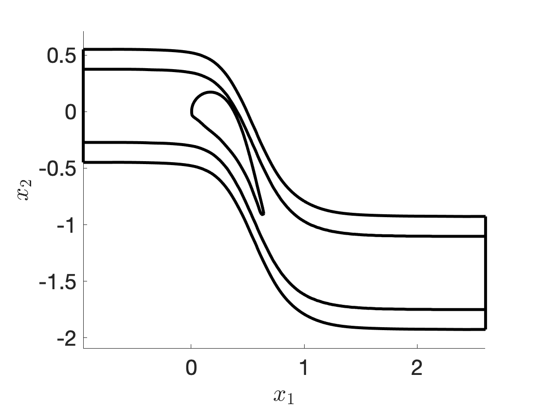
(a)

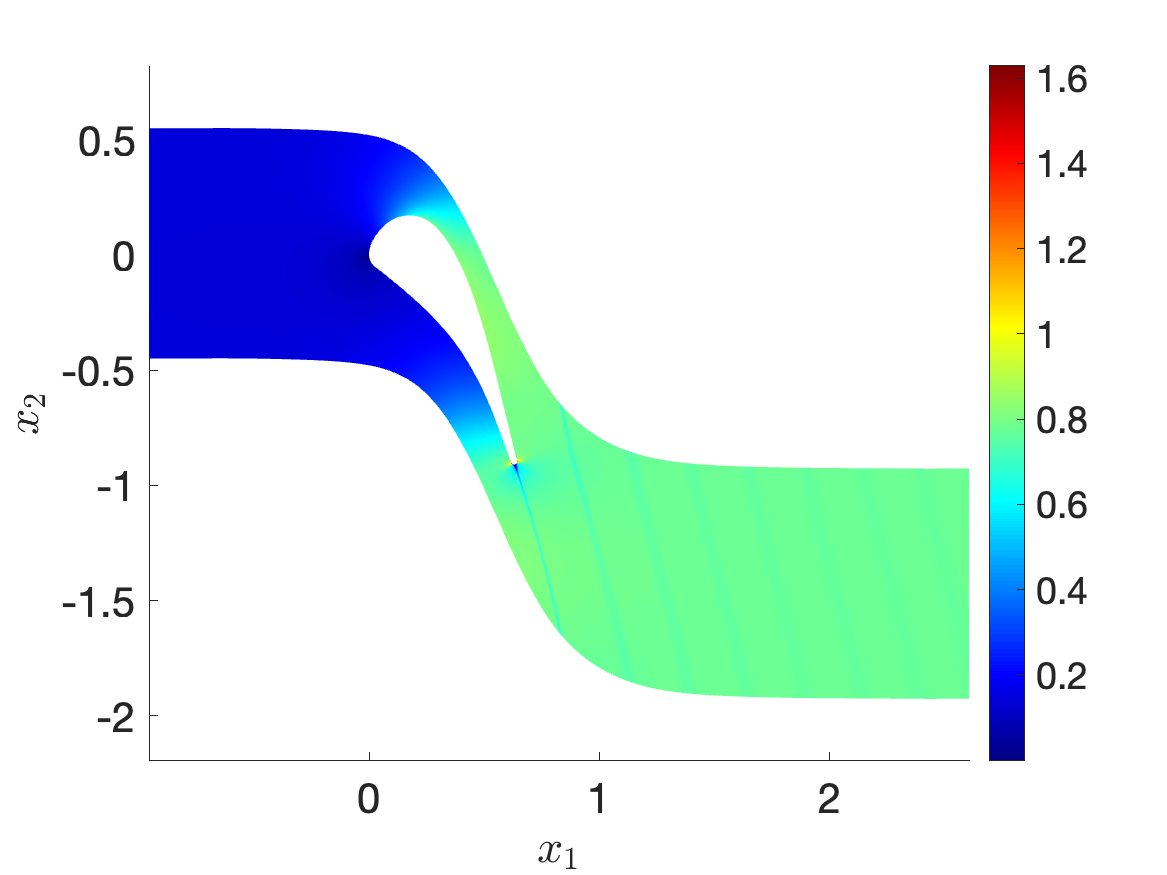
(b)

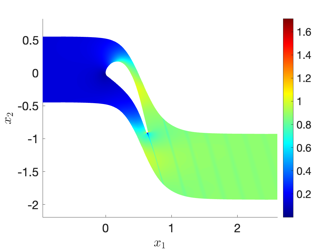
(c)

Figure 1: inviscid flow past an array of LS89 turbine blades. (a) partition associated with the geometric map. (b)-(c) behavior of the Mach number for two parameter values.

4.1.2 Results

We consider a hierarchy of six P2 meshes with $N_{\rm e}=1827,2591,3304,4249,7467,16353$ elements, respectively; Figures 2(a)-(b)-(c) show three computational meshes. Figure 2(d) show maximum and mean errors between the HF solution $u_{\mu}^{{\rm hf},(6)}$ and the corresponding HF solution associated with the $i$-th mesh,

$$E_{\mu}^{(i)}=\frac{\|u_{\mu}^{{\rm hf},(i)}-u_{\mu}^{{\rm hf},(6)}\|}{\|u_{\mu}^{{\rm hf},(6)}\|},$$ (31)

over five randomly-chosen parameters in $\mathcal{P}$ . We remark that the error is measured in the reference configuration $\Omega$, which corresponds to $H=1$. We consider the $L^{2}(\Omega)$ norm $\|\bullet\|=\sqrt{\int_{\Omega}(\bullet)^{2}\,dx}$.

(a) mesh 1

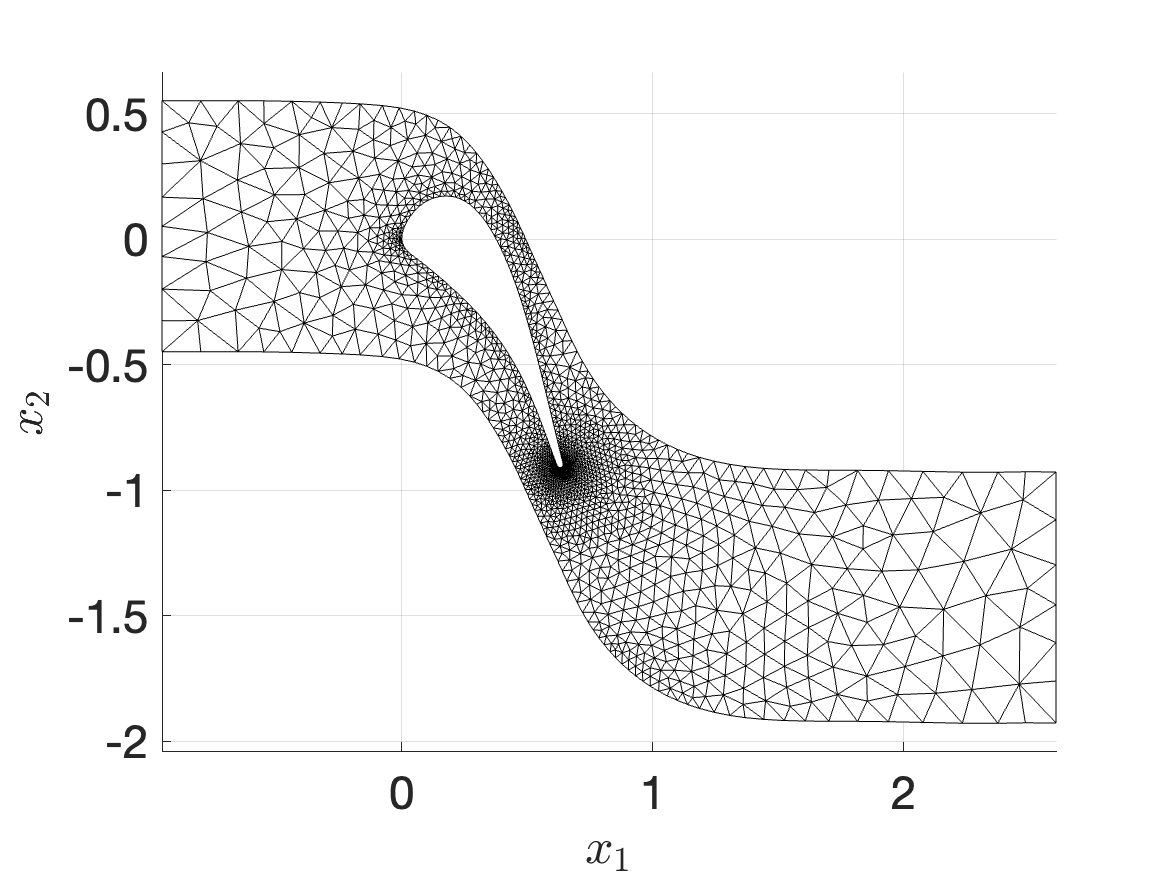
(b) mesh 3

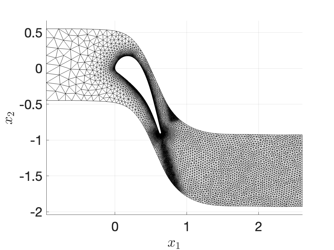
(c) mesh 6

(d)

Figure 2: compressible flow past a LS89 blade. (a)-(b)-(c) three computational meshes. (d) behavior of the average and maximum error (31).

Figure 3 compares the performance of the standard (“std”) greedy method with the performance of the incremental (“incr”) procedures of section 2.3 for the coarse mesh (mesh 1). In all the tests below, we consider a training space $\mathcal{P}_{\rm train}$ based on a ten by ten equispaced discretization of the parameter domain. Figure 3(a) shows the number of iterations of the NNLS algorithm 3, while Figure 3(b) shows the wall-clock cost (in seconds) on a commodity laptop, and Figure 3(c) shows the percentage of sampled weights $\frac{\texttt{nnz}(\boldsymbol{\rho}^{\rm eq})}{N_{\rm e}+N_{\rm f}}\times 100\%$. We observe that the proposed initialization of the active set method leads to a significant reduction of the total number of iterations, and to a non-negligible reduction of the total wall-clock cost, without affecting the performance of the method. Figure 3(d) shows the cost of constructing the test space: we notice that the progressive construction of the test space enables a significant reduction of offline costs. Finally, Figure 3(e) shows the averaged out-of-sample performance of the LSPG ROM over $n_{\rm test}=20$ randomly-chosen parameters $\mathcal{P}_{\rm test}$,

$$E_{\rm avg}=\frac{1}{n_{\rm test}}\sum_{\mu\in\mathcal{P}_{\rm test}}\frac{\|u_{\mu}^{{\rm hf},(1)}-\widehat{u}_{\mu}\|}{\|u_{\mu}^{{\rm hf},(1)}\|},$$

and Figure 3(f) shows the online costs: we observe that the standard and the incremental approaches lead to nearly-equivalent results for all values of the ROB size $n$ considered.

(a)

(b)

(c)

(d)

(e)

(f)

Figure 3: compressible flow past a LS89 blade. Progressive construction of quadrature rule and test space, coarse mesh ($N_{\rm e}=1827$).

Figure 4 replicates the tests of Figure 3 for the fine mesh (mesh 6). As for the coarser grid, we find that the progressive construction of the test space and of the quadrature rule do not hinder online performance of the LSPG ROM and ensure significant offline savings. We notice that the relative error over the test set is significantly larger: reduction of the mesh size leads to more accurate approximations of sharp features — shocks, wakes — that are troublesome for linear approximations. On the other hand, we notice that online costs are nearly the same as for the coarse mesh for the corresponding value of the ROB size $n$: this proves the effectiveness of the hyper-reduction procedure.

(a)

(b)

(c)

(d)

(e)

(f)

Figure 4: compressible flow past a LS89 blade. Progressive construction of quadrature rule and test space; fine mesh ($N_{\rm e}=16353$).

Figure 5 investigates the effectiveness of the sampling strategy based on the strong-greedy algorithm. We rely on Algorithm 6 to identify the training set of parameters $\mathcal{P}_{\star}$ for different choices of the coarse mesh $\mathcal{T}_{\rm hf}^{0}=\mathcal{T}_{\rm hf}^{(i)}$, for $i=1,\ldots,6$ and for $\mathcal{T}_{\rm hf}=\mathcal{T}_{\rm hf}^{(6)}$. Then, we measure performance in terms of the maximum relative projection error over $\mathcal{P}_{\rm train}$,

$$E_{n}^{{\rm proj},(i)}=\max_{\mu\in\mathcal{P}_{\rm train}}\inf_{\zeta\in\mathcal{Z}_{n}^{(i)}}\frac{\|u_{\mu}^{{\rm hf},(6)}-\zeta\|}{\|u_{\mu}^{{\rm hf},(6)}\|},\quad{\rm with}\;\;\mathcal{Z}_{n^{\prime}}^{(i)}={\rm span}\left\{u_{\mu}^{{\rm hf},(6)}:\mu\in\mathcal{P}_{\star,n^{\prime}}^{(i)}\right\},$$ (32)

where $\mathcal{P}_{\star,n^{\prime}}^{(i)}$ is the set of the first $n^{\prime}$ parameters selected through Algorithm 6 based on the coarse mesh $\mathcal{T}_{\rm hf}^{(i)}$. Figure 5(a) shows the behavior of the projection error $E_{n}^{{\rm proj},(i)}$ (32) for three different choices of the coarse mesh; to provide a concrete reference, we also report the performance of twenty sequences of reduced spaces obtained by randomly selecting sequences of parameters in $\mathcal{P}_{\rm train}$. Figures 5(b) and (c) show the parameters selected through Algorithm 6 for two different choices of the coarse mesh: we observe that the selected parameters are clustered in the proximity of ${\rm Ma}_{\infty}=0.9$.

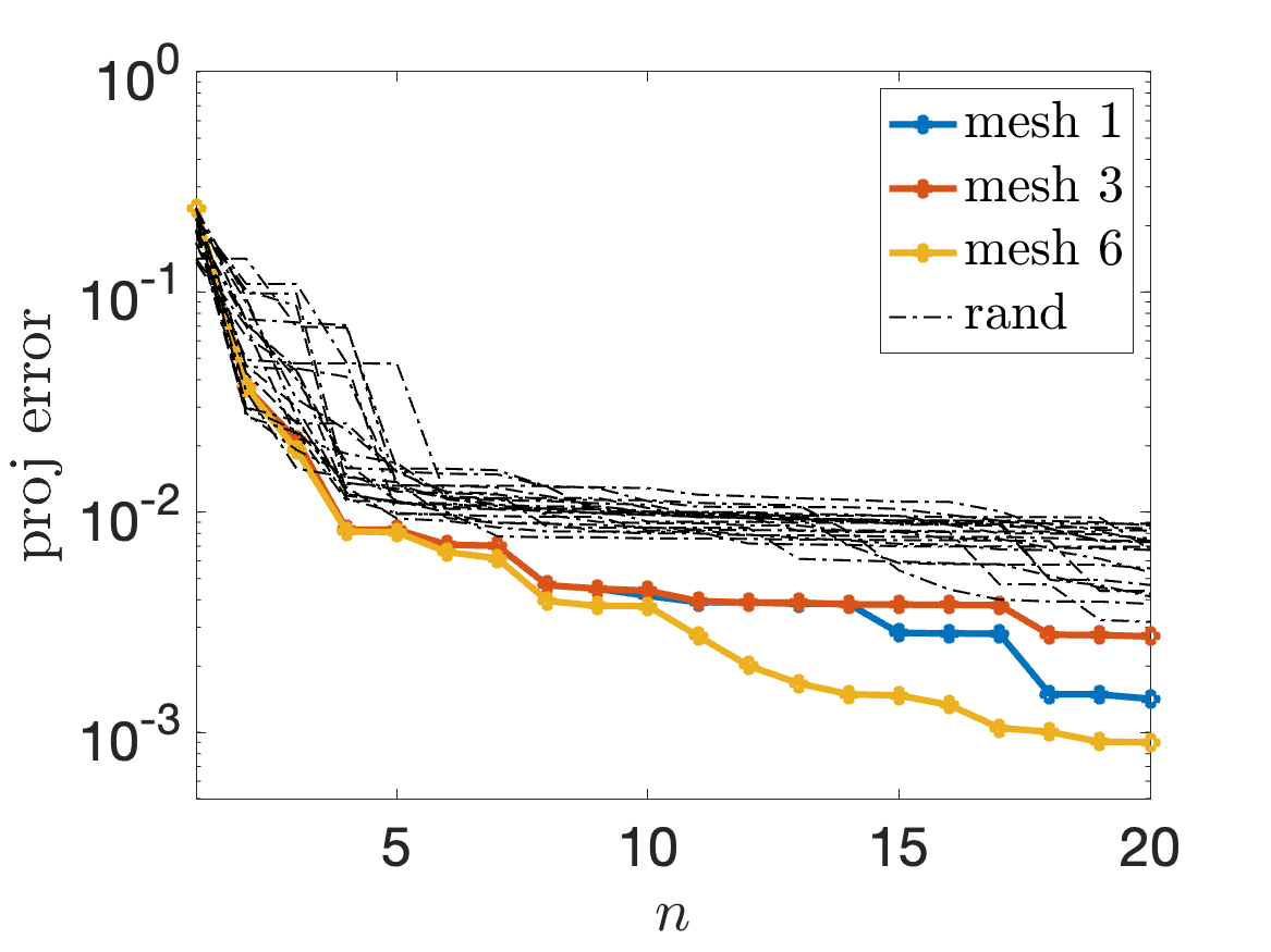
(a)

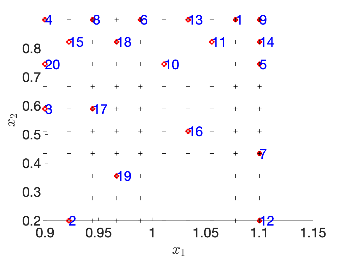
(b) mesh 1

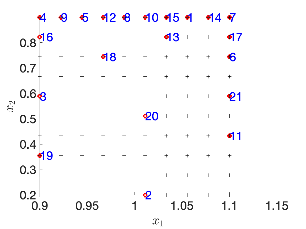
(c) mesh 6

Figure 5: compressible flow past a LS89 blade; sampling. (a) behavior of $E_{n}^{{\rm proj},(i)}$ (32) for six different choices of the coarse mesh, and for random samples. (b)-(c) parameters $\{\mu^{\star,j}\}_{j}$ selected by Algorithm 6 for two different coarse meshes.

Table 1 compares the costs of the standard weak-greedy algorithm (“vanilla”), the weak-greedy algorithm with progressive construction of the test space and the quadrature rule (“incr”), and the two-fidelity algorithm 6 with coarse mesh given by $\mathcal{T}_{\rm hf}^{0}=\mathcal{T}_{\rm hf}^{(1)}$ (“incr+MF”). To ensure a fair comparison, we impose that the final ROM has the same number of modes (twenty) for all cases. Training of the coarse ROM in Algorithm 6 is based on the weak-greedy algorithm with progressive construction of the test space and the quadrature rule, with tolerance $\texttt{tol}=10^{-3}$: this leads to a coarse ROM with $n_{0}=14$ modes, which corresponds to an initial training set $\mathcal{P}_{\star}$ of cardinality $14$ in the greedy method (cf. Line 5, Algorithm 6). The ROMs associated with three different training strategies show comparable performance in terms of online cost and $L^{2}$ errors.

fine mesh $\mathcal{T}_{\rm hf}^{(5)}$	ROB	ES	EQP	greedy search	HF solves	overhead	total
vanilla	$1.1$	$714.5$	$247.4$	$930.6$	$3554.8$	$0.6$	$5449.0$
incr	$1.1$	$177.9$	$221.2$	$928.4$	$3504.8$	$0.6$	$4834.0$
incr+MF	$0.9$	$131.0$	$121.9$	$362.7$	$2030.0$	$692.1$	$3338.5$

fine mesh $\mathcal{T}_{\rm hf}^{(6)}$	ROB	ES	EQP	greedy search	HF solves	overhead	total
vanilla	$3.4$	$2067.8$	$668.4$	$2091.2$	$10997.4$	$2.3$	$15830.5$
incr	$3.2$	$444.8$	$538.4$	$1952.8$	$10529.1$	$2.3$	$13470.6$
incr+MF	$3.6$	$366.4$	$362.5$	$905.8$	$9597.7$	$699.9$	$11935.9$

Table 1: compressible flow past a LS89 blade. Overview of offline costs for three computational strategies and two different fine meshes (coarse mesh: $\mathcal{T}_{\rm hf}^{(1)}$).

For the fine mesh $\mathcal{T}_{\rm hf}^{(6)}$, the two-fidelity training leads to a reduction of offline costs of roughly $25\%$ with respect to the vanilla implementation and of roughly $10\%$ with respect to the incremental implementation; for the fine mesh $\mathcal{T}_{\rm hf}^{(5)}$ (which has one half as many elements as the finer grid), the two-fidelity training leads to a reduction of offline costs of roughly $39\%$ with respect to the vanilla implementation and of roughly $31\%$ with respect to the incremental implementation. In particular, we notice that the initialization based on the coarse model — which is the same for both cases — is significantly more effective for the HF model associated with mesh 5 than for the HF model associated with mesh 6. The empirical finding strengthens the observation made in section 2.4 that the choice of the coarse approximation is a compromise between overhead costs — which increase as we increase the size of the coarse mesh — and accuracy of the coarse solution.

We remark that for the first two cases the HF solver is initialized using the solution for the closest parameter in the training set

$$u_{\mu^{\star,n}}^{0}=u_{\bar{\mu}}^{\rm hf},\quad{\rm with}\;\;\bar{\mu}={\rm arg}\min_{\mu^{\prime}\in\{\mu^{\star,i}\}_{i=1}^{n-1}}\|\mu^{\star,n}-\mu^{\prime}\|_{2},$$

for $n=2,3,\ldots$; for $n=1$, we rely on a coarse solver and on a continuation strategy with respect to the Mach number: this initialization is inherently sequential. On the other hand, in the two-fidelity procedure, the HF solver is initialized using the reduced-order solver that is trained using coarse HF data: this choice enables trivial parallelization of the HF solves for the initial parameter sample $\mathcal{P}_{\star}$. We hence expect to achieve higher computational savings for parallel computations.

4.2 Long-time mechanical response of the standard section of a containment building under external loading

4.2.1 Model problem

We study the long-time mechanical response of a three-dimensional standard section of a nuclear power plant containment building: the highly-nonlinear mechanical response is activated by thermal effects; its simulation requires the coupling of thermal, hydraulic and mechanical (THM) responses. A thorough presentation of the mathematical model and of the MOR procedure is provided in [4]. The ultimate goal of the simulation is to predict the temporal behavior of several quantities of interest (QoIs), such as water saturation in concrete, delayed deformations, and stresses: these QoIs are directly related to the leakage rate, whose estimate is of paramount importance for the design of NCBs. The deformation field is also important to conduct validation and calibration studies against real-world data.

Following [9], we consider a weak THM coupling procedure to model deferred deformations within the material; weak coupling is appropriate for large structures under normal operational loads. The MOR process is exclusively applied to estimate the mechanical response: the results from thermal and hydraulic calculations are indeed used as input data for the mechanical calculations, which constitute the computational bottleneck of the entire simulation workflow. To model the mechanical response of the concrete structure, we consider a three-dimensional nonlinear rheological creep model with internal variables; on the other hand, we consider a one-dimensional linear elastic model for the prestressing cables: the state variables are hence the displacement field of the three-dimensional concrete structure and of the one-dimensional steel cables. We assume that the whole structure satisfies the small-strain and small-displacement hypotheses. To establish connectivity between concrete and steel nodes, a kinematic linkage is implemented: a point within the steel structure and its corresponding point within the concrete structure are assumed to share identical displacements.

We study the solution behavior with respect to two parameters: the desiccation creep viscosity ($\eta_{\rm dc}$) and the basic creep consolidation parameter ($\kappa$) in the parameter range $\mu\in\mathcal{P}=[5\cdot 10^{8},5\cdot 10^{10}]\times[10^{-5},10^{-3}]\subset\mathbb{R}^{2}$. Figure 6 shows the behavior of (a) the normal force on a horizontal cable, and (b) the tangential and (c) vertical strains on the outer wall of the standard section of the containment building, for three distinct parameter values $\mu^{(i)}=(5.10^{9},\kappa^{(i)})$, for $\kappa^{(i)}\in\{10^{-5},10^{-4},10^{-3}\}$, $i=1,2,3$. Notation “-E” indicates that the HF data are associated to the outer face of the structure. Note that the value of the consolidation parameter $\kappa$ affects the rate of decay of the various quantities.

(a)

(b)

(c)

Figure 6: mechanical response of a NCB under external loading. (a) normal force on a horizontal cable, (b) tangential and (c) vertical strains on the outer wall of the standard section of the containment building, for $\eta_{\rm dc}=5\cdot 10^{9}$ and three values of $\kappa$ on the coarse mesh.

4.2.2 Results

High-fidelity solver. We consider the two distinct three-dimensional meshes, depicted in Figure 7: a coarse mesh of $N_{\rm e}=784$ three-dimensional hexahedral elements and a refined mesh with $N_{\rm e}=1600$ elements. This mesh features the geometry of a portion of the building halfway up the barrel, and is crossed by two vertical and three horizontal cables. We consider an adaptive time-stepping scheme: approximately 45 to 50 time steps are needed to reach the specified final time step, for all parameters in $\mathcal{P}$ and for both meshes. Table 2 provides an overview of the costs of the HF solver over the training set for the two meshes: we observe that the wall-clock cost of a full HF simulation is roughly nine minutes for the coarse mesh and seventeen minutes for the refined mesh. We consider a 7 by 7 training set $\mathcal{P}_{\rm train}$ and a 5 by 5 test set; parameters are logarithmically spaced in both directions.

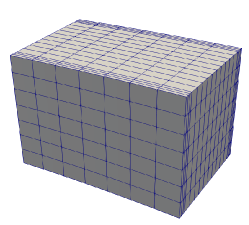
(a)

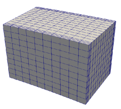
(b)

Figure 7: mechanical response of a NCB under external loading. Tridimensional meshes (HEXA20) used for code$\_$aster calculations: (a) coarse mesh (mesh 1: $N_{\rm e}=784$); (b) refined mesh (mesh 2: $N_{\rm e}=1600$).

	mean	max	min	Q1	median	Q3
mesh 1	546.91	905.53	386.96	387.04	387.12	387.19
mesh 2	1034.07	1658.53	747.60	748.20	749.78	749.40

Table 2: mechanical response of a NCB under external loading. HF CPU cost in seconds [s] for the HF simulations on the coarse (mesh 1) and the refined mesh (mesh 2)

Figure 8 showcases the evolution of normal forces in the central horizontal cable ($N_{\rm H2}$), the vertical ($\varepsilon_{zz}$) and the tangential ($\varepsilon_{tt}$) deformations on the outer surface of the geometry. Table 3 shows the behavior of the maximum and average relative errors

$$E_{\mu}^{\rm max}=\frac{\max_{k=1,\ldots,K}|q_{\mu}^{\rm hf,(1)}(t^{(k)})-q_{\mu}^{\rm hf,(2)}(t^{(k)})|}{\max_{k=1,\ldots,K}|q_{\mu}^{\rm hf,(2)}(t^{(k)})|},\quad E_{\mu}^{\rm avg}=\frac{\sum_{k=1}^{K}\Delta t^{(k)}|q_{\mu}^{\rm hf,(1)}(t^{(k)})-q_{\mu}^{\rm hf,(2)}(t^{(k)})|\,dt}{\sum_{k=1}^{K}|q_{\mu}^{\rm hf,(2)}(t^{(k)})|}.$$ (33)

for the three quantities of interest of Figure 8. We notice that the two meshes lead to nearly-equivalent results for this model problem.

(a)

(b)

(c)

Figure 8: mechanical response of a NCB under external loading. Comparison of the quantities of interest computed for the two meshes of the standard section: (a) normal force on a horizontal cable, (b) tangential and (c) vertical strains on the outer wall of the standard section of the containment building.

	$\max\limits_{\mu\in\mathcal{P}_{\rm train}}E^{\rm max}_{\mu}(\cdot)$	$E^{\rm max}_{\mu}(\cdot)/n_{\rm train}$	$\max\limits_{\mu\in\mathcal{P}_{\rm train}}E^{\rm avg}_{\mu}(\cdot)$	$E^{\rm avg}_{\mu}(\cdot)/n_{\rm train}$
$N_{\rm H2}$	$2.86\cdot 10^{-2}$	$6.55\cdot 10^{-4}$	$2.86\cdot 10^{-2}$	$3.91\cdot 10^{-5}$
$\varepsilon_{tt}-E$	$4.42\cdot 10^{-2}$	$7.68\cdot 10^{-3}$	$7.87\cdot 10^{-3}$	$4.84\cdot 10^{-3}$
$\varepsilon_{zz}-E$	$5.03\cdot 10^{-2}$	$1.09\cdot 10^{-2}$	$1.38\cdot 10^{-2}$	$6.73\cdot 10^{-3}$

Table 3: mechanical response of a NCB under external loading. Computation of average (column 1 and 3) and maximum (column 2 and 4) errors over the training set for several errors on the quantities of interest: maximum error over all time steps (cf. (33)).

Model reduction. We assess the performance of the Galerkin ROM over training and test sets. Given the sequence of parameters $\{\mu^{\star,it}\}_{it=1}^{\texttt{maxit}}$, for $it=1,\ldots,\texttt{maxit}$,

1. we solve the HF problem to find the trajectory $\{u_{\mu^{\star,it}}^{(k)}\}_{k=1}^{K}$;

2. we update the reduced space $\mathcal{Z}$ using (28) with tolerance $tol=10^{-5}$;

3. we update the quadrature rule using the (incremental) strategy described in section 3.

Below, we assess (i) the effectiveness of the incremental strategy for the construction of the quadrature rule, and (ii) the impact of the sampling strategy on performance. Towards this end, we compute the projection error

$$E_{it}^{\rm proj}(\mathcal{P}_{\bullet})=\max_{\mu\in\mathcal{P}_{\bullet}}\frac{{\left|\kern-1.07639pt\left|\kern-1.07639pt\left|\mathbb{u}_{\mu}-\Pi_{\mathcal{Z}_{it}}\mathbb{u}_{\mu}\right|\kern-1.07639pt\right|\kern-1.07639pt\right|}}{{\left|\kern-1.07639pt\left|\kern-1.07639pt\left|\mathbb{u}_{\mu}\right|\kern-1.07639pt\right|\kern-1.07639pt\right|}},\quad\bullet\in\{\rm train,\rm test\}$$ (34)

where $\Pi_{\mathcal{Z}_{it}}\mathbb{u}_{\mu}:=\{\Pi_{\mathcal{Z}_{it}}{u}_{\mu}^{(k)}\}$ and ${\left|\kern-1.07639pt\left|\kern-1.07639pt\left|\mathbb{v}\right|\kern-1.07639pt\right|\kern-1.07639pt\right|}=\sqrt{\sum_{k=1}^{K}\;\Delta t^{(k)}\|v^{(k)}\|^{2}}$ is the discrete $L^{2}(0,T;\|\cdot\|)$ norm — as in [4], we consider $\|\bullet\|=\|\bullet\|_{2}$. Further results on the prediction error and online speedups of the ROM are provided in [4].

Figure 9 illustrates the performance of the EQ procedure; in this test, we consider the finer mesh (mesh 2), and we select the parameters $\{\mu^{\star,it}\}_{it=1}^{\texttt{maxit}=15}$ using the POD-strong greedy algorithm 7 based on the HF results on mesh 1. Figures 9(a)-(b)-(c) show the number of iterations required by Algorithm 3 to meet the convergence criterion, the computational cost, and the percentage of sampled elements, which is directly related to the online costs, for $\delta=10^{-4}$. As for the previous test case, we observe that the progressive construction of the quadrature rule drastically reduces the NNLS iterations without hindering performance. Figure 9(d) shows the speedup of the incremental method for three choices of the tolerance $\delta$ and for several iterations of the iterative procedure. We notice that the speedup increases as the iteration count increases: this can be explained by observing that the percentage of new columns added during the $it$-th step in the matrix $\mathbf{G}$ decays with $it$ (cf. (29)). We further observe that the speedup increase as we decrease the tolerance $\delta$: this is justified by the fact that the number of iterations required by Algorithm 3 increases as we decrease $\delta$.

(a) $\delta=10^{-4}$

(b) $\delta=10^{-4}$

(c) $\delta=10^{-4}$

(d)

Figure 9: mechanical response of a NCB under external loading. Progressive construction of the quadrature rule on mesh 2. (a)-(b)-(c) performance of standard (“std”) and incremental (“incr”) EQ procedures for several iterations of the greedy procedures, for $\delta=10^{-4}$. (d) computational speedup for three choices of the tolerance $\delta$.

Figures 10 and 11 investigate the efficacy of the greedy sampling strategy. Figure 10 shows the parameters $\{\mu^{\star,j}\}_{j}$ selected by Algorithm 7 for (a) the coarse mesh (mesh 1) and (b) the refined mesh (mesh 2): we observe that the majority of the sampled parameters are clustered in the bottom left corner of the parameter domain for both meshes. Figure 11 shows the performance (measured through the projection error (34)) of the two samples depicted in Figure 10 on training and test sets; to provide a concrete reference, we also compare performance with five randomly-generated samples. Interestingly, we observe that for this model problem the choice of the sampling strategy has little effects on performance; nevertheless, also in this case, the greedy procedure based on the coarse mesh consistently outperforms random sampling.

(a)

(b)

Figure 10: mechanical response of a NCB under external loading. Parameters $\{\mu^{\star,j}\}_{j}$ selected by Algorithm 7 for (a) the coarse mesh (mesh 1) and (b) the refined mesh (mesh 2).

(a) out-of-sample

(b) in-sample

(c)

Figure 11: mechanical response of a NCB under external loading. Behavior of the projection error $E_{it}^{{\rm proj}}$ (34) for parameters selected by Algorithm 7 based on coarse (mesh 1) and fine data (mesh 2); comparison with random sampling. (a) performance on $\mathcal{P}_{\rm test}$ ($5\times 5$). (b) performance on $\mathcal{P}_{\rm train}$ ($7\times 7$). (c) behavior of the basis size $n_{it}$.

5 Conclusions

The computation burden of the offline training stage remains an outstanding challenge of MOR techniques for nonlinear, non-parametrically-affine problems. Adaptive sampling of the parameter domain based on greedy methods might contribute to reduce the number of offline HF solves that is needed to meet the target accuracy; however, greedy methods are inherently sequential and introduce non-negligible overhead that might ultimately hinder the benefit of adaptive sampling. To address these issues, in this work, we proposed two new strategies to accelerate greedy methods: first, a progressive construction of the ROM based on HAPOD to speed up the construction of the empirical test space for LSPG ROMs and on a warm start of the NNLS algorithm to determine the empirical quadrature rule; second, a two-fidelity sampling strategy to reduce the number of expensive greedy iterations.

The numerical results of section 4 illustrate the effectiveness and the generality of our methods for both steady and unsteady problems. First, we found that the warm start of the NNLS algorithm enables a non-negligible reduction of the computational cost without hindering performance. Second, we observed that the sampling strategy based on coarse data leads to near-optimal performance: this result suggests that multi-fidelity algorithms might be particularly effective to explore the parameter domain in the MOR training phase.

The empirical findings of this work motivate further theoretical and numerical investigations that we wish to pursue in the future. First, we wish to analyze the performance of multi-fidelity sampling methods for MOR: the ultimate goal is to devise a priori and a posteriori indicators to drive the choice of the mesh hierarchy and the cardinality $n_{0}$ of the set $\mathcal{P}_{\star}$ in Algorithm 6. Second, we plan to extend the two elements of our formulation — progressive ROM generation and multi-fidelity sampling — to optimization problems for which the primary objective of model reduction is to estimate a suitable quantity of interest (goal-oriented MOR): in this respect, we envision to combine our formulation with adaptive techniques for optimization [40, 5, 37].

Acknowledgements.

This work was partly funded by ANRT (French National Association for Research and Technology) and EDF. The authors thank Dr. Jean-Philippe Argaud, Dr. Guilhem Ferté (EDF R&D) and Dr. Michel Bergmann (Inria Bordeaux) for fruitful discussions. The first author thanks the code aster development team for fruitful discussions on the FE software employed for the numerical simulations of section 4.2.

Data availability statement.

The data that support the findings of this study are available from the corresponding author, TT, upon reasonable request. The software developed for the investigations of section 4.2 is expected to be integrated in the open-source Python library Mordicus [2], which is funded by a “French Fonds Unique Interministériel” (FUI) project.

References

- [1] Finite element codeaster, Analysis of Structures and Thermomechanics for Studies and Research. Electricité de France (EDF), Open source on www.code-aster.org, 1989-2024.
- [2] Mordicus Python package. Consortium of the FUI project MOR DICUS. Electricité de France (EDF), Open source on https://gitlab.com/mor dicus/mordicus, 2022.
- [3] E. Agouzal, J.-P. Argaud, M. Bergmann, G. Ferté, and T. Taddei. A projection-based reduced-order model for parametric quasi-static nonlinear mechanics using an open-source industrial code. International Journal for Numerical Methods in Engineering, accepted, 2023.
- [4] E. Agouzal, J.-P. Argaud, M. Bergmann, G. Ferté, and T. Taddei. Projection-based model order reduction for prestressed concrete with an application to the standard section of a nuclear containment building. arXiv preprint arXiv:2401.05098, 2024.
- [5] N. M. Alexandrov, R. M. Lewis, C. R. Gumbert, L. L. Green, and P. A. Newman. Approximation and model management in aerodynamic optimization with variable-fidelity models. Journal of Aircraft, 38(6):1093–1101, 2001.
- [6] N. Barral, T. Taddei, and I. Tifouti. Registration-based model reduction of parameterized PDEs with spatio-parameter adaptivity. Journal of Computational Physics, page 112727, 2023.
- [7] M. Barrault, Y. Maday, N. C. Nguyen, and A. T. Patera. An ‘empirical interpolation’method: application to efficient reduced-basis discretization of partial differential equations. Comptes Rendus Mathematique, 339(9):667–672, 2004.
- [8] A. Benaceur, V. Ehrlacher, A. Ern, and S. Meunier. A progressive reduced basis/empirical interpolation method for nonlinear parabolic problems. SIAM Journal on Scientific Computing, 40(5):A2930–A2955, 2018.
- [9] D. Bouhjiti. Analyse probabiliste de la fissuration et du confinement des grands ouvrages en béton armé et précontraint-application aux enceintes de confinement des réacteurs nucléaires (cas de la maquette vercors). Academic Journal of Civil Engineering, 36(1):464–471, 2018.
- [10] M. Brand. Fast online svd revisions for lightweight recommender systems. In Proceedings of the 2003 SIAM international conference on data mining, pages 37–46. SIAM, 2003.
- [11] K. Carlberg, C. Farhat, J. Cortial, and D. Amsallem. The GNAT method for nonlinear model reduction: effective implementation and application to computational fluid dynamics and turbulent flows. Journal of Computational Physics, 242:623–647, 2013.
- [12] F. Casenave, N. Akkari, F. Bordeu, C. Rey, and D. Ryckelynck. A nonintrusive distributed reduced-order modeling framework for nonlinear structural mechanics—application to elastoviscoplastic computations. International journal for numerical methods in engineering, 121(1):32–53, 2020.
- [13] T. Chapman, P. Avery, P. Collins, and C. Farhat. Accelerated mesh sampling for the hyper reduction of nonlinear computational models. International Journal for Numerical Methods in Engineering, 109(12):1623–1654, 2017.
- [14] A. Cohen and R. DeVore. Approximation of high-dimensional parametric PDEs. Acta Numerica, 24:1–159, 2015.
- [15] P. Conti, M. Guo, A. Manzoni, A. Frangi, S. L. Brunton, and J. N. Kutz. Multi-fidelity reduced-order surrogate modeling. arXiv preprint arXiv:2309.00325, 2023.
- [16] E. Du and M. Yano. Efficient hyperreduction of high-order discontinuous Galerkin methods: element-wise and point-wise reduced quadrature formulations. Journal of Computational Physics, 466:111399, 2022.
- [17] C. Farhat, P. Avery, T. Chapman, and J. Cortial. Dimensional reduction of nonlinear finite element dynamic models with finite rotations and energy-based mesh sampling and weighting for computational efficiency. International Journal for Numerical Methods in Engineering, 98(9):625–662, 2014.
- [18] C. Farhat, T. Chapman, and P. Avery. Structure-preserving, stability, and accuracy properties of the energy-conserving sampling and weighting method for the hyper reduction of nonlinear finite element dynamic models. International journal for numerical methods in engineering, 102(5):1077–1110, 2015.
- [19] L. Feng, L. Lombardi, G. Antonini, and P. Benner. Multi-fidelity error estimation accelerates greedy model reduction of complex dynamical systems. International journal for numerical methods in engineering, 124(3):5312–5333, 2023.
- [20] B. Haasdonk. Reduced basis methods for parametrized PDEs–a tutorial introduction for stationary and instationary problems. Model reduction and approximation: theory and algorithms, 15:65, 2017.
- [21] B. Haasdonk and M. Ohlberger. Reduced basis method for finite volume approximations of parametrized linear evolution equations. ESAIM: Mathematical Modelling and Numerical Analysis, 42(2):277–302, 2008.
- [22] J. A. Hernandez, M. A. Caicedo, and A. Ferrer. Dimensional hyper-reduction of nonlinear finite element models via empirical cubature. Computer methods in applied mechanics and engineering, 313:687–722, 2017.
- [23] C. Himpe, T. Leibner, and S. Rave. Hierarchical approximate proper orthogonal decomposition. SIAM Journal on Scientific Computing, 40(5):A3267–A3292, 2018.
- [24] A. Iollo, G. Sambataro, and T. Taddei. An adaptive projection-based model reduction method for nonlinear mechanics with internal variables: Application to thermo-hydro-mechanical systems. International Journal for Numerical Methods in Engineering, 123(12):2894–2918, 2022.
- [25] C. L. Lawson and R. J. Hanson. Solving least squares problems. SIAM, 1995.
- [26] MATLAB. R2022a. The MathWorks Inc., Natick, Massachusetts, 2022.
- [27] A. Paul-Dubois-Taine and D. Amsallem. An adaptive and efficient greedy procedure for the optimal training of parametric reduced-order models. International Journal for Numerical Methods in Engineering, 102(5):1262–1292, 2015.
- [28] A. Quarteroni, A. Manzoni, and F. Negri. Reduced basis methods for partial differential equations: an introduction, volume 92. Springer, 2015.
- [29] D. Ryckelynck. Hyper-reduction of mechanical models involving internal variables. International Journal for numerical methods in engineering, 77(1):75–89, 2009.
- [30] L. Sirovich. Turbulence and the dynamics of coherent structures. I. Coherent structures. Quarterly of applied mathematics, 45(3):561–571, 1987.
- [31] T. Taddei. Compositional maps for registration in complex geometries. arXiv preprint arXiv:2308.15307, 2023.
- [32] T. Taddei and L. Zhang. Space-time registration-based model reduction of parameterized one-dimensional hyperbolic PDEs. ESAIM: Mathematical Modelling and Numerical Analysis, 55(1):99–130, 2021.
- [33] K. Urban and A. Patera. An improved error bound for reduced basis approximation of linear parabolic problems. Mathematics of Computation, 83(288):1599–1615, 2014.
- [34] K. Veroy, C. Prud’Homme, D. Rovas, and A. Patera. A posteriori error bounds for reduced-basis approximation of parametrized noncoercive and nonlinear elliptic partial differential equations. In 16th AIAA Computational Fluid Dynamics Conference, page 3847, 2003.
- [35] S. Volkwein. Model reduction using proper orthogonal decomposition. Lecture Notes, Institute of Mathematics and Scientific Computing, University of Graz. see http://www. uni-graz. at/imawww/volkwein/POD. pdf, 1025, 2011.
- [36] M. Yano. Discontinuous Galerkin reduced basis empirical quadrature procedure for model reduction of parametrized nonlinear conservation laws. Advances in Computational Mathematics, 45(5):2287–2320, 2019.
- [37] M. Yano, T. Huang, and M. J. Zahr. A globally convergent method to accelerate topology optimization using on-the-fly model reduction. Computer Methods in Applied Mechanics and Engineering, 375:113635, 2021.
- [38] M. Yano, J. Modisette, and D. Darmofal. The importance of mesh adaptation for higher-order discretizations of aerodynamic flows. In 20th AIAA Computational Fluid Dynamics Conference, page 3852, 2011.
- [39] M. Yano and A. T. Patera. An LP empirical quadrature procedure for reduced basis treatment of parametrized nonlinear PDEs. Computer Methods in Applied Mechanics and Engineering, 344:1104–1123, 2019.
- [40] M. J. Zahr and C. Farhat. Progressive construction of a parametric reduced-order model for PDE-constrained optimization. International Journal for Numerical Methods in Engineering, 102(5):1111–1135, 2015.