Graph Language Models

Abstract

While Language Models have become workhorses for NLP, their interplay with textual knowledge graphs (KGs) – structured memories of general or domain knowledge – is actively researched. Current embedding methodologies for such graphs typically either (i) linearize graphs for embedding them using sequential Language Models (LMs), which underutilize structural information, or (ii) use Graph Neural Networks (GNNs) to preserve graph structure, while GNNs cannot represent textual features as well as a pre-trained LM could. In this work we introduce a novel language model, the Graph Language Model (GLM), that integrates the strengths of both approaches, while mitigating their weaknesses. The GLM parameters are initialized from a pretrained LM, to facilitate nuanced understanding of individual concepts and triplets. Simultaneously, its architectural design incorporates graph biases, thereby promoting effective knowledge distribution within the graph. Empirical evaluations on relation classification tasks on ConceptNet subgraphs reveal that GLM embeddings surpass both LM- and GNN-based baselines in supervised and zero-shot settings.

1 Introduction

Knowledge Graphs (KGs) play a crucial role in information representation and retrieval, offering a structured framework to organize and connect vast data. KGs excel in making manifold relationships explicit, empowering organizations and researchers to unlock hidden insights and enhanced information retrieval for improved decision-making. As the data landscape expands, KGs become essential for navigating and harnessing the wealth of information in the digital age, enabling the discovery of unseen connections within and across complex data sources, ultimately driving innovation.

Language models (LMs) have demonstrated remarkable proficiency in various NLP tasks, showcasing their capabilities in analyzing and generating text. However, they are predominantly confined to processing sequential data, such as sentences or paragraphs, which limits their ability to effectively handle graph-based data. I.e., graphs – consisting of nodes and edges that represent relationships and interactions in a non-linear way – present a challenge that goes beyond the sequential structure of natural language.

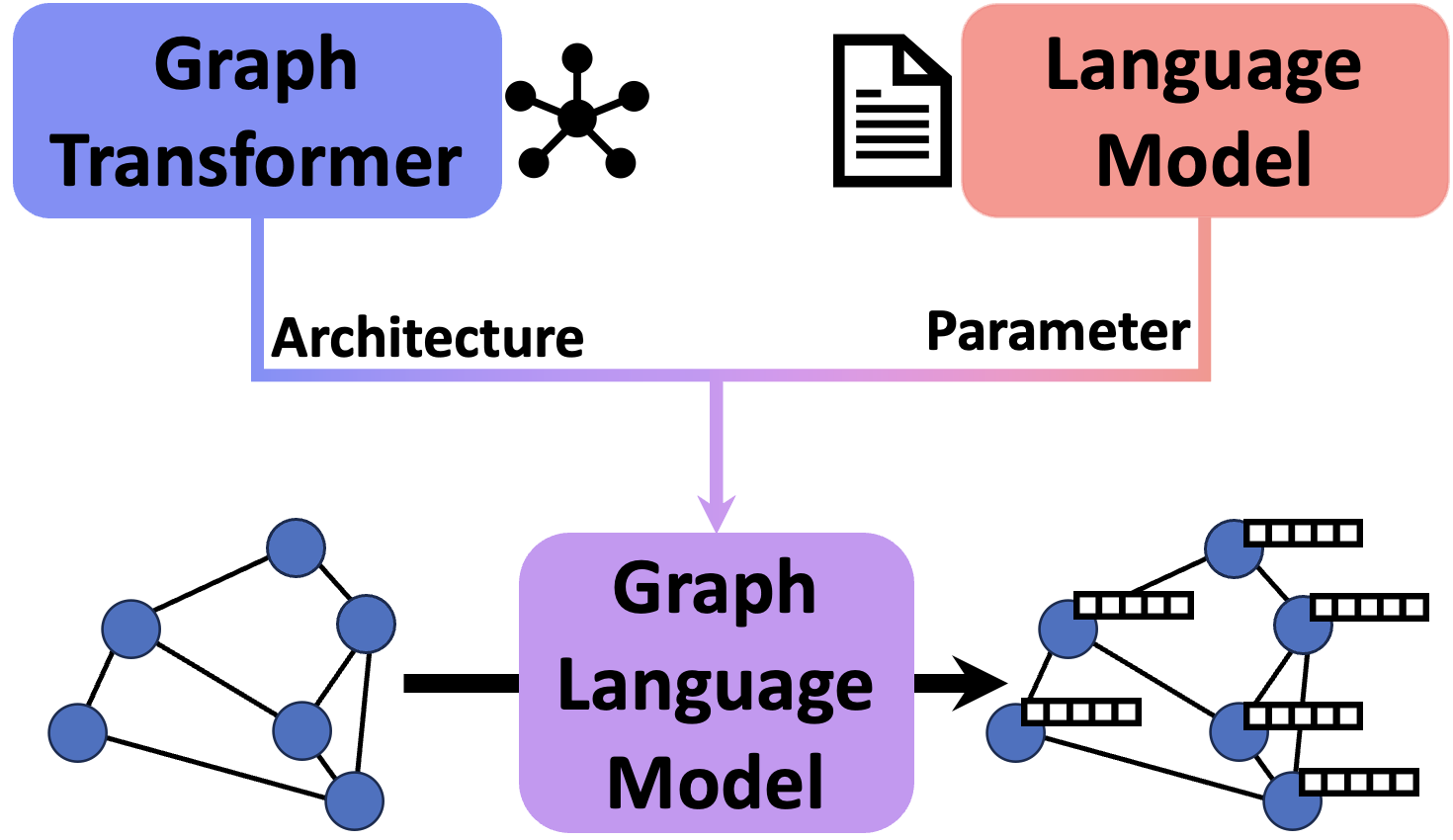
Figure 1: The GLM inherits its architecture from a Graph Transformer, and its parameters from a LM. This enables it to jointly reason over graphs and language.

Many KGs consist of a collection of knowledge triplets, where nodes are entities and edges represent relations holding between these entities. Each triplet represents a fact, e.g., (dog; IsA; animal) in ConceptNet (Speer et al., 2017) or (Thailand; Capital; Bankok) in DBpedia (Auer et al., 2007). Despite the (usual) simplicity of each triplet individually, complex structures emerge when triplets are combined in a KG. Such Graphs of Triplets (GoT) are common representations for KGs.

For effectively using GoTs, we need meaningful encodings of their components. A natural choice is leveraging LMs, as they can capture the semantic content of textually encoded entities, relations or entire triplets. However, LMs are not inherently prepared to capture graph-structured information, which is crucial to capture interactions in a GoT. To alleviate this problem, we can leverage graph NNs (GNNs). GNNs, on the other hand, are not well prepared to capture meanings associated with text, and hence often LMs are used to convert nodes (and potentially edges) to language-based semantic embeddings. But in such settings, semantic encoding leveraged from LMs and structural reasoning performed by GNNs are separated and are driven by distinct underlying principles. We expect this to limit model performance if both, semantic and structural information, are important for a task.

To enable early fusion of semantic and structural information, we propose a new Graph Language Model (GLM) formulation. The most powerful LMs today are transformer-based. Since transformers operate on sets, so-called Positional Encoding (PE) is used to make them sensitive to the inherent sequential ordering of linguistic inputs. In our GLM formulation, we modify PE and self-attention to convert LMs (i.e., sequence transformers) to graph transformers that natively operate on graphs, while preserving their LM capabilities. Usually, a new model architecture requires pretraining from scratch, which is extremely costly. By creating a new architecture that unifies relevant features of the LM and Graph Transformer (GT) architectures, we can continue using the pretrained parameters of the LM. This is possible since we adopt some non-invasive changes in the self-attention module: We define LM-like attention patters for the processing of linearly organized textual information, and GT-like attention patterns for information aggregation in the graph. Hence, our proposed GLM inherits semantic understanding of entities and triplets from the LM, while architectural features assimilated from the GT allow it to directly perform structural reasoning, without relying on external GNN layers.

Our contributions are: (i) We propose Graph Language Models (GLMs) and offer a theoretical framework to construct them. GLMs are graph transformers, which enables graph reasoning. Simultaneously, they integrate elements of the transformer LM architecture, which allows them to effectively represent and contextualize triplets inside a GoT. (ii) Experiments on relation classification in ConceptNet subgraphs show that GLMs outperform LM- and GNN-based methods for encoding GoTs – even when LM parameters are not updated to adapt to the new architecture in the GLM. (iii) Ablations confirm that weight initialization from a LM is crucial for the GLM’s high performance.

2 Preliminary: Graph Transformers

This section gives a brief overview of graph transformers (GTs), focusing on architectural choices relevant for our work. We refer to Min et al. (2022) for a detailed overview of GTs. As GTs are a type of GNN, we also discuss some general properties of GNNs that motivate our design choices in §3.

The attention mechanism in self-attention can be written as

$$\textrm{Softmax}\left(\frac{QK^{T}}{\sqrt{d}}+B_{P}+M\right)V,$$ (1)

where $Q$, $K$ and $V$ are the query, key and value matrices, and $d$ is the query and key dimension (Vaswani et al., 2017). $B_{P}$ and $M$ are matrices which can be used for positional encoding and masking, respectively. Setting $B_{P}=M=0$ yields the formulation in Vaswani et al. (2017). We will discuss the roles of $B_{P}$ and $M$ for GTs below.

Positional Encoding

The Self-Attention mechanism of transformer models is permutation invariant, i.e., it doesn’t have any notion of the order of elements in its input. Positional Encoding (PE) is commonly used to inform LMs on the ordering of tokens in a sentence (Dufter et al., 2022). Most approaches employ either absolute PE, where absolute token positions are encoded (Vaswani et al., 2017; Gehring et al., 2017) or relative PE, which encodes the relative position between pairs of tokens (Shaw et al., 2018; Raffel et al., 2020; Su et al., 2021; Press et al., 2022). Absolute PE are typically combined with the input sequence and hence, the PE does not need to be encoded in self-attention ($B_{P}=0$). In relative PE $B_{P}$ is used to encode a bias depending on the relative distances between pairs of tokens – for example, by learning one scalar for each possible distance:

$$B_{P}=f(P),$$ (2)

where $P$ is a matrix of relative distances and $f(\cdot)$ an elementwise function. Some approaches are orthogonal to this classification and can be combined with either one (Ke et al., 2021; Ruoss et al., 2023).

Similarly, GTs use PEs to encode the structure of the input, and hence, their PE has to encode a graph structure, as opposed to a sequence. This can again be done with absolute or relative PEs. However, defining an “absolute position” of a node or edge in a graph is not straightforward. While many methods exist, they are not directly compatible with the usual (absolute) “counting position” known from sequence encoding in LMs. We therefore focus on relative PE in this work. Given a directed acyclic path in a graph, we can define the (signed) distance between any pair of nodes along a path simply as the number of hops between the nodes. The sign can be determined by the direction of the path. Thus, when we find a consistent set of such paths, we have PE for our graph. Our choice of these paths will be described in §3.

Masked Attention

In a vanilla transformer, self-attention is computed for all possible pairs of tokens in the input. By contrast, nodes typically only attend to adjacent nodes in GNNs. Therefore, information between more distant nodes has to be propagated across multiple GNN layers. For graphs, such sparse message passing approaches are sometimes preferred, as in most graphs the neighborhood size increases exponentially with increasing radius, which can cause loss of information due to over-smoothing (Chen et al., 2020). Thus, in GTs it can be beneficial to introduce graph priors, for example by restricting self-attention to local neighborhoods. This can be realized by setting elements of $M$ to $0$ for pairs of tokens that should be connected, and to $-\infty$ otherwise.

On the other hand, it has been shown that a global view of the graph can enable efficient, long-ranged information flow (Alon and Yahav, 2021; Ribeiro et al., 2020). We will therefore present two model variants – a local and a global GLM.

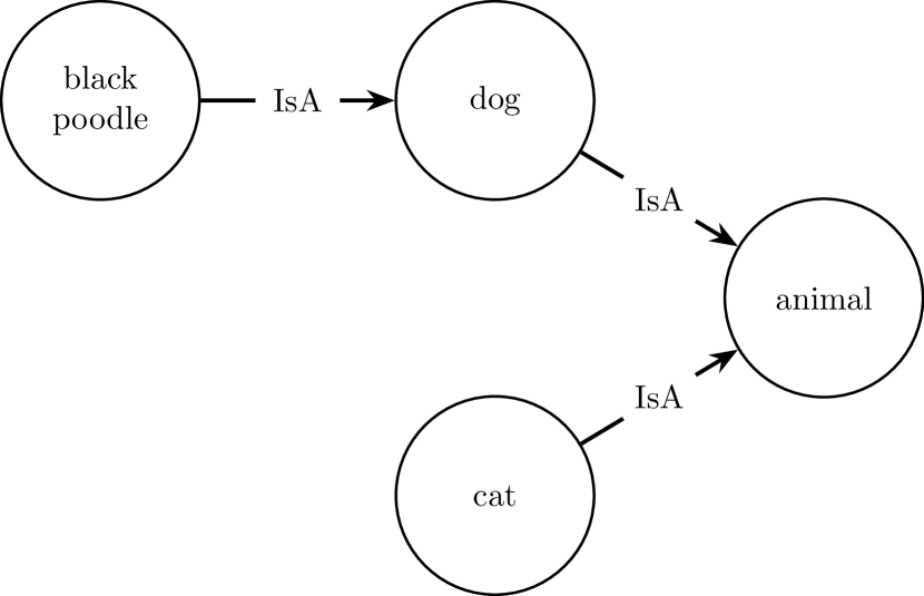
(a) Original GoT

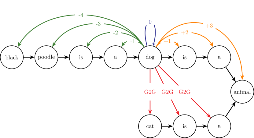
(b) Extended Levi graph of GoT (with relative distances $P$ for dog)

Figure 2: Example of graph preprocessing in our GLM. Fig 2(b) shows relative distances for dog, i.e., when dog is attending to other tokens. The red Graph-to-Graph (G2G) connections only exist for the $g$GLM, not for the $\ell$GLM.

3 Graph Language Model

GLM vs. GT

We aim to design an architecture that can efficiently and jointly reason over textual and graph-structured data. GTs are a special type of GNN (cf. §2 and Bronstein et al. (2021)), and hence can offer the desired graph priors. Yet, they lack language understanding, as they are not equipped with knowledge that LMs acquire during pretraining on textual data.

One intuitive approach allowing to bridge this gap is to pretrain a GT from scratch (Schmitt et al., 2021). But large-scale pretraining is costly and the necessary data is bound to be scarce. We therefore take a different avenue. We hypothesize that the language understanding capabilities required for reasoning over GoTs is similar to the reasoning performed when processing sequential texts. Intuitively this should be the case, since (i) GoTs are designed to be understandable by humans and (ii) literate people can ‘read’ and understand GoTs. Existing LMs have such language understanding capability stored in their parameters.

By initializing a GT with parameters from a compatible LM, we obtain our Graph Language Model (GLM). The GT architecture introduces graph priors, while the parameter initialization from the LM introduces textual understanding. In the following we explain the necessary modifications to the input graph and to the model, to make this work. The general idea is that (verbalized) triplets should resemble natural language as much as possible to enable LM weights to capture them, while graph reasoning should be done via message passing.

Graph preprocessing

A LM tokenizer converts text into a sequence of tokens, which the LM can then process. In a similar way, we need to process GoTs, such that the GLM can process the graphs “as a LM would do” (cf. Fig. 2). To achieve this, we first convert the GoT to its so-called Levi graph (Schmitt et al., 2021), i.e., we replace each edge with a node that contains the relation name as textual feature, and connect the new node to the head and tail of the original edge via unlabeled edges, preserving the directionality of the original edge. If necessary, we verbalize the relation: for example, for ConceptNet (CN) we convert the relation label IsA to the natural language expression is a. Next, we tokenize each node using the tokenizer of the underlying LM. Finally, we split each node into multiple nodes, such that every new node contains a single token, and connect adjacent nodes via edges, again preserving the directionality of the original relation. This yields the final extended Levi graph (see Fig. 2(b)).

In this representation, each triplet is formalized as a sequence of tokens – just as it would be for a standard LM. The representation is thus well-suited for the GLM to seamlessly process of the original graph nodes and labels.

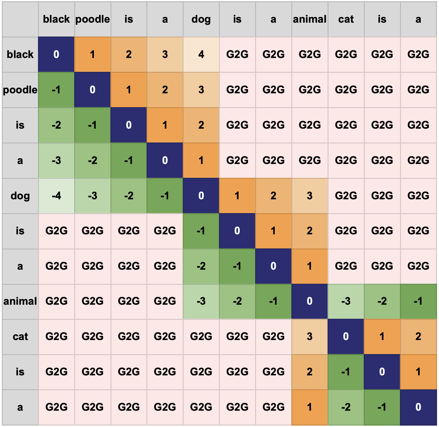
Figure 3: Relative position matrix $P$ for tokens in Fig. 2(b). Entries with G2G either have no relative position ($\ell$GLM) or a relative position of $\infty$ ($g$GLM) (cf. Appendix, Fig. 4).

Positional Encodings

As discussed in §2, we prefer PEs that encode the relative position between pairs of tokens, determined by their signed distance. We can directly adopt this method to encode the relative position of pairs of tokens occurring within the same triplet – by simply considering the triplet as a piece of text, and counting the token distance in this text. Note that a single token can occur in multiple triplets, having, e.g., multiple “lefthand side neighbors” (cf. animal in Fig. 2(b) and 3). While this does not occur in ordinary sequential text, it does not impose a problem for relative PE.

Yet, for pairs of tokens that do not belong to the same triplet, we cannot follow the usual approach, since we cannot guarantee that there is a canonical text that connects the tokens. To determine the distance between such pairs of tokens belonging to different triplets, previous work considered, e.g., the length of the shortest path between them (Schmitt et al., 2021). However, this results in PEs that do not come natural to a LM, since a triplet would appear in reversed order, if a triplet is traversed in “the wrong direction” in the shortest path. We therefore omit structure-informed PE between tokens that do not belong to the same triplet and instead propose two GLM variants: a local ($\ell$GLM) and a global ($g$GLM) Graph Language Model.

Metric	$r=1$	$r=2$	$r=3$	$r=4$	$r=5$
#nodes	2.00 $\pm$ 0.00	5.77 $\pm$ 0.46	12.28 $\pm$ 1.67	23.47 $\pm$ 4.33	42.90 $\pm$ 9.57
#edges	1.00 $\pm$ 0.00	8.25 $\pm$ 2.74	19.19 $\pm$ 5.33	36.41 $\pm$ 9.09	66.06 $\pm$ 16.77
mean degree	1.00 $\pm$ 0.00	2.87 $\pm$ 0.96	3.14 $\pm$ 0.82	3.11 $\pm$ 0.59	3.08 $\pm$ 0.42

Table 1: Structural statistics of train graphs.

Local and global GLM

Fig. 3 shows the relative token position matrix $P$ for the graph in Fig. 2(b). In the $\ell$GLM the self-attention mechanism is restricted to tokens from the same triplet. This means that attention to any token located beyond the local triplet is set to $0$ – and hence does not require PE. Still, in such configurations, messages can propagate through the graph across multiple layers, since tokens belonging to a concept can be shared by multiple triplets. This is analogous to standard message passing in GNNs, where non-adjacent nodes have no direct connection, but can still share information via message passing. For example, the representation of dog is contextualized by the triplets black poodle is a dog and dog is a animal after the first $\ell$GLM layer. Hence in the second layer, when animal attends to dog, the animal embedding gets impacted by black poodle, even though there is no direct connection from animal to black poodle.

However, it has been shown that a global view can sometimes be beneficial (Ribeiro et al., 2020). Hence, we also formalize the $g$GLM, as an alternative, where self-attention can connect any node to every other node. For this setting we need to assign a PE to any pair of tokens, including those that do not occur within the same triplet. For these pairs we set the relative position to $+\infty$ in $P$. In a LM a relative PE of $+\infty$ means that the respective tokens occur somewhere “far” away in a remote text passage. LMs learn a proximity bias during pretraining, i.e., they tend to have higher attention scores between tokens that are close to each other in the text. This means that tokens with a high relative distance tend to have low attention scores. For our $g$GLM this corresponds to a graph bias where distant nodes are less important, but are still accessible. Note that unlike in the $\ell$GLM, this bias is not part of the architecture. Instead, it originates from the pretrained parameters, which means that the $g$GLM can learn to attend more to distant tokens.

Together with $P$ and $M$, the GLM takes a sequence consisting of all tokens in the extended Levi graph as input. For this, we technically need to “linearize” the graph. However, the order of tokens in the resulting sequence does not matter: relative positions in $P$ are determined by distances in the the graph, not in the sequence. Permuting the input sequence simply means that rows and columns of $P$ and $M$ need to be permuted accordingly, but the resulting token embeddings remain unchanged. Example matrices for $P$ and $M$ for the $\ell$GLM and $g$GLM are shown in Appendix, Fig. 4.

Uni- and Bidirectional LMs

If the LM’s self-attention is uni-directional, information can only be propagated in the direction of the arrows in Fig. 2(b) for the $\ell$GLM. This means that, e.g., the representation of the node black poodle is independent of the rest of the graph. In principle, we can augment the graph with inverse relations, to enable bidirectional information flow even with a unidirectional LM. In this work, however, we restrict our analysis to bidirectional models.

T5

In this work we chose T5 (Raffel et al., 2020) as base LM to instantiate the local and global GLM variants. T5 comes in various sizes and consists of a bidirectional encoder, together with a unidirectional decoder. We convert the encoder to a GLM using the steps above. In T5, the relative distances in $P$ are grouped into so-called buckets, and each bucket gets mapped to one learned positional bias in $B_{P}$ for each head. The positional biases are shared across layers. The T5 decoder is not needed to encode graphs, but could be used to generate a sequence, e.g., text or a linearized graph.

4 Experiments

4.1 Dataset

We evaluate our method on the task of relation label classification on randomly selected subgraphs from the largest connected component of the English part of ConceptNet (CN) version 5.7 (Speer et al., 2017), which consists of 125,661 concepts and 1,025,802 triplets. We select 17 distinct relation label classes (cf. Appendix, Tab. 4), ensuring sufficient frequency and semantic dissimilarity. For each class, we randomly sample 1,000 triplets, allowing only cases where exactly one triplet connects the head and tail entities, to reduce label ambiguity. These 1,000 instances are split into train (800), dev (100), and test (100). This creates a balanced dataset of 13,600 train instances, 1,700 dev instances, and 1,700 test instances. To predict relation labels, we replace them with <extra_id_0>, T5’s first mask token.

To investigate the impact of varying graph complexities, we experiment with different graph sizes of CN subgraphs. We start with a radius of $r=1$, when we consider only the two concepts (head and tail) used by the target triplet. To create a larger graph context, we randomly select 4 adjacent triplets – 2 for the head, and 2 for the tail entity of the original triplet. A graph with radius $r=2$ is formed by the subgraph spanned by all entities used in these 5 triplets. For $r=3$ we again randomly select 2 triplets for each of the outer (up to) 4 entities, yielding (up to) 13 triplets. To avoid accidentally adding more short-ranged information, we restrict the new triplets to triplets that actually extend the radius of the graph. This enables us to control graph size and complexity, while still enabling sufficient diversity in the graph structure. Further, the graphs are created such that graphs for smaller radii are strict subgraphs of graphs with larger radii. This ensures that performance changes with increasing radii are due to long-ranged connections, and not due to potentially different short-ranged information. Tab. 1 shows statistics of train graphs, depending on their radius.

The correct class label of the targeted relation mainly depends on the concepts in the original triplet. To evaluate model effectiveness when long-ranged connections are crucial, we experiment with masking complete subgraphs around the relation to be predicted. The size of the masked subgraph is denoted by $m$, where $m=0$ means no masking, $m=1$ masks neighboring concepts, $m=2$ masks neighboring concepts and the next relations, and so on. We replace each concept and relation in the masked subgraph with a different mask token.

4.2 Experimental setup

Input to the models is a CN subgraph, where the relation to be predicted is replaced with <extra_id_0>. The GLMs encode the graph as detailed in §3, producing an embedding for each token. To obtain a prediction for the masked relation label, we train a linear classification head that takes the mask’s embedding as input and predicts a probability for each of the 17 relation label classes. As discussed in §3, we verbalize unmasked relations according to static templates, shown in the Appendix, Tab. 4 (Plenz et al., 2023). This makes individual triplets more similar to natural language.

In a standard finetuning setting we train the GLM parameters and the classification head jointly. However, since the GLM is initialized from a LM, we hypothesize that it should produce meaningful embeddings, even without any training. To test this hypothesis, we train only the classification head, i.e., we only train a linear probe on the embedding we obtain from the encoded graph. Note that in this setting, the GLM was never trained on any graph data, similar to a zero-shot setting. The linear probe can only perform linear feature extraction and hence, can only achieve high performance if the GLM embeddings show expressive features without any training.

We report mean accuracy across 5 different runs. Hyperparameters, including number of trainable parameters, are shown in the Appendix, Tab. 5. Unless stated otherwise, we run our experiments with T5-small to allow for many baselines. We also run experiments with T5-base and T5-large to observe scaling with larger model sizes.

	Model	$r$	1	2	3	4	5	4	4	4	4	4
		$m$	0	0	0	0	0	1	2	3	4	5
Lin. Prob.	$\ell$GLM		55.4$\pm$0.3	57.1$\pm$0.3	56.8$\pm$0.6	56.9$\pm$0.4	57.0$\pm$0.4	30.4$\pm$0.4	17.8$\pm$0.2	14.0$\pm$0.3	11.4$\pm$0.5	11.9$\pm$0.3
	$g$GLM		55.4$\pm$0.3	58.6$\pm$0.7	58.8$\pm$0.6	59.3$\pm$0.7	59.5$\pm$0.4	41.8$\pm$0.8	25.6$\pm$0.9	22.0$\pm$0.6	19.4$\pm$0.5	17.0$\pm$0.2
	T5 (list)		53.7$\pm$0.3	56.8$\pm$1.1	56.5$\pm$1.2	55.8$\pm$0.6	55.3$\pm$0.5	20.3$\pm$0.6	19.9$\pm$0.4	15.3$\pm$0.6	14.0$\pm$1.1	10.2$\pm$1.2
	T5 (set)		53.1$\pm$0.6	52.8$\pm$1.2	54.6$\pm$0.6	53.9$\pm$0.5	53.1$\pm$0.8	18.2$\pm$0.6	16.7$\pm$0.5	13.1$\pm$0.7	12.3$\pm$0.6	9.7$\pm$0.9
Finetuning	$\ell$GLM		64.0$\pm$1.3	64.0$\pm$1.0	64.4$\pm$0.7	64.1$\pm$0.9	64.2$\pm$1.1	47.9$\pm$0.4	26.8$\pm$0.8	23.8$\pm$0.9	19.8$\pm$1.1	18.1$\pm$0.7
	$g$GLM		63.2$\pm$0.9	64.4$\pm$1.1	64.6$\pm$1.2	64.1$\pm$1.3	65.3$\pm$0.7	48.0$\pm$0.6	27.2$\pm$0.7	24.2$\pm$0.7	20.2$\pm$1.4	19.2$\pm$0.7
	T5 (list)		64.9$\pm$1.0	64.9$\pm$1.2	64.9$\pm$1.3	63.9$\pm$0.9	64.0$\pm$0.6	40.4$\pm$0.8	21.8$\pm$0.8	17.8$\pm$1.0	15.4$\pm$0.3	12.8$\pm$0.5
	T5 (set)		63.9$\pm$0.7	65.8$\pm$0.8	64.0$\pm$0.3	64.1$\pm$1.2	64.3$\pm$1.1	40.3$\pm$1.2	21.8$\pm$0.7	18.0$\pm$0.6	15.5$\pm$0.6	13.1$\pm$0.7
	GCN		44.3$\pm$0.9	37.1$\pm$1.0	34.4$\pm$1.2	36.5$\pm$0.6	36.8$\pm$1.4	22.2$\pm$1.2	21.9$\pm$0.8	12.1$\pm$3.5	9.0$\pm$4.3	5.9$\pm$0.0
	GAT		44.5$\pm$0.9	40.6$\pm$1.3	36.3$\pm$1.3	37.0$\pm$0.8	37.0$\pm$0.8	20.0$\pm$0.7	20.8$\pm$0.2	14.0$\pm$0.6	13.8$\pm$0.8	11.0$\pm$0.6
	$\ell$GT		24.2$\pm$3.4	35.0$\pm$1.2	34.7$\pm$1.3	32.7$\pm$2.9	34.5$\pm$2.8	30.1$\pm$2.6	12.8$\pm$2.4	15.5$\pm$0.3	9.5$\pm$1.3	10.0$\pm$1.6
	$g$GT		27.6$\pm$1.9	29.0$\pm$0.8	23.4$\pm$1.2	19.2$\pm$1.2	15.6$\pm$1.5	18.6$\pm$0.7	13.2$\pm$1.1	14.5$\pm$0.6	12.4$\pm$1.3	12.1$\pm$1.7

Table 2: Relation label classification scores in accuracy in %. Results are shown for Linear Probing and Finetuning.

4.3 Baselines

We compare to several baselines, inspired by related work. For all baselines we utilize the T5 encoder as underlying LM, to avoid any effects due to differences from diverse backbone models.

LM

To assess the performance of LM-based approaches we linearize the input graphs by concatenating all verbalized triplets to form a sequence. There are many sophisticated and structured ways to linearize different kinds of graphs (e.g., the Penman notation for AMRs (Banarescu et al., 2013)). However, such graph traversals generally require the graph to be rooted, directed and acyclic – which makes them inapplicable to linearizing GoTs. Instead, we order the triplets either randomly (T5 set) or alphabetically (T5 list). For T5 set, the order of triplets is shuffled randomly in every training epoch such that the model can learn to generalize to unseen orderings. The concatenated triplets are then passed to the T5 encoder, and the embedding of <extra_id_0> is presented to the classification head.

GNN

For the GNN baselines we first encode each node in the original graph (cf. Fig. 2(a)) with the T5 encoder, and then train a GNN using these static embeddings. After the final layer, the GNN returns 17 logits for each node. As the final logits, we take the mean logit of the two nodes adjacent to the relation to be predicted.

We experimented with different variants as GNN layers: GCN (Kipf and Welling, 2017) and GAT (Veličković et al., 2018). In preliminary experiments we tested different numbers of layers (2, 3, 4, 5), hidden channel dimensions (32, 64, 128), and non-linearities (ReLU, leaky ReLU). The best hyperparameters are shown in Appendix, Tab. 5.

Since GNNs do not come with pretrained weights, we only consider them in the finetuning setting, where all parameters are trained.

Graph transformer

We also compare the GLM to models with the same architecture, but with random weight initialization – i.e., normal graph transformers (GTs). This allows us to investigate the impact of weight initialization from a LM. This gives us two more baselines, the $\bm{\ell}$GT and the $\bm{g}$GT. We only consider GTs in the finetuning setting, where parameters are updated during training.

4.4 Results

Linear probing

Table 2 shows the relation prediction accuracy for linear probing, i.e., when training only the classification head. Our first observation is that $g$GLM is consistently the best, outperforming $\ell$GLM and the LM baselines. For a radius of $r=1$ we have exactly one triplet, which has almost the same representation in the GLM and LM approaches. The only difference is that the LM baselines have an end-of-sentence token, which the GLM does not have. Surprisingly, not having the end-of-sentence token seems to be an advantage in the linear probing setting, but we will see later that this changes when updating model weights. Deeper analysis of this behavior is beyond the scope of this paper and left for future work. In any case, the models achieve accuracies ranging from $53.1\text{\,}\%$ to $55.4\text{\,}\%$ which is much higher than a random baseline of $5.88\text{\,}\%$. This shows that both approaches are capable of producing meaningful embeddings.

Beyond a radius of $r=3$, the LM baselines have decreasing performances with increasing radii. By contrast, both $\ell$GLM and $g$GLM show increasing performances with increasing radii. This indicates that GLMs can utilize the additional context. However, performance of the $\ell$GLM lags behind the $g$GLM starting from $r=2$. The LM baselines, on the other hand don’t have any inbuilt methods to grasp distances in the graph, which causes them to fail at distinguishing relevant from less relevant information. The performance gap between $g$GLM and the LM models tends to increase for larger $m$, i.e., when larger sub-structures are masked. But $\ell$GLM underperforms for large $m$, sometimes being even surpassed by LM baselines. This highlights the advantage of the global view in $g$GLM compared to $\ell$GLM when long-ranged connections are necessary.

The overall high performance confirms our assumption that the GLM is compatible with LM weights, even without any further training. Increasing performance with increasing radii further shows that GLMs have good inductive graph biases. When long-range connections are relevant, the representations learned by $g$GLM outperform the locally constrained $\ell$GLM – which showcases the strength of the global view that the $g$GLM is able to take.

Model	$r$	1	2	3	4	5	4	4	4	4	4
	$m$	0	0	0	0	0	1	2	3	4	5
$\ell$GLM	small	64.0$\pm$1.3	64.0$\pm$1.0	64.4$\pm$0.7	64.1$\pm$0.9	64.2$\pm$1.1	47.9$\pm$0.4	26.8$\pm$0.8	23.8$\pm$0.9	19.8$\pm$1.1	18.1$\pm$0.7
	base	67.6$\pm$0.8	69.6$\pm$0.9	69.8$\pm$0.5	69.8$\pm$1.3	69.6$\pm$0.7	49.2$\pm$0.8	29.3$\pm$0.8	24.4$\pm$0.3	20.8$\pm$0.9	19.6$\pm$0.8
	large	72.0$\pm$1.0	71.4$\pm$1.5	72.2$\pm$1.0	72.7$\pm$0.8	71.5$\pm$1.8	48.4$\pm$1.1	29.7$\pm$1.6	24.8$\pm$1.6	20.0$\pm$0.9	20.3$\pm$0.5
$g$GLM	small	63.2$\pm$0.9	64.4$\pm$1.1	64.6$\pm$1.2	64.1$\pm$1.3	65.3$\pm$0.7	48.0$\pm$0.6	27.2$\pm$0.7	24.2$\pm$0.7	20.2$\pm$1.4	19.2$\pm$0.7
	base	67.8$\pm$0.7	71.3$\pm$1.0	70.5$\pm$1.2	71.5$\pm$1.1	71.1$\pm$0.4	49.7$\pm$1.2	30.2$\pm$0.8	25.5$\pm$0.8	21.4$\pm$1.2	20.1$\pm$0.2
	large	72.1$\pm$1.1	73.9$\pm$0.7	74.2$\pm$0.6	74.8$\pm$0.8	73.9$\pm$0.7	50.1$\pm$0.5	31.9$\pm$1.2	24.4$\pm$1.5	21.2$\pm$0.6	19.6$\pm$0.8
T5 list	small	64.9$\pm$1.0	64.9$\pm$1.2	64.9$\pm$1.3	63.9$\pm$0.9	64.0$\pm$0.6	40.4$\pm$0.8	21.8$\pm$0.8	17.8$\pm$1.0	15.4$\pm$0.3	12.8$\pm$0.5
	base	71.2$\pm$0.9	69.5$\pm$0.7	69.5$\pm$1.0	70.4$\pm$1.6	70.4$\pm$0.7	40.7$\pm$0.9	25.5$\pm$1.2	17.8$\pm$0.2	16.4$\pm$1.3	13.9$\pm$0.7
	large	74.5$\pm$0.4	73.7$\pm$0.4	73.5$\pm$0.6	73.6$\pm$0.8	73.3$\pm$1.0	41.2$\pm$1.5	27.9$\pm$1.0	18.3$\pm$0.9	17.0$\pm$0.5	13.0$\pm$0.9
T5 set	small	63.9$\pm$0.7	65.8$\pm$0.8	64.0$\pm$0.3	64.1$\pm$1.2	64.3$\pm$1.1	40.3$\pm$1.2	21.8$\pm$0.7	18.0$\pm$0.6	15.5$\pm$0.6	13.1$\pm$0.7
	base	71.2$\pm$0.6	69.8$\pm$0.6	69.5$\pm$0.6	70.1$\pm$0.7	69.8$\pm$1.4	40.4$\pm$0.9	23.9$\pm$1.1	18.5$\pm$1.1	16.3$\pm$0.3	14.3$\pm$0.7
	large	74.9$\pm$0.3	73.0$\pm$0.5	73.1$\pm$0.8	72.5$\pm$1.1	73.5$\pm$0.4	41.2$\pm$1.3	25.1$\pm$1.3	17.4$\pm$0.9	15.9$\pm$0.5	13.2$\pm$0.8

Table 3: Relation label classification scores in accuracy in % when training all parameters. Best score per model family is underlined, and best score overall is bold faced.

Finetuning

Table 2 shows the results when training all parameters. In this setting, models can adjust to the given task, and learn to reason over graphs through parameter updates. Also, the GLM can tune parameters to better match the new architecture. The GLM and LM variants are consistently better than GNN and GT methods, which indicates that linguistic understanding is potentially more important than graph reasoning for this task. Further, the scores for GLM and LM are better than in the linear probing setting, which shows that finetuning is, as expected, beneficial.

Overall, the GLMs perform best, while the GTs perform the worst. The only difference between the two model groups is weight initialization – GLMs are initialized from T5, while GTs are initialized randomly. This highlights the necessity of proper weight initialization. Given additional training data, GTs might have the potential to catch up. However, we anticipate that weight initialization from a LM will offer advantages even in situations where more graph data is accessible. Further, we observe that for $r\geq 1$ and $m=0$ the local GT ($\ell$GT) significantly outperforms its global counterpart $g$GT. For the GLMs the global version is on par, or even better than the local version. This shows the effectiveness of T5’s attention mechanism: thanks to its weight initialization, $g$GLM is capable of attending to relevant tokens even in large context windows. The $g$GT on the other hand, suffers from potentially distracting long-ranged information.

For $m=0$ the differences between GLM and LM approaches are small, with a slight trend for GLMs to outperform LMs on large graphs, and vice versa for small graphs. However, when graph reasoning is more important due to masking ($m\geq 1$), then GLMs consistently and significantly outperform all other baselines. This shows that LMs can learn to do simple graph reasoning through parameter updates, but underperform in more complex graph reasoning tasks where either graphs are larger, or long-ranged connections are required.

For $m\geq 1$, the $g$GLM outperforms $\ell$GLM due to its global connections. In contrast to the linear probing setting, the $\ell$GLM outperforms other baselines for all non-zero levels of masking. This indicates that $\ell$GLM can learn to use long-ranged information during training, if the task requires it. However, in such cases the $g$GLM should probably be preferred due to its higher performance.

Impact of model size

To investigate the effect of model size, we train the most promising approaches (GLM and LM) in 3 different sizes. Tab. 3 shows that overall larger models perform better, which is in line with most research. Surprisingly, the base models sometimes outperform the larger models for settings that require more graph reasoning, i.e., larger $m$. However, these differences are small and non-significant. In most cases, $g$GLM large or base are the best model.

5 Related Work

LMs

One approach to augmenting LMs with knowledge from KGs (Pan et al., 2024) is to formulate pretraining objectives that operate on the KG. E.g., LMs can be trained to generate parts of a KG, which requires LMs to store the KG’s content in its parameters. Typically, individual triplets are used for pretraining (Bosselut et al., 2019; Wang et al., 2021; Hwang et al., 2021; West et al., 2023). In these cases, the graph structure is not a target of pre-training. Some work focuses on generating larger substructures, such as paths or linearized subgraphs (Wang et al., 2020a; Schmitt et al., 2020; Huguet Cabot and Navigli, 2021). In either case, the LM has to memorize the KG, as it will not be part of the input during inference.

Another approach is to provide the linearized KG as part of the input during inference. This is a common approach for KG-to-text generation (Schmitt et al., 2020; Ribeiro et al., 2021; Li et al., 2021), where models are trained to take the linearized graphs as input. A more recent trend is retrieval augmented generation, where relevant parts of a knowledge base – e.g., a KG – are retrieved, and then linearized such that they can be provided as part of a prompt to provide additional context (Yu et al., 2022) (cf. https://www.llamaindex.ai and https://www.langchain.com).

In both approaches the graph needs to be linearized, as it is either the input or the output of a sequence-to-sequence LM. Hence, no graph priors can be enforced – instead, the LM has to learn the graph structure implicitly. In contrast, the GLM models the graph as a true graph and has inductive graph priors instilled in its architecture. This prepares the GLM for more proficient graph reasoning, compared to classical LM-based approaches.

GNNs

LMs excel at capturing the meaning of individual triplets, but struggle with structural reasoning. To alleviate this problem, LMs can be combined with GNNs. A common approach is to obtain node and edge features from LMs, and to aggregate this information in the graph using GNNs (Lin et al., 2019; Malaviya et al., 2020; Zhao et al., 2023). Orthogonal to these approaches, Galkin et al. (2023) use structural properties of the graph to obtain node and relation features, without relying on any LMs.

While some of these approaches allow joint training for textual understanding and graph reasoning, none of them offer a unified method for both. By contrast, our GLM formulation seamlessly integrates language understanding and graph reasoning in one method, providing a holistic framework for embedding language and KGs.

Graph Transformers

GTs, a special type of GNN, got increasingly popular in NLP and other domains (Min et al., 2022; Müller et al., 2023). Koncel-Kedziorski et al. (2019) and Wang et al. (2020b) train GTs to generate text from KGs and AMRs, respectively. Most relevant to our work is Schmitt et al. (2021), who use GTs for KG-to-text generation. They construct a PE matrix similar to our approach, but train their model from scratch, which limits its general applicability: E.g., their model trained on WebNLG (Gardent et al., 2017) has a vocabulary size of only 2,100. In contrast, we initialize our model from T5, which equips our model with the full 32,128 token vocabulary of T5, without any training.

6 Conclusion

In this work we present a new type of Language Model architecture: the Graph Language Model (GLM). The GLM realizes a graph transformer architecture initialized with weights from a LM. This enables it to perform graph reasoning, while simultaneously encoding textual triplets in the graph. We probe this model in a relation classification task that challenges a model’s graph-structure reasoning capabilities, and assess the impact of the GLM’s LM capacity in a zero-shot setting. The GLM surpasses competing baselines in two distinct scenarios: a linear probing setting, where only a linear classification head is trained, and a fully supervised setting, where all parameters undergo training. We anticipate that the GLM will serve as a valuable tool for advancing research in embedding and leveraging knowledge graphs.

Appendix

The appendix contains matrices $P$ and $M$ for $\ell$GLM and $g$GLM in Fig. 4, the relation verbalizations for ConceptNet in Tab. 4, and Hyperparameters in Tab. 5.

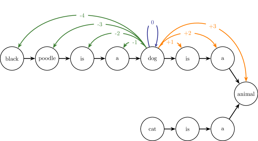
(a) Relative positions $P$ for dog in $\ell$GLM

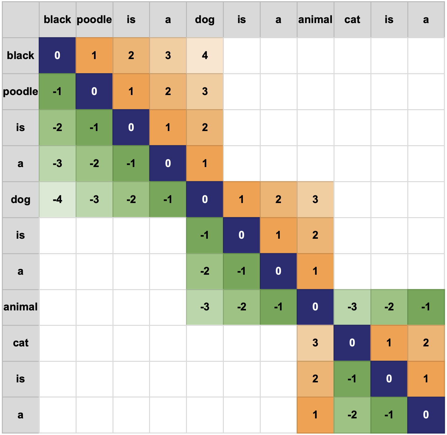
(b) Relative position matrix $P$ for $\ell$GLM

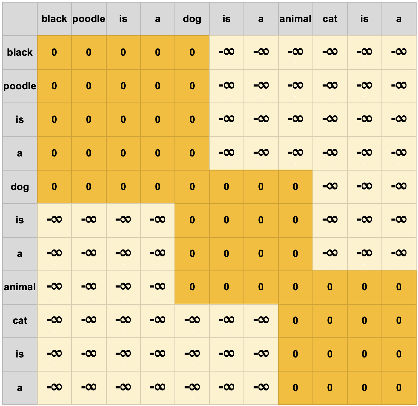
(c) Mask $M$ for $\ell$GLM

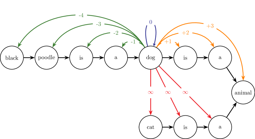
(d) Relative position $P$ for dog in $g$GLM

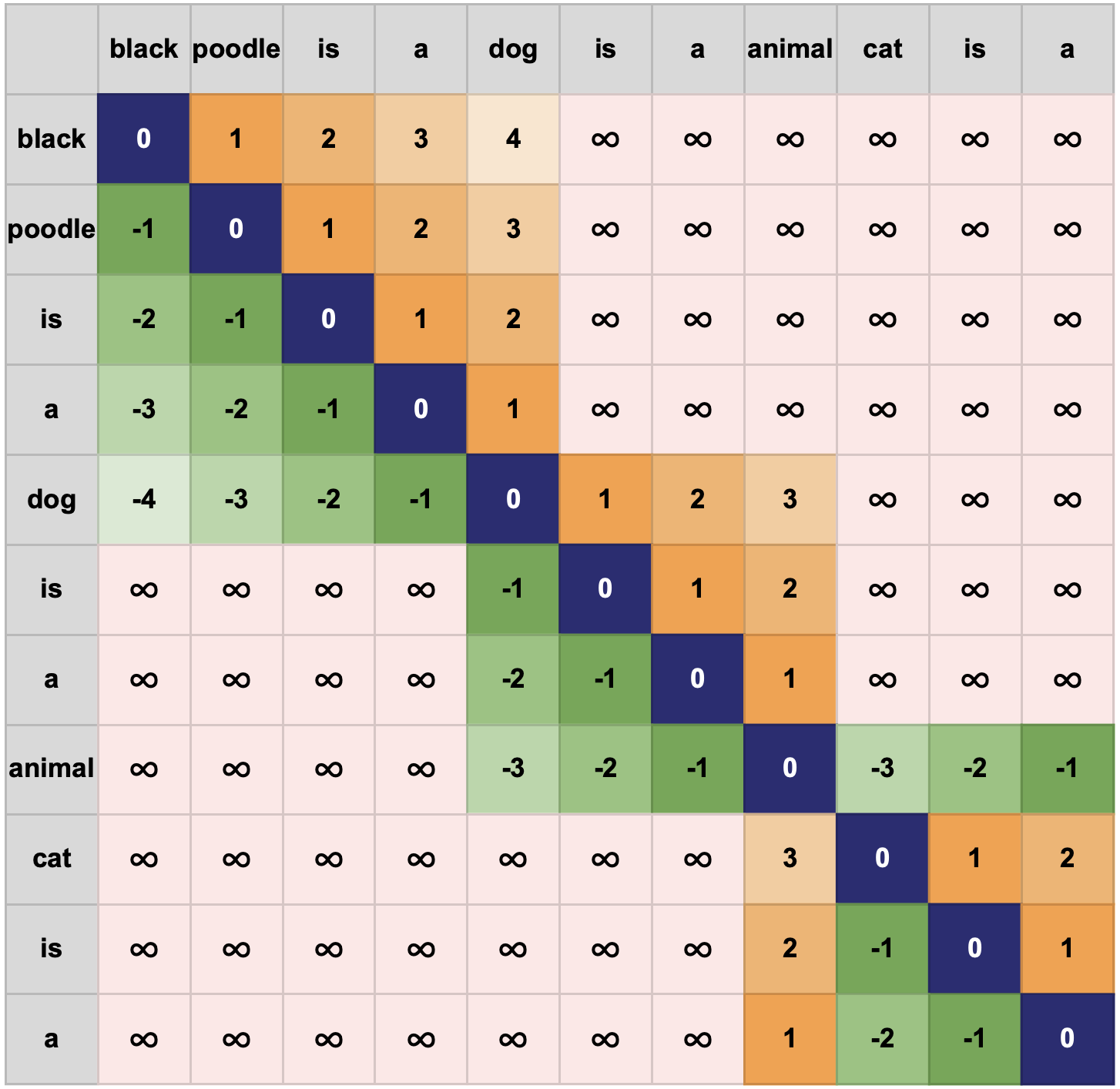
(e) Relative position matrix $P$ for $g$GLM

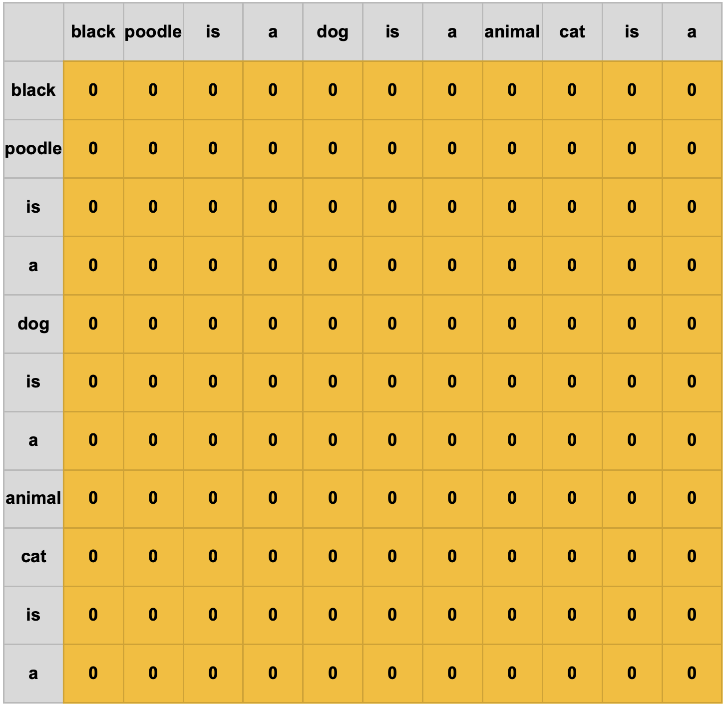
(f) Mask $M$ for $g$GLM

Figure 4: Relative positions $P$ and masking $M$ for $\ell$GLM and $g$GLM.

	Relation	Verbalization
Used as relation label	Antonym	is an antonym of
	AtLocation	is in
	CapableOf	is capable of
	Causes	causes
	CausesDesire	causes desire
	DistinctFrom	is distinct from
	FormOf	is a form of
	HasContext	has context
	HasPrerequisite	has prerequisite
	HasProperty	is
	HasSubevent	has subevent
	IsA	is a
	MannerOf	is a manner of
	MotivatedByGoal	is motivated by
	PartOf	is a part of
	Synonym	is a synonym of
	UsedFor	is used for
Not used as relation label	CreatedBy	is created by
	DefinedAs	is defined as
	Desires	desires
	Entails	entails
	HasA	has
	HasFirstSubevent	starts with
	HasLastSubevent	ends with
	InstanceOf	is an instance of
	LocatedNear	is near
	MadeOf	is made of
	NotCapableOf	is not capable of
	NotDesires	does not desire
	NotHasProperty	is not
	ReceivesAction	receives action
	RelatedTo	is related to
	SymbolOf	is a symbol of

Table 4: Verbalization templates for relations in ConceptNet. The upper part of the relations are the 17 classes in the classification task.

	Parameter	Value
GLM, LM & GT	Loss	cross entropy loss
	Optimizer	AdamW
	Learning rate	$110-4\text{\,}$ (FT) & $510-3\text{\,}$ (LP)
	Batchsize	32
	Max. # epochs	50
	Early stopping criterion	dev loss
	Early stopping # epochs	5
	# parameters in small	35B (FT) & 8k (LP)
	# parameters in base	110B (FT) & 13k (LP)
	# parameters in large	335B (FT) & 17k (LP)
GNN	Loss	cross entropy loss
	Optimizer	AdamW
	Learning rate	$510-3\text{\,}$
	Batchsize	32
	Max. # epochs	50
	Early stopping criterion	dev loss
	Early stopping # epochs	5
	# layers	3
	hidden channel dimension	64
	non-linearity	ReLU

Table 5: Hyperparameters. FT stands for finetuning and LP stand for linear probing. “# parameters” is the number of traininable parameters.

References

- Alon and Yahav (2021) Uri Alon and Eran Yahav. 2021. On the bottleneck of graph neural networks and its practical implications. In International Conference on Learning Representations.
- Auer et al. (2007) Sören Auer, Christian Bizer, Georgi Kobilarov, Jens Lehmann, Richard Cyganiak, and Zachary Ives. 2007. Dbpedia: A nucleus for a web of open data. In The Semantic Web, pages 722–735, Berlin, Heidelberg. Springer Berlin Heidelberg.
- Banarescu et al. (2013) Laura Banarescu, Claire Bonial, Shu Cai, Madalina Georgescu, Kira Griffitt, Ulf Hermjakob, Kevin Knight, Philipp Koehn, Martha Palmer, and Nathan Schneider. 2013. Abstract Meaning Representation for sembanking. In Proceedings of the 7th Linguistic Annotation Workshop and Interoperability with Discourse, pages 178–186, Sofia, Bulgaria. Association for Computational Linguistics.
- Bosselut et al. (2019) Antoine Bosselut, Hannah Rashkin, Maarten Sap, Chaitanya Malaviya, Asli Celikyilmaz, and Yejin Choi. 2019. COMET: Commonsense transformers for automatic knowledge graph construction. In Proceedings of the 57th Annual Meeting of the Association for Computational Linguistics, pages 4762–4779, Florence, Italy. Association for Computational Linguistics.
- Bronstein et al. (2021) Michael M Bronstein, Joan Bruna, Taco Cohen, and Petar Veličković. 2021. Geometric deep learning: Grids, groups, graphs, geodesics, and gauges. arXiv preprint arXiv:2104.13478.
- Chen et al. (2020) Deli Chen, Yankai Lin, Wei Li, Peng Li, Jie Zhou, and Xu Sun. 2020. Measuring and relieving the over-smoothing problem for graph neural networks from the topological view. Proceedings of the AAAI Conference on Artificial Intelligence, 34(04):3438–3445.
- Dufter et al. (2022) Philipp Dufter, Martin Schmitt, and Hinrich Schütze. 2022. Position information in transformers: An overview. Computational Linguistics, 48(3):733–763.
- Galkin et al. (2023) Mikhail Galkin, Xinyu Yuan, Hesham Mostafa, Jian Tang, and Zhaocheng Zhu. 2023. Towards foundation models for knowledge graph reasoning. arXiv preprint.
- Gardent et al. (2017) Claire Gardent, Anastasia Shimorina, Shashi Narayan, and Laura Perez-Beltrachini. 2017. The WebNLG challenge: Generating text from RDF data. In Proceedings of the 10th International Conference on Natural Language Generation, pages 124–133, Santiago de Compostela, Spain. Association for Computational Linguistics.
- Gehring et al. (2017) Jonas Gehring, Michael Auli, David Grangier, and Yann Dauphin. 2017. A convolutional encoder model for neural machine translation. In Proceedings of the 55th Annual Meeting of the Association for Computational Linguistics (Volume 1: Long Papers), pages 123–135, Vancouver, Canada. Association for Computational Linguistics.
- Huguet Cabot and Navigli (2021) Pere-Lluís Huguet Cabot and Roberto Navigli. 2021. REBEL: Relation extraction by end-to-end language generation. In Findings of the Association for Computational Linguistics: EMNLP 2021, pages 2370–2381, Punta Cana, Dominican Republic. Association for Computational Linguistics.
- Hwang et al. (2021) Jena D. Hwang, Chandra Bhagavatula, Ronan Le Bras, Jeff Da, Keisuke Sakaguchi, Antoine Bosselut, and Yejin Choi. 2021. Comet-atomic 2020: On symbolic and neural commonsense knowledge graphs. In AAAI.
- Ke et al. (2021) Guolin Ke, Di He, and Tie-Yan Liu. 2021. Rethinking positional encoding in language pre-training. In International Conference on Learning Representations.
- Kipf and Welling (2017) Thomas N. Kipf and Max Welling. 2017. Semi-supervised classification with graph convolutional networks. In International Conference on Learning Representations (ICLR).
- Koncel-Kedziorski et al. (2019) Rik Koncel-Kedziorski, Dhanush Bekal, Yi Luan, Mirella Lapata, and Hannaneh Hajishirzi. 2019. Text Generation from Knowledge Graphs with Graph Transformers. In Proceedings of the 2019 Conference of the North American Chapter of the Association for Computational Linguistics: Human Language Technologies, Volume 1 (Long and Short Papers), pages 2284–2293, Minneapolis, Minnesota. Association for Computational Linguistics.
- Li et al. (2021) Junyi Li, Tianyi Tang, Wayne Xin Zhao, Zhicheng Wei, Nicholas Jing Yuan, and Ji-Rong Wen. 2021. Few-shot Knowledge Graph-to-Text Generation with Pretrained Language Models. In ACL Findings.
- Lin et al. (2019) Bill Yuchen Lin, Xinyue Chen, Jamin Chen, and Xiang Ren. 2019. KagNet: Knowledge-aware graph networks for commonsense reasoning. In Proceedings of the 2019 Conference on Empirical Methods in Natural Language Processing and the 9th International Joint Conference on Natural Language Processing (EMNLP-IJCNLP), pages 2829–2839, Hong Kong, China. Association for Computational Linguistics.
- Malaviya et al. (2020) Chaitanya Malaviya, Chandra Bhagavatula, Antoine Bosselut, and Yejin Choi. 2020. Commonsense knowledge base completion with structural and semantic context. Proceedings of the 34th AAAI Conference on Artificial Intelligence.
- Min et al. (2022) Erxue Min, Runfa Chen, Yatao Bian, Tingyang Xu, Kangfei Zhao, Wen bing Huang, Peilin Zhao, Junzhou Huang, Sophia Ananiadou, and Yu Rong. 2022. Transformer for graphs: An overview from architecture perspective. ArXiv, abs/2202.08455.
- Müller et al. (2023) Luis Müller, Christopher Morris, Mikhail Galkin, and Ladislav Rampášek. 2023. Attending to Graph Transformers. Arxiv preprint.
- Pan et al. (2024) Shirui Pan, Linhao Luo, Yufei Wang, Chen Chen, Jiapu Wang, and Xindong Wu. 2024. Unifying large language models and knowledge graphs: A roadmap. IEEE Transactions on Knowledge and Data Engineering (TKDE).
- Plenz et al. (2023) Moritz Plenz, Juri Opitz, Philipp Heinisch, Philipp Cimiano, and Anette Frank. 2023. Similarity-weighted construction of contextualized commonsense knowledge graphs for knowledge-intense argumentation tasks. In Proceedings of the 61st Annual Meeting of the Association for Computational Linguistics (Volume 1: Long Papers), pages 6130–6158, Toronto, Canada. Association for Computational Linguistics.
- Press et al. (2022) Ofir Press, Noah Smith, and Mike Lewis. 2022. Train short, test long: Attention with linear biases enables input length extrapolation. In International Conference on Learning Representations.
- Raffel et al. (2020) Colin Raffel, Noam Shazeer, Adam Roberts, Katherine Lee, Sharan Narang, Michael Matena, Yanqi Zhou, Wei Li, and Peter J. Liu. 2020. Exploring the limits of transfer learning with a unified text-to-text transformer. Journal of Machine Learning Research, 21(140):1–67.
- Ribeiro et al. (2021) Leonardo F. R. Ribeiro, Martin Schmitt, Hinrich Schütze, and Iryna Gurevych. 2021. Investigating pretrained language models for graph-to-text generation. In Proceedings of the 3rd Workshop on Natural Language Processing for Conversational AI, pages 211–227, Online. Association for Computational Linguistics.
- Ribeiro et al. (2020) Leonardo F. R. Ribeiro, Yue Zhang, Claire Gardent, and Iryna Gurevych. 2020. Modeling global and local node contexts for text generation from knowledge graphs. Transactions of the Association for Computational Linguistics, 8:589–604.
- Ruoss et al. (2023) Anian Ruoss, Grégoire Delétang, Tim Genewein, Jordi Grau-Moya, Róbert Csordás, Mehdi Bennani, Shane Legg, and Joel Veness. 2023. Randomized positional encodings boost length generalization of transformers. In Proceedings of the 61st Annual Meeting of the Association for Computational Linguistics (Volume 2: Short Papers), pages 1889–1903, Toronto, Canada. Association for Computational Linguistics.
- Schmitt et al. (2021) Martin Schmitt, Leonardo F. R. Ribeiro, Philipp Dufter, Iryna Gurevych, and Hinrich Schütze. 2021. Modeling graph structure via relative position for text generation from knowledge graphs. In Proceedings of the Fifteenth Workshop on Graph-Based Methods for Natural Language Processing (TextGraphs-15), pages 10–21, Mexico City, Mexico. Association for Computational Linguistics.
- Schmitt et al. (2020) Martin Schmitt, Sahand Sharifzadeh, Volker Tresp, and Hinrich Schütze. 2020. An unsupervised joint system for text generation from knowledge graphs and semantic parsing. In Proceedings of the 2020 Conference on Empirical Methods in Natural Language Processing (EMNLP), pages 7117–7130, Online. Association for Computational Linguistics.
- Shaw et al. (2018) Peter Shaw, Jakob Uszkoreit, and Ashish Vaswani. 2018. Self-attention with relative position representations. In Proceedings of the 2018 Conference of the North American Chapter of the Association for Computational Linguistics: Human Language Technologies, Volume 2 (Short Papers), pages 464–468, New Orleans, Louisiana. Association for Computational Linguistics.
- Speer et al. (2017) Robyn Speer, Joshua Chin, and Catherine Havasi. 2017. Conceptnet 5.5: An open multilingual graph of general knowledge. In Proceedings of the Thirty-First AAAI Conference on Artificial Intelligence, AAAI’17, page 4444–4451. AAAI Press.
- Su et al. (2021) Jianlin Su, Yu Lu, Shengfeng Pan, Bo Wen, and Yunfeng Liu. 2021. Roformer: Enhanced transformer with rotary position embedding. CoRR, abs/2104.09864.
- Vaswani et al. (2017) Ashish Vaswani, Noam Shazeer, Niki Parmar, Jakob Uszkoreit, Llion Jones, Aidan N Gomez, Ł ukasz Kaiser, and Illia Polosukhin. 2017. Attention is all you need. In Advances in Neural Information Processing Systems, volume 30. Curran Associates, Inc.
- Veličković et al. (2018) Petar Veličković, Guillem Cucurull, Arantxa Casanova, Adriana Romero, Pietro Liò, and Yoshua Bengio. 2018. Graph Attention Networks. International Conference on Learning Representations.
- Wang et al. (2020a) Peifeng Wang, Nanyun Peng, Filip Ilievski, Pedro Szekely, and Xiang Ren. 2020a. Connecting the dots: A knowledgeable path generator for commonsense question answering. In Findings of the Association for Computational Linguistics: EMNLP 2020, pages 4129–4140, Online. Association for Computational Linguistics.
- Wang et al. (2021) Ruize Wang, Duyu Tang, Nan Duan, Zhongyu Wei, Xuanjing Huang, Jianshu Ji, Guihong Cao, Daxin Jiang, and Ming Zhou. 2021. K-Adapter: Infusing Knowledge into Pre-Trained Models with Adapters. In Findings of the Association for Computational Linguistics: ACL-IJCNLP 2021, pages 1405–1418, Online. Association for Computational Linguistics.
- Wang et al. (2020b) Tianming Wang, Xiaojun Wan, and Hanqi Jin. 2020b. AMR-to-text generation with graph transformer. Transactions of the Association for Computational Linguistics, 8:19–33.
- West et al. (2023) Peter West, Ronan Bras, Taylor Sorensen, Bill Lin, Liwei Jiang, Ximing Lu, Khyathi Chandu, Jack Hessel, Ashutosh Baheti, Chandra Bhagavatula, and Yejin Choi. 2023. NovaCOMET: Open commonsense foundation models with symbolic knowledge distillation. In Findings of the Association for Computational Linguistics: EMNLP 2023, pages 1127–1149, Singapore. Association for Computational Linguistics.
- Yu et al. (2022) Wenhao Yu, Chenguang Zhu, Yuwei Fang, Donghan Yu, Shuohang Wang, Yichong Xu, Michael Zeng, and Meng Jiang. 2022. Dict-BERT: Enhancing language model pre-training with dictionary. In Findings of the Association for Computational Linguistics: ACL 2022, pages 1907–1918, Dublin, Ireland. Association for Computational Linguistics.
- Zhao et al. (2023) Jianan Zhao, Meng Qu, Chaozhuo Li, Hao Yan, Qian Liu, Rui Li, Xing Xie, and Jian Tang. 2023. Learning on large-scale text-attributed graphs via variational inference. In The Eleventh International Conference on Learning Representations.