When Does Feature Learning Happen?
Perspective from an Analytically Solvable Model

Abstract

We identify and solve a hidden-layer model that is analytically tractable at any finite width and whose limits exhibit both the kernel phase and the feature learning phase. We analyze the phase diagram of this model in all possible limits of common hyperparameters including width, layer-wise learning rates, scale of output, and scale of initialization. We apply our result to analyze how and when feature learning happens in both infinite and finite-width models. Three prototype mechanisms of feature learning are identified: (1) learning by alignment, (2) learning by disalignment, and (3) learning by rescaling. In sharp contrast, neither of these mechanisms is present when the model is in the kernel regime. This discovery explains why large initialization often leads to worse performance. Lastly, we empirically demonstrate that discoveries we made for this analytical model also appear in nonlinear networks in real tasks.

1 Introduction

Let $f_{\theta}(x)\in\mathbb{R}$ be our neural network under consideration. It has been shown that for a neural network under certain types of scaling towards infinite size (or certain parameters), the learning dynamics can be precisely described by the NTK dynamics (Jacot et al.,, 2018). For the MSE loss function, the dynamics are shown to be linear in the kernel regime: $\dot{f}(x)=-\mathbb{E}_{x^{\prime}}[K(x,x^{\prime})(f(x^{\prime})-y(x^{\prime}))]$, where $\mathbb{E}_{x^{\prime}}$ denotes averaging over the training set and

$$K(x,x^{\prime})=\nabla_{\theta}f(x)\cdot\nabla_{\theta}f(x^{\prime})$$ (1)

is the neural tangent kernel (NTK) and does not change throughout training. We say that a model in the kernel regime if the NTK of the model remains unchanged throughout training. Additionally, Chizat et al., (2018) showed that if the network is initialized in a special way, any model is in the kernel regime under a certain scaling of hyperparameters other than the width. In other words, the kernel regime is not a special feature of infinite-width networks and can also emerge naturally in finite-size models. Afterward, it has been shown that if one scales the neural network towards infinity under different learning rates and output multiplier scaling, the network can be described by the feature learning regime, where the NTK does change significantly throughout training (Yang and Hu,, 2020). Due to the paramount importance of the NTK in understanding the training and generalization of neural networks, a lot of works are devoted to understanding the structure of $K$ and how it changes as training proceeds (Hanin and Nica,, 2019; Liu et al.,, 2020; Huang et al.,, 2020; Huang and Yau,, 2020; Chen et al.,, 2020; Baratin et al.,, 2021; Atanasov et al.,, 2021; Geiger et al.,, 2021; Bordelon and Pehlevan,, 2022; Radhakrishnan et al.,, 2022; Simon et al.,, 2023). Ideally, we want a theory that allows us to precisely characterize the dynamics of NTK and whether the current model under training is in the kernel phase or the feature learning regime.

However, despite the progress in understanding these infinite-size models, there has been very limited result in understanding how feature learning actually happens and the relationship between these two limiting regimes. Arguably, the main theoretical gap is that until now, we do not know a single example of a finite-size analytically tractable model, whose NTK dynamics can be analytically and precisely described and exhibits both the NTK and feature learning regimes under different scalings. Having such a model would help us both understand how the insights we have extensively derived for infinite-size models carry over to finite-size models and also how feature learning happens in an infinite-size model.

The foremost contribution of this work is to analytically solve the evolution dynamics of the NTK of a minimal finite-size model for an arbitrary choice of hyperparameters and initialization. The minimal model we will solve is a one-hidden-layer linear network. While the model is simple in nature, its loss landscape is nonconvex and its training involves strongly coupled dynamics, and the exact solution of its learning dynamics is not yet known. A result highly relevant to ours is that of Saxe et al., (2013), where the exact solution of linear nets under the orthogonal initialization (Arpit et al.,, 2019; Hu et al.,, 2020) is found. More recently, Atanasov et al., (2021) utilized the result to understand the evolution of the NTK starting from a small initialization. However, the limitation of the solution in Saxe et al., (2013) is clear – under the orthogonal initialization, the model is necessarily in the feature learning phase, and one cannot understand the causal reasons for the NTK to change.

2 An Exactly Solvable Model

In this section, we first present the solution of the learning dynamics. We then analyze the dynamics closely to show that there are three major mechanisms of feature learning: (1) alignment, (2) disalignment, and (3) rescaling. All the proofs are presented in Section A. All experimental details for reproducing the experiments are given in Section B.

2.1 Solution

Let us consider a two-layer linear network trained on the MSE loss. The loss function is

$$\tilde{L}=\mathbb{E}_{\tilde{x}}\left[\left(\gamma\sum_{i=1}^{d}\sum_{j=1}^{d_{0}}u_{i}w_{ij}\tilde{x}_{j}-y(\tilde{x})\right)^{2}\right],$$ (2)

where we have treated $y$ as a function of $\tilde{x}$ and $\mathbb{E}_{\tilde{x}}$ denotes the averaging over the training set. We restrict to the case where all the data points lie on a one-dimensional subspace. Namely, we have that with probability $1$, $\tilde{x}=an$ for a random variable $a\in\mathbb{R}$ and a constant unit vector $n$.

Then, the loss becomes

$$\tilde{L}=(\mathbb{E}_{a}[a^{2}])\left(\gamma\sum_{i=1}^{d}\sum_{j=1}^{d_{0}}u_{i}w_{ij}n_{j}\right)^{2}-2(\mathbb{E}_{a}[ay(an)])\left(\gamma\sum_{i=1}^{d}\sum_{j=1}^{d_{0}}u_{i}w_{ij}n_{j}\right)+\mathbb{E}_{\tilde{x}}[y(\tilde{x})^{2}],$$ (3)

Despite the simplicity of this problem, its solution has not been analytically analyzed. Only in two special settings the dynamics of GD has been solved for this problem. One is the standard kernel regime, where the dynamics are exactly linear (Jacot et al.,, 2018); the second case is when the two layers are initialized to be perfectly aligned, where $u$ is a left eigenvector of $w$ (Saxe et al.,, 2013).

Without loss of generality, this setting is equivalent to the case when $\tilde{x}$ is only a single data point

$$L=\left(\gamma\sum_{i=1}^{d}\sum_{j=1}^{d_{0}}u_{i}w_{ij}x_{j}-y\right)^{2},$$ (4)

where $x=\sqrt{\mathbb{E}_{a}[a^{2}]}n$ and $y=\frac{\mathbb{E}_{a}[ay(an)]}{\sqrt{\mathbb{E}_{a}[a^{2}]}}$. From now on, we will consider (4) for notational simplicity.

A little more general than the conventional study of NTK, the problem setting we consider is where two different layers are trained with different learning rates, which is sometimes used in practice in training neural networks (Liu et al.,, 2022):

$$\frac{du_{i}}{dt}=-\eta_{u}\frac{\partial L}{\partial u_{i}},$$ (5)

$$\frac{dw_{i}}{dt}=-\eta_{w}\frac{\partial L}{\partial w_{ij}},$$

where the learning rates of two layers are $\eta_{u}$ and $\eta_{w}$, respectively. The following theorem gives a precise characterization of the dynamics of $u_{i}$ and $w_{i}$ for an arbitrary initialization and hyperparameter choice.

Theorem 1.

Let

$$p_{i}(t):=\frac{1}{2\rho}(\sqrt{\eta_{u}}\sum_{j=1}^{d_{0}}w_{ij}(t)x_{j}+\sqrt{\eta_{w}}\rho u_{i}(t)),\ q_{i}(t):=\frac{1}{2\rho}(\sqrt{\eta_{u}}\sum_{j=1}^{d_{0}}w_{ij}(t)x_{j}-\sqrt{\eta_{w}}\rho u_{i}(t))$$ (6)

and

$$P:=\frac{1}{d}\sum_{j=1}^{d}p_{j}(0)^{2},\ Q:=\frac{1}{d}\sum_{j=1}^{d}q_{j}(0)^{2},$$ (7)

where $\rho:=\sqrt{\frac{1}{d_{0}}\sum_{i=0}^{d_{0}}x_{i}^{2}}$. Assuming $P\neq 0$, then

$$p_{i}(t)=p_{i}(0)\left[\frac{\alpha_{+}+\xi(t)\alpha_{-}}{1-\xi(t)}\right]^{1/2},$$ (8)

$$q_{i}(t)=q_{i}(0)\left[\frac{\alpha_{+}+\xi(t)\alpha_{-}}{1-\xi(t)}\right]^{-1/2},$$ (9)

where

$$\xi(t):=\frac{1-\alpha_{+}}{1+\alpha_{-}}\exp\left(-4t/t_{c}\right),$$ (10)

$$t_{c}:=1/\left(\sqrt{\eta_{u}\eta_{w}\gamma^{2}\rho^{2}y^{2}+4\rho^{4}(\gamma^{2}d)^{2}PQ}\right),$$ (11)

$$\alpha_{\pm}:=\frac{1}{2(\gamma^{2}d)\rho^{2}P}\left(\sqrt{\eta_{u}\eta_{w}}\gamma\rho y\pm\sqrt{\eta_{u}\eta_{w}\gamma^{2}\rho^{2}y^{2}+4\rho^{4}(\gamma^{2}d)^{2}PQ}\right).$$ (12)

We refer to Proposition 1 in Appendix A for the special case $P=0$.

Let us first analyze each term and clarify their meanings. In the theorem, we have transformed $u_{i}$ and $w_{ij}$ into an alternative basis $p_{i}$ and $q_{i}$, and $\xi=\xi(t)$ is the only term that is time-dependent. Note that $\xi$ decays exponentially towards zero at the time scale $t_{c}$.

By definition, we have that

$$u_{i}(t)=\frac{1}{\sqrt{\eta_{w}}}(p_{i}(t)-q_{i}(t)),$$ (13)

and

$$w_{ij}(t)=w_{ij}(0)+\left(p_{i}(t)-p_{i}(0)+q_{i}(t)-q_{i}(0)\right)\frac{x_{j}}{\sqrt{\eta_{u}}\rho}.$$ (14)

The constants $\alpha_{+}\alpha_{-}=\frac{Q}{P}$ are two asymptotic scale factors. In the limit $t\to\infty$, we have that

$$p_{i}(\infty)=p_{i}(0)\sqrt{\alpha_{+}},$$ (15)

$$q_{i}(\infty)=q_{i}(0)/\sqrt{\alpha_{+}}.$$ (16)

This directly gives us the mapping between the initialization to the converged solution. Unlike a strongly convex problem where the solution is independent of the initialization, we see that the converged solution for our model is strongly dependent on the initialization and on the choice of hyperparameter. Perhaps surprisingly, because $\alpha_{\pm}$ are functions of the learning rates, the converged solution also depends directly on the magnitudes of the learning rates. This directly tells us the implicit bias of gradient-descent training for this problem. Another special feature of the solution is that for any direction orthogonal to $x$, the model will remain unchanged during training. Let $m\perp x$, we have that $\sum_{j}w_{ij}(t)m_{j}=\sum_{j}w_{ij}(0)m_{j}$. Namely, the output of the model in the subspace where there is no data remains constant during training.

In the theorem, what is especially important is the characteristic time scale $t_{c}$, which is roughly the time it takes for learning to happen. Notably, the squared learning speed $t_{c}^{-2}$ depends on two competing factors:

$$t_{c}^{-2}=\underbrace{\eta_{u}\eta_{w}\gamma^{2}\rho^{2}y^{2}}_{\text{contribution from feature learning}}+\underbrace{4\rho^{4}(\gamma^{2}d)^{2}PQ}_{\text{contribution from kernel learning}}$$ (17)

The first factor depends on the input-output correlation and learning rate, and we will see that this term is a sign of feature learning. The second term depends only on the input data and on the model initialization. We will see that when this term is dominant, the model is in the kernel regime. In fact, this result already calls for a strong interpretation: the learning of the kernel regime is driven by the initialization and the input feature, and the learning in the feature learning regime is driven by the target mapping and large learning rates.

Another pair of important quantities are $P$ and $Q$, which are essentially the initialization of the model. For $\eta_{u}=\eta_{w}$, a small $P$ implies that $w_{i}(0)\approx-u_{i}(0)$ for all $i$, which implies that the model is close to anti-parallel at the start of training. Likewise, a small $Q$ implies that $w_{i}(0)\approx u_{i}(0)$ for all $i$; namely, the two layers start training when they are approximately parallel. When both $P$ and $Q$ are small, the model is initialized close to the origin, which is a saddle point. We will also see below that in the kernel regime, we always have $Q=P$.

With this theorem, one can identify the following quantities of interest to us. First, we note that when different learning rates are used for different layers, the NTK needs to be defined slightly differently from the conventional definition. For the MSE loss, the NTK is the quantity $K$ that enters the following dynamics: $\frac{df(x)}{dt}=2K(x,x^{\prime})(f(x^{\prime})-y)$, which implies that for our problem,

$$K(x,x^{\prime})=\gamma^{2}x^{T}(\eta_{w}W^{T}W+\eta_{u}||u||^{2}I)x^{\prime},$$ (18)

Note that when $\eta_{w}=\eta_{u}$, this definition agrees with the common definition of NTK.

The model $f(x)=\gamma\sum_{i=1}^{d}\sum_{j=1}^{d_{0}}u_{i}w_{ij}x_{j}$ is

$$f(x)=\frac{\gamma d}{\sqrt{\eta_{u}\eta_{w}}}\left(P\frac{\alpha_{+}+\xi\alpha_{-}}{1-\xi}-Q\frac{1-\xi}{\alpha_{+}+\xi\alpha_{-}}\right).$$ (19)

which implies that $\lim_{t\to\infty}f(x)=\frac{\gamma d}{\sqrt{\eta_{u}\eta_{w}}}(\alpha_{+}P-Q/\alpha_{+})=y$ for $P\neq 0$.

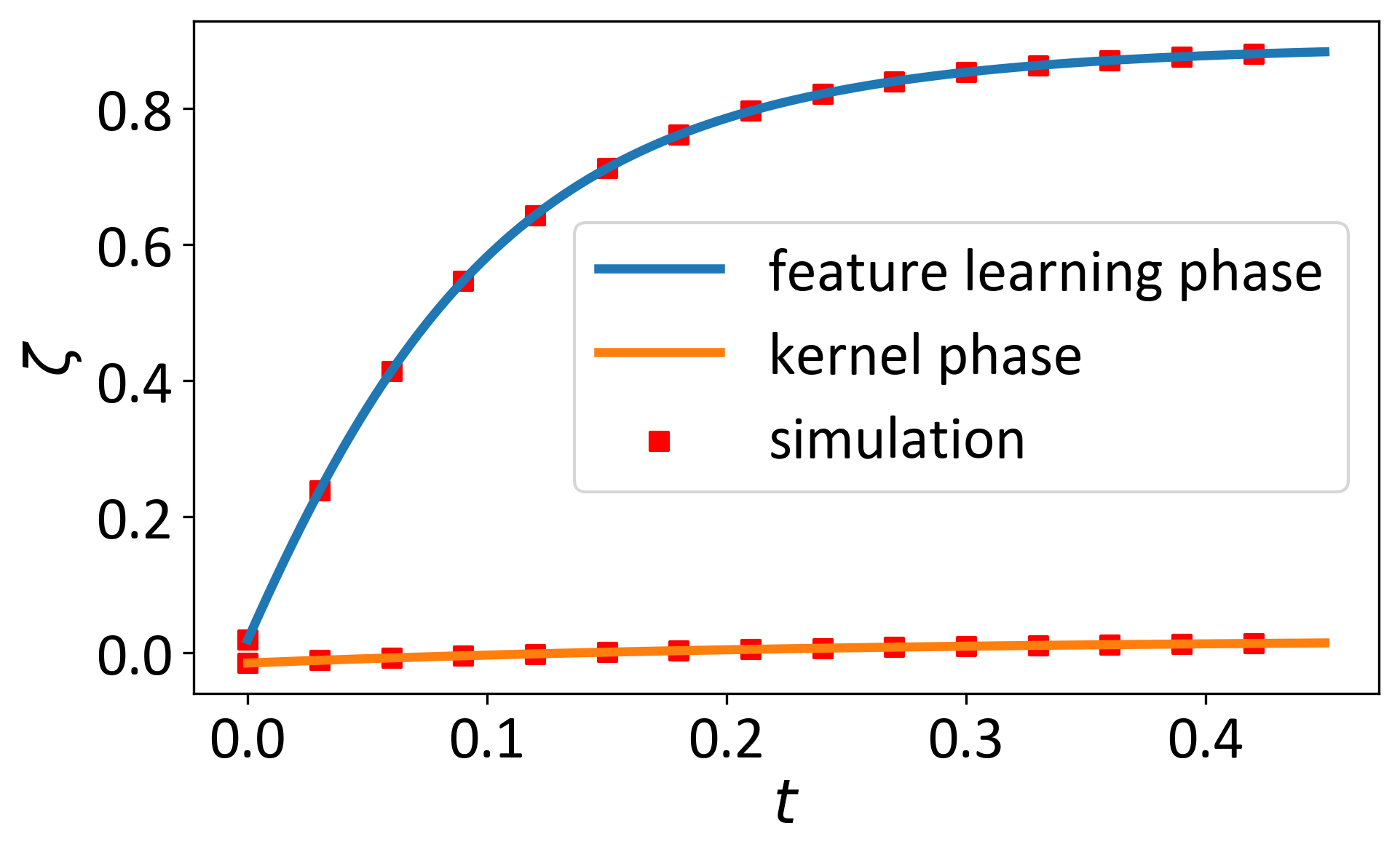
(a) alignment in linear network

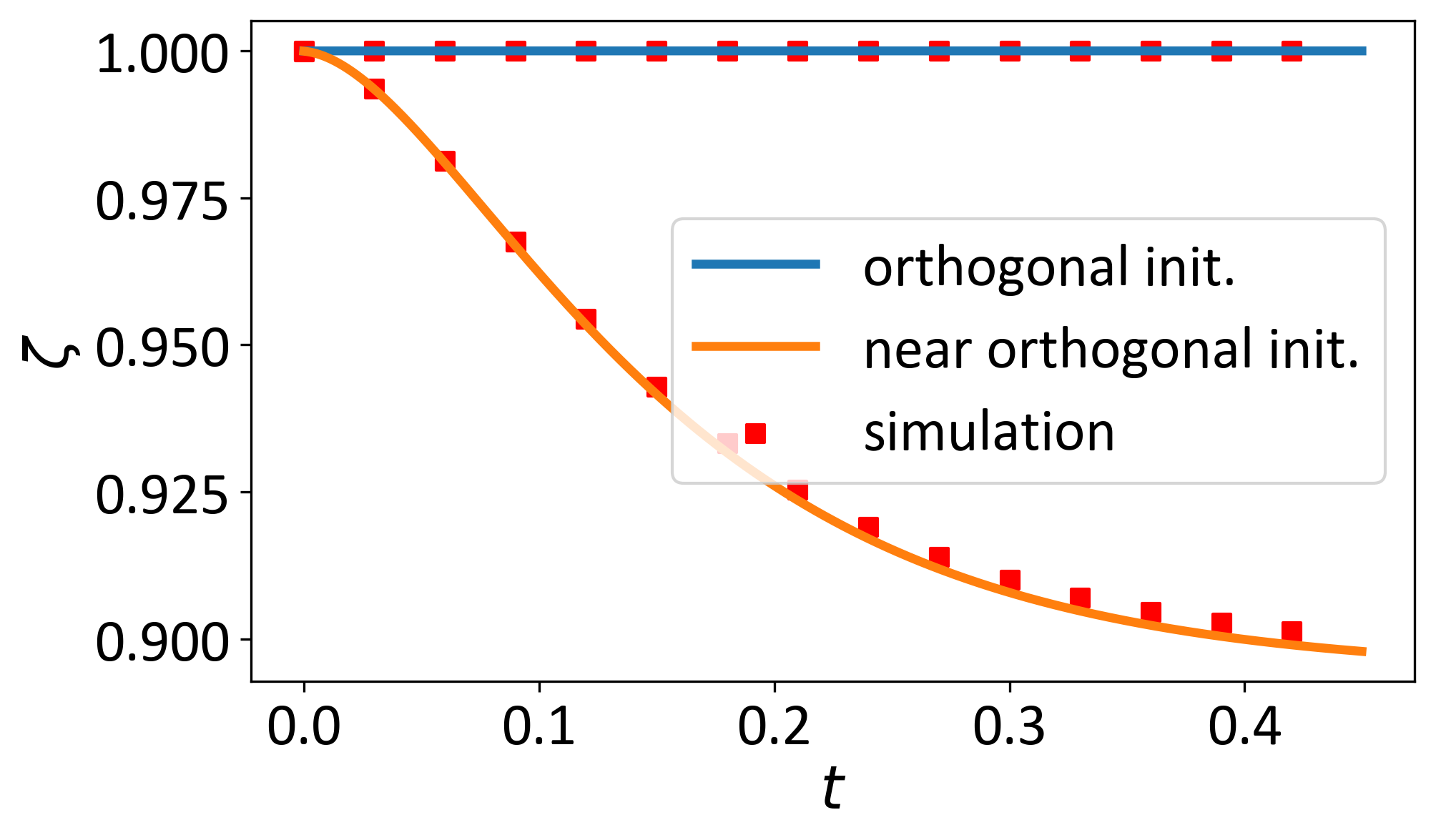
(b) disalignment in linear network

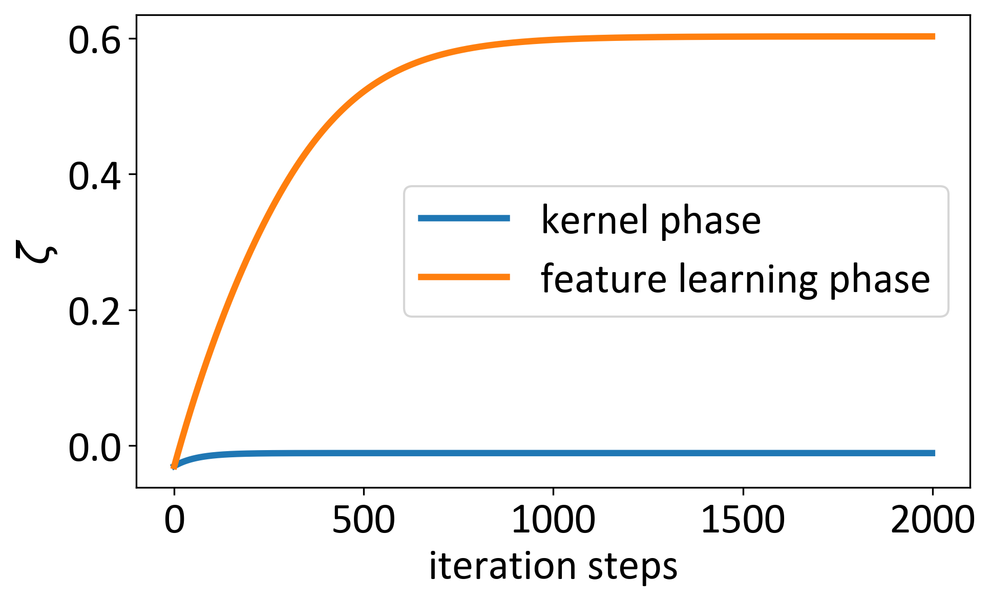
(c) alignment in ReLU network

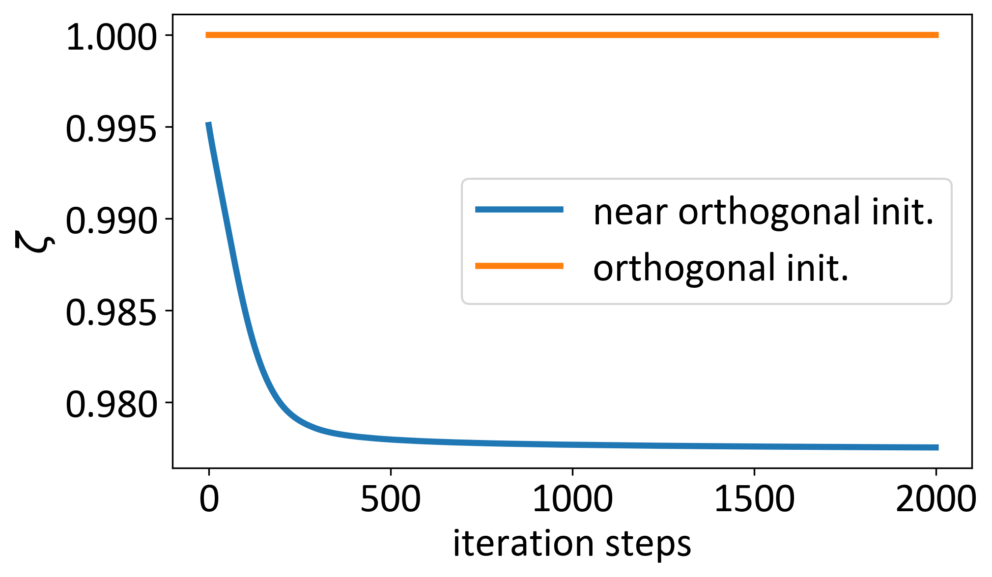
(d) disalignment in ReLU network

Figure 1: The evolution of the alignment angle $\zeta$ between $u$ and $v$ on a two-layer linear and ReLU network with $d=10000$. When the initialization scale is large, the model learns by disalignment; when the initialization scale is small, the model learns by alignment. Also, see Section B for additional experiments with adaptive gradients.

2.2 Learning by Alignment and Disalignment

Before we discuss the various phase diagrams implied by Theorem 1, we first focus on a crucial effect predicted by this theorem, which differentiates it from previous results on similar problems. An important quantity our theory enables us to study is the evolution of the layer alignment $\zeta$:

$$\zeta(t):=\frac{u^{T}w}{||u||||w||}$$ (20)

which is the cosine similarity between $u$ and $w$. Here, we have assumed that $x$ is one-dimensional, which is without loss of generality by Theorem 1 because the dynamics of GD training has only a rank-1 effect on the model. This quantity is especially interesting to study because it tells us how well-aligned the two layers are during training. Notably, this quantity is always zero if and only if the model is in the kernel regime, so it is also a great metric to probe how feature learning happens.

Assuming that $x=1$ and denoting $\alpha(t)=\frac{\alpha_{+}+\xi\alpha_{-}}{1-\xi}$, we have by Theorem 1:

$$\zeta(t)=\frac{\alpha(t)P-Q/\alpha(t)}{\sqrt{(\alpha(t)P+Q/\alpha(t))^{2}-(\frac{2}{d}\sum p_{i}q_{i})^{2}}},$$ (21)

Note that $4p_{i}q_{i}=u_{i}^{2}-w_{i}^{2}=const$ does not change during training. In general, the angle evolves by an $O(1)$ amount during training. In fact, the angle remains unchanged only in the orthogonal initialization case, or in the kernel phase where $\alpha(t)\approx 1$.

Let us first consider the kernel case. Here, the easiest way to see that $\zeta$ remains zero is to note that in the kernel regime, $\|u\|$ and $\|w\|$ are of order $\sqrt{d}$, whereas $u^{T}w$ is always of order $1/\gamma$. Therefore, $\zeta(t)=o(1)$ in the NTK phase (see Section 3) and vanishes in the limit $d\to\infty$. Alternatively, one can see this from Theorem 1, which implies that in the kernel regime $\alpha(t)=1$ is a constant, which in turn implies that $\zeta(t)=0$. Therefore, in the kernel regime, the two layers are essentially orthogonal to each other throughout training. This points to one reason why the kernel phase tends to have poorer performance. For a data point $x$, the hidden representation is $wx$, but predominantly many information in $wx$ is ignored after the the layer $u$. This implies that the model will have a disproportionately larger norm than what is actually required to fit the data, which could in turn imply strong overfitting.

The second case that prior literature has analyzed is when the two layers are initialized in a parallel way (Saxe et al.,, 2013). This setting is often called the “orthogonal initialization.” In the orthogonal initialization, $u$ is parallel to $w$, and so $p_{i}=Cq_{i}$. In this case, we can verify that

$$\zeta(t)^{2}=\frac{(\alpha(t)C-1/\alpha(t))^{2}}{(\alpha(t)C+1/\alpha(t))^{2}-4C^{2}}=1,$$ (22)

meaning that $u$ and $w$ remain parallel or anti-parallel throughout training. Therefore, prior literature offers no clue regarding how $\zeta$ evolves in general.

Our solution implies a rather remarkable fact: $\zeta$ is always a monotonic function of $t$. To see this, the derivative is

$$\frac{d\zeta}{d\alpha}=\frac{(P+\frac{Q}{\alpha^{2}})(4PQ-(\frac{2}{d}\sum p_{i}q_{i})^{2})}{[(\alpha(t)P+Q/\alpha(t))^{2}-(\frac{2}{d}\sum p_{i}q_{i})^{2}]^{3/2}}.$$ (23)

When $u$ and $w$ are parallel, this quantity is zero, in agreement with our discussion about orthogonal initialization. When they are not parallel, we have that $4PQ-(\frac{2}{d}\sum p_{i}q_{i})^{2}>0$ by the Cauchy inequality, and thus ${d\zeta}/{d\alpha}>0$. Because $\alpha(t)$ monotonically evolves from $1$ to $\alpha_{+}>0$, the evolution of $\zeta$ is also very simple: $\zeta(t)$ monotonically increases if $\alpha_{+}>1$ or, equivalently, if

$$\frac{\sqrt{\eta_{u}\eta_{w}}y}{2\gamma d\rho P}+\sqrt{\left(\frac{\sqrt{\eta_{u}\eta_{w}}y}{2\gamma d\rho P}\right)^{2}+\frac{Q}{P}}>1$$ (24)

and monotonically decreases if $\alpha_{+}<1$. $\zeta$ does not change if $\alpha_{+}=1$.

When does condition  (24) hold? Let us focus on the case $y>0$ because the theory is symmetric in the sign of $y$. The first observation is that it holds whenever $Q\geq P$, which is equivalent to $u^{T}(0)w(0)<0$. Namely, if the model is making the wrong prediction from the beginning, the model will learn by aligning different layers. Alternatively, this quantity also depends on the balance of the learning rate. Notably, when the learning rates for the two different layers are the same, the change in $\zeta$ is independent of the learning rate. This implies that under the standard GD, the angle can be quite independent of the learning rates. However, the dependence on the learning rate becomes quite strong once we use different learning rates on the two layers. For example, when $\eta_{u}\gg\eta_{w}$ (or vice versa), this condition depends monotonically and (essentially) linearly on $\eta_{w}$, and making $\eta_{w}$ close to $\eta_{u}$ has the effect of making the two layers more aligned. This can help us understand the behavior of the adaptive gradient methods such as RMSProp (Tieleman and Hinton,, 2012) and Adam (Kingma and Ba,, 2014). In these methods, the learning rates are essentially rescaled in a way that $\dot{\theta}$ is always order $O(1)$. For example, the gradient of $u$ is proportional to $\|w\|$, and that of $w$ is proportional to $\|u\|$. Our theory implies that when $\|u\|\approx\|w\|$, Adam is similar to that of GD, whereas when $\|u\|\ll\|w\|$ (or the other way around), training with Adam will lead to a large change in the alignment and is thus qualitatively different from GD. In other words, when using adaptive gradient methods, the more balanced the initialization is, the better aligned the two layers will be after training.

Why does the alignment effect depend on the ratio $Q/P$? Because when $Q$ is small, the model layers are initialized to be aligned and are likely to make too large a prediction, and the learning process necessarily involves decreasing the model output on the data points, which can be achieved in one of the two ways: (1) decrease the scale $\|u\|\|w\|$, or (2) decrease the alignment $\zeta$. When condition (24) is not satisfied, GD employs both mechanisms for learning. Lastly, it is also valuable to note that for this problem, SGD has been shown to converge to a perfectly aligned distribution of solutions (Ziyin et al.,, 2023). This comparison thus shows a qualitative difference between GD and SGD – using GD, alignment is a strong function of the initialization, whereas in SGD, the alignment is quite independent of the initialization. The difference between SGD and GD is of order $1$ in this problem, even if the noise is very small.

The layer alignment and disalignment effect on a two-layer linear network is shown in Figure 1 (a) and (b), where the theoretical prediction is obtained from (21). In Figure 1 (a), the initial weights are sampled from i.i.d. Gaussian distribution $\mathcal{N}(0,1)$. Therefore, we have $P\approx Q$ and the initial $\zeta(0)\approx 0$. From (12) we have $\alpha_{+}>1$ if $y>0$, so $\zeta(t)$ monotonically increases in Figure 1(a). In the near orthogonal case of Figure 1(b), on the other hand, we initialize the model as $u\sim\mathcal{N}(0,10I_{d})$ and $w\sim u+\mathcal{N}(0,0.1I_{d})$. Therefore, the initial $\zeta(0)\approx 1$ and the initial model output is large. As predicted, $\zeta(t)$ monotonically decreases.

Figure 1 (c) and (d) give examples of layer alignment and disalignment effect on a two-layer ReLU network, where $u$ and $w$ are initialized in the same way as Figure 1 (a) and (b). As predicted, $\zeta(t)$ monotonically increases in the feature learning phase and remains unchanged in the NTK phase. Figure 1(d) shows that $\zeta(t)=1$ if the $u$ and $w$ are initialized to be parallel, but monotonically decreases if a small disturbance is added.

2.3 Learning by Rescaling

Let us also consider how and when the model learns by rescaling the output. The evolution of $||u||$ and $||w||$ can be described by

$$||u||^{2}=d(\alpha P+\frac{Q}{\alpha})-2\sum_{i=1}^{d}p_{i}q_{i},\ ||w||^{2}=d(\alpha P+\frac{Q}{\alpha})+2\sum_{i=1}^{d}p_{i}q_{i},$$ (25)

and therefore

$$\frac{d||u||^{2}}{d\alpha}=\frac{d||w||^{2}}{d\alpha}=d(P-\frac{Q}{\alpha^{2}}),$$ (26)

which is positive when $\zeta>0$, and negative when $\zeta<0$. Thus, the rescaling coincides with the alignment, namely, $||u||$ and $||w||$ become larger when they are being aligned ($|\zeta|$ gets larger), and become smaller when they are being disaligned ($|\zeta|$ gets smaller). More explicitly, (1) $P>Q$ and $\alpha_{+}>1$, or $P<Q$ and $\alpha_{+}<1$, or $P=Q$: $||u||$ and $||w||$ monotonically increase. (2) $P>Q$ and $1>\alpha_{+}\geq\sqrt{Q/P}$, or $P<Q$ and $1<\alpha_{+}\leq\sqrt{Q/P}$: $||u||$ and $||w||$ and monotonically decrease. (3) $P>Q$ and $\alpha_{+}<\sqrt{Q/P}$, or $P<Q$ and $\alpha_{+}>\sqrt{Q/P}$: $||u||$ and $||w||$ first decrease, and then increase. (4) $\alpha_{+}=1$: everything keeps unchanged.

Again, in the kernel phase, the scale change of the model vanishes. In the orthogonal initialization, however, this quantity changes by an $O(1)$ amount. Therefore, the orthogonal initialization essentially learns by rescaling the magnitude of the output.

2.4 How does feature learning happen?

Our analysis thus suggests two mechanisms for feature learning, both of which are absent in the kernel phase. One mechanism is the alignment or disalignment in the hidden layer, which is driven by the initialization balancing between the two layers. The second mechanism is the rescaling output, which is a simple operation and is unlikely to be related to learning of actual features. This argument also agrees with the common technique that even if we normalize the layer output, the performance of the network does not deteriorate Ioffe and Szegedy, (2015). Therefore, our theory suggests that it would be a great idea for future works to develop algorithms that maximize layer alignment while minimizing the change in the output scale.

The second question is whether we want alignment or disalignment. From our theory, the intuitive answer seems to be that alignment should be preferred over disalignment. Because aligned layers require a smaller model norm to make the same prediction, whereas a disaligned model requires a very large model norm to make the prediction. Our theory thus offers an explanation of why small initialization is always preferred and leads to better performance in deep learning – when the model has a large initialization, it will learn by disalignment, whereas a small initialization prefers alignment. This is in agreement with the common observation that a larger initialization variance correlates strongly with a worse performance (Sutskever et al.,, 2013; Xu et al.,, 2019; Zhang et al.,, 2020). A numerical verification is presented in Figure 2, where a larger initialization leads to worse performance. Note that this example can only be explained through the disalignment effect because (1) the model achieves 100% train accuracy in all settings, yet (2) a larger initialization leads to a larger norm at the end of training. Another piece of evidence is the commonly observed underperformance of the kernel models. In the kernel phase, the model norm diverges and the model alignment is always zero, which could be a hint of strong overfitting.

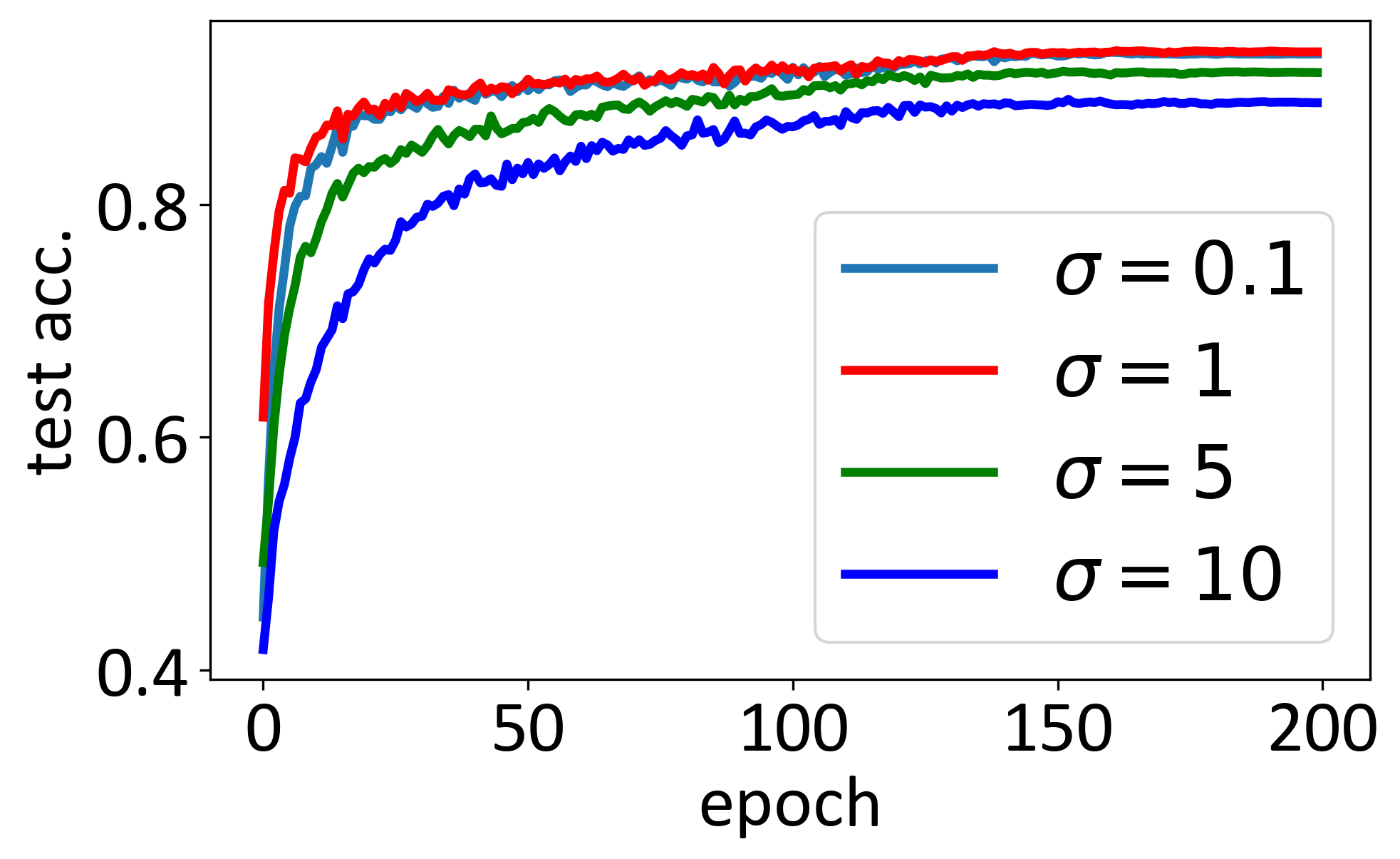
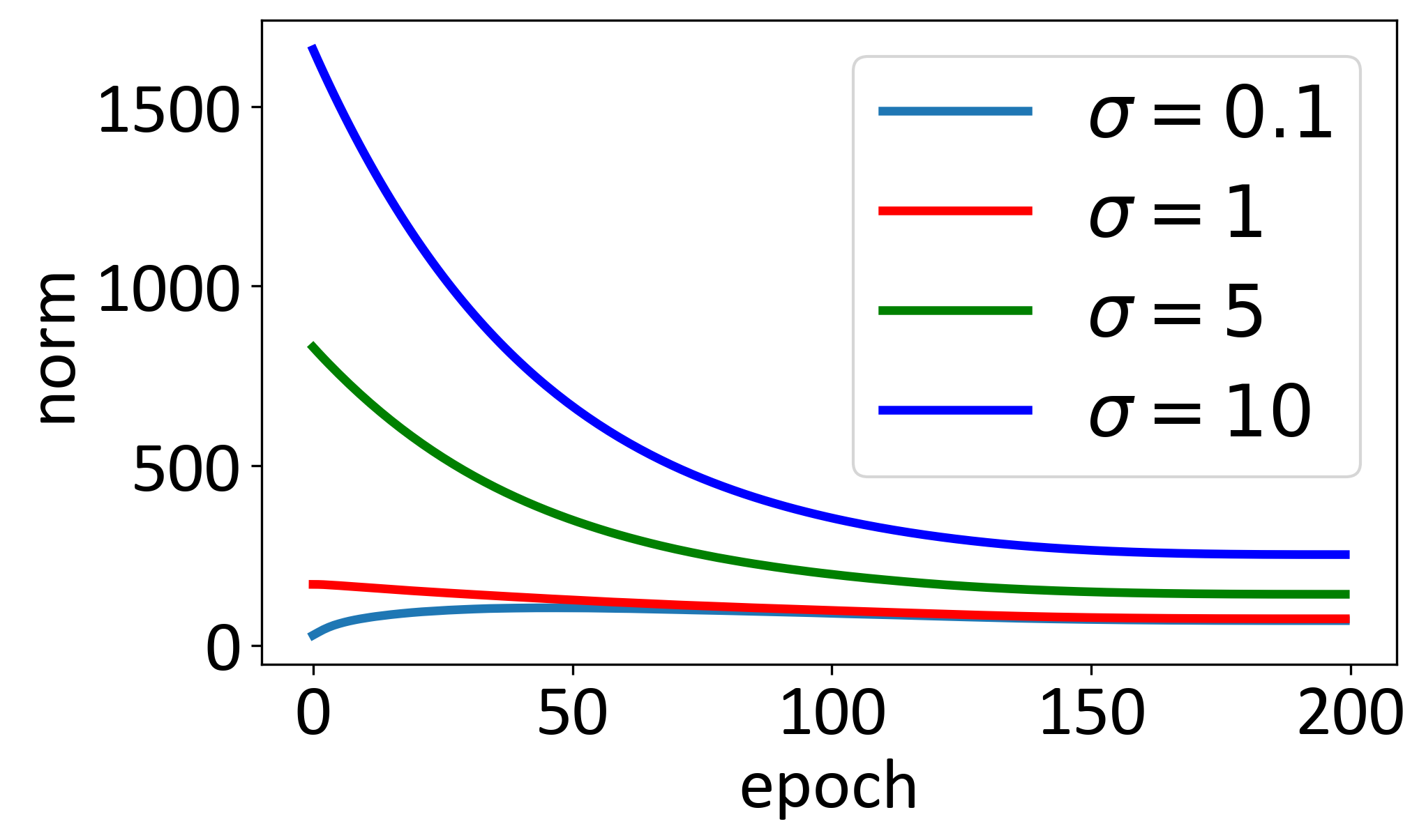
Figure 2: The initialization scale $\sigma$ correlates negatively with the performance of Resnet-18 on the CIFAR-10 dataset. Left: test accuracy. Here, $\sigma$ is a constant multiplier we apply to the initialized weights of the model under the Kaiming init. Right: the norm of all weights. While all models achieve a 100% training accuracy, models initialized at a larger scale converge to solutions with a larger norm, which is a sign that the layers are misaligned.

3 Phases Diagrams

Now, let us study the qualitative behaviors of the model when we scale the hyperparameters with a scaling parameter $\kappa$ towards infinity. Conventionally, the choice of $\kappa$ is the model width (for example, see Jacot et al., (2018) and Yang and Hu, (2020)); however, this excludes the discussion of the lazy training regime in the theory, because in lazy training, the model width is kept fixed and the scaling parameter is the model output scale $\gamma$. In this section, $\kappa$ is an abstract quantity that increases linearly, and all the hyperparameters including the width are a power-law function of $\kappa$. This allows us to discuss a much broader class of the scalings in the same framework than what has been achieved in Yang and Hu, (2020).

We first establish a necessary condition for learning to happen: the learning time $t_{c}$ needs to be of order $\Theta(1)$. When it diverges, learning is stationary and frozen at initialization. When it vanishes to zero, the discrete-time SGD algorithm will be unstable, a point that is first pointed out by Yang and Hu, (2020). Therefore, we first study the condition for $t_{c}$ to be of order $1$, which is equivalent to the condition that (assuming $x$, $y$ are order $1$)

$$\eta_{u}\eta_{w}\gamma^{2}+(\gamma^{2}d)^{2}PQ=\Theta(1).$$ (27)

We consider Gaussian initialization $u_{i0}\sim\mathcal{N}(0,\sigma_{u}^{2})$ and $w_{i0}\sim\mathcal{N}(0,\sigma_{w}^{2})$. Then $P,Q$ are random variables with expectation $(\eta_{w}\sigma_{u}^{2}+\eta_{u}\sigma_{w}^{2})/{4}$ and variance ${(\eta_{w}\sigma_{u}^{2}+\eta_{u}\sigma_{w}^{2})^{2}}/{8d}$. Generally, all hyperparameters are powers of $\kappa$: $d\propto\kappa^{c_{d}}$, $\gamma\propto\kappa^{c_{\gamma}}$, $\sigma_{w}^{2}\propto\kappa^{c_{w}}$, $\sigma_{u}^{2}\propto\kappa^{c_{u}}$, $\eta_{w}\propto\kappa^{c_{\eta_{w}}}$ and $\eta_{u}\propto\kappa^{c_{\eta_{u}}}$. For simplicity, we set the input dimension $d_{0}$ to be a constant.

Equation (27) implies

$$\max\left(2c_{\gamma}+c_{\eta_{u}}+c_{\eta_{w}},\ 2c_{\gamma}+c_{d}+\max\{c_{\eta_{w}}+c_{u},c_{\eta_{u}}+c_{w}\}\right)=0.$$ (28)

Whatever choice of the exponents that solves the above equation is a valid learning limit for a neural network. The phase of the network depends on the relative order of the above two terms.

Definition 1.

A model $f$ is in the kernel phase if (1) Eq. (18) is independent of $t$ as $\kappa\to\infty$ (2) $NTK=\Theta(1)$.

When $t_{c}=\Theta(1)$, a model is said to be in the feature learning phase if it is not in the kernel phase.

Theorem 2.

Let Eq. (28) holds, the network is in the kernel phase if and only if

$$\lim_{\kappa\to\infty}\frac{P}{Q}=1,\ a.s.$$ (29)

and

$$c_{d}+\max\{c_{\eta_{w}}+c_{u},c_{\eta_{u}}+c_{w}\}>c_{\eta_{u}}+c_{\eta_{w}}$$ (30)

The necessary condition (29) for the model being in the kernel phase is a very interesting condition, highlighting the paramount role of initialization in deep learning. There are three common cases when this is satisfied:

1. $d\to\infty$ and $u_{0}$ and $w_{0}$ are independent (standard NTK);

2. $d$ is finite and the initial model output is zero: $\sum_{i=1}^{d}\sum_{j=1}^{d_{0}}u_{i}w_{ij}x_{j}=0$ (conventional lazy training)

3. $d$ is finite, $\kappa\to\infty$ and $c_{u}+c_{\eta_{w}}\neq c_{w}+c_{\eta_{u}}$;

The first case is the standard way of initialization, from which one can derive the classic analysis of the kernel phase by invoking the law of large numbers. The second case is the assumption used in the lazy training regime (Chizat et al.,, 2018). (Chizat et al., (2018) assumes $c_{\gamma}=1$, $c_{\eta_{u}}=c_{\eta_{w}}=-2$ and $c_{u}=c_{w}=0$, satisfying the conditions of the exponents (28) and (30).) This case, however, relies on a special initialization, and thus our results better illustrate the occurrence of the kernel phase for advanced initialization methods where different weights can be correlated. The third case happens when the learning rate and the initialization are not balanced. This suggests that to achieve feature learning, one needs to pay utmost care to make sure that the learning rate and the initialization are well balanced: $c_{u}=c_{w}$.

In conclusion, the overall phase diagram is (1) kernel phase, if the first term in (28) is strictly smaller than the second term: $0=c_{\gamma}+c_{d}+\max\{c_{\eta_{w}}+c_{u},c_{\eta_{u}}+c_{w}\}>c_{\eta_{u}}+c_{\eta_{w}}$ and $\lim_{\kappa\to\infty}{P}/{Q}=1$, (2) feature learning phase if otherwise. A key difference between these two phases is whether the evolution of the NTK is $O(1)$, or equivalently whether the model learns features.

3.1 Phases Diagram of Infinite-Width Models

Now, let us focus on the case when $\kappa=d\to\infty$ (thus $c_{d}=1$), corresponding to the infinite width limit considered in the NTK and feature learning literature (Jacot et al.,, 2018; Li et al.,, 2020; Yang and Hu,, 2020). In this limit, $\lim_{\kappa\to\infty}{P}/{Q}=1$ naturally holds by law of large numbers. Therefore, a sufficient and necessary condition for the kernel phase is $0=c_{\gamma}+c_{d}+\max\{c_{\eta_{w}}+c_{u},c_{\eta_{u}}+c_{w}\}>c_{\eta_{u}}+c_{\eta_{w}}$.

scaling	NTK	mean field (Mei et al.,, 2018)	Xavier Init.	Kaiming Init.	lazy (Chizat et al.,, 2018)
$c_{d}$	1	1	1	1	0
$c_{\gamma}$	-1/2	-1	0	0	1
$c_{u}$	0	0	-1	0	0
$c_{w}$	0	0	-1	-1	0
$c_{\eta}$	0	0	0	0	0
phase	kernel	frozen	learning	unstable	unstable
$c_{\eta}^{*}$	0	1	0	-1	-2
phase	kernel	learning	learning	kernel	kernel
$c_{\eta}^{+}$	1	1	0	1	0
$c_{\gamma}^{+}$	-1	-1	0	-1	0
phase	learning	learning	learning	learning	learning
$c_{\eta}^{-}$	0	0	-2	-1	-2
$c_{\gamma}^{-}$	-1/2	-1/2	1	0	1
phase	kernel	kernel	kernel	kernel	kernel

Table 1: Phases of learning in different scaling limits. For brevity, the learning rates of the two layers are set to be equal. The first block shows that the models can be frozen or unstable if we do not scale $\eta$ accordingly. The second block shows that one can always choose $\eta$ such that the model training is stable and does not freeze. The third and fourth blocks show that one can always choose a pair of $\eta$ and $\gamma$ such that the model is in the feature learning phase or the kernel phase.

The following corollaries are direct consequences of Eq. (28).

Corollary 1.

For any $c_{\gamma}$, $c_{u}$ and $c_{w}$, choosing $c_{\eta_{u}}=c_{\eta_{w}}=\min\{-c_{\gamma},-2c_{\gamma}-c_{d}-\max\{c_{u},c_{w}\}\}$ ensures that the model is stable.

Corollary 2.

For any $c_{u}$ and $c_{w}$, choosing $c_{\eta_{u}}=c_{\eta_{w}}=c_{\eta}$ and $c_{\gamma}=-c_{\eta}$ with $c_{\eta}\geq c_{d}+\max\{c_{u},c_{w}\}$ leads to a feature learning phase.

Corollary 3.

For any $c_{u}$ and $c_{w}$, choosing $c_{\gamma}=-\frac{1}{2}(c_{d}+\max\{c_{u},c_{w}\}+c_{\eta})$ and $c_{\eta}<c_{d}+\max\{c_{u},c_{w}\}$ leads to a kernel phase.

While simple to prove, they imply two important messages: for every initialization scheme, (1) one can choose an optimal learning rate such that the learning is stable; (2) one can choose an optimal pair of learning rate and output scale $\gamma$ such that the model is in the feature learning phase. Point (1) agrees with the analysis in Yang and Hu, (2020), whereas point (2) is a new insight we offer. See Table 1 for the classification of different common scalings. We choose scalings according to Corollary 2 and 3, to turn each model into the feature learning or the kernel phase.

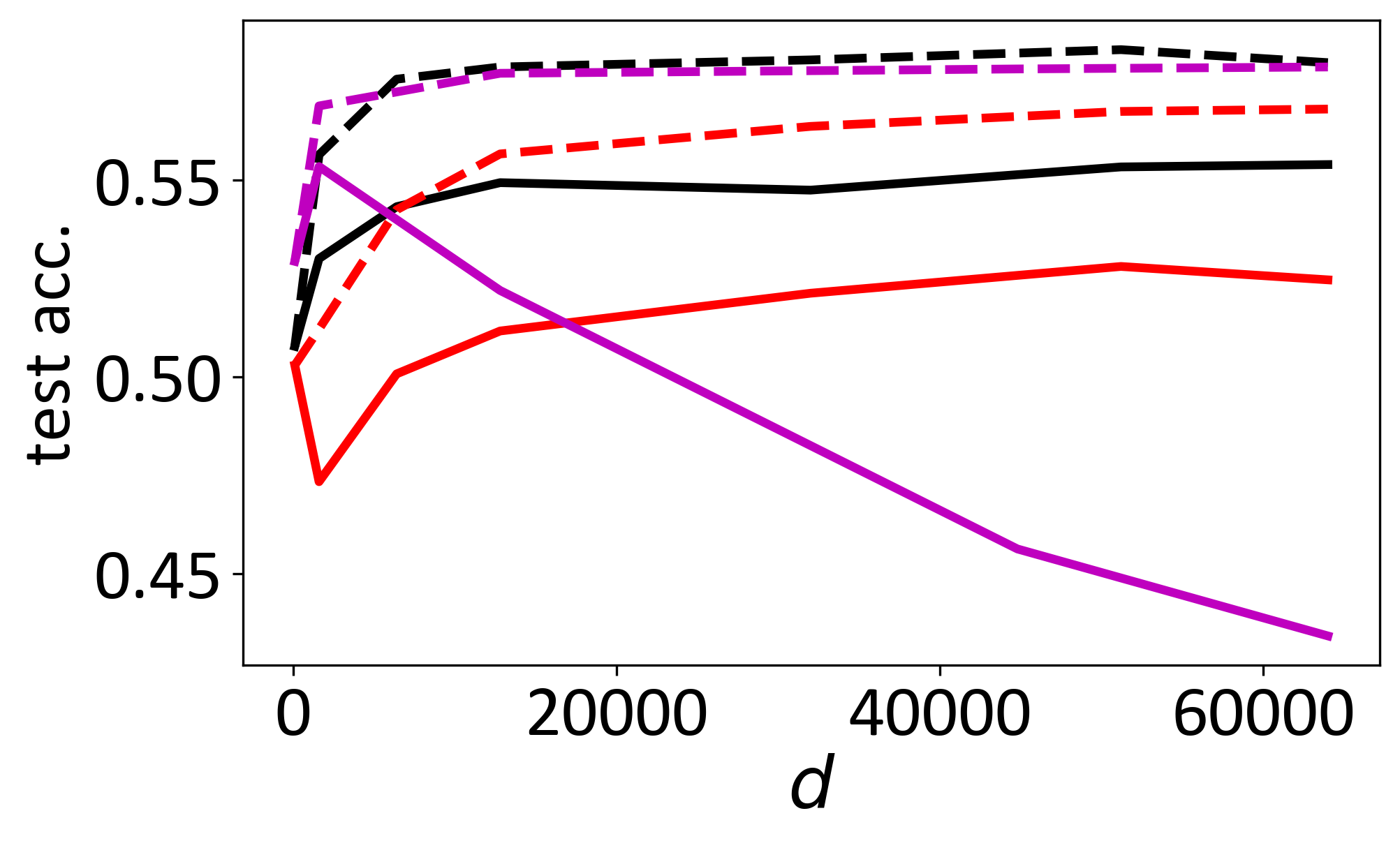
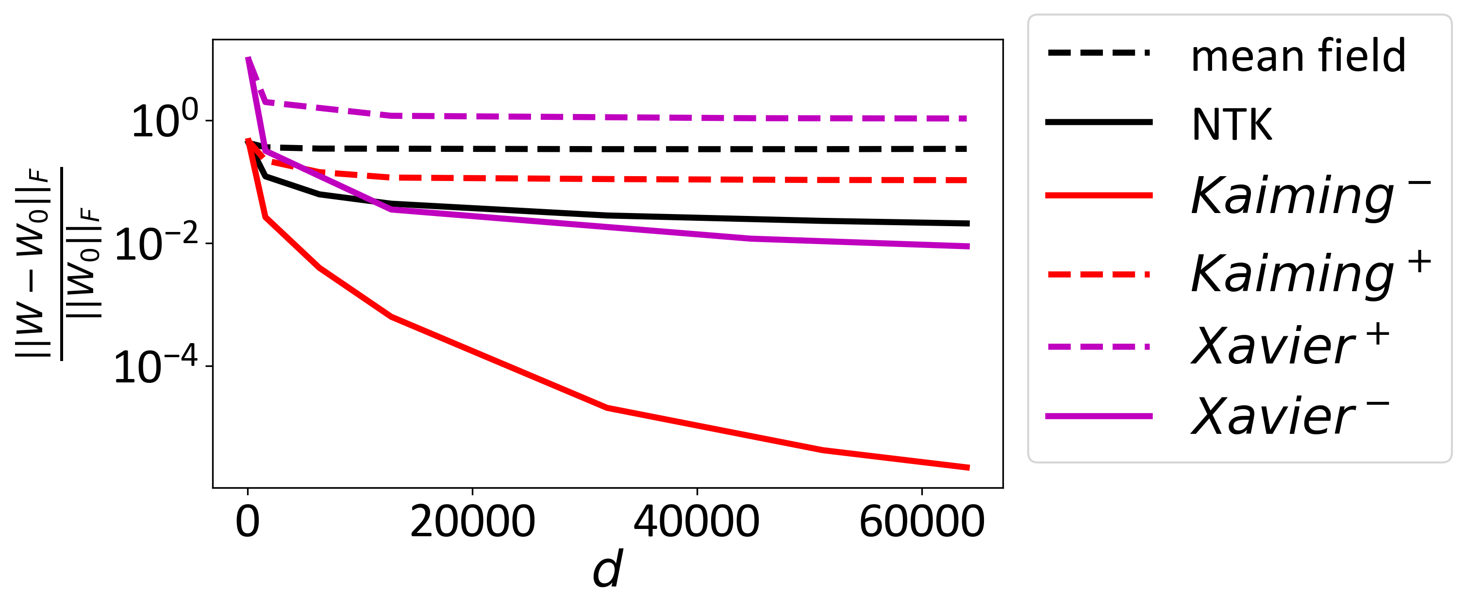
Figure 3: A two-layer fully connected ReLU net with $d$ neurons trained on the cifar10 dataset for $10000$ epochs with batchsize $128$. The kernel phase is shown in solid lines and the feature learning phase is shown in dashed lines. As the theory predicts, both types of initialization can be turned into either the feature learning or the kernel phase by choosing different combinations of $\gamma$ and $\eta$. Left: the best test accuracy during training. Right: relative distance from the initialization.

See Figure 3. We implement a two-layer fully connected network on the CIFAR-10 dataset. We run experiments with the scalings of the standard NTK, standard mean-field, Kaiming model and Xavier model. $c_{\gamma}$ and $c_{\eta}$ are chosen according to Table 1. For the Kaiming and Xavier model, we choose both $c_{\eta}^{\pm}$ and $c_{\gamma}^{\pm}$, and refer them as Kaiming^± and Xavier^±, respectively. The left figure shows that turning the Kaiming model into the feature learning phase improves the test accuracy by approximately $5\%$, similar to the gap between the standard NTK model and the mean field model. Meanwhile, turning the Xavier model into the kernel phase decreases the test accuracy by approximately $10\%$. This is because the fixed kernel restricts the generalization ability in the kernel phase, and the difference between these models in the kernel phase might be attributed to their different kernels. Thus, in agreement with the theory, choosing different combinations of the output scale $\gamma$ and $\eta$ can turn any initialization into the feature learning phase. This insight could be very useful in practice, as the Kaiming init. is predominantly used in deep learning practice and is often observed to have better performance at common sizes of the network. Our result thus suggests that it is possible to keep its advantage even if we scale up the network.

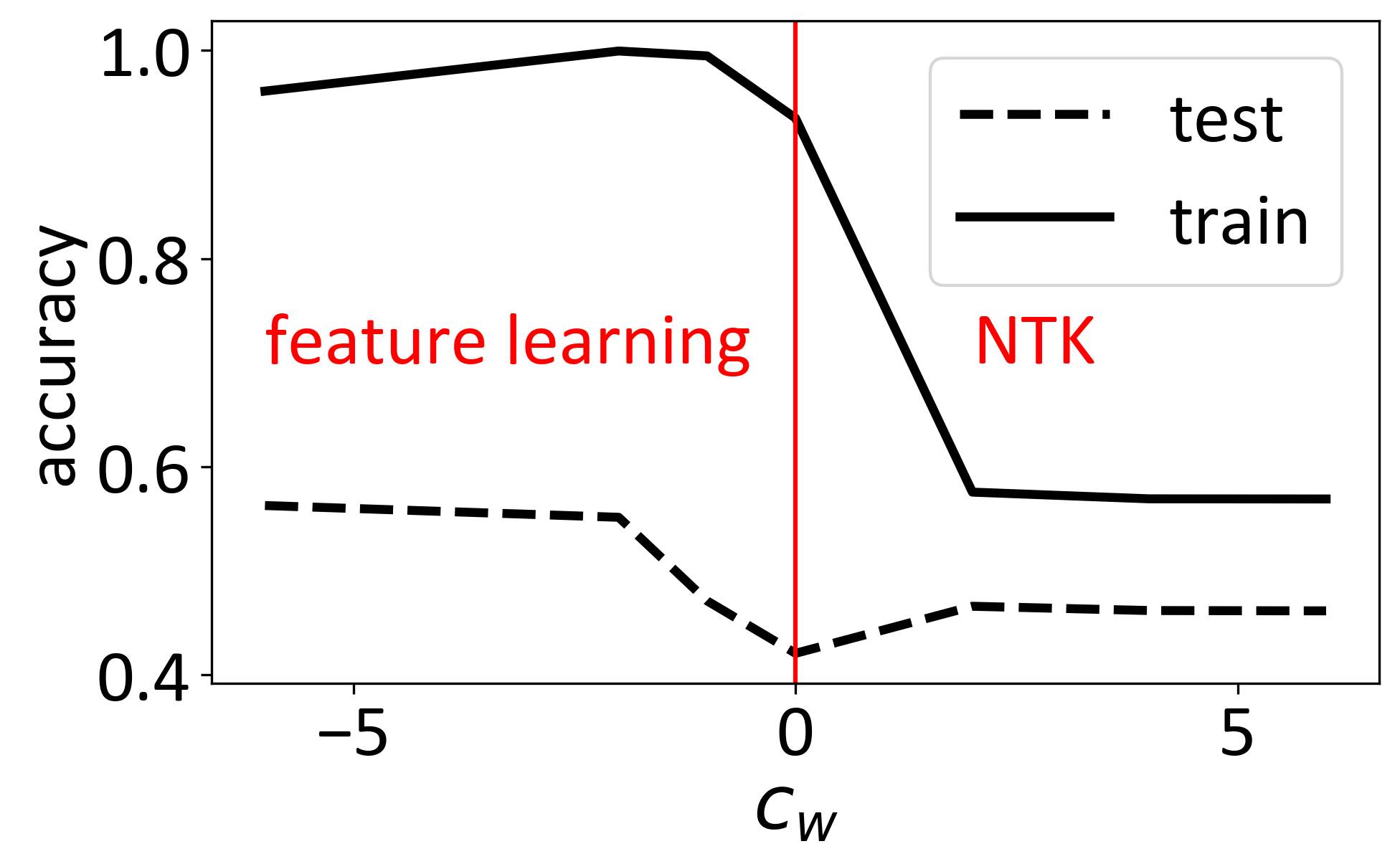
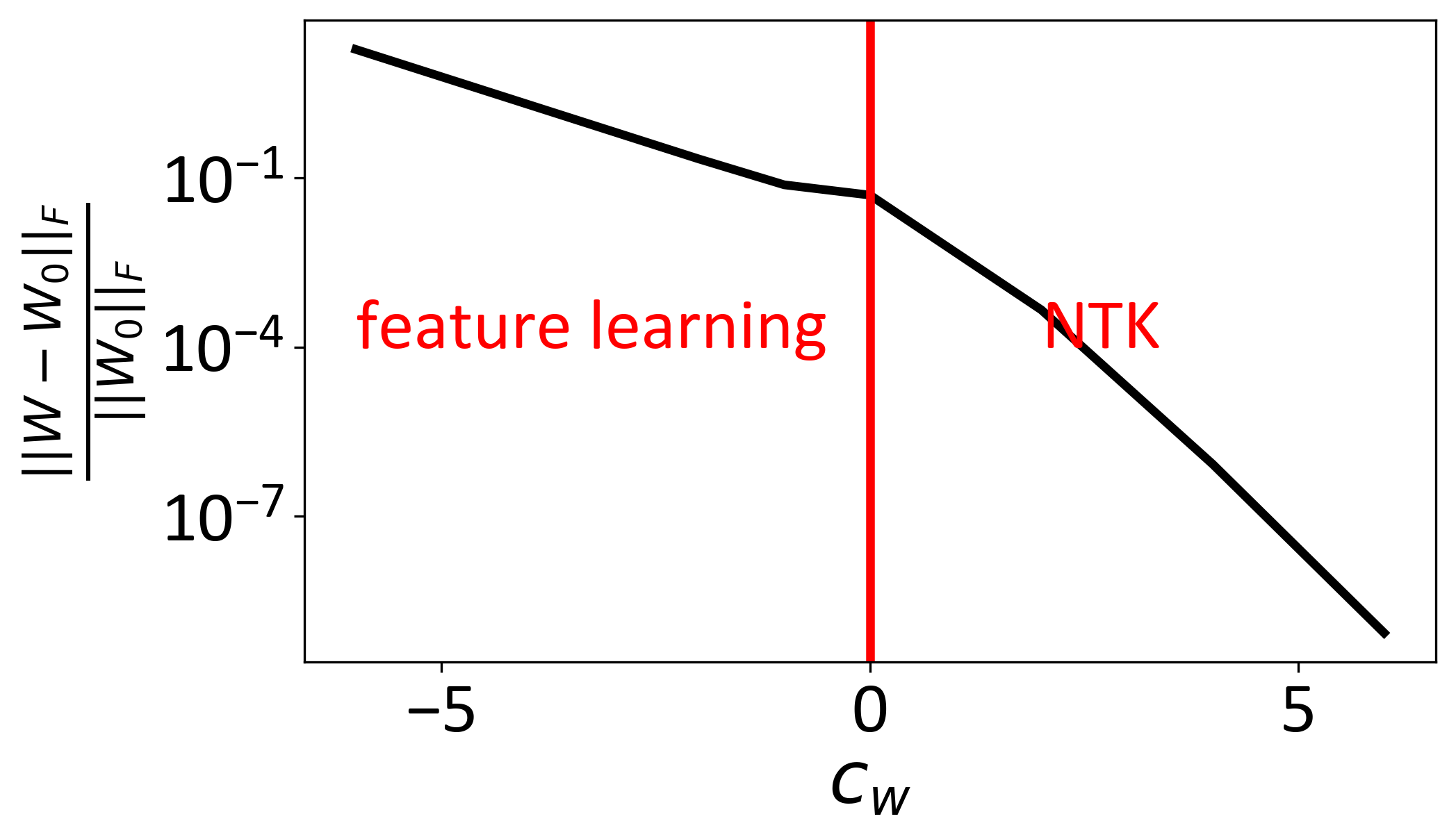
Figure 4: A two-layer fully connected network with different initialization scales trained on the CIFAR-10 dataset. We see that finite-sized models can also exhibit qualitative differences between the feature learning and the kernel phases when other hyperparameters are scaled toward infinity. Notably, this scaling is different from the lazy training scaling, implying that there are different (actually infinitely many) ways for the model to enter the kernel phase, even at a finite width.

3.2 Phase Diagram for Initializations

Now, we study the case when $d$ is kept fixed, while other variables scale with $\kappa\to\infty$. In this case, the phase diagram is also given by Theorem 2. See Figure 4 for an experiment. We set $c_{u}=\max\{0,c_{w}\}$ and $c_{\gamma}=\min\{-c_{w}/2,0\}$. This choice ensures that the initial model output is $O(1)$. In this case, (28) is satisfied. By Theorem 2, the network is in the kernel phase if and only if $c_{w}>0$.

Again, we implement a two-layer fully connected ReLU network on the CIFAR-10 dataset with $d=2000$. We choose $\kappa=10$ for illustration purposes. A clear distinction is observed between the feature learning phase and the kernel phase. (1) In Figure 4(a), the training accuracy can reach $1.0$ in the feature learning phase but not the kernel phase, because the NTK in the kernel phase is fixed, and thus the best training accuracy is limited by the fixed kernel. (2) As discussed in the previous section, the test accuracy In Figure 4(a) is about $5\%$ higher in the feature learning phase due to its trainable kernel. (3) In Figure 4(b), the weight matrices evolve significantly in the feature learning phase but not the kernel phase.

4 Conclusion

Solving for exactly solvable models has been a primary approach in theoretical sciences to understand how different controllable parameters are causally related to phenomena of interest. In this work, we have solved a minimal finite-size model of a two-layer linear network. Through a comprehensive analysis of its learning dynamics and phase diagrams, we have uncovered valuable insights into how feature learning happens and the impact of various scalings on the training dynamics of non-linear neural networks. Our theory is obviously limited. The first limitation is that the analytical results only hold for inputs lying in a one-dimensional subspace. This limitation arises from the potential inadequacy of conservation laws in more general cases (Marcotte et al.,, 2023), which we plan to explore further. Additionally, our findings regarding layer alignment and disalignment effects remain preliminary, necessitating a more in-depth analysis in the future. Lastly, it is worth considering how our results will become different when the gradient flow is replaced by stochastic gradient descent.

Appendix A Theoretical Concerns

A.1 Proof of Theorem 1

Proof.

By the definition of the gradient flow algorithm,

$$\frac{du_{i}}{dt}=-\eta_{u}\frac{\partial L}{\partial u_{i}}=-2\eta_{u}\gamma\sum_{j=1}^{d_{0}}w_{ij}x_{j}\left(\gamma\sum_{i=1}^{d}\sum_{j=1}^{d_{0}}u_{i}w_{ij}x_{j}-y\right),$$ (31)

$$\frac{dw_{ij}}{dt}=-\eta_{w}\frac{\partial L}{\partial w_{ij}}=-2\eta_{w}\gamma u_{i}x_{j}\left(\gamma\sum_{i=1}^{d}\sum_{j=1}^{d_{0}}u_{i}w_{ij}x_{j}-y\right),$$

which implies the following two conservation laws:

$$\frac{d}{dt}(\eta_{u}\sum_{j=1}^{d_{0}}w_{ij}^{2}-\eta_{w}u_{i}^{2})=0,$$ (32)

$$\frac{d}{dt}\left(\frac{w_{ij}}{x_{j}}-\frac{w_{ij^{\prime}}}{x_{j^{\prime}}}\right)=\frac{1}{x_{j}}\frac{dw_{ij}}{dt}-\frac{1}{x_{j^{\prime}}}\frac{dw_{ij^{\prime}}}{dt}=0.$$ (33)

From Eq. (31), we can denote $\frac{dw_{ij}}{dt}=u_{i}x_{j}A$, which implies

$$\frac{d}{dt}\left(\sum_{j=1}^{d_{0}}w_{ij}^{2}-\frac{1}{\sum_{j=1}^{d_{0}}x_{j}^{2}}(\sum_{j=1}^{N}w_{ij}x_{j})^{2}\right)=2\sum_{j=1}^{d_{0}}u_{i}w_{ij}x_{j}A-2\frac{\sum_{j=1}^{d_{0}}u_{i}w_{ij}x_{j}}{\sum_{j=1}^{d_{0}}x_{j}^{2}}\sum_{j=1}^{d_{0}}x_{j}^{2}A=0.$$ (34)

Now we denote $p_{i}(t):=\frac{1}{2\rho}(\sqrt{\eta_{u}}\sum_{j=1}^{d_{0}}w_{ij}(t)x_{j}+\sqrt{\eta_{w}}\rho u_{i}(t))$ and $q_{i}(t)\equiv:=\frac{1}{2\rho}(\sqrt{\eta_{u}}\sum_{j=1}^{d_{0}}w_{ij}(t)x_{j}-\sqrt{\eta_{w}}\rho u_{i}(t))$, and thus

$$p_{i}(t)q_{i}(t)=\frac{1}{4\rho^{2}}\left(\eta_{u}(\sum_{j=1}^{N}w_{ij}(t)x_{j})^{2}-\eta_{w}\rho^{2}u_{i}(t)^{2}\right).$$ (35)

Take derivatives on both sides and use (32) and (34). Then we have

$$\begin{aligned} \frac{d}{dt}\left(p_{i}(t)q_{i}(t)\right)&=\frac{1}{4}\frac{d}{dt}\left(\frac{\eta_{u}}{\sum_{j=1}^{d_{0}}x_{j}^{2}}(\sum_{j=1}^{N}w_{ij}x_{j})^{2}-\eta_{w}u_{i}^{2}\right)\\ &=\frac{1}{4}\frac{d}{dt}\left(\eta_{u}\sum_{j=1}^{d_{0}}w_{ij}^{2}-\eta_{w}u_{i}^{2}\right)=0\end{aligned}.$$ (36)

Further, substituting (31) into the definition of $p_{i}$ and $q_{i}$, we have

$$\frac{dp_{i}}{dt}=-2\gamma\sqrt{\eta_{u}\eta_{w}}p_{i}\rho\left(\sum_{j=1}^{d}(p_{j}^{2}-q_{j}^{2})\frac{\gamma\rho}{\sqrt{\eta_{u}\eta_{w}}}-y\right).$$ (37)

(37) implies $\frac{1}{p_{i}}\frac{dp_{i}}{dt}=\frac{1}{p_{i^{\prime}}}\frac{dp_{i^{\prime}}}{dt}$, further leading to another conservation law

$$\frac{d}{dt}\frac{p_{i}(t)}{p_{i^{\prime}}(t)}=0.$$ (38)

for all $i,i^{\prime}=1,2,\cdots,d$. Then according to (36) and (38), we have $p_{i^{\prime}}(t)=p_{i^{\prime}}(0)\frac{p_{i}(t)}{p_{i}(0)}$ and $q_{i^{\prime}}(t)=q_{i^{\prime}}(0)\frac{p_{i^{\prime}}(0)}{p_{i^{\prime}}(t)}$. Substituting them into (37), and we obtain a differential equation with only one variable $p_{i}$

$$\frac{dp_{i}}{dt}=-2p_{i}\left(\frac{(\gamma^{2}d)\rho^{2}P}{p_{i}(0)^{2}}p_{i}^{2}-\frac{(\gamma^{2}d)\rho^{2}Qp_{i}(0)^{2}}{p_{i}^{2}}-\gamma\rho y\sqrt{\eta_{u}\eta_{w}}\right),$$ (39)

where

$$P=\frac{1}{d}\sum_{i=1}^{d}p_{i}(0)^{2},\ Q=\frac{1}{d}\sum_{i=1}^{d}q_{i}(0)^{2}.$$ (40)

This differential equation is analytically solvable by integration

$$t=-\int_{p_{i}(0)^{2}}^{p_{i}^{2}}\frac{d\zeta}{4\left(\frac{(\gamma^{2}d)\rho^{2}P}{p_{i}(0)^{2}}\zeta^{2}-\gamma xy\sqrt{\eta_{u}\eta_{w}}\zeta-(\gamma^{2}d)\rho^{2}Qp_{i}(0)^{2}\right)}$$ (41)

Because the denominator as a quadratic polynomial has two different roots $\alpha_{\pm}$, the result of the integration is

$$t=-\frac{1}{4\sqrt{\eta_{u}\eta_{w}\gamma^{2}\rho^{2}y^{2}+4\rho^{4}(\gamma^{2}d)^{2}PQ}}\log\frac{p_{i}(t)^{2}/p_{i}(0)^{2}-\alpha_{+}}{p_{i}(t)^{2}/p_{i}(0)^{2}-\alpha_{-}}+const,$$ (42)

leading to

$$\frac{p_{i}(t)^{2}/p_{i}(0)^{2}-\alpha_{+}}{p_{i}(t)^{2}/p_{i}(0)^{2}-\alpha_{-}}=\frac{1-\alpha_{+}}{1-\alpha_{-}}\exp\left(-4\sqrt{\eta_{u}\eta_{w}\gamma^{2}\rho^{2}y^{2}+4\rho^{4}(\gamma^{2}d)^{2}PQ}t\right),$$ (43)

which gives (8). ∎

Proposition 1.

Under the condition in Theorem 1, if $P=0$ and $Q\neq 0$, the result becomes

$$p_{i}(t)=0$$ (44)

$$q_{i}(t)=q_{i}(0)\sqrt{\frac{\alpha^{\prime}\xi^{\prime}(t)}{1-\xi^{\prime}(t)}}$$ (45)

where

$$\xi^{\prime}(t):=\frac{1}{1+\alpha^{\prime}}\exp\left(-4\sqrt{\eta_{u}\eta_{w}}\gamma\rho yt\right),$$ (46)

and

$$\alpha^{\prime}:=\frac{\sqrt{\eta_{u}\eta_{w}}\gamma\rho y}{(\gamma^{2}d)\rho^{2}Q}.$$ (47)

Specially, if $P=Q=0$, we have $p_{i}(t)=q_{(}t)=0$, so the gradient flow will be stuck at the trivial saddle point.

The proof is similar to the proof of Theorem 1, because we can similarly obtain

$$\frac{dq_{i}}{dt}=-2q_{i}\left(\frac{(\gamma^{2}d)\rho^{2}Q}{q_{i}(0)^{2}}q_{i}^{2}+\gamma\rho y\sqrt{\eta_{u}\eta_{w}}\right).$$ (48)

Its solution gives Proposition 1.

We note that the behavior of the solution is quite different from $P\neq 0$: when $y\leq 0$, we can obtain a solution with zero loss in the end, but when $y>0$, the gradient flow will converge to the trivial saddle point $p_{i}=q_{i}=0$.

A.2 Proof of Theorem 2

Proof.

Using (29) and (30), we have

$$\lim_{\kappa\to\infty}\alpha_{+}=\lim_{\kappa\to\infty}\frac{2\rho^{2}(\gamma^{2}d)\sqrt{PQ}}{2\rho^{2}(\gamma^{2}d)P}=1.\ a.s.$$ (49)

By definition, $\xi(t)$ is a monotonic function. As $\frac{\alpha_{+}-\xi\alpha_{-}}{1-\xi}=\frac{\alpha_{+}-\alpha_{-}}{1-\xi}+\alpha_{-}$ is monotonous to $\xi$, it evolves from $1$ to $\alpha_{+}$ monotonously. Then according to Equation (18), $\lim_{\kappa\to\infty}K(x,x^{\prime})(t)=\lim_{\kappa\to\infty}K(x,x^{\prime})(0)$ if and only if $\lim_{\kappa\to\infty}\alpha_{+}=1$.

From Equation (28), Equation (30) also implies

$$2c_{\gamma}+c_{d}+\max\{c_{\eta_{w}}+c_{u},c_{\eta_{u}}+c_{w}\}=0.$$ (50)

Therefore, we can see that the NTK remains $\Theta(1)$ because

$$\gamma^{2}d\alpha_{+}P=\Theta(\kappa^{2c_{\gamma}+c_{d}+\max\{c_{\eta_{w}}+c_{u},c_{\eta_{u}}+c_{w}\}})=\Theta(1).$$ (51)

The proof is complete. ∎

Appendix B Additional Experimental Concerns

B.1 Additional Experiments in Section 2.2

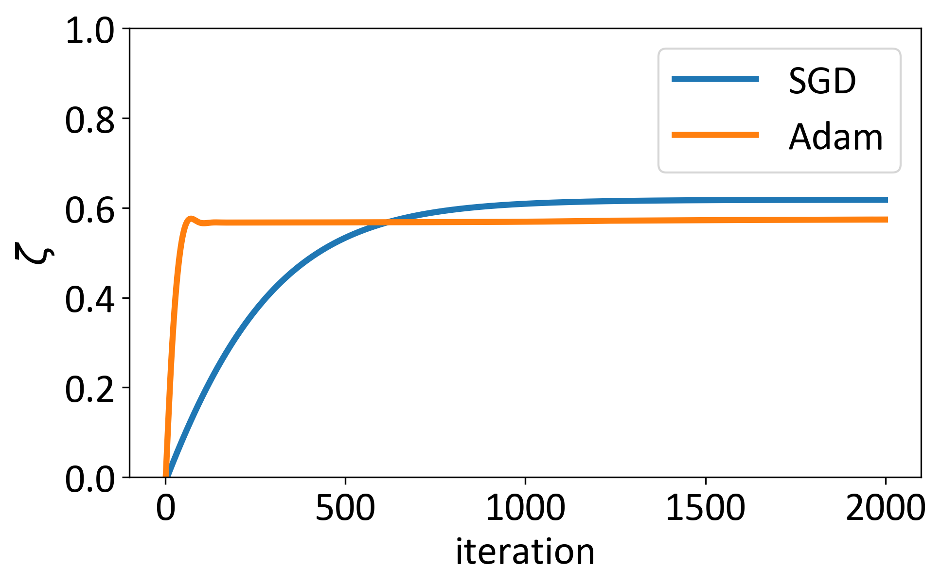
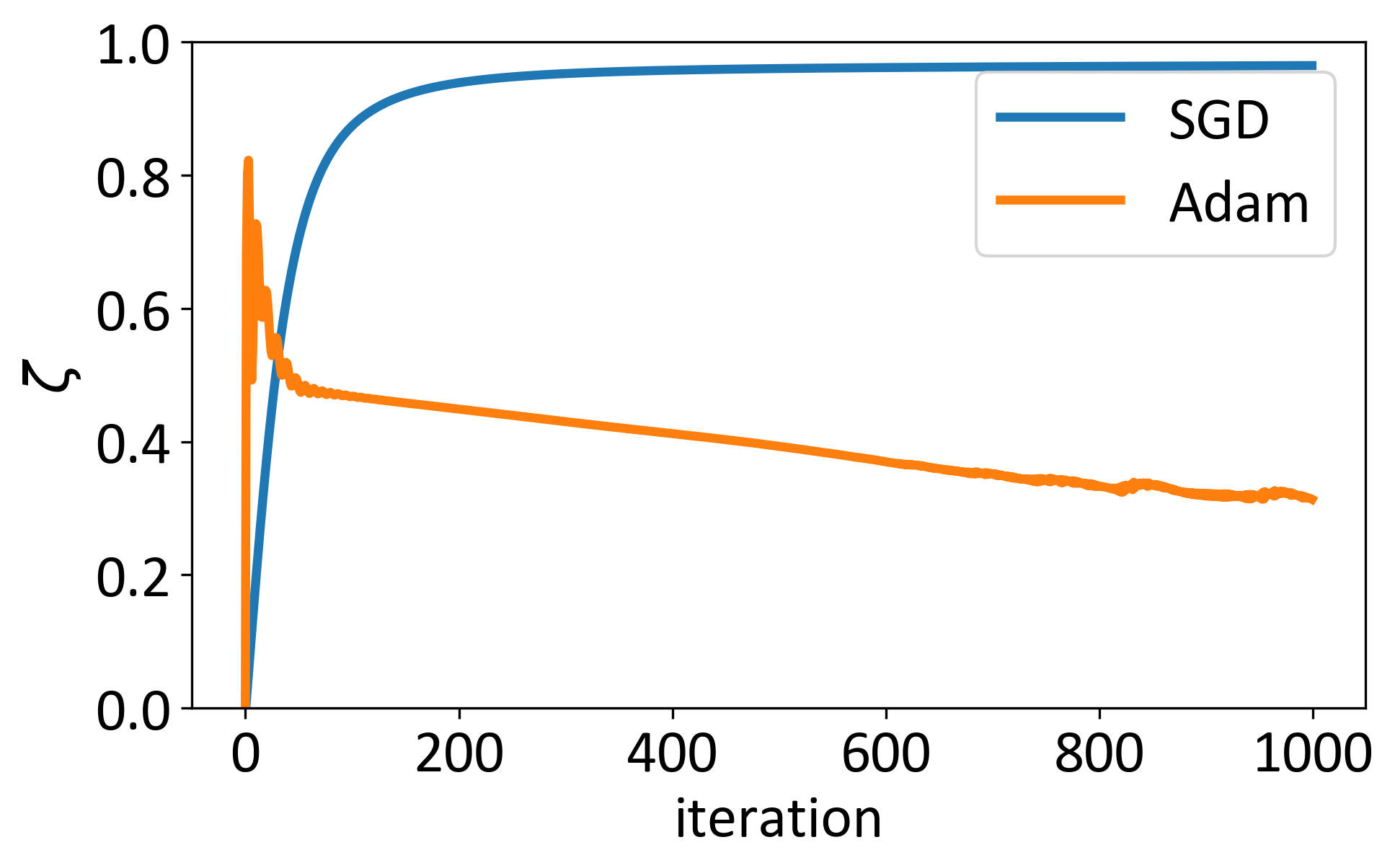
Figure 5: The evolution of the angle between $u$ and $v$ with Xavier⁺ and Kaiming⁺ initialization. Left: $Xavier^{+}$ initialization. Right: $Kaiming^{+}$ initialization.

In Figure 1 (a) and (b), we choose $x=1,y=2$. $\gamma=1/\sqrt{d}$ in the kernel phase and $\gamma=1/d$ in other cases. In (c) and (d), we randomly sample 100 points as $x$, and set $y=2x+noise$.

In addition, we also test the layer alignment and disalignment effect on a two-layer linear network with other kinds of initialization in Figure 5. We choose $\gamma=1$ in the Xavier⁺initialization and $\gamma=1/d$ in the Kaiming⁺ initialization. The settings in Figure 1 and Figure 5 are the same. Figure 5 further verifies the analysis in Section 2.2 that SGD and Adam converges to a similar solution in the Xaver⁺ solution where $\|u\|\approx\|w\|$, but SGD leads to a larger change in alignment in the Kaiming⁺ initialization where $\|w\|\ll\|u\|$.

B.2 Experiments in Section 2.3

In Figure 2, we train a Resnet18 network on the CIFAR-10 dataset with hyperparameters borrowed from https://github.com/kuangliu/pytorch-cifar. The only difference is that we scale each layer by $\sigma$ and record the test accuracy together with the sum of norm of all layers.

B.3 Experiments in Section 3.1

In Section 3.1, we utilize a two-layer fully connected network with the ReLU activation and $d$ hidden units. The input is vectorized and normalized, so the input dimension is $d_{0}=3072$. The cross-entropy loss and the stochastic gradient descent without moment or weight decay are used during training. We use a batch size of $128$ and report the best training and test accuracy among all epochs.

We choose $\gamma=\frac{1}{\sqrt{d}}$ and $\eta=0.05$ for the standard NTK model, $\gamma=\frac{10}{d}$ and learning rate $\eta=0.05d/100$ for the standard mean field model, $\gamma=1$ and $\eta=0.05d/100$ for the Kaiming^- model, $\gamma=\frac{100}{d}$ and $\eta=0.05d/100$ for the Kaiming⁺ model, $\gamma=1$ and $\eta=0.05$ for the Xavier⁺ model, $\gamma=0.01d$ and $\eta=0.05(100/d)^{2}$ for the Xavier^- model. The choice of hyperparameters guarantees that the standard NTK model and the standard mean-field model, the Kaiming⁺ and Kaiming^- model, and the Xavier⁺ and Xavier^- model are the same for $d=100$, respectively.

B.4 Experiments in Section 3.2

The experiment in Section 3.2 is similar to that in 3.1. The only difference is that we fix $d=2000$ and change the initialization scale. More specifically, we set $\kappa=10$, $\sigma_{u}^{2}=\kappa^{c}$, $\sigma_{w}^{2}=\kappa^{\max\{c,0\}}$ and $\gamma=\kappa^{-\min\{0,-c/2\}}$. We also fix $\eta=0.005$.

References

- Arpit et al., (2019) Arpit, D., Campos, V., and Bengio, Y. (2019). How to initialize your network? robust initialization for weightnorm & resnets. Advances in Neural Information Processing Systems, 32.
- Atanasov et al., (2021) Atanasov, A., Bordelon, B., and Pehlevan, C. (2021). Neural networks as kernel learners: The silent alignment effect. arXiv preprint arXiv:2111.00034.
- Baratin et al., (2021) Baratin, A., George, T., Laurent, C., Hjelm, R. D., Lajoie, G., Vincent, P., and Lacoste-Julien, S. (2021). Implicit regularization via neural feature alignment. In International Conference on Artificial Intelligence and Statistics, pages 2269–2277. PMLR.
- Bordelon and Pehlevan, (2022) Bordelon, B. and Pehlevan, C. (2022). Self-consistent dynamical field theory of kernel evolution in wide neural networks. Advances in Neural Information Processing Systems, 35:32240–32256.
- Chen et al., (2020) Chen, S., He, H., and Su, W. (2020). Label-aware neural tangent kernel: Toward better generalization and local elasticity. Advances in Neural Information Processing Systems, 33:15847–15858.
- Chizat et al., (2018) Chizat, L., Oyallon, E., and Bach, F. (2018). On lazy training in differentiable programming. arXiv preprint arXiv:1812.07956.
- Geiger et al., (2021) Geiger, M., Petrini, L., and Wyart, M. (2021). Landscape and training regimes in deep learning. Physics Reports, 924:1–18.
- Hanin and Nica, (2019) Hanin, B. and Nica, M. (2019). Finite depth and width corrections to the neural tangent kernel. arXiv preprint arXiv:1909.05989.
- Hu et al., (2020) Hu, W., Xiao, L., and Pennington, J. (2020). Provable benefit of orthogonal initialization in optimizing deep linear networks. arXiv preprint arXiv:2001.05992.
- Huang and Yau, (2020) Huang, J. and Yau, H.-T. (2020). Dynamics of deep neural networks and neural tangent hierarchy. In International conference on machine learning, pages 4542–4551. PMLR.
- Huang et al., (2020) Huang, W., Du, W., and Da Xu, R. Y. (2020). On the neural tangent kernel of deep networks with orthogonal initialization. arXiv preprint arXiv:2004.05867.
- Ioffe and Szegedy, (2015) Ioffe, S. and Szegedy, C. (2015). Batch normalization: Accelerating deep network training by reducing internal covariate shift. arXiv preprint arXiv:1502.03167.
- Jacot et al., (2018) Jacot, A., Gabriel, F., and Hongler, C. (2018). Neural tangent kernel: Convergence and generalization in neural networks. Advances in neural information processing systems, 31.
- Kingma and Ba, (2014) Kingma, D. P. and Ba, J. (2014). Adam: A method for stochastic optimization. CoRR, abs/1412.6980.
- Li et al., (2020) Li, Y., Ma, T., and Zhang, H. R. (2020). Learning over-parametrized two-layer neural networks beyond ntk. In Conference on learning theory, pages 2613–2682. PMLR.
- Liu et al., (2020) Liu, C., Zhu, L., and Belkin, M. (2020). On the linearity of large non-linear models: when and why the tangent kernel is constant. Advances in Neural Information Processing Systems, 33:15954–15964.
- Liu et al., (2022) Liu, Y., Mai, S., Chen, X., Hsieh, C.-J., and You, Y. (2022). Towards efficient and scalable sharpness-aware minimization. In Proceedings of the IEEE/CVF Conference on Computer Vision and Pattern Recognition, pages 12360–12370.
- Marcotte et al., (2023) Marcotte, S., Gribonval, R., and Peyré, G. (2023). Abide by the law and follow the flow: Conservation laws for gradient flows.
- Mei et al., (2018) Mei, S., Montanari, A., and Nguyen, P.-M. (2018). A mean field view of the landscape of two-layer neural networks. Proceedings of the National Academy of Sciences, 115(33):E7665–E7671.
- Radhakrishnan et al., (2022) Radhakrishnan, A., Beaglehole, D., Pandit, P., and Belkin, M. (2022). Feature learning in neural networks and kernel machines that recursively learn features. arXiv preprint arXiv:2212.13881.
- Saxe et al., (2013) Saxe, A. M., McClelland, J. L., and Ganguli, S. (2013). Exact solutions to the nonlinear dynamics of learning in deep linear neural networks. arXiv preprint arXiv:1312.6120.
- Simon et al., (2023) Simon, J. B., Knutins, M., Ziyin, L., Geisz, D., Fetterman, A. J., and Albrecht, J. (2023). On the stepwise nature of self-supervised learning. arXiv preprint arXiv:2303.15438.
- Sutskever et al., (2013) Sutskever, I., Martens, J., Dahl, G., and Hinton, G. (2013). On the importance of initialization and momentum in deep learning. In International conference on machine learning, pages 1139–1147. PMLR.
- Tieleman and Hinton, (2012) Tieleman, T. and Hinton, G. (2012). Lecture 6.5—RmsProp: Divide the gradient by a running average of its recent magnitude. COURSERA: Neural Networks for Machine Learning.
- Xu et al., (2019) Xu, Z.-Q. J., Zhang, Y., and Xiao, Y. (2019). Training behavior of deep neural network in frequency domain. In Neural Information Processing: 26th International Conference, ICONIP 2019, Sydney, NSW, Australia, December 12–15, 2019, Proceedings, Part I 26, pages 264–274. Springer.
- Yang and Hu, (2020) Yang, G. and Hu, E. J. (2020). Feature learning in infinite-width neural networks. arXiv preprint arXiv:2011.14522.
- Zhang et al., (2020) Zhang, Y., Xu, Z.-Q. J., Luo, T., and Ma, Z. (2020). A type of generalization error induced by initialization in deep neural networks. In Mathematical and Scientific Machine Learning, pages 144–164. PMLR.
- Ziyin et al., (2023) Ziyin, L., Li, H., and Ueda, M. (2023). Law of balance and stationary distribution of stochastic gradient descent. arXiv preprint arXiv:2308.06671.