Biofilms as poroelastic materials
Abstract. Biofilms are bacterial aggregates encased in a self-produced polymeric matrix which attach to moist surfaces and are extremely resistant to chemicals and antibiotics. Recent experiments show that their structure is defined by the interplay of elastic deformations and liquid transport within the biofilm, in response to the cellular activity and the interaction with the surrounding environment. We propose a poroelastic model for elastic deformation and liquid transport in three dimensional biofilms spreading on agar surfaces. The motion of the boundaries can be described by the combined use of Von Kármán type approximations for the agar/biofilm interface and thin film approximations for the biofilm/air interface. Bacterial activity informs the macroscopic continuous model through source terms and residual stresses, either phenomenological or derived from microscopic models. We present a procedure to estimate the structure of such residual stresses, based on a simple cellular automata description of bacterial activity. Inspired by image processing, we show that a filtering strategy effectively smooths out the rough tensors provided by the stochastic cellular automata rules, allowing us to insert them in the macroscopic model without numerical instability.
Keywords. Biofilm, poroelastic, Von Kármán, thin film, cellular automata, total variation based filter.
1 Introduction
The evolution of multicellular systems implicates biological, chemical and physical processes over a variety of spatial and temporal scales. At a microscopic level, cells are discrete entities which perform tasks (growth, division, differentiation, secretion of chemicals, motion, death) in response to continuous fields (concentrations of oxygen, nutrients and waste, flows, stresses). Simultaneously, individual cells aggregate to form clusters exhibiting collective behaviors. Being able to understand and to reproduce the dynamics of multicellular systems requires the introduction of adequate mathematical models, as well as suitable tools for their analysis and simulation.
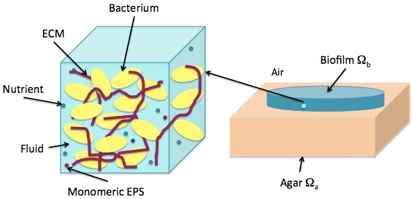
We consider here bacterial biofilms growing on agar/air interfaces. Roughly speaking, a biofilm consists of an elastic solid matrix (bacterial cells plus self produced polymeric meshwork) with inter-connected pores occupied by an extracellular fluid solution [1, 2]. Biofilms are known to provide mechanisms for antibiotic resistance [3] and constitute a main source of hospital acquired infections [4]. Understanding their structure may help to fight them.
For specific biofilms, such as those produced by Bacilus Subtilis, recent experiments suggest that the spread and shape of the biofilm is determined by the interplay of inner liquid transport and elastic deformations triggered by the cellular activity and by the interaction with the environment. Once bacteria adhere to a surface, they differentiate in several types in response to local variations created by growth, division, nutrient consumption, waste production, and cell-cell communication [5]. Some of them secrete exopolymeric substances (EPS) which form the extracellular matrix (ECM). EPS production changes the osmotic pressure within the biofilm, driving water from the agar substrate inside the film and fostering its spread on the surface [6]. Additionally, the polymeric matrix gives the biofilm a certain cohesion, allowing for measurements of elastic Young moduli. Localized death in regions of high density and high biochemical stress, combined with compression caused by division and growth, trigger the onset of wrinkle formation [7]. As the biofilm expands, complex wrinkled patterns develop. The occurrence of successive wrinkle branching and wrinkled coronas is related in [8] to stiffness gradients created by heterogeneous cellular activity and water migration. In later stages, the network of wrinkles becomes a network of channels which sustain the development of the biofilm transporting water, nutrients and waste [9]. The possibility of delamination and folding is analyzed in [10] by means of neo-Hookean models. We consider here the biofilm-substrate system as a block. Whereas biofilm spread due to water absorption from agar has been explained using two phase flow models and thin film approximations for the biofilm/air interface [6], wrinkle formation has been reproduced by means of plate Von Kármán equations for the biofilm/agar interface [8]. Seeking for a unified representation of both types of processes, we may consider poroelastic descriptions.
Poroelasticity studies the interaction of fluid flow and deformation in a fluid-saturated porous medium. This theory was proposed by Biot [11] in connection with soil consolidation models for the settlement of structures. It has later been applied to bone [12], tumor [13] and tissue [14] studies. There are three major approaches to the establishment of the main basic equations. The effective approach stems from solid mechanics. Effective parameters and constitutive laws are found averaging over representative volume elements [11, 15]. Instead, the mixture approach originates in the fluid mechanics tradition. Each position is occupied by particles of the different constituents of a mixture. The different species are assigned a density, stress, energy, and so on. Balance laws for the mass, momentum, and energy of each constituent are proposed, from which balance laws for the mixture are derived [2]. The basic equations provided by the mixture and the effective approach are similar. However, the mixture framework is advantageous when more than two constituents are present and in relative motion, see [16] for articular cartilage, for instance. In general, the mixture approach provides a better insight on fluid aspects whereas the effective approach allows for a better interpretation of parameters associated with the solid phase. A third homogenization approach [17] uses homogenization techniques to systematically derive macroscopic equations taking into account the microscopic structure, relating the effective parameters to the structure of the phases and analyzing wave propagation aspects of the theory. Depending on the volume fractions of fluid and solid, the dynamic viscosity of the fluid, the Lamé constants for the solid, the density of the solid, the hydraulic permeability of the fluid/solid system, the characteristic time for changes in the displacement of the solid, and the characteristic length of the system in the macroscopic scale, the fluid/solid system can be considered as monophasic viscoelastic, monophasic elastic, or truly biphasic mixture/poroelastic [2, 17, 18]. Applications of these models in geophysics [19, 20] and biomedicine [12, 13, 14] usually fix a spatial region and study the evolution of the different phases and physical magnitudes in it, avoiding to track moving boundaries, a relevant aspect to understand biofilm spread and shape.
In this paper, we propose a biphasic mixture/poroelastic description of biofilms spreading on agar surfaces which takes into account osmotic flow and incorporates nonlinear effects in the vertical displacements. This description should allow us to study simultaneously biofilm spread due to water intake from agar and the formation of wrinkles due to stiffness gradients. The motion of the two interfaces, the interface biofilm/agar and the interface biofilm/air is essential in these studies. We suggest effective equations for the dynamics of both interfaces.
The paper is organized as follows. Section 2 describes the equations for the deformation of the solid biomass and for the fluid flow, as well as the balance laws for the biomass and fluid phases and for the dissolved chemicals. Sections 3.1 and 3.2 propose reduced equations for the dynamics of the biofilm/agar and biofilm/air interfaces, respectively. Section 4 explains how to connect this model to stochastic discrete representations of cellular activity, such as cellular automata models. A mathematical procedure to generate smooth residual stresses from the cellular automata evolution which should then be plugged into the poroelastic equations is presented. Finally, Section 5 summarizes our conclusions.
2 Poroelastic description of a biofilm spreading on an agar/air interface
In this section, we propose a set of basic equations governing a biofilm in expansion on an air/agar interface. The biofilm occupies a region over an agar block , see Fig. 1. In principle, the biofilm is formed by bacterial cells, EPS matrix and interstitial fluid. Bacilus Subtilis cells differentiate into different kinds in a biofilm [5] (normal cells, surfactin producers, EPS producers, inert cells) and may also die. Moreover, the fraction of EPS matrix in the mixture depends on the type of bacteria. In biofilms formed by Pseudomonas strains spreading in flows, bacteria are scattered in large fractions of extracellular material [21]. Instead, in the biofilms formed by Bacilus Subtilis considered here, bacteria are densely packed, glued together by small fractions of extracellular material [6, 7]. This suggests considering a volume fraction of biomass that includes the volume fraction of cells and ECM (extracellular matrix):
Assuming that no voids neither air bubbles form inside the biofilm, the mixture is fully saturated, and the volume fraction of fluid is given by
| (1) |
The values of densities measured for tissues and agar do not differ much from the density of water (relative differences of order ). Therefore, we will also take the densities of all components to be constant and equal to that of water [6]: Fluid flow in the biofilms under consideration is a combination of Darcy and osmotic flow [6]. The equations for a poroelastic material in which water flow is a combination of Darcy and osmotic flow, caused by diffusion of a certain chemical, are given in [19, 20]. We revise them next in a more general context, incorporating biomass production due to nutrient consumption.
(a) (b)
2.1 Elastic deformations
Inspired by [22] and [20], Ref. [19] proposes a constitutive stress-chemical concentration-strain relationship between the volumetric strain increment , the effective mean stress increment and the osmotic pressure increment :
where is total mean stress (positive in tension), is the excess pore fluid pressure (positive in compression) and the osmotic pressure (positive in compression). The osmotic pressure created by a chemical concentration in solution is approximated by the Van’t Hoff equation:
| (2) |
where is a gas constant, the absolute temperature, and the molar mass of the solute. The resulting stress-strain relation for an isotropic medium is [19, 20]:
| (3) |
where is the displacement vector of the biomass and the deformation tensor:
| (4) |
The parameters and are the Lamé constants of the biomass, related to the Young and Poisson moduli by
| (5) |
The values of and depend on assumptions made about incompressibility and properties of the constituents [20, 19]. When the fluid/solid system is incompressible [2], . The tensor represents residual strains in the biomass created by growth, swelling or other processes [8].
The motion of the system should then be governed by the evolution equations
| (6) |
being the density of the medium and the body force. We fix the displacements at the agar/biofilm interface, while imposing no stress boundary conditions at the air/biofilm interface. Inertial terms are often neglected for tissues.
We can study the whole biofilm-agar system applying equation (6) and the constitutive law (3) to both domains . Then, we must solve (6) with coefficients varying sharply (possibly discontinuous) at the agar/biofilm interface, imposing transmission conditions at the interface and fixed displacements on the agar boundary. This is a standard situation in elasticity that can be handled numerically by finite elements, for instance, but it is quite costly and poses technical difficulties related to the presence of moving interfaces and contact fronts. Similar remarks hold for the equations formulated next in Sections 2.2-2.4. Within this framework, we could also consider biofilm delamination from agar as done for composite materials [23] if needed. Here we choose to focus on situations in which the biofilm remains attached to the agar substratum to cut the computational complexity by using effective equations for the moving biofilm boundaries.
2.2 Fluid flow
The fluid flow through pores is the combination of Darcy flow driven by standard pressure:
| (7) |
where is the hydraulic permeability (, permeability of the solid, fluid viscosity), and osmotic flow driven by osmotic pressure:
| (8) |
where is the osmotic efficiency. The total flow is [19]:
| (9) |
The previous effective equations for the fluid flow and the biomass deformation can be related to the momentum balance for the constituents of the mixture
| (10) |
using the following constitutive equations for the stress tensors [2, 24]
| (13) |
and a constitutive equation for the interaction force [2, 24]
| (14) |
The saturation condition implies expected to be small here. The concentration forces satisfy see [24]. The velocities are related to the displacements by , In the presence of gravity, the body forces are equal to the gravity force .
Assuming incompressibility of both phases, and disregarding the inertial terms (local accelerations) and the viscous contributions in the fluid stress tensor, the momentum balance laws yield:
| (17) |
The second equation provides a law for fluid flow:
| (18) |
which is related to (9) setting [25] and On the other hand, adding up the equations (17) we find effective equations for the displacements [24]:
| (20) |
2.3 Mass balance for biomass and fluid fractions
Assuming constant and equal density for all the components, the balance laws for the fractions of biomass and liquid are given by [19, 6]:
| (21) | |||
| (22) |
where represents biomass production due to nutrient consumption and is the biomass velocity. The displacements are computed from the equations for the stress in Section 2.1. The velocity of the fluid is
| (23) |
Equation (21) is supplemented with zero boundary conditions when , being the outer normal vector. Equation (22) requires boundary conditions when . We set the fluid volume fraction equal to zero when this happens at the interface with air, and equal to a given value at the interface with agar. To be more realistic, (22) should be coupled to a similar system for water dynamics in agar [6] using transmission conditions at the biofilm/agar interface and given volume fractions at the agar border.
A simple expression for biomass production is the Monod law [6]:
| (24) |
where is the nutrient concentration, the corresponding half-saturation constant and is the production rate, approximated by , being the doubling time for bacteria and a correction representing EPS production.
Adding up both conservation laws we find a balance equation for the whole growing mixture:
| (25) |
where is the composite velocity of the mixture. The relative velocity is then
| (26) |
where the permeability is often taken to be of the form [14, 6]
| (27) |
Here, is a friction parameter, the fluid viscosity and a representative bacterial radius. This expression for follows from Stokes theory of viscous drag applied to the biomass mixture, see [2] for other choices. The resulting balance equations for both phases are similar to those proposed in [6], except for the fact that the osmotic pressure created by the concentration enters the relative velocity and we have an equation for , the velocity being computed as .
2.4 Mass balance for chemicals
Effective continuity equations for chemical concentration in tissues are presented in [14]. For the limiting concentration :
| (29) |
where is an effective diffusivity [26]. Denoting by and the diffusivities in the biomass and liquid phases , The source represents consumption by the biofilm
| (30) |
being the uptake rate and the half-saturation constant. Zero flux boundary conditions are imposed at the air/biofilm interface. Instead, at the agar/ biofilm interface, we may impose a constant concentration through a Dirichlet boundary condition. Being more realistic, we will couple this diffusion equation to another one defined in the agar substratum with zero source and transmission conditions at the interface [8].
The polymeric substances secreted by the cells admit different treatments. In principle, we have a concentration of monomers which interact to form polymers of increasing length. The dissolved concentration of monomers may be selected as the concentration driving the osmosis process. It obeys an effective equation:
| (31) |
where is an effective diffusivity, as before. The source represents monomer production by the biofilm bacteria:
| (32) |
being the production rate and a maximum cut-off value. In practice we should substract a term representing the monomers that become polymers and form the matrix that we have included in the biomass. Zero flux boundary conditions are imposed at the air/biofilm interface. At the agar/biofilm interface, we may either impose zero flux boundary conditions, or couple this diffusion equation to another one defined in the agar substratum with zero source and transmission conditions at the interface.
Alive cells generate waste products which may hinder growth, causing damage and death [7, 3]. The evolution of the concentration of waste in the biofilm may be described by
| (33) |
where , being the waste production rate. Zero flux boundary conditions are imposed at the interfaces with air and agar. Waste accumulation is only reduced if carried away by circulating fluids or if cells die. It may be necessary to distinguish at least two phases within the biomass Then, the mass balance equation (21) splits in
| (34) |
with . In equations (29),(31), must be replaced by in the source definitions (30),(32). The new sources are
| (35) | |||
| (36) |
where represents a rate of death and a reabsorption rate for dead cells.
As mentioned earlier [5, 8], the biomass is in fact composed of fractions of extracellular matrix , dead bacteria , and alive cells, which include inert bacteria , bacteria secreting EPS , bacteria secreting surfactin and bacteria which do not produce such substances and are able to divide in a normal way . In practice, we may have to distinguish the different species:
which would require introducing additional balance equations for the different fractions and their interaction.
3 Motion of the interfaces
The equations presented in Section 2 are suitable to represent elastic deformations and liquid transport in a biofilm. However, as the biofilm swells and deforms, its boundary moves. To simplify the study of the evolution of a three dimensional biofilm it is desirable to obtain reduced equations for the motion of its boundary. In our geometry, the boundary is formed by two interfaces: the interface agar/biofilm and the interface air/biofilm. Whereas the first one controls the formation of wrinkled shapes [8], the second one defines biofilm spread [6].
3.1 Von Kármán approximation for the agar/biofilm interface
Equations for the dynamics of the agar/biofilm interface follow using a Von Kármán type approximation, since the thickness of the biofilms is small compared to its radius. While initially flat, the displacements in the direction orthogonal to the interface may become large. Thus, the linear definition of the strain and stress tensors in (4) is replaced by
| (37) | |||||
which includes nonlinear terms, as well as residual strains caused by bacterial activity and residual stresses estimated averaging the osmotic pressure and fluid pressure contributions to the three dimensional biofilm in the law (3) in the out of plane direction. We denote the in-plane displacements by and the out of plane displacements of the interface by . The coordinates vary along the 2D projection of the 3D biofilm structure on the biofilm/agar interface. Identifying the biofilm with an elastic film growing on a viscoelastic agar substratum, the interface motion is governed by the equations [27, 8]:
| (38) | |||
| (39) |
where is the thickness of the viscoelastic agar substratum and , , its rubbery modulus, Poisson ratio, and viscosity, respectively. The bending stiffness is , being the initial biofilm thickness. Summation over repeated indexes is intended. Here, the first equation describes out-of-plane bending and the second one in-plane stretching for the displacements . Modified equations taking into account possible spatial variations of the parameters are given in [28].
Let us explain now how to estimate the residual strains A growing biofilm is in a state of compression due to cell division and, eventually, water absorption, or cell death. In terms of a growth tensor [29], the residual term and the residual strains are Plugging residual stresses with this structure into (38)-(39), we are able to reproduce wrinkle coarsening and opening up in radial branches observed in biofilms spreading on surfaces [8]. This phenomenon is associated with the expansion at certain speeds of compression fronts.
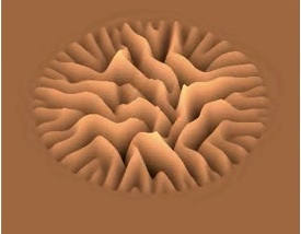
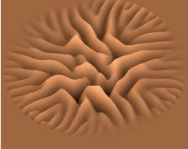
This approach does not impose a particular shape for the biofilm, which evolves as dictated by biomass production in response to variations in the concentration of nutrients, waste and autoinducers. However, simple illustrative simulations can be performed assuming a circular form. Often with If we assume that cells do not grow at expense of their neighbors, is a diagonal unit tensor in polar coordinates in a circular film. Setting for adequate velocities and constant or radially increasing profiles we obtain patterns like those in Fig. 2. Wrinkled coronas, that is, coronas of radial wrinkles issuing from a central core, are associated to the so-called corona instabilities: a swollen corona with diminished Young modulus around a harder core [8]. They can be reproduced imposing this spatial structure in the Young modulus in the Von Kármán equations.
(a) (b)
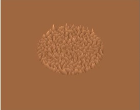
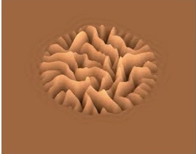
(c) (d)
Tracking the biofilm/agar interface by means of equations (38)-(39) forbids delamination, a phenomenon that has been reported in a variety of thin films coating surfaces [30]. Von Kármán theory is adapted in [30] to describe the evolution of films already debonded from a substratum forming blisters. [31] characterizes the onset of delamination in films whose edges are kept fixed while growing attached to a substrate. A situation closer to the geometry under study here is considered in [10] by means of a neo-Hookean elastic energy. If one follows branches of analytical solutions describing circular patches with a moderate adhesion which grow on a stiff substrate, contour undulations develop, buckling appears and, ultimately, a regular arrangement of folds emerges. In our setting, films can develop contour undulations [8], however, we do not consider delamination here.
3.2 Thin film approximation for the air/biofilm interface
The effective equations for the biofilm deformation in Section 2.1 govern , that is, the displacement of the biomass. However, the dynamics of the free air/biofilm interface is influenced by the displacement of liquids too. We obtain an equation for the motion of the interface air/biofilm using the mass balance equation for the mixture (28). During the first stages of biofilm spread, in which the agar/biofilm interface remains flat and the biofilm reaches a height , we integrate
in the vertical direction to get
, and being the unit vectors in the coordinate directions. By Leibniz’s rule:
Therefore
| (42) |
Notice that , . Differentiating with respect to time we find
Inserting this identity in (42) we obtain the equation
| (43) |
where
| (47) |
If the biofilm/agar interface is not flat, is replaced in the previous computations by an expression representing the height of this interface, calculated in Section 3.1. Additional terms representing the spatial variations of would appear in (43).
4 Coupling to discrete descriptions of cellular activity
In the previous sections cellular activity is represented through phenomenological sources and residual stresses. Alternatively, we may couple the equations for the macroscopic evolution of the biofilm to a discrete description of the cellular dynamics.
Cellular automata representations, for instance, furnish a simple approach which allows for an easy transfer of microscopic information into macroscopic models. We divide the biofilms in cubic tiles. Each of them contains a few bacteria. Further simplification of the computational geometry identifies each tile with one bacteria. Then, the matrix is a virtual glue that keeps bacteria together, which seems reasonable for biofilms on surfaces producing small fractions of EPS [6, 32]. This strategy will allow us to evaluate growth tensors due to cell activity (division, death, secretion, water absorption). They are defined on the cellular automata grid. We can use the same grid to discretize the equations for macroscopic concentrations and displacement fields. The residual stresses that enter the Föppl-Von Kármán equations for the deformation of the agar/biofilm interface can be computed from the growth tensor provided by the cellular automata descriptions. Instead, the air/biofilm interface changes now according to the cellular automata rules to create new tiles representing newborn bacteria, absorbed water or reabsorbed dead cells and displace the remaining tiles. The rules to decide the status of each tile may be based on probabilities depending on the pertinent concentrations [8] or dynamic energy budget models [3]. We sketch next the first approach.
4.1 Air/biofilm interface dynamics and rough residual strains
The evolution of the air/biofilm interface depends on the creation of new tiles and the displacement of existing ones. Assuming the nutrient is the concentration limiting biofilm growth, we set tiles occupied by alive bacteria to divide with probability [33]:
with . The concentration obeys an equation similar to (29) replacing with a weight equal to in alive cells and otherwise. Newborn bacteria push existing cells in the direction of minimum mechanical resistance, that is, the shortest distance to the air/bioiflm interface or to a dead cell.
As an indicator of death due to biochemical stress we chose the concentration of waste . A tile is scheduled to die with probability:
with . When surrounded by enough alive cells, dead cells may be reabsorbed by the rest, the tile being occupied by a newborn cell. Otherwise, a necrotic region is created [3]. The evolution of the concentration of waste in the biofilm is governed by equation (33), replacing with a weight equal to in alive cells and otherwise. A more sophisticated dynamic energy budget treatment of death processes can be found in [3].
Taking more autoinducer concentrations into consideration, we may define additional probabilities for other behaviors, such as differentiation cascades into autoinducer producers [8]. Probability laws using osmotic pressure would allow to create water tiles too [8].
(a) (b) (c)
(d) (e) (f)
Let us explain now how to calculate residual strains and stresses. Keeping track of all the new tiles created and the direction in which their predecessors where shifted, we are able to define a growth tensor . To do so, we introduce a vector where is the tile size. The component is calculated at each site by adding cumulatively for each tile shifted in the direction in the positive or negative sense, respectively. In a similar way, we calculate and along the and directions, respectively. Once the resulting vector is normalized to have norm , we evaluate approximating the derivatives by finite differences. Finally, we average all the contributions from over to obtain . However, stochastic variations make this tensor unsuitable to be inserted in the Föppl-Von Kármán equations (38)-(39), because of numerical instability.
4.2 Smooth residual strains and agar/biofilm interface dynamics
An effective way to smooth out the residual strains is to filter them by image processing techniques, which in addition visualizes the underlying spatial structure. To do so we formulate a denoising problem: given an observed magnitude , we seek the primary structure by removing the noise . This problem can be solved applying a split Bregman method to a ROF (Rudin-Osher-Fatemi) variational model [34, 35]: Find minimizing for large. The split Bregman method incorporates the constraint , sets and implements the iteration:
with . The minimization procedure solves for each variable alternatively:
Since the first functional is differentiable, we write the Euler-Lagrange equation and compute by a Gauss-Seidel method. To solve the second optimization problem we use shrinkage operators:
This strategy leads to the algorithm:
-
•
Initial guess , ,
-
•
While
-
–
,
-
–
,
-
–
,
-
–
where, for
with
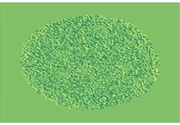
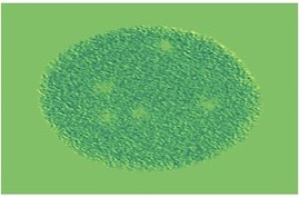
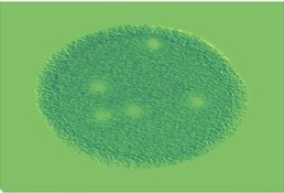
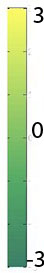
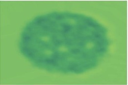
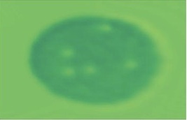
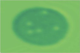
Fig. 3 computes the residual stresses for early stages of the evolution of an initially circular biofilm patch containing a few mounds, that is, regions where the biofilm is higher and contains more cells. In early stages, cell division affects mainly the biofilm height, in accordance with [6], though the circular shape may develop irregularities later [8, 10]. The filtered fields in Fig. 3(d)-(f) set over a 2D grid in the plane , relabeling to transform it into a 1D vector. Here, the ensemble averages of the residual strain tensors at trials are denoted by . At each trial we run the cellular automata step, in which new cells are created or killed according the the selected probabilities starting from the same initial configuration in all of them. For large enough these ensemble averages allow us to visualize the spatial variations caused by cellular activity, see Figure 3 (a)-(c). The resulting average becomes smoother as the number of runs increases. However, the remaining spikes still cause instability and the computational cost of this process is very high. Instead, this filtering process always produces fields which are smooth enough to be plugged in (38)-(39) without causing numerical instability. Filtered fields also reproduce the correct underlying spatial structure for a very low number of runs , lowering drastically the computational cost.
In this framework, the simulations of biofilm behavior would alternate steps in which we update the configuration of biofilm tiles following the cellular automata rules and evaluate the resulting residual stresses, with steps in which the biofilm shape is deformed as determined by the Föppl-Von Kármán equations for the agar/biofilm interface in Section 3.1 (see [8] for details) and steps in which the poroelastic and concentration equations are solved to update pressure, displacement, velocity and concentration fields.
5 Conclusions
Three dimensional multicellular shapes arise through the interaction of mechanical forces and cellular activities. Bacterial communities furnish model systems for studying such interplay. We consider here biofilms growing on air/agar interfaces, which have been shown to adopt wrinkled shapes and undergo swelling processes while spreading in interaction with the agar substratum. We have proposed a poroelastic solid/fluid model for the elastic deformation of the biomass matrix and the transport of interstitial fluid within it. Analyzing the two distinguished interfaces defining the biofilm borders we have found two different descriptions for the evolution of each of them. Whereas the interface agar/biofilm is reasonably represented by Von Kármán type approximations, the interface air/biofilm seems to require lubrication type approaches for thin films. These developments take into account the cellular activity through phenomenological sources and residual tensors included in the macroscopic equations. Instead, we may consider a discrete model of cellular activity to justify such phenomenological terms. Coupling to a simple cellular automata representation of bacterial activity, one can define residual stress tensors. Image filtering techniques allow us to regularize them so that can be effectively used in macroscopic models without causing instability at low computational cost. Whereas the dynamics of the agar/biofilm interface can still be described by Von Kármán type equations containing such residual stresses, the dynamics of the air/biofilm interface is now determined by the cellular automata rules for creation and motion of grid tiles. Delamination effects are not considered here and would require further study.
Acknowledgements. This research has been supported by MINECO grants No. MTM2014-56948-C2-1-P and No. MTM2017-84446-C2-1-R.
References
References
- [1] H.C. Flemming, J. Wingender, The biofilm matrix, Nat. Rev. Microbiol. 8 (2010) 623-633.
- [2] G.E. Kapellos, T.S. Alexiou, A.C. Payatakes, Theoretical modeling of fluid flow in cellular biological media: An overview, Math. Biosci. 225 (2010) 83-93.
- [3] B. Birnir, A. Carpio, E. Cebrián, P. Vidal, Dynamic energy budget approach to evaluate antibiotic effects on biofilms, Comm. Nonl. Sci. Num. Sim. 54 (2018) 70-83.
- [4] N. Hoiby, T. Bjarnsholt, M. Givskov, S. Molin, O. Cioufu, Antibiotic resistance of bacterial biofilms, Int. J. Antimicrob. Agents 35 (2010) 322-332.
- [5] L. Chai, H. Vlamakis, R. Kolter, Extracellular signal regulation of cell differentiation in biofilms, MRS Bulletin 36 (2011) 374-379.
- [6] A. Seminara, T.E. Angelini, J.N. Wilking, H. Vlamakis, S. Ebrahim, R. Kolter, D.A. Weitz, M.P. Brenner, Osmotic spreading of Bacillus subtilis biofilms driven by an extracellular matrix, Proc. Nat. Acad. Sci. USA 109 (2012) 1116-1121.
- [7] M. Asally, M. Kittisopikul, P. Rué, Y. Du, Z. Hu, T. Çağatay, A.B. Robinson, H. Lu et al, Localized cell death focuses mechanical forces during 3D patterning in a biofilm, Proc. Nat. Acad. Sci. USA 109 (2012) 18891-18896.
- [8] D.R. Espeso, A. Carpio, B. Einarsson, Differential growth of wrinkled biofilms, Phys. Rev. E 91 (2015) 022710.
- [9] J. N. Wilking, V. Zaburdaev, M. De Volder, R. Losick, M.P. Brenner, D.A. Weitz, Liquid transport facilitated by channels in Bacillus subtilis biofilms, Proc. Natl. Acad. Sci. USA 110 (2013) 848-852.
- [10] M. Ben Amar, M. Wu, Patterns in biofilms: From contour undulations to fold focussing, EPL 108 (2014) 38003.
- [11] M.A. Biot, General theory of three-dimensional consolidation, J. Appl. Phys. 12 (1941) 155-164.
- [12] S.C. Cowin, Bone poroelasticity, J. Biomechanics 32 (1999) 217-238.
- [13] S.L. Xue, B. Li, X.Q. Feng, H. Gao, Biochemomechanical poroelastic theory of avascular tumor growth, J. Mech. Phys. Solids 94 (2016) 409-432.
- [14] R. Sacco, P. Causin, Ch. Lelli, M.T. Raimondi, A poroelastic mixture model of mechanobiological processes in biomass growth: theory and application to tissue engineering, Meccanica 52 (2017) 3273-3297.
- [15] J.R. Rice, M.P. Cleary, Some basic stress diffusion solutions for fluid-saturated elastic porous media with compressible constituents, Rev. Geophys. Space Phys. 14 (1976) 227-241.
- [16] W.M. Lai, J.S. Hou, V.C. Mow, A triphasic theory for the swelling and deformation behaviors of articular cartilage, J. Biomech. Eng. 113 (1991) 245-258.
- [17] R. Burridge, J.B. Keller, Poroelasticity equations derived from microstructure, J. Acous. Soc. America 70 (1981) 1140-1146.
- [18] T. Shaw, M. Winston, C.J. Rupp, I. Klapper, P. Stoodley, Commonality of elastic relaxation times in biofilms, Phys. Rev. Lett. 93 (2004) 098102.
- [19] G. Chen, D. Gallipoli, A. Ledesma, Chemo-hydro-mechanical coupled consolidation for a poroelastic clay buffer in a radioactive waste repository, Trans. Porous Med. 69 (2007) 189-213.
- [20] A. Ghassemi, A. Diek, Linear chemo-poroelasticity for swelling shales: theory and application, J. Petrol. Sci. Eng. 38 (2003) 199-212.
- [21] K. Drescher, Y. Shen, B.L. Bassler, H.A. Stone, Biofilm streamers cause catastrophic disruption of flow with consequences for environmental and medical systems, Proc. Nat. Acad. Sci. USA 110 (2013) 4345-4350.
- [22] S.L. Barbour, D.G. Fredlund, Mechanisms of osmotic flow and volume change in clay soils, Can. Geotech. J. 26, (1989) 551-562.
- [23] K. Alnefaie, Finite element modeling of composite plates with internal delamination, Composite structures 90 (2009) 21-27.
- [24] Y. Lanir, Biorheology and fluid flux in swelling tissues. I Bicomponent theory for small deformations, including concentration effects, Biorheology 24 (1987) 173-187.
- [25] G. Oster, C.S. Peskin, Dynamics of osmotic fluid flow, in T.K. Karalis (eds), Mechanics of swelling, NATO ASI Series 64, 731-742 Springer, 1992.
- [26] B.W. Wood, M. Quintard, S. Whitaker, Calculation of effective diffusivities for biofilms and tissues, Biotech. Bioeng. 77 (2002) 495-516.
- [27] R. Huang, S.H. Im, Dynamics of wrinkle growth and coarsening in stressed thin films, Phys. Rev. E 74 (2006) 026214.
- [28] S. Iakunin, L.L. Bonilla, Variational formulation, asymptotic analysis, and finite element simulation of wrinkling phenomena in modified plate equations modeling biofilms growing on agar substrates, Comput. Methods Appl. Mech. Eng. 333 (2018) 257-286.
- [29] J. Dervaux, P. Ciarletta, M. Ben Amar, Morphogenesis of thin hyperelastic plates: A constitutive theory of biological growth in the Foppl-von Kármán limit, J. Mech. Phys. Solids 57 (2009) 458-471.
- [30] G. Gioia, M. Ortiz, Delamination of compressed thin films, Adv. Appl. Mech. 33 (1997) 119-188.
- [31] G. Napoli, S. Turzi, The delamination of a growing elastic sheet with adhesion, Meccanica 52 (2017) 3481-3487.
- [32] T. Storck, C. Picioreanu, B. Virdis, D.J. Batstone, Variable cell morphology approach for individual-based modeling of microbial communities, Biophys. J. 106 (2014) 2037-2048.
- [33] S.W. Hermanovic, A simple 2d biofilm model yields a variety of morphological features, Math. Biosci. 169 (2001) 1-14.
- [34] A. Torres, A. Marquina, J.A. Font, J.M. Ibáñez, Total-variation-based methods for gravitational wave denoising, Phys. Rev. D 90 (2014) 084029.
- [35] T. Goldstein, S. Osher, The split Bregman method for L1-regularized problems, SIAM J. Imaging Sci. 2 (2009) 323-343.