Interaction of Vortex Ring with Perforated V-Wall

Abstract

Experiments are performed to investigate the interaction of a vortex ring (Reynolds number based on circulation (Re_Γ = 11500) with perforated surface (open area ratio, $\phi_{1}=0.24$ and $\phi_{2}=0.44$) with different included angles ($\theta$ = 60° - 180° ). The phenomenon is characterized using techniques like Planer Laser-Induced Fluorescence (PLIF) imaging and Particle Image Velocimetry (PIV). Lagrangian analysis using finite-time Lyapunov exponents (FTLE) and $\Gamma_{2}$ vortex identification methods are utilised to understand the flow physics. Early observations reveal the growth of induced mushroom structures through the holes as a consequence of placing the perforated surface in the path of the vortex ring. These structures along with Kelvin-Helmholtz (K-H) instability imparts the initial instability to the emerging jets. We discern a sequential emergence of the vortex ring in the form of jets at lower $\theta$ value that diminishes at higher values. Except for $\theta$ = 150° cases, where the flow from the two halves starts to talk resulting in a divergence in the circulation ratio, a reformed vortex ring is formed for all cases in the far downstream. A detailed discussion on the downstream vorticity dynamics has been been provided using vorticity contours, time-series variation of circulation and the FTLE fields. By varying the value of $\theta$, we present a more generalised study of vortex ring interacting with perforated surfaces that finds application in multiple domains including flow control, manipulation and vortical cleaning.

1 Introduction

Vortex rings are formed as a result of an impulsive motion of fluid mass leading to the rolling up of shear layers at the corner of the pipe/hole used to generate it. They are fluidic structure that are of industrial as well as fundamental importance. In nature, they can be observed in smoke rings, jellyfish locomotion (Dabiri et al., 2005), wakes of flying birds (Wolf et al., 2013), mushroom clouds during volcanic eruptions and explosion (Lim & Nickels, 1995), micro-burst (Lundgren et al., 1992), cardiac relaxation of human heart (Per M. et al., 2016), and more. Application wise, they can be used for flow control purposes (Amitay et al., 2001; You & Moin, 2008), heat transfer application of jets (Liu & Sullivan, 1996; Hadziabdic & Hanjalic, 2008), particle shaping technique (An et al., 2016), and cleaning purposes (Jain et al., 2023) to name a few.

From a long time, physicists have been intrigued in understanding the fundamental behaviour of vortex ring and the interplay of its origin and decay with the surrounding. Works by Saffman (1970); Maxworthy (1972, 1977); Didden (1979); Glezer (1988); Glezer & Coles (1990) includes investigations on the fundamental aspects of vortex ring like the translation velocity, laminar and turbulent natures, their stability and formation. More recent works by Gharib et al. (1998); Mohseni & Gharib (1998); Shusser & Gharib (2000); Gan et al. (2012); Krieg & Mohseni (2013); Xiang et al. (2017) shows the existence of a universal formation number, discusses formation time scales, drag forces, modelling of translation properties and energy of the vortex ring.

Of interest to the present work is how vortex rings interact with other bodies like vortex ring itself, solid or porous surfaces and fluidic interfaces. Lim & Nickels (1992); Cheng et al. (2018) reported the collision of a vortex ring with another vortex ring giving rise to vortex reconnection and multiple small sized vortex rings. The interaction of vortex ring with a flat wall normal and inclined to the translation axis of vortex ring has been reported (Walker et al., 1987; Lim, 1989; Orlandi, 1990; Chu et al., 1993; Couch & Krueger, 2011; New et al., 2016). Interactions with round cylinders (Naitoh et al., 1995; New & Zang, 2017), sphere (ALLEN et al., 2007) ,V-shaped wall (New et al., 2020), wavy wall (Morris & Williamson, 2020), concave hemispherical cavities (Ahmed & Erath, 2023), droplet (Sharma et al., 2021), levitated droplet (Sharma et al., 2022), air-bubbles (Jha & Govardhan, 2015; Biswas & Govardhan, 2023) can be found in the literature.

Works involving vortex ring interaction with porous surfaces have received relatively lesser attention. Adhikari & Lim (2009) conducted initial experiments to demonstrate the interaction of vortex ring having Re_Γ from 384 to 2369 with porous surface (${\phi}$ = 62% and 81%) with constant mesh diameter (0.2mm). They showed similarities of such an interaction with interaction of vortex ring with non-porous walls. Hrynuk et al. (2012) reported the formation of a coherent downstream vortex ring only in case of fine mesh. In coarser mesh, chaotic downstream flow was observed because of small-scale vortical shedding from the cylindrical structures of the mesh. Naaktgeboren et al. (2012) proposed a model relating the kinetic energy dissipation and decrease in hydrodynamic impulse of the vortex ring after interaction.Cheng et al. (2014) carried out numerical study and reported that both reducing the ${\phi}$ and increasing the thickness of porous surface has similar effect i.e., reduction in vorticity transmission, contrary to increasing the Re of the vortex ring. In another study by Hrynuk et al. (2018), they argue that the formation of the downstream vortex ring is a function of vortex shedding at the mesh rather then screen porosity. (Xu et al., 2018) used FTLE and phase-averaged vorticity fields from the PIV data to reveal flow evolution in a interaction process. Further, they proposed a vorticity cancellation mechanism as the reason for the development of downstream vortex ring. Xu et al. (2019) employed velocity triple decomposition to understand the interaction at different scales. They found that surface with largest hole resulted in minimum energy fluctuations calling it suitable for flow control. Hu & Peterson (2018) experimented on the interaction of vortex ring with coaxial aperture of different sizes relative to the size of vortex ring. The concept of vortical cleaning was recently introduced by Jain et al. (2023) where they utilized the kinetic energy of vortex ring to clean oil-impregnated porous surface.

Herein, we investigate the problem of a vortex ring interacting with V-shaped perforated wall. A study with non-permeable V shaped surface was conducted by New et al. (2020) where they explore the interaction for ${\theta}$ = 30° - 120° at two different Re_Γ (2500 and 5000). A detailed discussion on the formation of secondary and tertiary vortex ring have been provided for orthogonal and valley plane (check figure 1(a) where xy: valley plane and yz: orthogonal plane). In the present work, we consider a vortex ring with Re_Γ = 11500 and two different open area ratios ${\phi_{1}}$ = 0.24 and ${\phi_{2}}$ = 0.44 for the perforated plate. The included angle, ${\theta}$ is varied from 60° - 180°, the later being a plane perforated surface as shown in figure 1(d). The kind of perforated plate used here has not been reported before that provides significant resistance to the vortex ring on passing through it. We use PLIF, PIV, FTLE fields and $\Gamma_{2}$ vortex identification methods to bring out the flow physics involved during the interaction process. In particular, we try to answer the following questions: 1) How does a vortex ring emerge out of inclined perforated walls? 2) How is the downstream flow modified by the variation in $\theta$? 3) How does the emerging jets behave? 4) How does the ${\phi}$ value change the vortex dynamics in the downstream region? Further, till date all the studies conducted with porous/perforated/permeable surfaces have been with $\theta$ = 180° . Whereas, this works considers a more general case by varying the $\theta$ and therefore is relevant to all the above mentioned applications.

The paper is organised as follows: Section 2 contains details of the Experimental setup and methodologies, section 3 discusses qualitative and quantitative results from the interaction process for both the perforated surfaces under subsequent subheadings and section 4 presents summary and conclusions of the present work.

2 Experimental Setup

2.1 Flow chamber, vortex ring generation and perforated surface

All the experiments were conducted in a water-filled acrylic tank of size 450 mm x 450 mm x 600 mm having wall thickness of 8 mm with the free surface exposed to atmosphere as shown in figure 1(a). Vortex ring of Re_Γ = 11500 was generated using a solenoid valve connected to a pressurized water chamber. The solenoid valve, controlled by an Arduino board arrangement was opened for a specific time (60 ms) to ensure optimal mass ejection from an acrylic pipe of diameter (D) 12 mm. The ejection pressure was set to 40 psi for all the cases. From the open end, around 25% of the acrylic pipe was kept underwater to ensure no effects from the free surface. We use acrylic sheets of 3 mm thickness (h) to make the perforated surface so as to facilitate optical accessibility required to conduct PIV and PLIF experiments. Two different perforated surfaces are considered in the present study having ${\phi}$ values of 0.24 (${\phi_{1}}$)and 0.44 (${\phi_{2}}$). This was achieved by keeping the hole diameter (${d_{h}}$) constant at 3 mm and changing the pitch (p) as shown in figure 2(b). Two different perforated plates were attached at the centre aligning with the translational axis of the vortex ring to achieve the desired ${\theta}$ values. A frame with two side stands was designed as shown in figure 1(a) to hold the two ends of the perforated plate firmly inside the water. The area covered by the holes on the perforated plate was kept 3 times larger than the size of the vortex ring. The nomenclature used for each of the case is in the form of ${\phi_{(1or2)}\theta^{(includedangle)}}$ for example: ${\phi_{1}\theta^{60}}$ refers to the case with open area ratio of 0.24 and included angle of 60° between the two surfaces. The variation in the value of the included angle was found to be within $\pm$ 5°.

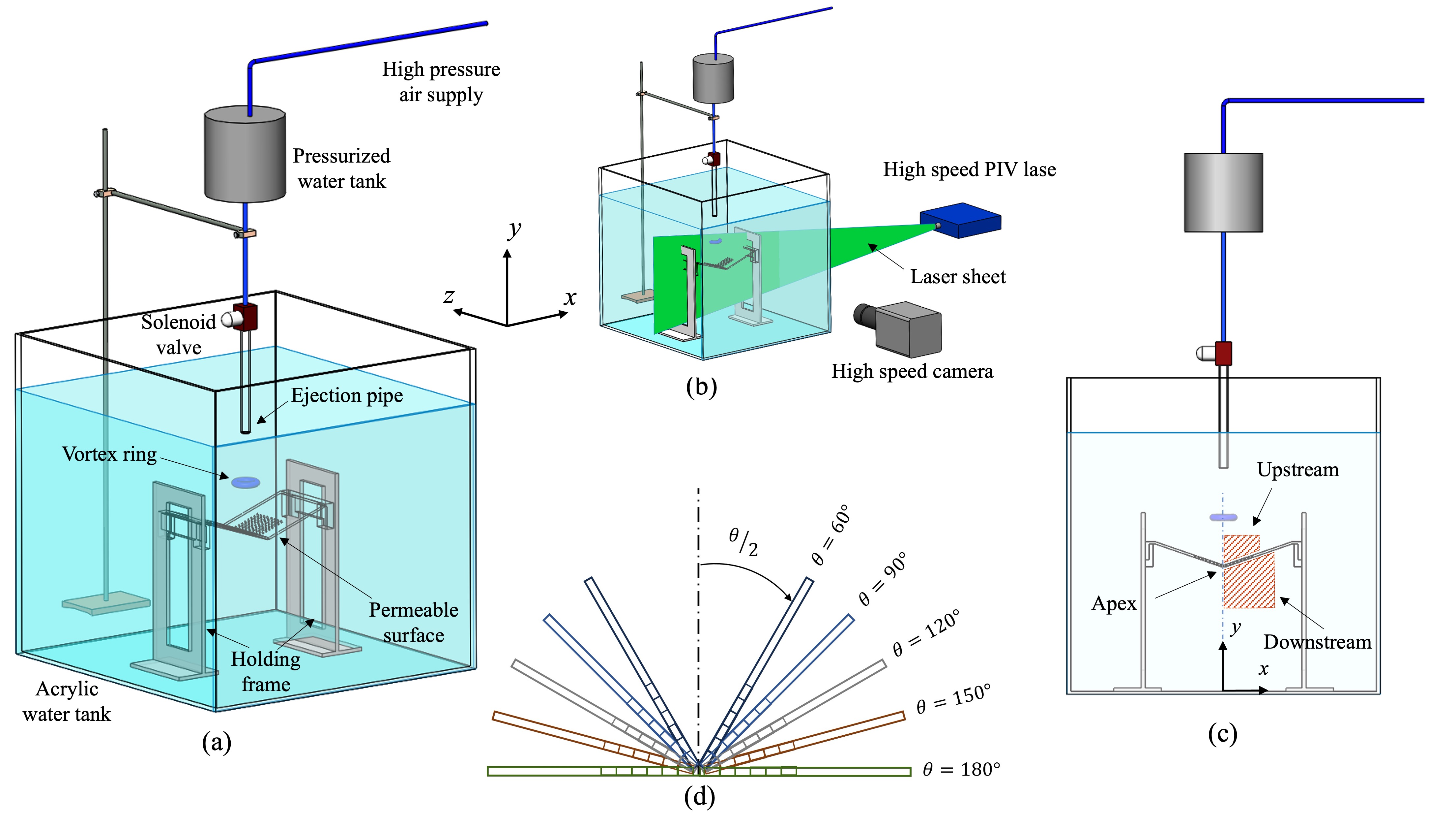
Figure 1: (a) A 3-dimensional view of the experimental setup (b) Setup for PIV and PLIF measurements (c) A 2-dimensional view of the experimental setup. The hatched zone shows qualitatively the area considered for calculation of the circulation using the PIV data (d) Different configurations of the perforated surface used in the present study.

2.2 PIV and PLIF

The PIV measurements were done using a high-speed dual pulse Nd:YLF laser (Photonics Inc.,pulse energy of 30 mJ, emission wavelength 527 nm). Both PIV and PLIF recordings were done at 1000 Hz. A typical setup for both PIV and PLIF experiments are shown in figure 1(b). For uniform illumination of the interaction zone, cylindrical lens beam was expanded and converted into a planar sheet of thickness $\sim$ 1 mm. Neutrally buoyant borosilicate glass spheres (Signma-Aldrich) of mean diameter ranging from 9-13 ${\mu}$m and having density of 1100 Kg m^-3 were dispersed in water homogeneously and were illuminated by laser sheet. The seeder particles were also mixed with the water that was used to generate the vortex ring along with the quiescent fluid in the tank. The laser entered the acrylic tank from one side (figure 1(b)) that was aligned precisely with the array of holes to acquire accurate flow field data coming out of the hole. The images were recorded using Photron Mini UX high-speed camera at a pixel resolution of 1280 pixels x 1024 pixels with a field of view of $\sim$ 66 mm x 53 mm. Cross-correlation technique with constant multi-pass interrogation window size of 64 pixels x 64 pixels was employed to process the displacement vectors. 75% overlap was fixed for all the cases resulting in vectors at spacing of 0.84 mm. The captured PIV images were post-processed in Davis 8.4 software to obtain the velocity and vorticity fields that is subsequently utilized to construct FTLE fields and locate vortex cores using $\Gamma_{2}$ method.

Additionally, for PLIF experiments a small amount of rhodamine 6G dye was mixed with the fluid used to generate the vortex ring and the emitted light was captured using the same camera mentioned above at 1000 Hz. A band-pass filter of 570 ± 10 nm (suitable for the emission range of fluorescent dye) was attached in front of the camera lens (LaVision) to block the scattered and stray light from entering the camera sensor.

2.3 Lagrangian coherent structures (LCS) using FTLE

In the present work, the finite-time Lyapunov exponents (FTLE) analysis is used to extract the LCS to study the interaction and mixing of the emerging jets from the perforated surface on interaction with vortex ring. The FTLE fields are directly calculated using the velcoity field obtained from the PIV data. FTLE is a scalar field that is used to measure at each point in space, the rate of separation of neighbouring particle trajectories initialized near that point (Haller, 2001). The method gained popularity in the last decade and is well documented (Haller, 2000; Shadden et al., 2005; Haller, 2015). Under the action of a flow map ${F_{t_{0}}^{t_{f}}}$ the fluid particle x(${t_{0}}$) and x(${t_{0}}$)+ ${\delta}$(x(${t_{0}}$)) are defined in space and time. Using the local spatial gradients in the flow map i.e., ${\nabla}$${F_{t_{0}}^{t_{f}}}$(${x_{0}}$), the Cauchy-Green tensor is constructed (Haller & Sapsis, 2011). The coefficient of expansion or the measure of strain is then defined as

$$\sigma(x_{0},t_{0})={\lambda_{max}}([\nabla{F_{t_{0}}^{t_{f}}}({x_{0}})]^{\otimes}[\nabla{F_{t_{0}}^{t_{f}}}({x_{0}})])$$ (1)

where $\otimes$ refers to the transpose of the matrix and $\lambda_{max}$ refers to the largest eigenvalue. The FTLE field is then defined as

$$FTLE(x_{0},t_{0})=\frac{1}{T}\log{\sigma({x_{0},t_{0}})}$$ (2)

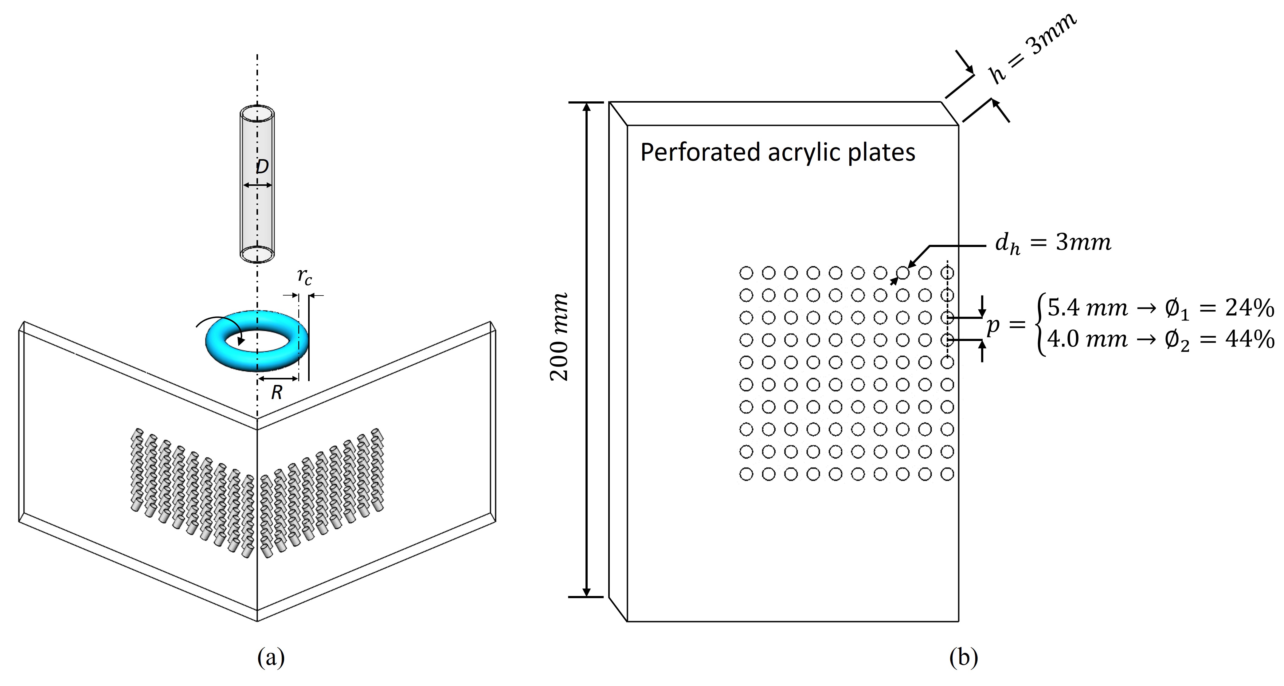
Figure 2: (a)A 3-dimensional schematic depicting various parameters of the vortex ring and ejection pipe (b) Dimensions of the two perforated surfaces used in the present study

(For more details see (Shadden et al., 2005)). The maximum values of FTLE corresponds to the LCS in the flow field. We calculate the FTLE in reverse time known as the backward FTLE that is associated with the convergence of the fluid particles. Higher values of FTLE means higher degree of convergence. The integration time T can be chosen based on the extent the LCS needs to be captured (Shadden et al., 2007) however the trajectories should not leave the velocity field domain. We choose different values of T for different frame cautiously keeping a check on the particle not getting accumulated at the perforated surface and not leaving the flow domain. Further, the value of T should not be kept smaller than the time scales of the formation of the coherent structures. Finer spatial grids results in better and sharper fields (Vetel et al., 2009; Espa et al., 2012). In the present work, the grid resolution was increased to obtain sharper LCS ridges. The FTLE ridges can be successfully utilized to identify boundaries of the coherent structure in both laminar or turbulent flows like oceanic flows (Olascoaga et al., 2013), large scale environmental flows (Olascoaga & Haller, 2012), mixing in turbulent flows (Mathur et al., 2007), laminar flow structures like periodic shedding of vortices behind bluff bodies (Kasten et al., 2010), vortex ring formation in heart (Espa et al., 2012) and more (Haller, 2015).

2.4 ${\Gamma_{2}}$ method for vortex core identification

The use of vorticity fields to detect vortices can lead to erroneous interpretations (Hussain & Jeong, 1995). Since, vorticity calculation involves velocity gradients, the vorticity fields can fail to differentiate between shear layers and rotating regions. In the present work, we use vorticity contours to calculate the circulation and ${\Gamma_{2}}$ method to educe the centres of rotating vortices. ${\Gamma_{2}}$ method, as proposed by Graftieaux et al. (2001) is defined as

$$\Gamma_{2}(P)=\frac{1}{N}\sum_{S}\frac{({\vec{PQ}}\times({\vec{U_{Q}}-\vec{U_{m}}}))\cdot\vec{z}}{\parallel\vec{PQ}\parallel\cdot\parallel\vec{U_{Q}}-\vec{U_{m}}\parallel}$$ (3)

where the formulation is applied at each point P in the vector field obtained from the PIV data to find the normalized scalar $\Gamma_{2}$ values. $\vec{PQ}$ denotes the displacement vector from point P to Q inside area S, $\vec{U_{m}}$ refers to the mean velocity of the area S, $\vec{U_{Q}}$ refers to the velocity vector at point Q and $\vec{z}$ is the unit vector perpendicular to the plane. The threshold for the vortex centre is considered to be 0.75 (i.e., $>$ 2/$\pi$) since the structures form in the downstream region after interaction are turbulent and chaotic in nature. The consideration of the local velocity vector $\vec{U_{m}}$ makes the method Galilean invariant unlike $\Gamma_{1}$ method (Graftieaux et al., 2001).

Pin	rc	R	Uc	${\Gamma_{0}}$	ReΓ	Reconv
(psi)	(cm)	(cm)	(cm/s)	($cm^{2}/s$)	(${\Gamma_{0}/\nu}$)	(${U_{c}R/\nu}$)
40	0.36 $\pm$ 1%	0.8 $\pm$ 1.6%	30 $\pm$ 3%	115 $\pm$ 1.1%	11500	2400

Table 1: Different parameters of the vortex ring. The $\pm$ % indicates the positive and negative standard deviation values of the corresponding mean values. Here, P_in refers to the injection pressure at which the vortex ring is generated inside the water; r_c refers to the radius of the core of the vortex ring (check figure 2(a)); R is the distance between the vortex centre to the core known as the radius of the vortex ring (check figure 2(a)); U_c is the convection velocity of the vortex core in y direction calculated by tracking the vortex core; ${\Gamma_{0}}$ is the circulation of the free vortex ring i.e., the case without any perforated plate; Re_Γ is Reynolds number based on circulation; Re_conv is the Reynolds number based on convection velocity and ring radius.

2.5 Experimental conditions and measurements

The experiments are conducted under water at room temperature. For all the values of ${\phi}$ and ${\theta}$ the distance between the ejection pipe and the apex of the perforated surface was kept at 7D. This distance is kept such that the vortex ring is fully developed during the start of the interaction. It is worth noting that in the present scenario, at lower ${\theta}$, the vortex ring will start interacting earlier compared to larger ${\theta}$ values and hence the apex is considered as the reference point from which the y axis passes. This axis also coincides with the translational axis of the vortex ring. The various specifics of the vortex ring are enumerated in Table 1 and has been depicted in Figure 2(a). The velocity and vorticity (${\omega}$) fields obtained from the PIV measurements are used to calculate the circulation (${\Gamma}$) by taking the area integral of the vorticity field. The formulation for circulation is given as

$$\Gamma=\int_{C}\omega dA$$ (4)

where C is the area of interest. For all the cases, a threshold of 10% of the maximum vorticity was considered to calculate the circulation which was found to be sufficient to eliminate the background noise in the PIV data. For calculating the circulation, a masking region was defined as shown in Figure 1(c) encompassing the desired events.

3 Results and Discussion

3.1 Characterization of the vortex ring

Vortex ring having Re_Γ = 11500 (at 5D from ejection pipe) is considered in the present study to understand how ${\theta}$ and ${\phi}$ influences the interaction. Figure 3(a) depicts the variation of ${\Gamma^{+}_{0}}$ and ${\Gamma^{-}_{0}}$ (circulation generated by positive and negative vorticity respectively) of the free vortex ring (without perforated surface) with T^∗ (non-dimensionalised using the ratio ${U_{c}/D}$). This period corresponds to a physical distance of $\sim$ 3 cm (2.5D) starting at 5D from the ejection site. The constant value of circulation confirms the fully developed condition of the vortex ring before the interaction. Figure 3(b) shows the y velocity profile of the vortex ring along the line joining the two cores as shown in the inset. The profile obtained corresponds to a typical velocity profile across the vortex ring (Maxworthy, 1977). From the profile, the symmetric nature of the vortex ring can be confirmed. Figure 3(c) depicts the velocity vector field of a propelling vortex ring superimposed over the vorticity contours. The centres of the two cores are identified using the $\Gamma_{2}$ method as described in section 2.4. It is clear that the peak vorticity and the centre do not coincide. The backward time FTLE field of the vortex ring is laid over the vector field in figure 3(d). The bright ridges corresponding to the higher FTLE values demarcating the vortex ring boundary across which material transport remains restricted.

Figure 3: (a) Variation in positive and negative circulation of the free vortex with the non-dimensional time (${T^{*}=\textit{${U_{c}/D}$}}$). The distance covered during this time period is starts from 5D till 7.5D from the ejection pipe (b) The y-velocity ($V_{y}$) profile of a free vortex at 5D distance form the ejection pipe along the line passing through the vortex core as shown in the inset (c) Vorticity contour plot of a free vortex ring overlaid over velocity vectors field. The pink and green dot represents the counter-clockwise (CCW) and clockwise (CW) vortex core detected using $\Gamma_{2}$ method (d) The backward FTLE field of a free vortex overlaid over the velocity vector field.

3.2 Qualitative aspects of the interaction

To develop an initial understanding of the interaction, we show in figure 4 and 5 the time sequenced PLIF images at different non-dimensional times (T^∗= ${tU_{c}/D}$)) for all the ${\theta}$ values at ${\phi_{1}=0.24}$ and ${\phi_{2}=0.44}$. T^∗= 0 is consider just before the dyed vortex collides with the perforated wall. Due to hindrance from the perforated surface, the left side of the interaction process is not visible or partly visible hence, the right side is considered for discussion. An important aspect of increasing the ${\theta}$ values is that it delays the interaction phenomenon and shifts the interaction site further downward. This combined with the ${\phi}$ has a direct consequence on the number of holes involved during the interaction process. For ${\phi_{1}\theta^{60}}$ (Figure 4), the vortex ring on interaction starts emerging out as unstable jets from the $4^{th}$ hole counted from the apex. This number decreases by 1 till ${\phi_{1}\theta^{120}}$ after which it emerges from 2 holes. For $\phi_{2}$, the number of holes remain 5 for ${\phi_{2}\theta^{60}}$ that decreases by 1 till ${\phi_{1}\theta^{150}}$. This is because of smaller pitch between holes for ${\phi_{2}}$ compared to ${\phi_{1}}$ (check figure 2). These observations will be quantitatively explained in further sections. For both ${\phi_{1}\theta^{180}}$ and ${\phi_{2}\theta^{180}}$ the vortex ring comes out of 5 holes however, shifting the position of the perforated surface for ${\phi_{2}\theta^{180}}$ results in involvement of 6 holes. For consistency, we ignore this case in the present study and consider the case when the translational axis of the vortex ring coincides with one of the hole centres for ${\phi_{2}\theta^{180}}$.

Figure 4: The PLIF images for ${\phi_{1}}$ at ${\theta}$ = 60° - 180° shown at different ${T^{*}}$. The scale represents 5 mm.

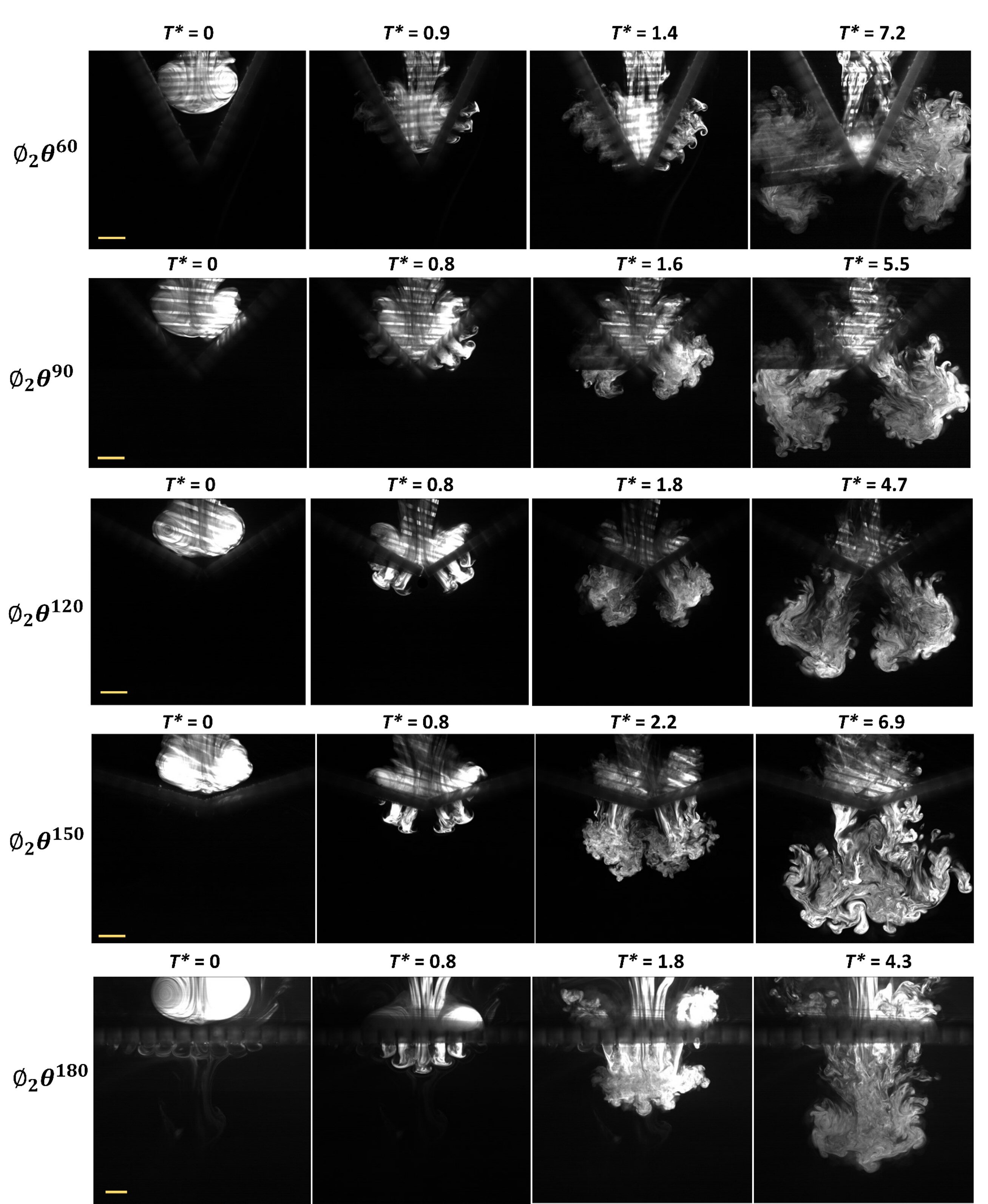
Figure 5: The PLIF images for ${\phi_{2}}$ at ${\theta}$ = 60° - 180° shown at different ${T^{*}}$. The scale represents 5 mm.

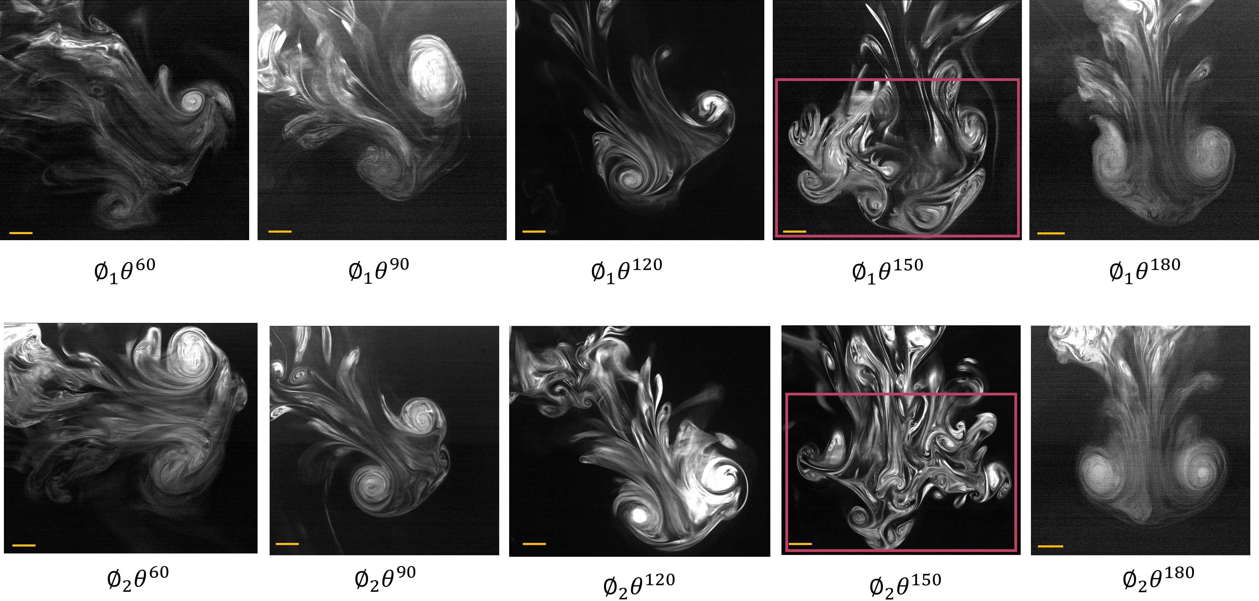
Figure 6: The reformation of the vortex ring in the far downstream region ($\sim$ 6D from the apex). The red box in case of $\theta$=150° depicts the suppression of the reformed vortex ring. The scale bars represents 5 mm.

On interacting, the vortex ring breaks down into circular jets that develop instability over very small time scales. Due to the quiescent nature of fluid downstream of the surface, Kelvin-Helmholtz (K-H) instabilities grows at the shear layers of the jets that are clearly visible in the figures (4-5). For cases with lowest $\theta$ value (i.e., 60^∘), the flow after interaction has a high tendency to curl in the same sense as the right hand part of the vortex ring (as will be discussed in section 3.3.2, check figure 14). The emerging jets starts travelling in x direction with their heads rotating in an opposite sense. This can be clearly seen in ${\phi_{2}\theta^{60}}$ (Figure 5) where the head of the jets roll up to form series of circular pattern, a feature very commonly observed during the occurrence of K-H instabilities. Furthermore, for ${\phi_{1}}$ the out-coming jets maintain a distance with the adjacent jets for a long time before interacting as is visible in Figure 4 (${\phi_{1}\theta^{60}}$ : T^∗=1.1, ${\phi_{1}\theta^{90}}$:T^∗=1.3, 1.6, ${\phi_{1}\theta^{120}}$:T^∗ = 0.8, ${\phi_{1}\theta^{150}}$: T^∗=1.1, 1.7, ${\phi_{1}\theta^{180}}$: T^∗=1). Whereas in cases with ${\phi_{2}}$, these jets interacts with their adjacent jets very early because of the proximity of the holes. These early interactions makes the downstream flow highly chaotic in nature. Adding on to the instabilities, we observe an intriguing phenomenon that results in the mushroom shaped features at the head of the jets that will be discussed in section 3.2.1.

The jets after ejecting out self interacts resulting in a violent mixing of the fluid that has been observed in previous studies (Xu et al., 2018; Jain et al., 2023). This interaction is characterized by 3-dimensional mixing and vorticity cancellation. The consequence of vorticity cancellation is the formation of two primary coherent structures in the downstream with low strength . With increasing ${\theta}$, the fluid from the two halves of the surface starts to approach each other and interacts for ${\theta}$=150° (figures 4 and 5, $\theta$=150°). The distance at which the two halves interact is not sufficient for each half to form the downstream vortex hence, we did not observe collision of two downstream regenerated vortex. Due to this type of interaction, no coherent structure is observed for ${\phi_{1}\theta^{150}}$ cases. For all the other cases the regenerated downstream vortex is shown in Figure 6.

It can be understood that on interaction, the vortex ring expands in the z direction as well as has been discussed by New et al. (2020) in details. In their study, the walls had no penetration condition which forced the vortex ring to expand in the z direction. In the present study due to the change in the penetration condition at the wall, we see a rapid passage of vortex core through the holes in a sequential manner as discussed above. An image (see supplementary figure S1) has been provided to illustrate the amount of dyed fluid ejecting of the holes present in the z direction from the apex for ${\phi_{1}\theta^{90}}$. The image shows that for lower open area ratio i.e., ${\phi_{1}}$, the amount of fluid coming out at different distances remains significantly less. Essentially, this must depend strongly on the ${\phi}$ value of the system and is expected to be much more lesser for ${\phi_{2}}$.

3.2.1 Initial instability on jets

It is well known that vortex ring induces fluid motion around themselves. The velocity field around a vortex decreases gradually as shown in figure S2 and the induced velocity field around the perforated surface for $\theta$ = 60° is shown in figure S3. Due to the induced flow and the presence of perforated surface of appreciable thickness, the fluid ahead of the vortex ring crosses the perforated surface much before the vortex ring does. As the induced flow passes through the holes, the shear resistance offered by the holes leads to the development of mushroom shape front. This can be seen in figures 7 and S4 where we capture this phenomenon for ${\theta}$ = 150°  and 180° respectively by pouring a thin layer of rhodamine dye over the perforated surface just before the vortex ring approaches it. This front is further caught up by the main flow from the vortex which can be seen from the marked images (figures 7 and S4). The initial jets have low kinetic energy as the peak comes later (T^∗ $>$ 1, check figure 8) due to penetration of the core and hence this initial jet converges to the shape of this mushroom. This imparts the initial instability to the jet heads and they form a mushroom shaped feature.In case of ${\phi_{2}}$, these mushrooms remains at close proximity tending to overlap at the edges thereby forming a continuous structure (figure 7(b) and S4), unlike in ${\phi_{1}}$ where the boundaries of the mushrooms are distinctly detectable. As the core starts to penetrate, velocity peak is obtained and intense mixing between jets is observed along with K-H instability at the edges of the jets. The initial instability discussed here adds on to the rolling up of the jets at their heads. This type of mushroom formation is a direct consequence of placing a perforated plate with considerable thickness in the path of a vortex ring.

3.3 Quantitative aspects of the interaction

3.3.1 Evolution of velocity and vorticity field near the surface

As seen in the preceding sections, the vortex ring on colliding with the inclined perforated surface emerges out in a sequential manner. To better understand the phenomenon we plot the non-dimensional velocity magnitude (${V_{mag}^{*}}$, normalised using the velocity magnitude of the free vortex) and the dimensional vorticity values about a line at a distance of $\sim$ 0.5D from the perforated surface in the downstream region as shown in figure 8 and 9 respectively. This distance was considered to avoid the contamination of the data by the noisy signals generated near the wall. Also, beyond this distance, some of the peaks were lost for few cases. In the y axis the non-dimensional length ($L^{*}=L/D$) with 0 being the apex point is plotted along with the non-dimensional time ($T^{*}=tU_{c}/D$) in the x axis. $T^{*}=0$ is considered the frame just before the velocity vectors starts emerging from the perforated surface in the PIV data. The primary purpose of these plots is to depict the sequential generation of jets form the perforated plate and to capture the near wall events when the jets emerge out. For ${\phi_{1}\theta^{60}}$, we see a weak $V_{mag}^{*}$ peak followed by three dominant peaks occurring one after the other as time progresses (figure 8). Although for ${\phi_{1}\theta^{60}}$ the vortex interacts early with the wall, the initial impact remains weak and vortex rapidly gets sucked in towards the apex. The initial interaction does not involve the disintegration of the vortex core resulting in a feeble peak. Overall, we see three major peaks for this case that slowly convects out with time. Similarly for ${\phi_{2}\theta^{60}}$, the interaction starts even earlier which is expected and 5 distributed peaks are obtained in a successive manner (figure 8). The phenomenon seen in the PLIF images (figure 4 and 5) for ${\theta}$=60° has been beautifully captured by the PIV data as can be seen form the vorticity values plotted in figure 9. For ${\phi_{1}\theta^{60}}$ we can see the appearance of alternate sense of vorticity patches i.e., positive vorticity (red contours, CCW) sandwiched between negative vorticity zones starting from the farthest hole with weak negative vorticity zone. Whereas for ${\phi_{2}\theta^{60}}$, we can see a continuous stretch of CW vortices appearing initially followed by slightly shifted stretch of CCW vortices. The vorticity zone near the apex maintains its vorticity for the longest period due to the decay of the vortex near apex.

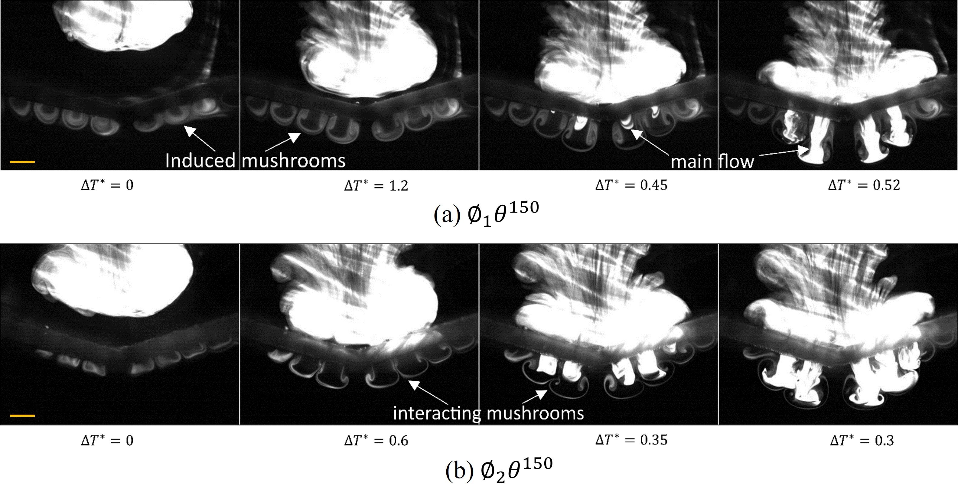
Figure 7: The PLIF images for ${\phi_{1}\theta^{150}}$ and ${\phi_{2}\theta^{150}}$ depicting the initial jet instability due to mushroom formation. Here, $\Delta T^{*}$ is the difference in $T^{*}$ The scale represents 5 mm.

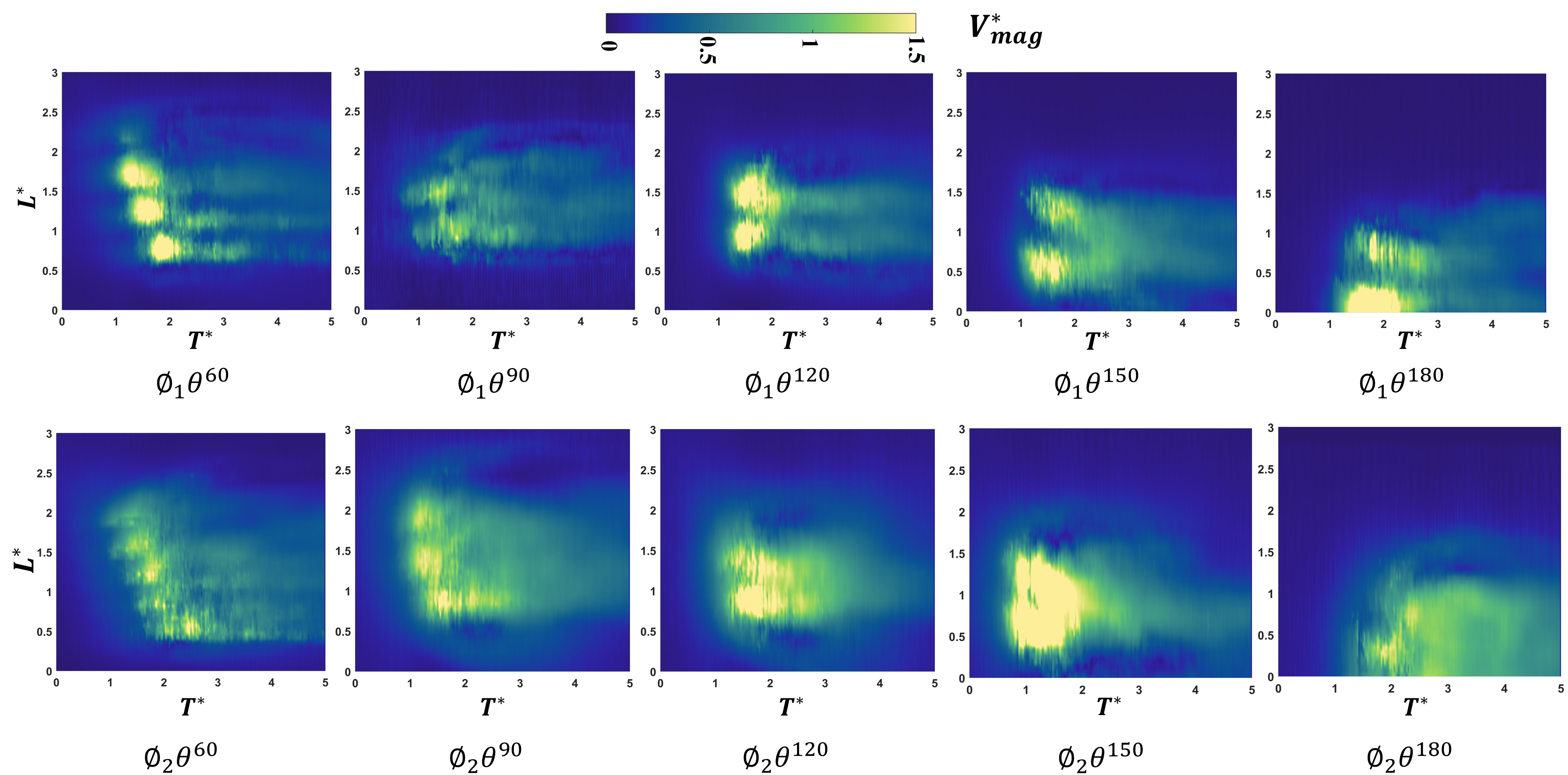
Figure 8: The non-dimensional velocity magnitude (non-dimensionalised using free vortex ring velocity magnitude) contour plotted against ${T^{*}}$ and ${L^{*}}$ (= $L/D$ where L is the length of the line about which the data is plotted) at a distance of 0.5D from the perforated surface.

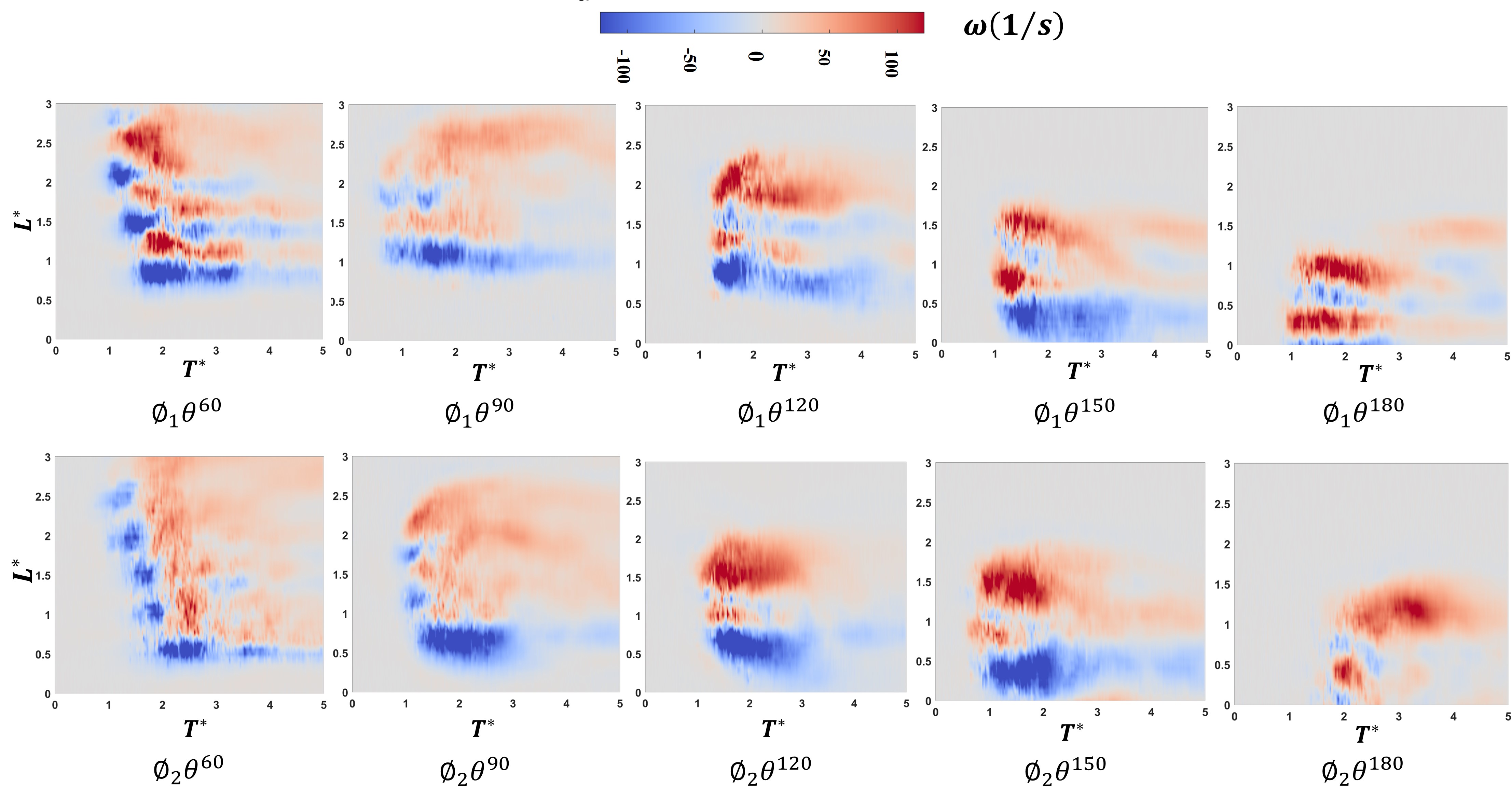
Figure 9: The dimensional vorticity contour plotted against ${T^{*}}$ and ${L^{*}}$ (= $L/D$ where L is the length of the line about which the data is plotted) at a distance of 0.5D from the perforated surface.

For ${\theta}$ = 90°, three velocity peaks are seen followed by two peaks for the rest of the cases (figure 8). For cases with ${\phi_{1}}$, a distinct gap between the peaks can be observed that is not present in case of ${\phi_{2}}$. For ${\phi_{2}\theta^{150}}$, the peaks are seen to be merging with each other. Another important information that can be extracted from the plot is that for ${\theta}$ $\geq$ 120° , the first velocity peak occurs nearer to the apex and the second peak occurs away from it i.e., there is reversal in the sequence in which the jets come out (figure 8). This suggest that the core first starts to penetrate from the holes nearer to the apex of the perforated surface. Hence, for the present set of parameters, ${\theta}$ = 120° behaves like a transition point where the flow field changes and starts to tend towards $\theta$ = 180°. Moreover with increase in ${\theta}$, the overall flow map (figure 8 and 9) can be seen to be shifting towards $L^{*}$ = 0. For ${\phi_{2}}$, the vorticity zones are more circular in shape compared to ${\phi_{1}}$ where they are more linear. The overall vorticity dynamics will be discussed in the next section.

3.3.2 Vorticity dynamics

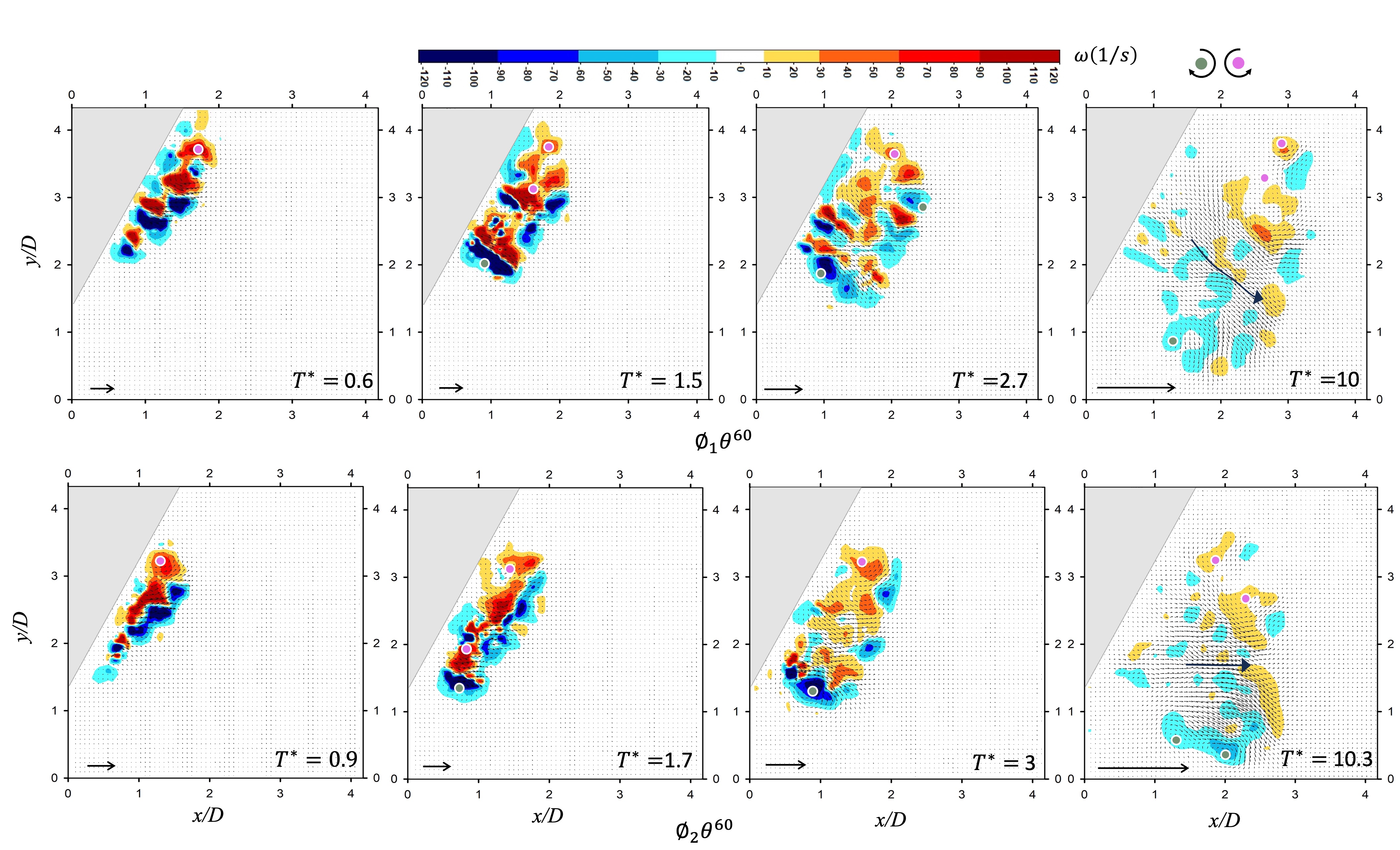
Figure 10: Evolution of vorticity field for ${\phi_{1}\theta^{60}}$ and ${\phi_{2}\theta^{60}}$ plotted at different $T^{*}$ values. The scale vector indicates $1m/s$. The pink dot represents the CCW rotating vortex cores and the green dots represents the CW rotating vortex cores detected using $\Gamma_{2}$ method.

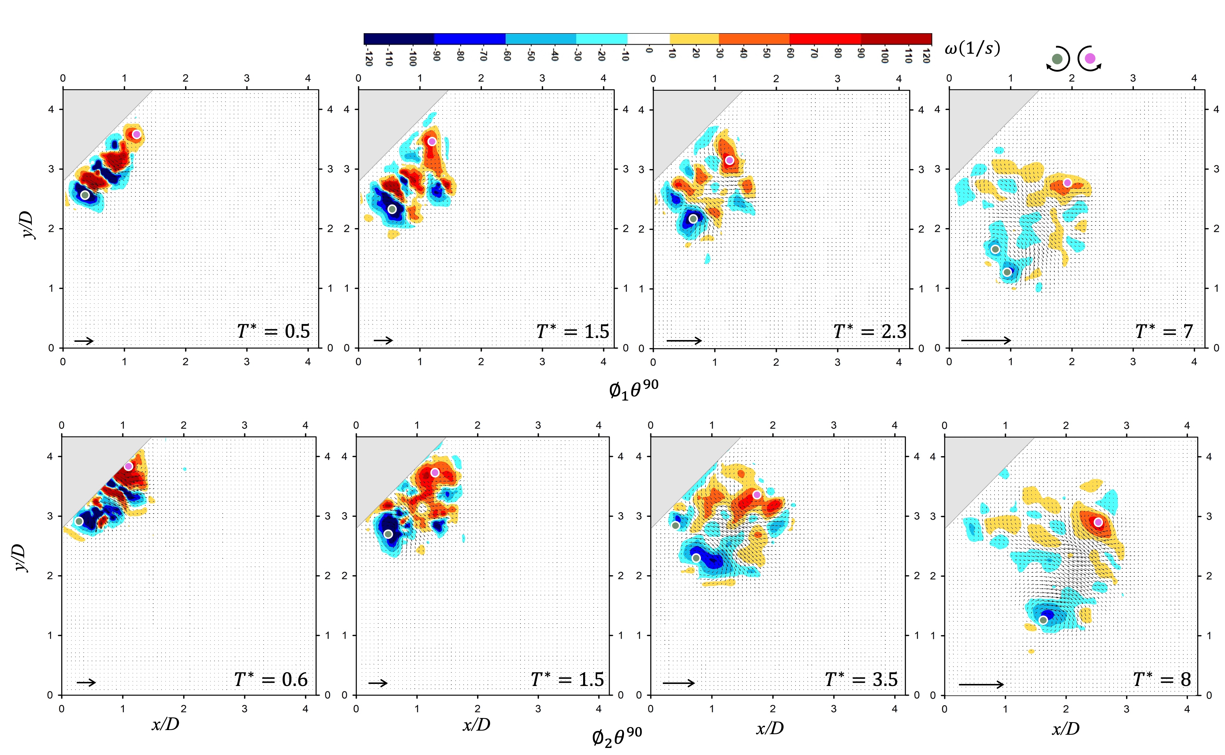
Figure 11: Evolution of vorticity field for ${\phi_{1}\theta^{90}}$ and ${\phi_{2}\theta^{90}}$ plotted at different $T^{*}$ values. The scale vector indicates $1m/s$. The pink dot represents the CCW rotating vortex cores and the green dots represents the CW rotating vortex cores detected using $\Gamma_{2}$ method.

We plot the vorticity contours over the vector fields obtained from the PIV data in figures 10-14 for different ${\theta}$ values in the increasing order. When a vortex ring interacts with a perforated plate of such kind, the emerging flow in the downstream remains highly chaotic. The reason for this being the conversion of the vortex core to single jets and their further interaction with each other. For cases with ${\theta}$ $\leq$ 120° , we see this phenomenon occurring symmetrically on two halves of the surface whereas for ${\theta}$ $>$ 120 the jets on both sides starts talking to each other. These features will be highlighted in this section where we discuss how the vortex cores move and interact in the downstream region. We denote the clockwise (CW) and counter (CCW) rotation of vortices by their centre using green and pink dots respectively. The location of the dots have been identified using the $\Gamma_{2}$ method as described in section 2.4.

Figure 12: Evolution of vorticity field for ${\phi_{1}\theta^{120}}$ and ${\phi_{2}\theta^{120}}$ plotted at different $T^{*}$ values. The scale vector indicates $1m/s$. The pink dot represents the CCW rotating vortex cores and the green dots represents the CW rotating vortex cores detected using $\Gamma_{2}$ method.

For ${\phi_{2}\theta^{60}}$ we see a stretch of negative vorticity coming out of the surface compared to ${\phi_{1}\theta^{60}}$ where the features resembles more like individual jets (figure 10). A CCW vortex develops near the hole that is farthest to the apex. The vorticity remains more distributed in case of ${\phi_{2}\theta^{60}}$ and the flow moves at a slower speed. For ${\phi_{1}\theta^{60}}$ ultimately the flow converges to the development of two major vortical regions that propel in the direction nearly perpendicular to the perforated surface. For ${\phi_{2}\theta^{60}}$, the CW vortex that develops near the apex has more vorticity and propels faster than the CCW resulting in the horizontal convection of the flow. The faster motion of this CW vortex is a result of the final momentum that is is imparted by the disintegration of the core near the apex. The two vortical regions at the extreme ends of the flow is seen to break up into multiple small scale vortical zones. Similar is the case for ${\theta}$ = 90°(figure 11) where the rotating zones develop very early and propels in a nearly normal direction.

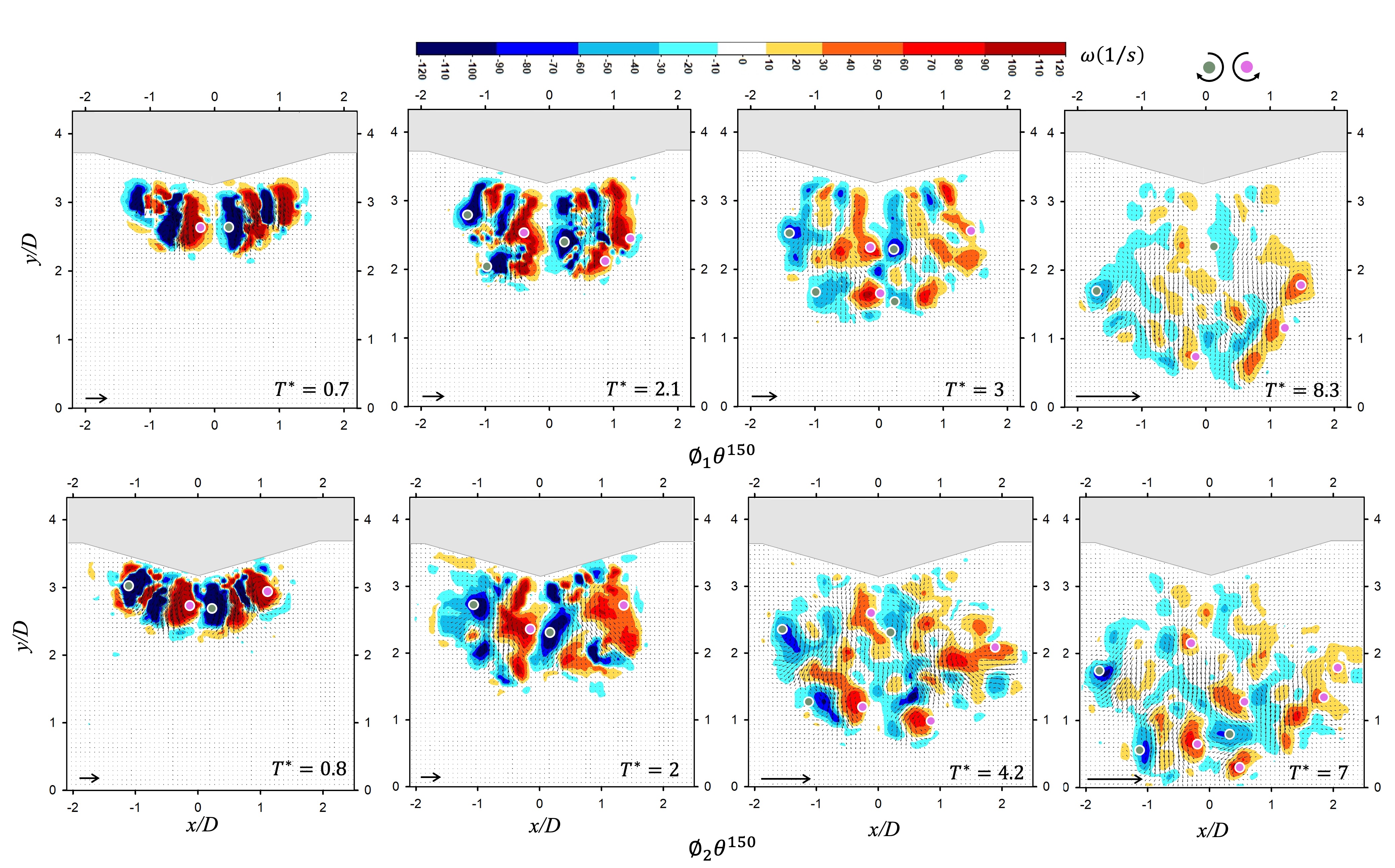
Figure 13: Evolution of vorticity field for ${\phi_{1}\theta^{150}}$ and ${\phi_{2}\theta^{150}}$ plotted at different $T^{*}$ values. The scale vector indicates $1m/s$. The pink dot represents the CCW rotating vortex cores and the green dots represents the CW rotating vortex cores detected using $\Gamma_{2}$ method.

We depict both the sides of the flow for ${\theta}$ $\geq$ 120°to identify the $\theta$ at which the flow on the two halves starts to interact with each other. Jets of opposite vorticity can be seen to develop initially around $T^{*}$ = 0.65 for ${\phi_{1}\theta^{120}}$ with the rotating regions on the outer and inner sides of the flow on each side (figure 12). For ${\phi_{2}\theta^{120}}$ instead of long jets, we see circular patches of vorticity developing initially around the same time. The out coming flow in ${\phi_{2}}$ already starts to interact due to the proximity of the holes resulting in larger circular patches. Interestingly, the vorticity cancellation process seems less intense in these larger vorticity zones (in ${\phi_{2}}$) compared to the jets (in ${\phi_{1}}$) resulting in the higher vorticity values of the core at a later instance. Due to a larger spreading area in case of ${\phi_{2}\theta^{120}}$, we can see at ${T^{*}}$ = 3.4, the inner vortical cores come very near to each other ultimately diverging in the flow direction.

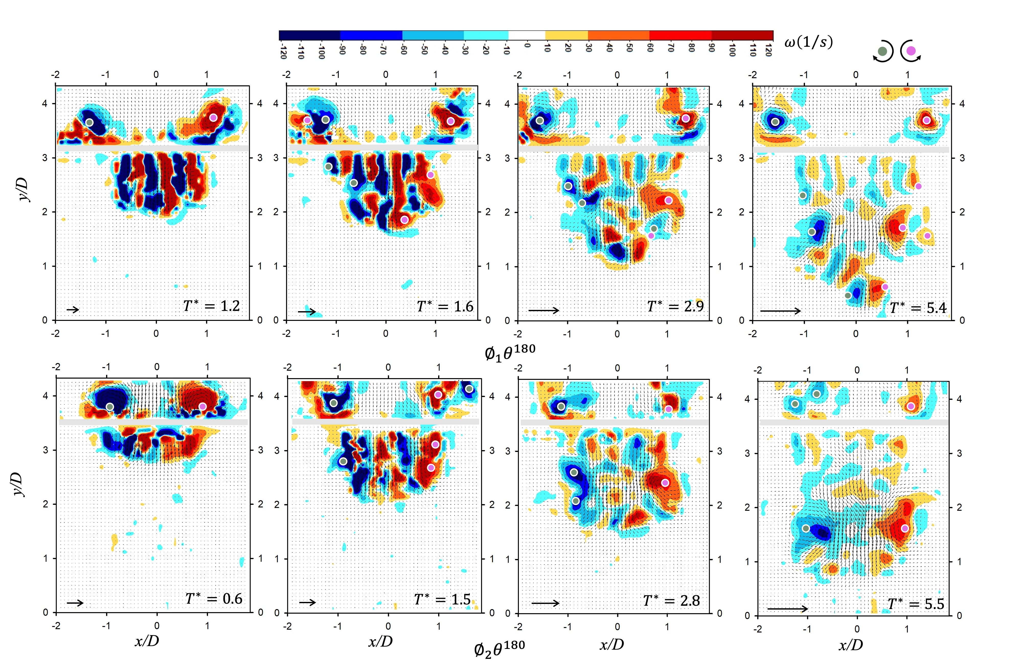
Figure 14: Evolution of vorticity field for ${\phi_{1}\theta^{180}}$ and ${\phi_{2}\theta^{180}}$ plotted at different $T^{*}$ values. The scale vector indicates $1m/s$. The pink dot represents the CCW rotating vortex cores and the green dots represents the CW rotating vortex cores detected using $\Gamma_{2}$ method.

For cases with ${\theta}$ = 150°(figure 13), the flow initially behaves similarly to the preceding case with much more proximity between the inner jets from other halves. Along with vorticity cancellation on each sides of the surface, we see clear interaction of the vortex cores for ${\phi_{1}\theta^{150}}$ at ${T^{*}}$ = 3 and ${\phi_{2}\theta^{150}}$ at ${T^{*}}$ = 2. Neat jets of fluid can be discerned for ${\phi_{1}\theta^{150}}$ that results in vorticity cancellation from adjacent jets and ultimately breaks into multiple vortical zones as shown in figure 13. However, a less coherent flow is observed for ${\phi_{2}\theta^{150}}$ resulting in the development of many vortical zones resembling turbulent flows. As shown in figure 6 (red marked zone), the vortex reformation in the far downstream does not happen in case of ${\theta}$ = 150° due to the interaction of flow from other halves.

For ${\theta}$ = 180°(figure 14) we show both the upstream and the downstream regions of the perforated surface. For other cases the upstream flow was not depicted because of the uncertainty in the PIV data that can arise in cases with lower ${\theta}$ values due to wall effects. In this regard, a discussion and plot (figure S5) is presented in the supplementary sheet that shows the effect of $\phi$ and $\theta$ on the circulation of the vortex ring just before the interaction. On the upstream side, as the vortex approaches the surface boundary layer of opposite sense starts to develop that separates to form the secondary vortices of opposite sense (Naaktgeboren et al., 2012; Jain et al., 2023). It can also be seen that the vortex core sustains for a longer period in case of $\phi_{1}$ which is expected due to lesser porosity. For ${\phi_{1}\theta^{180}}$, the jets of opposite vorticity interact and shed vortices from the head in the central region as can be seen in figure 14. The central vortical structure is a result of the vorticity cancellation and the unstable head of the jets due to the initial mushroom type instability as discussed in section 3.2.1. These central vortices are also seen for ${\phi_{1}\theta^{150}}$ at ${T^{*}}$ = 3 due to the interaction of the central jets and their shedding. Along with theses small structures, the overall flow preserves the axial bulk velocity at the central region resulting in the formation of two large vortical cores at the edges of the flow field (Jain et al., 2023). In contrast, we do not observe central vortices for ${\phi_{2}\theta^{180}}$ and two large scale vortical structures form after the central vortices cancel each other.

A quantitative comparison of the non-dimensional circulation generated by the positive and negative vorticity in the downstream region is presented in figure 15 for each of the cases. Owing to symmetry, we consider the right side of the apex axis for all the cases (as shown in figure 1(c)). The pink line depicts the circulation generated by the positive vorticity ($\Gamma^{+}$, CCW) and the green line shows the circulation generated by the negative vorticity ($\Gamma^{-}$ ,CW). Since the right hand side of the flow is considered, the side of the vortex ring having CCW sense about the XY plane is discussed. The fluid emerging out innately has a natural tendency to generate positive circulation in CCW direction. This is observed in all the cases with the pink line always having higher value compared to the green line. In figure 15, for $\theta$=180° as well the right hand side of the flow is considered. Figure S6 has been provided having the positive and negative circulation for the whole field depicting the symmetricity of the interaction process. For $\theta$ = 60° initially, the flow is highly dominated by the positive vorticity in (especially ${\phi_{2}\theta^{60}}$) which further subsides to constant values. The trend in case of $\theta$ = 90° and $\theta$ = 120° almost remains similar. It can be inferred from the graph that the ratio of positive circulation to the absolute of negative circulation for $\theta$$\leq$ 120° becomes constant (near $\sim$ 1) after a point of time indicating the development of two coherent vortex structures of similar circulation without any further generation of circulation. Interestingly, for $\theta$ = 120° the pink and green line remains very near and behaves similar to what is shown in figure S6 for the full flow field of $\theta$ = 180° . Further, the difference between the peaks goes on decreasing till $\theta$ = 150° where we see the peaks of around similar strength coming out of the one side of the surface. However, intriguingly we observe that the green and pink line does not converge any more as seen in cases below $\theta$ $\leq$ 120° .

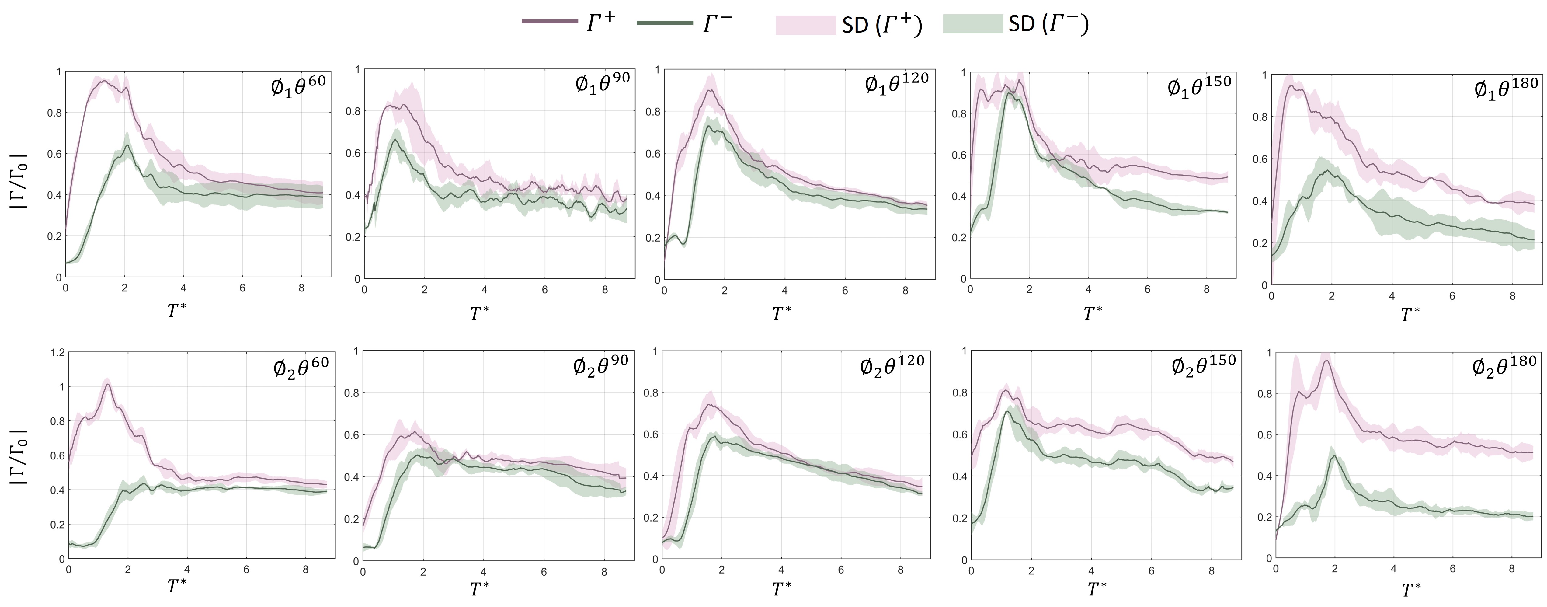
Figure 15: The variation of absolute values of non-dimensional positive and negative circulation (non-dimensionalised by $\Gamma_{0}$ for each case) in the downstream region of the flow field after interaction for all the cases with $T^{*}$. Here, $T^{*}$ = 0 represents the instance at which the velocity vectors becomes detectable after interaction in the downstream region. SD represents standard deviation of the data.

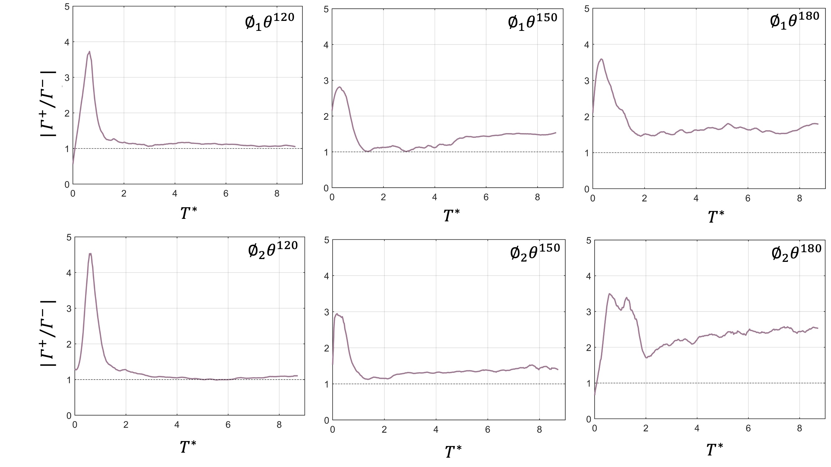
Figure 16: The variation of the ratio of absolute values of positive and negative circulation in the downstream region of the flow field after interaction for the mentioned cases with ${T^{*}}$. Here, ${T^{*}}$ = 0 represents the instance at which the velocity vectors becomes detectable after interaction in the downstream region.

To further investigate this divergence or non-convergence we plot circulation ratio ($\Gamma^{+}/\Gamma^{-}$) against the non-dimensional time ($T^{*}$) in figure 16. We see that for both ${\phi_{1}\theta^{150}}$ and ${\phi_{2}\theta^{150}}$ the ratio of circulation starts to increases from the point where it nears the value of 1. This increase is more dominant and happens earlier for ${\phi_{2}\theta^{150}}$. The increase in the ratio of circulation after achieving the peak indicates the generation or an imbalance in vorticity because of the interaction of flows from the either sides of the permeable surface. The interaction as observed in figure 13 results in the generation of multiple smaller vortical structure that contributes to enhanced vorticity and subsequent circulation. The loss of coherency in the downstream flow because of the proximity of the holes in case of $\phi_{2}$ cause the circulation ratio to increase before reaching the value 1. For cases with $\theta$ = 180°, the occurrence of negative vorticity (figure 15) is because of the opposite vorticity of one side of the jet occurring on the right side of apex that attains a much weaker peak before disintegrating due to vorticity cancellation. The value of negative circulation is higher in case of ${\phi_{1}\theta^{180}}$ compared to ${\phi_{2}\theta^{180}}$ at later stages because of the generation of vortices at central region (as discussed in section 3.3.2). However, a larger value of positive value is a result of larger vortex structure seen in case of ${\phi_{2}\theta^{180}}$.

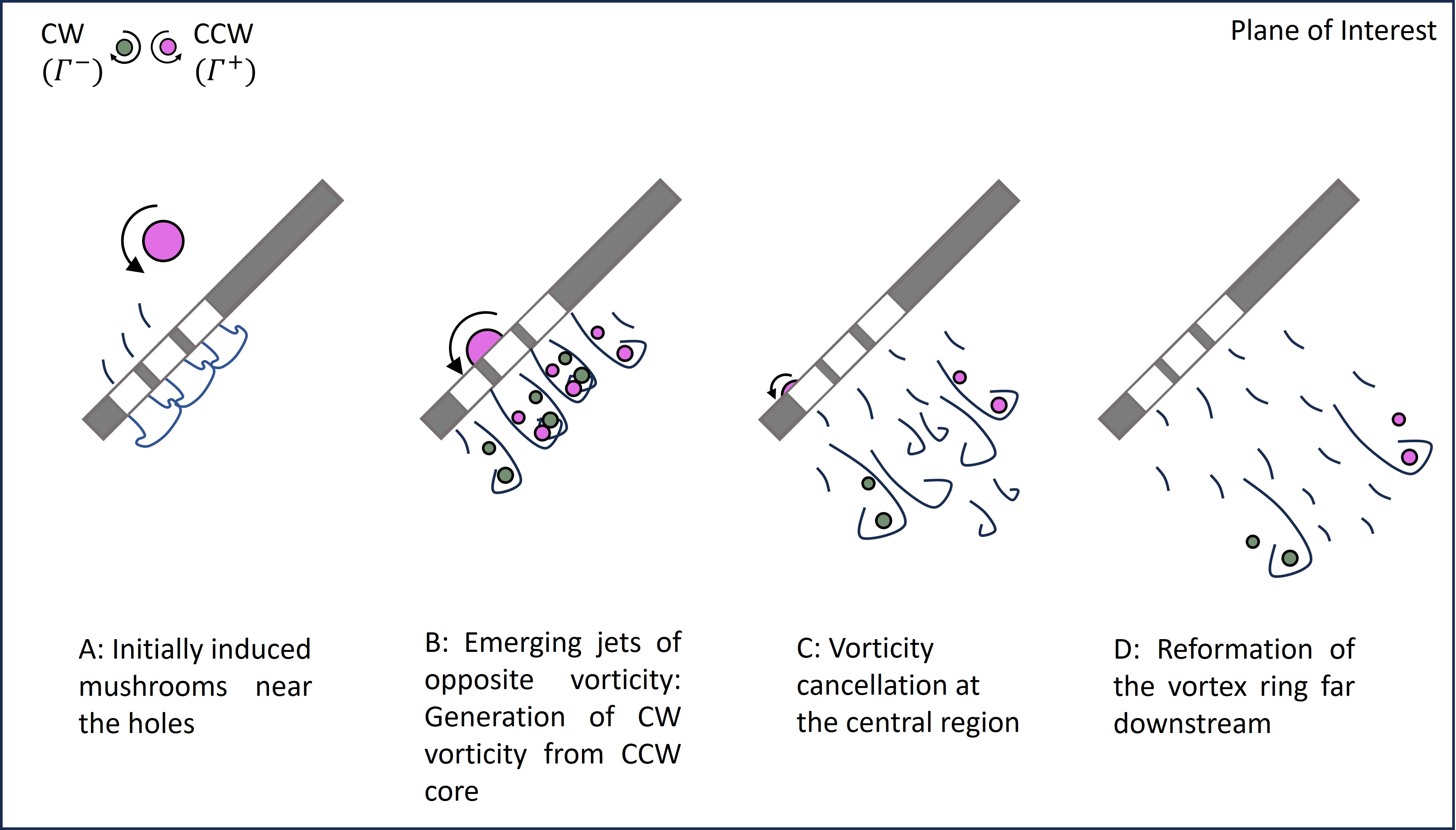
Figure 17: A general schematic diagram depicting the chain of events and the generation of reformed vortex by the interaction of single half of the vortex ring. The figure is not to scale is meant for qualitative description.

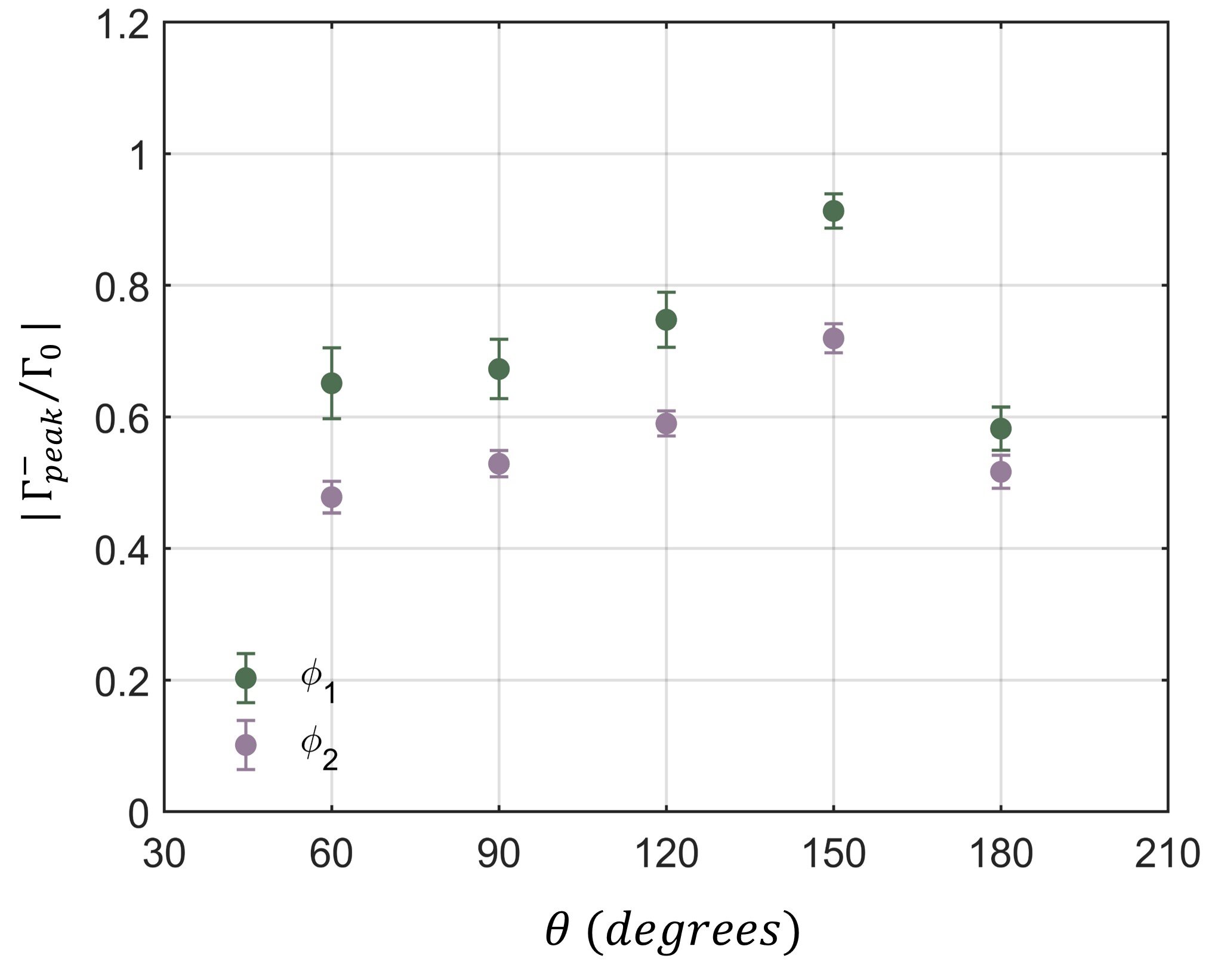
Figure 18: Variation of the non-dimensional negative circulation peak in the downstream region with $\theta$.

We see that a single half of vortex ring on interaction with a single half of the perforated surface results in the formation of a full vortex ring (figure 6). A schematic to understand this phenomenon has been provided in figure 17. As we consider the right hand side of the interaction zone, the CCW part of the vortex ring interacts with the perforated surface to generate vorticity of both CW and CCW to ultimately reform a vortex ring. Although, the values of positive circulation (CCW) remains higher (check figure 15), the value of negative circulation is strongly dependent on the $\theta$ value. Figure 18 is plotted to show the variation of negative circulation peak for both the values of $\phi$ at different values of $\theta$. It can be seen that for $\phi_{2}$, the strength of the negative circulation generated is consistently lesser for all values of $\theta$ compared to that in $\phi_{1}$. With increase in the value of $\theta$, the normalized negative circulation increases that reaches a peak at $\theta$ = 150° before falling significantly at $\theta$ = 180° (considered a half part). The fall is expected since for $\theta$ = 180° we see a very symmetric nature of the circulation produced when the whole downstream flow field is considered (figure S6). The negative circulation region shifts towards the central region which is not fully considered here. Further analysis of the reformed vortex ring can provide deeper insights into the symmetricity and contribution of the negative circulation on its overall strength.

To summarize the vorticity dynamics, we observe a more distributed flow field in case of ${\phi_{2}}$ compared to cases with ${\phi_{1}}$. The jet like features coming out of ${\phi_{1}}$ and their interaction results in the shedding of multiple small vortical features. The vorticity cancellation seems to be less intense in case of ${\phi_{2}}$ because of the generation of dominant vorticity patches at the outer edges of the flow and smaller patches at the central region. However, it is difficult to precisely quantify the vorticity cancellation phenomenon owing to the 3-dimensional nature of the flow downstream. For all the cases except for $\theta$=150° where the fluids from the two halves of the surface interacts with each other, we observe the formation of two primary vortical structures that propel in the direction roughly normal to the surface (except for ${\phi_{2}\theta^{60}}$). The interaction between the flows between the two halves results in the creation or imbalance of vorticity from the flow shearing between different rotating structures. What we also infer is that by keeping a perforated surface with 60°$\leq$$\theta$$<$150° of the kind used in the present work ($d_{h}$ = h), a vortex ring is split in to two vortex rings that propels in the direction imposed by the plate inclination. The process involves the generation of jets of opposite vorticity that results in the reformed vortex. Such arrangements can be used to manipulate flow at various scales. Further, a value near to $\theta$=150° can be utilized to suppress the re-formation of the vortex ring after interacting with perforated plates.

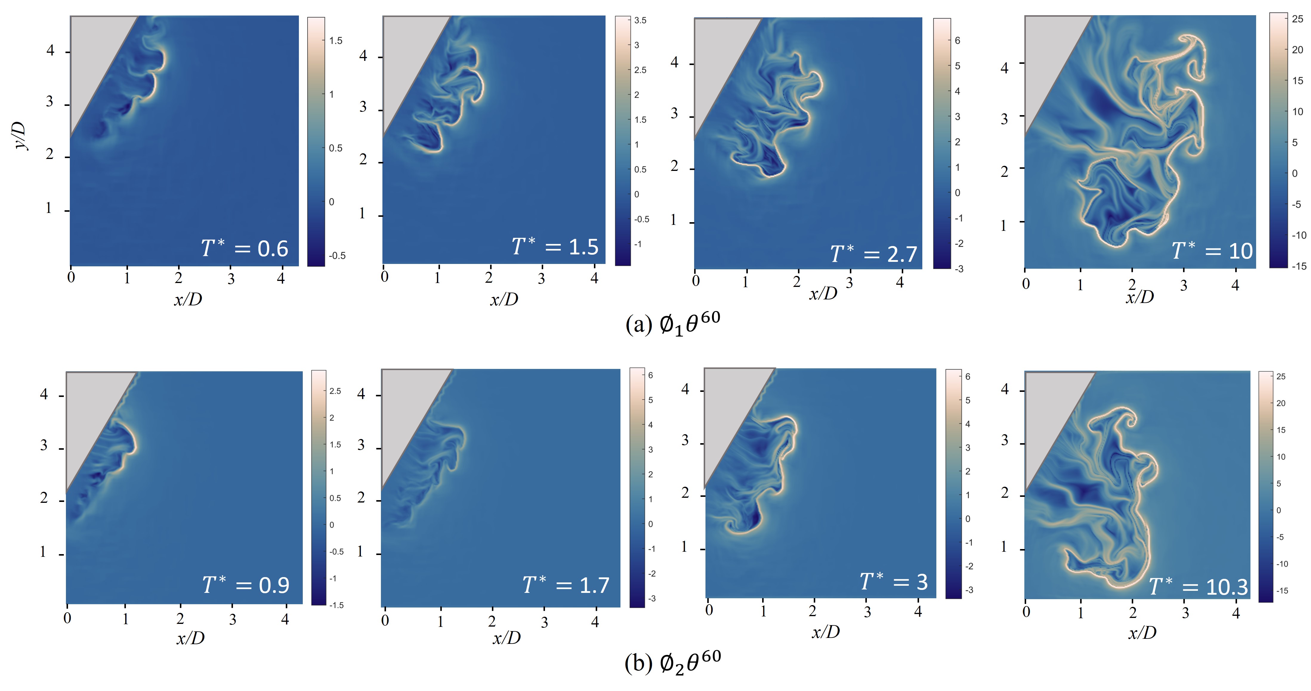
Figure 19: Backward FTLE field for (a) ${\phi_{1}\theta^{60}}$ and (b) ${\phi_{2}\theta^{60}}$ shown at different $T^{*}$ corresponding to figure 10.

3.3.3 Lagrangian analysis

Figure 19, 20, 21 and S7 shows the backward FTLE fields for $\theta$ = 60° , 120°  150° and 180° respectively. FTLE fields are shown at the same $T^{*}$ for which the vorticity contours are plotted (in figures 10, 12, 13 and 14). Our primary aim is to elucidate if the jets emerging out of the permeable surface mix at all and if it does, how and when. Although, a lot has been discussed in details about the interaction of jets in the above sections, we finally want to conclude our analysis with a qualitative evaluation of the FTLE fields digging deeper into the dynamics of out coming jets from the holes. The LCS are the ridges of the FTLE fields that is transverse to the direction of minimum curvature (Haller, 2001). Based on the system’s dynamical behavior, the LCS in the flow fields represent surfaces that does not allow transport across it. We plot the FTLE values by integrating backward in time that yields attractive FTLE ridges. Since, we use different integration time for each of the $T^{*}$, the FTLE range obtained for each of the frame varies. However, bringing out the bright ridges to understand the mixing dynamics remains the central theme of this exercise.

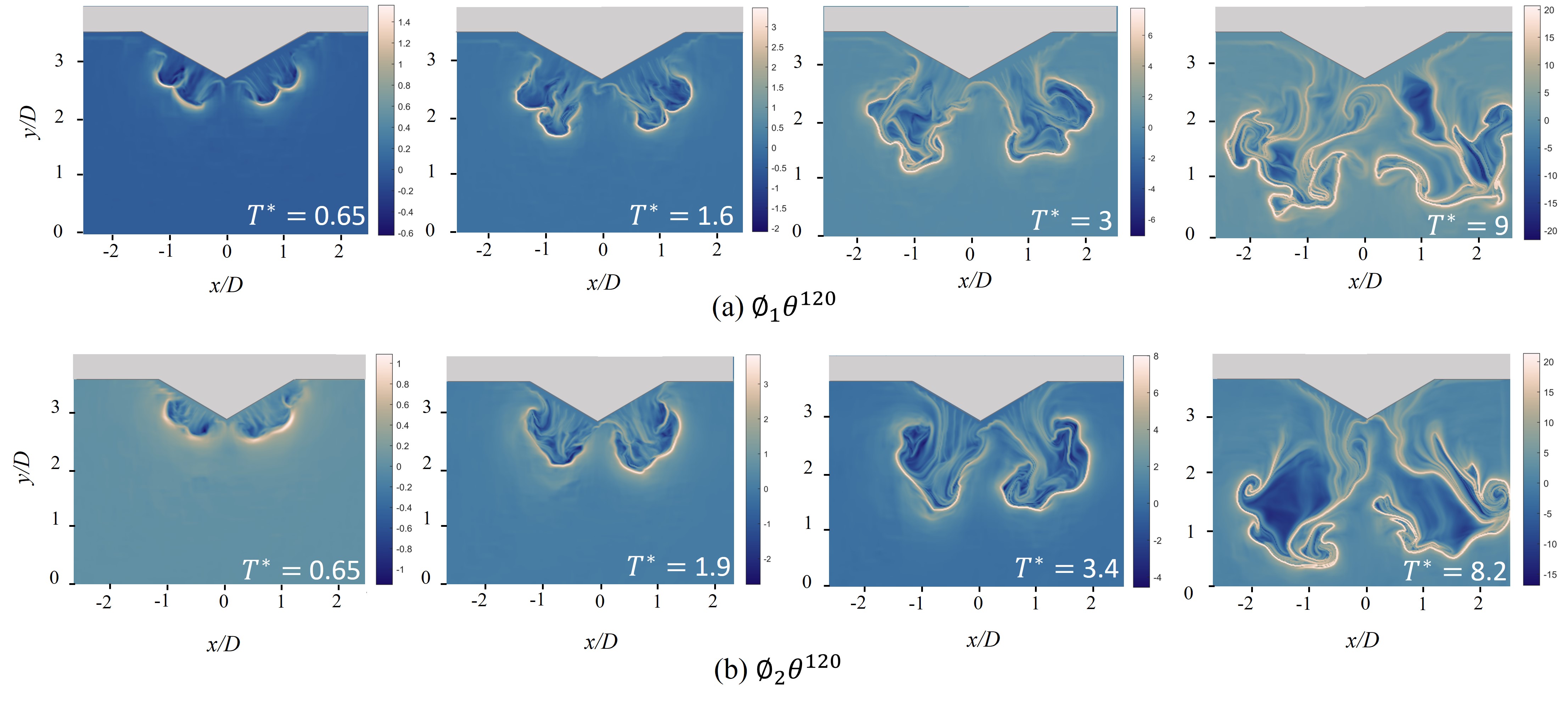
Figure 20: Backward FTLE field for (a) ${\phi_{1}\theta^{120}}$ and (b) ${\phi_{2}\theta^{120}}$ shown at different $T^{*}$ corresponding to figure 12.

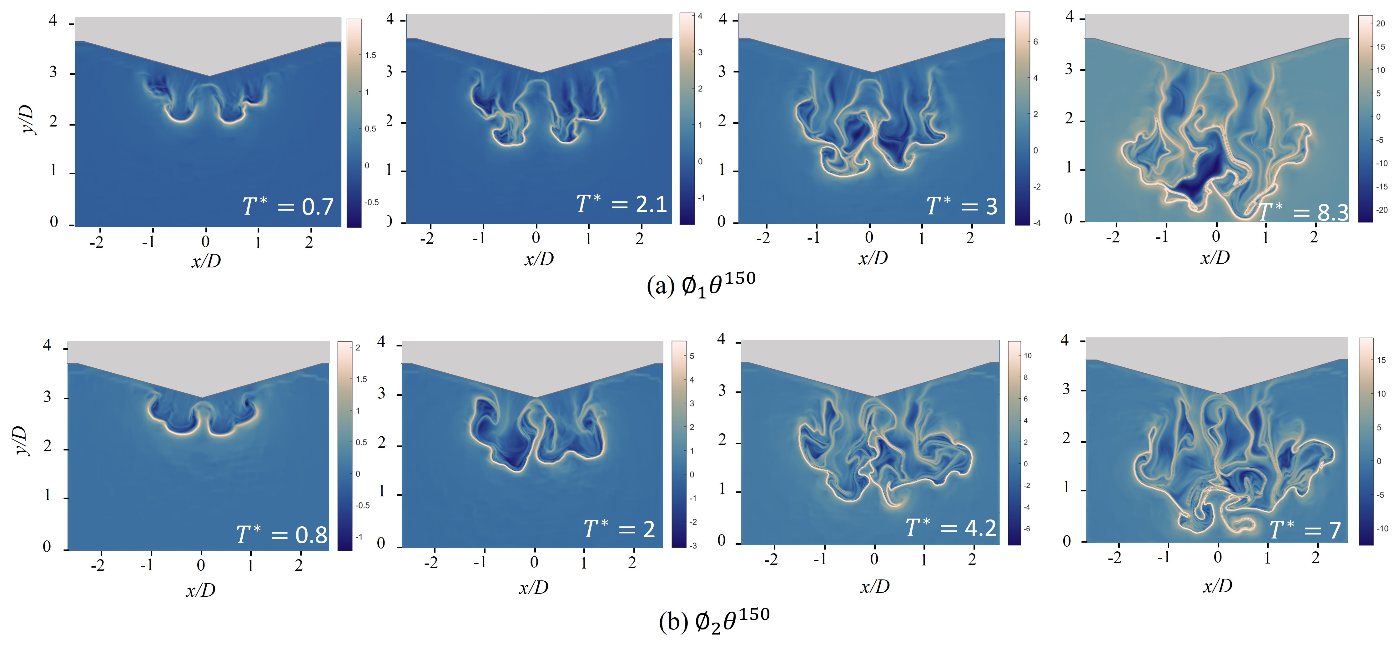
Figure 21: Backward FTLE field for (a) ${\phi_{1}\theta^{150}}$ and (b) ${\phi_{2}\theta^{150}}$ shown at different $T^{*}$ corresponding to figure 13.

From the first instance, brighter ridges between the jets coming out of the perforated surface can be detected in case of ${\phi_{1}\theta^{60}}$ unlike that for ${\phi_{2}\theta^{60}}$ (figure 19) where a continuous front of the attractive LCS develops. The ridge front of the flow structure is brightest at the farthest side of the apex due to the early emergence of flow for ${\theta}$ = 60° as discussed earlier. For ${\phi_{1}\theta^{60}}$, the separation between the jets can be clearly observed at $T^{*}$ = 1.5 that further starts to blur out with the passage of time. However, for ${\phi_{2}\theta^{60}}$ we see very less amount of bright separatrices appearing between the jets indicating towards the mixing of flow at very early stages of emerging out. The flow structures at the later stages corresponds well with the vorticity contours in figure 10. Similar patterns can be observed for ${\theta}$ = 120°(figure 20) with highly mixed flows for ${\phi_{2}\theta^{120}}$. We see no interaction between the ridges of the other halves of the surface and neat vortical structures develop. In case of ${\phi_{1}\theta^{150}}$ (figure 21), the interaction of the flow from the other halves can be seen around $T^{*}$ = 3 whereas this begins much early for ${\phi_{2}\theta^{150}}$. At further instances, very chaotic flow with random distribution of attractive ridges develops which was educed from PLIF and PIV results. Finally, with the attractive LCS we could successfully explain the various events taking place during the interaction process. Although we do not show the forward FTLE or the repelling ridges, it can effectively be utilized to understand the entrainment quality associated with the flow structures that reform in the downstream region after interacting with the perforated surface. Furthermore, a rigorous quantitative analysis of the ridges can bring out more insights into the mixing phenomenon among the jets.

4 Summary and Conclusions

Experiments were conducted to explore the interaction dynamics of a vortex ring ($Re_{\Gamma}$ = 11500) impinging on perforated surface (${\phi_{1}}$ = 0.24 and ${\phi_{2}}$ = 0.44) with different included angles (${\theta}$ = 60°- 180°) using PLIF, PIV, Lagrangian FTLE and $\Gamma_{2}$ vortex identification techniques. By changing the the value of $\theta$ the interaction process is altered significantly. The early interaction of the vortex ring with the perforated surface results in a sequential ejection of the fluid and a reduction in number of ejecting holes with increase in the ${\theta}$ value, a phenomenon very well captured by the PLIF images. Due to higher proximity of the holes in case of ${\phi_{2}}$, the jets are seen to interact immediately as it start to emerge out of the perforated surface. Whereas for ${\phi_{1}}$, the jets interact much later and their development is characterized by the occurrence of K-H instability at its edges.

An interesting phenomenon involving the development of mushroom shaped features is reported. The fluid ahead of the vortex ring moving with the induced velocity crosses the perforated surface earlier than the main vortex resulting in the growth of dormant mushroom structures which is later caught by the faster main flow. These structures are a result of placing a perforated plate in the path of a vortex ring and imparts initial instability to the jet structures.

From the time series contour plot of $V_{mag}^{*}$, we show that the sequential ejection of the vortex ring in the forms of jets. Further, a change in the slope in the $V_{mag}^{*}$ peak for $\theta$ $>$ 90° with time indicate towards the shift of the first ejection hole of the vortex ring. This marks a transition point from where the flow starts to tend towards ${\theta}$ = 180°. The vorticity dynamics of the flow for all the cases has been discussed in details supported by the vortex centres that are identified using the $\Gamma_{2}$ method. The formation, interaction and cancellation of the vortical structures both in the form of jets and circular patches are shown. The movement of the cores and their interaction at $\theta$ = 150° is shown along with the generation of multiple small scale vortical zones. The vorticity cancellation phenomenon occurs for both the ${\phi}$ values but differently, which ultimately results in the preservation of the velocity profile of the vortex ring leading to the reformation of vortex ring at far downstream except in $\theta$ = 150°. Further analysis of the development of circulation over time revealed the occurrence of an imbalance in the vorticity due to the shearing of the flows from two halves of the surface in case of $\theta$ = 150°. The peak of both the positive and negative circulation achieves similar non-dimensional circulation but diverges after a point of time and behaves like $\theta$ = 180°case suggesting the fading effect of the effect of $\theta$. The Lagrangian FTLE fields finally confirmed towards the sequential emerging, early interaction of flow from holes in case of $\phi_{2}$ and and interaction of flow from other halves resulting in turbulent structure with random attractive LCS.

Inline with the objectives identified in section 1, we have successfully answered how the vortex ring emerges out of inclined porous surfaces and the effect of different $\theta$ on the downstream flow. The behaviour and interaction of jet was also studied however, a more rigorous analysis of the emerging jets can reveal more insights into the phenomenon. Finally, the effect of $\phi$ was seen to be significant in changing the flow dynamics.

It is worth mentioning that by placing a perforated plate with different $\theta$ values, a reformed vortex can be generated from each side i.e., a single vortex ring is capable of generating two reformed vortex rings. Further, this generation of reformed vortex ring can also be suppressed by maintaining the $\theta$ value near to 150° between the surfaces. Such results can prove to be useful for flow control and manipulation purposes.

5 Acknowledgement

S. Jain and S.R Rao would like to thank the Prime Minister Research Fellowship (PMRF) for the financial support.

6 Supplementary Data

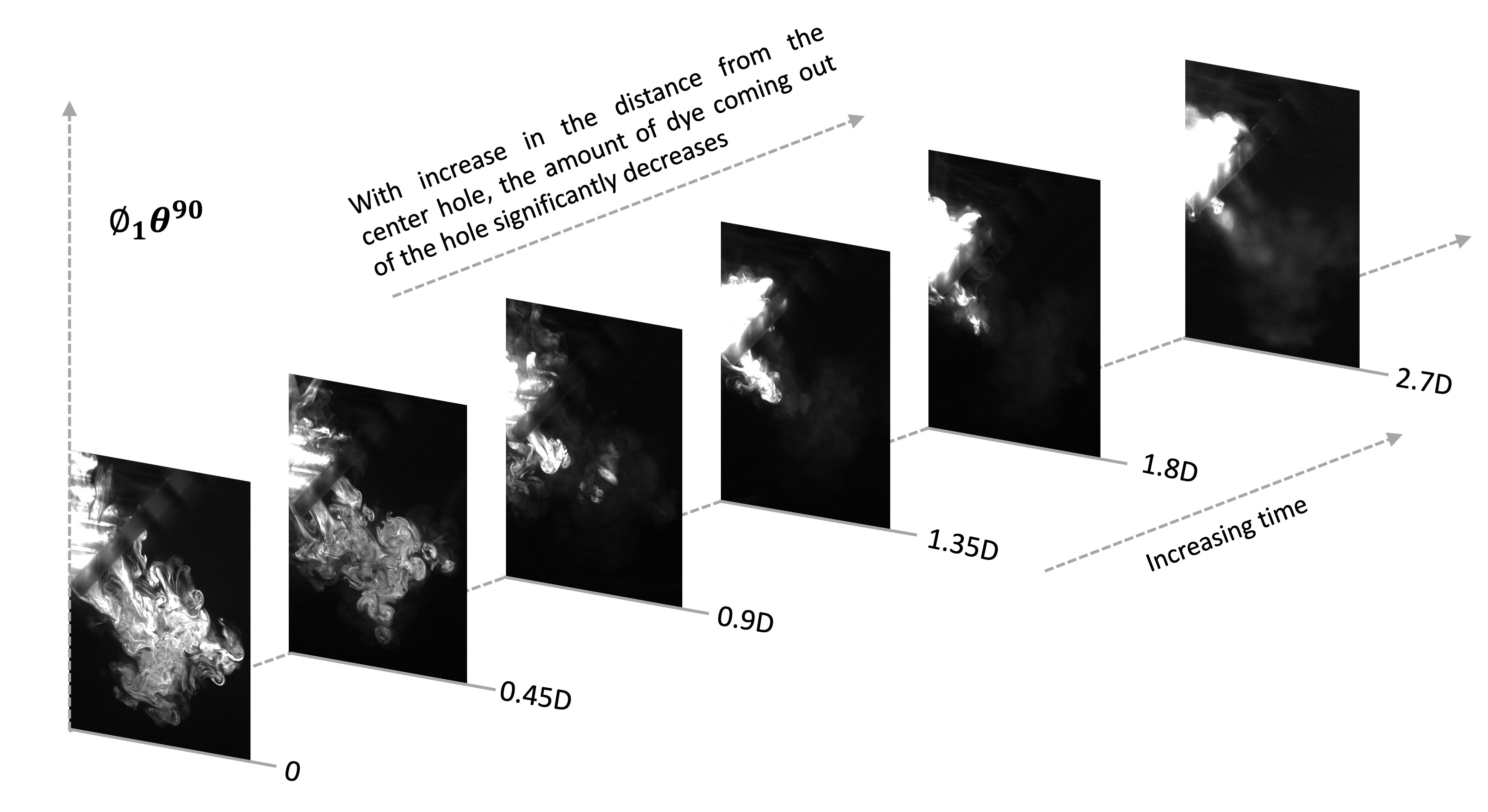
Figure 22: Figure S1: PLIF images after interaction of vortex ring with perforated surface for ${\phi_{2}\theta^{150}}$ captured at different planes measured from the hole aligned with the vortex ring’s translational axis. For 1.35D and beyond, the images are captured at later times since the fluid comes out of the farther holes much later after the interaction at 0D takes place.

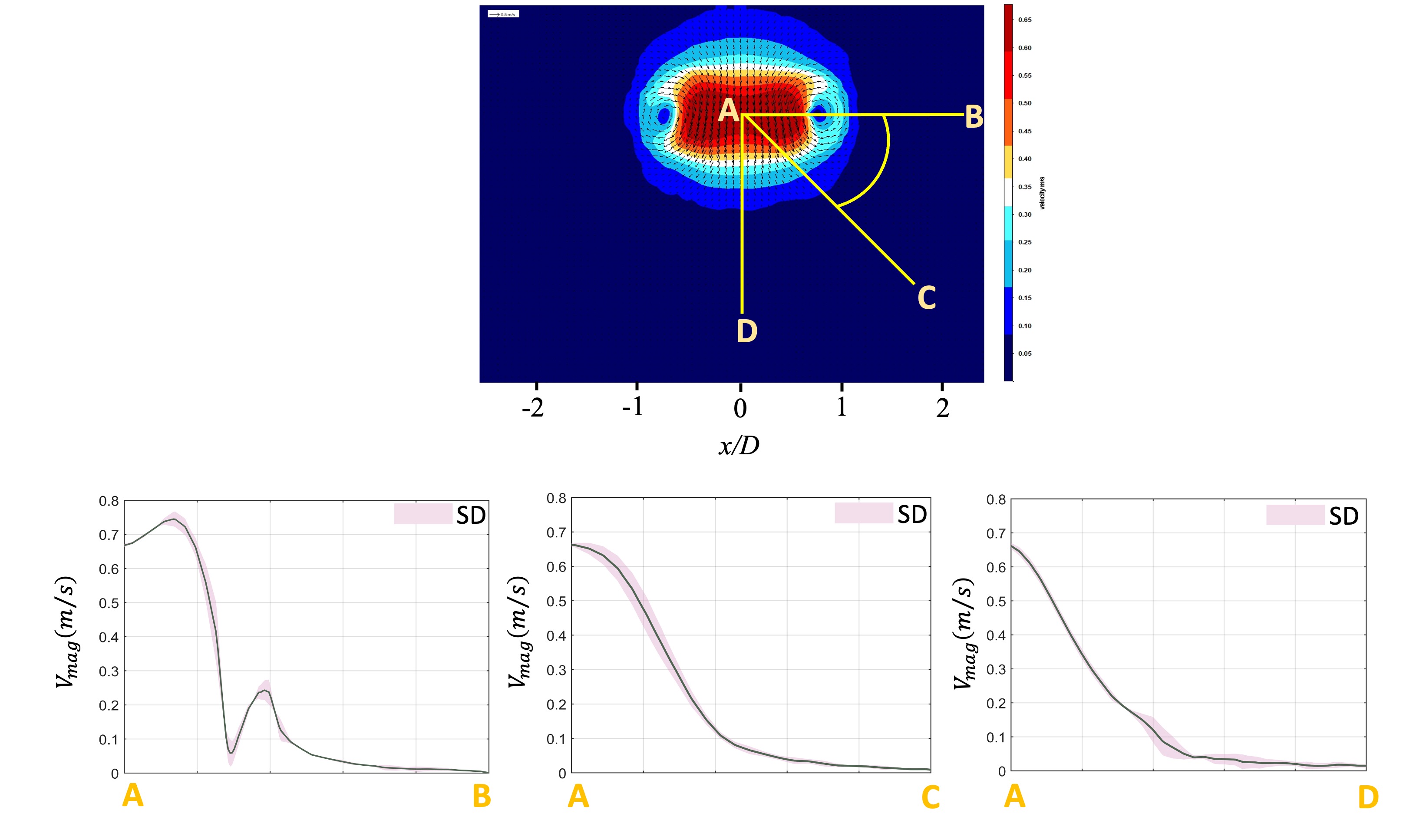
Figure 23: Figure S2: The velocity magnitude $V_{m}ag$ along the lines AB, AC and AD where A corresponds to the center of the vortex ring. The angle between AB-AC and AC-AD is 45°. The shaded region represents the standard deviation (SD).

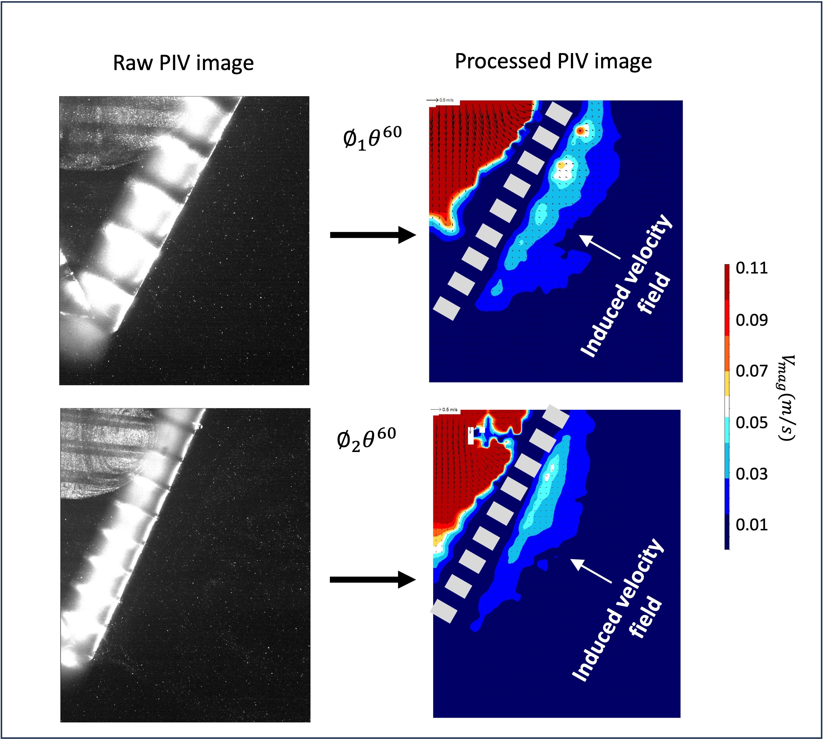
Figure 24: Figure S3: The induced velocity field across the perforated surface for $\theta$=60°is shown. The left column represents the raw PIV images, and the corresponding processed image is shown in the right column.

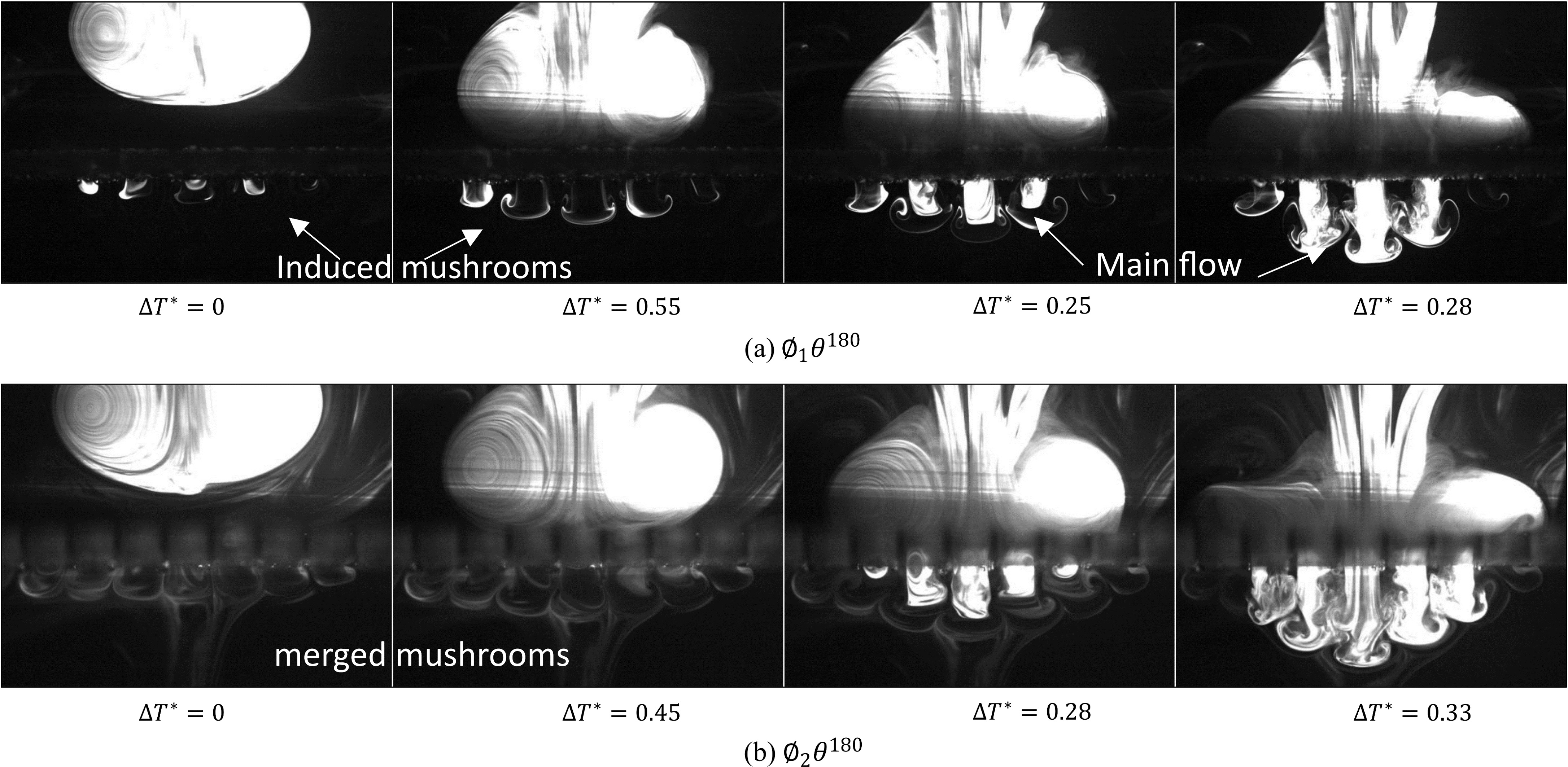
Figure 25: Figure S4: The PLIF images for ${\phi_{1}\theta^{180}}$ and ${\phi_{2}\theta^{180}}$ depicting the initial jet instability due to mushroom formation. Here, $\Delta^{*}$= is the difference in $T^{*}$. The scale represents 5 mm.

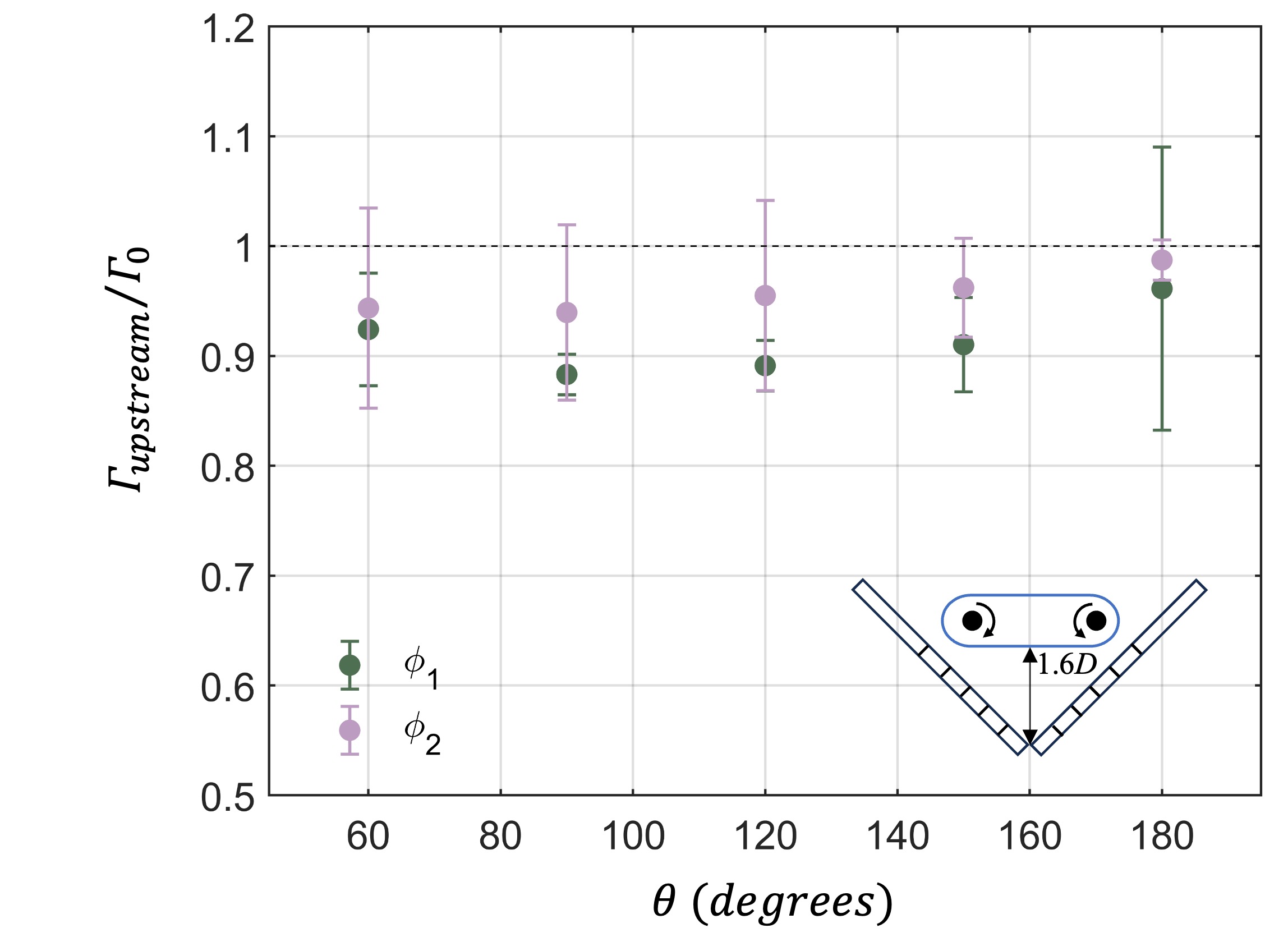
Figure 26: Figure S5: The circulation of the vortex ring just before the interaction as shown in the inset normalized with the circulation of free vortex $(\Gamma_{0})$. The error bars represent the standard deviation (SD). For all the case, a minimal change in the circulation value is observed with respect to $(\Gamma_{0})$ with a maximum reduction of around   10%. The values are particularly lower for the case of $\phi_{1}$ at all the $\theta$ which has a lower open area and behaves more like impermeable wall compared to $\phi_{2}$. It is expected that larger open area cases will behave more like free vortex case (i.e., without any surface) and the values should be nearer to 1. As the $\theta$ value reaches 180 °, the ratio approaches the value 1 for both the case. The presence of the wall near the vortex ring before the interaction as shown in the inset contaminates the PIV data and hence, we see higher values of SD values.

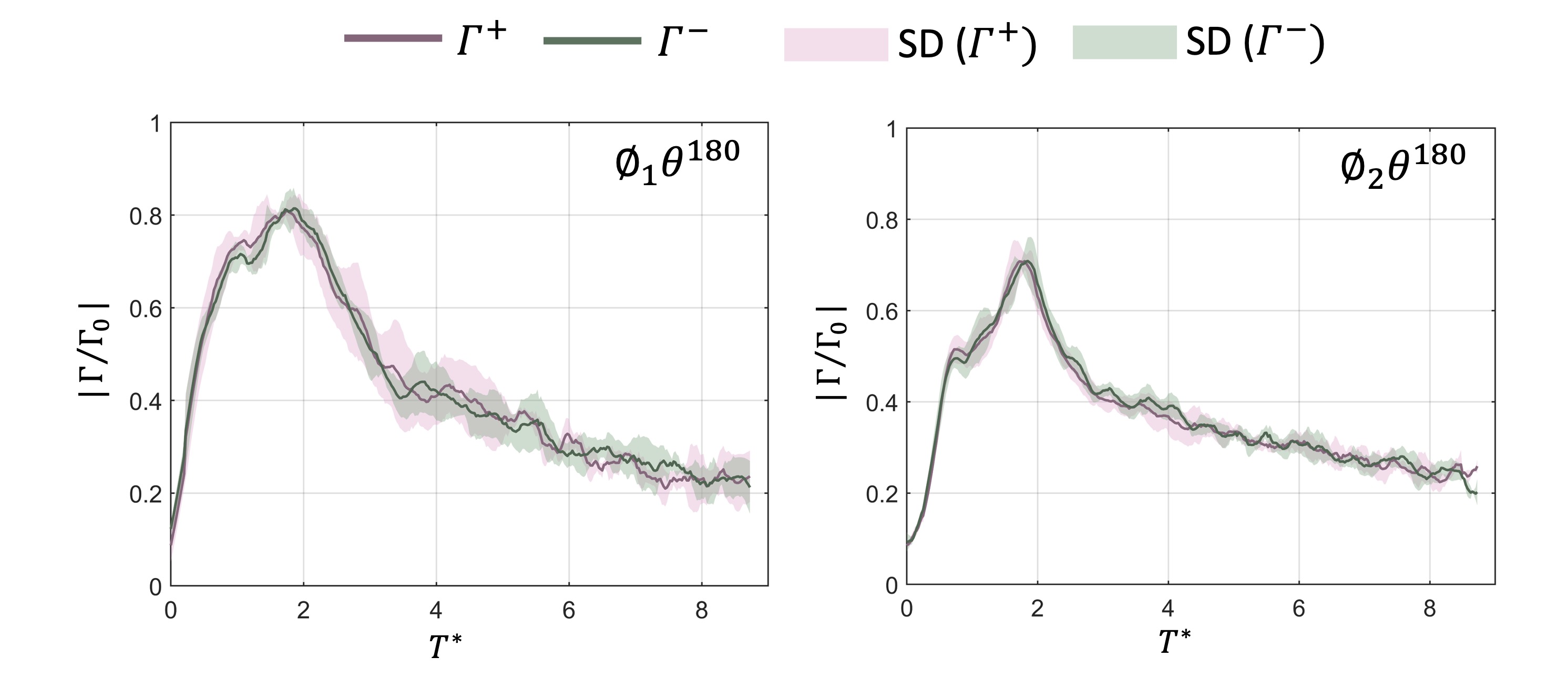
Figure 27: Figure S6: The variation of absolute values of non-dimensional positive and negative circulation in the downstream region of the flow field after interaction for $\theta$ = 180°cases with $T^{*}$. Here, $T^{*}$ = 0 represents the instance at which the velocity vectors become detectable after interaction in the downstream region. SD represents the standard deviation of the data.

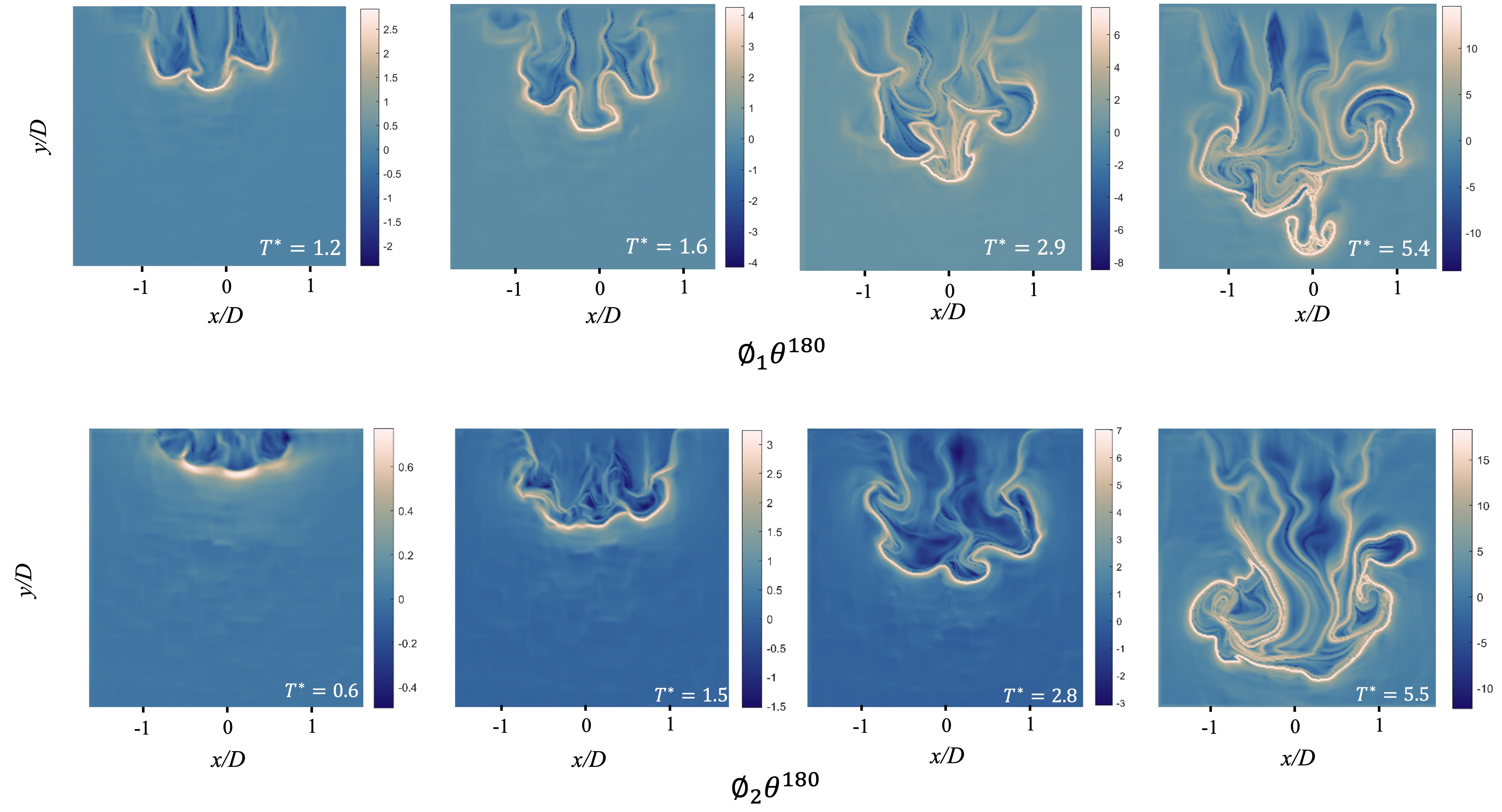
Figure 28: Figure S7: Backward FTLE field for (a) ${\phi_{1}\theta^{180}}$ and (b) ${\phi_{2}\theta^{180}}$ shown at different $T^{*}$ corresponding to figure 14 (in the main manuscript).

References

- Adhikari & Lim (2009) Adhikari, D & Lim, T T 2009 The impact of a vortex ring on a porous screen. Fluid Dynamics Research 41 (5), 051404.
- Ahmed & Erath (2023) Ahmed, Tanvir & Erath, Byron D. 2023 Experimental study of vortex ring impingement on concave hemispherical cavities. Journal of Fluid Mechanics 967, A38, a38.
- ALLEN et al. (2007) ALLEN, J. J., JOUANNE, Y. & SHASHIKANTH, B. N. 2007 Vortex interaction with a moving sphere. Journal of Fluid Mechanics 587, 337–346.
- Amitay et al. (2001) Amitay, Michael, Smith, Douglas R., Kibens, Valdis, Parekh, David E. & Glezer, Ari 2001 Aerodynamic flow control over an unconventional airfoil using synthetic jet actuators. AIAA Journal 39 (3), 361–370, arXiv: https://doi.org/10.2514/2.1323.
- An et al. (2016) An, Duo, Warning, Alex, Yancey, Kenneth G., Chang, Chun-Ti, Kern, Vanessa R., Datta, Ashim K., Steen, Paul H., Luo, Dan & Ma, Minglin 2016 Mass production of shaped particles through vortex ring freezing. Nature Communications 7 (1), 12401.
- Biswas & Govardhan (2023) Biswas, Subhajit & Govardhan, Raghuraman N. 2023 Vortex ring and bubble interaction: Effects of bubble size on vorticity dynamics and bubble dynamics. Physics of Fluids 35 (8), 083328.
- Cheng et al. (2014) Cheng, M., Lou, J. & Lim, T. T. 2014 A numerical study of a vortex ring impacting a permeable wall. Physics of Fluids 26 (10), 103602, arXiv: https://doi.org/10.1063/1.4897519.
- Cheng et al. (2018) Cheng, M., Lou, J. & Lim, T. T. 2018 Numerical simulation of head-on collision of two coaxial vortex rings. Fluid Dynamics Research 50 (6), 065513.
- Chu et al. (1993) Chu, Chin‐Chou, Wang, Chi‐Tzung & Hsieh, Chang‐Shyue 1993 An experimental investigation of vortex motions near surfaces. Physics of Fluids A: Fluid Dynamics 5 (3), 662–676, arXiv: https://doi.org/10.1063/1.858650.
- Couch & Krueger (2011) Couch, Lauren D. & Krueger, Paul S. 2011 Experimental investigation of vortex rings impinging on inclined surfaces. Experiments in Fluids 51 (4), 1123–1138.
- Dabiri et al. (2005) Dabiri, John O., Colin, Sean P., Costello, John H. & Gharib, Morteza 2005 Flow patterns generated by oblate medusan jellyfish: field measurements and laboratory analyses. Journal of Experimental Biology 208 (7), 1257–1265.
- Didden (1979) Didden, Norbert 1979 On the formation of vortex rings: Rolling-up and production of circulation. Zeitschrift für angewandte Mathematik und Physik ZAMP 30 (1), 101–116.
- Espa et al. (2012) Espa, S., Badas, M.G., Fortini, S., Querzoli, G. & Cenedese, A. 2012 A lagrangian investigation of the flow inside the left ventricle. European Journal of Mechanics - B/Fluids 35, 9–19, cardiovascular Flows.
- Gan et al. (2012) Gan, L., Dawson, J. R. & Nickels, T. B. 2012 On the drag of turbulent vortex rings. Journal of Fluid Mechanics 709, 85–105.
- Gharib et al. (1998) Gharib, M., Rambod, E. & Shariff, K. 1998 A universal time scale for vortex ring formation. Journal of Fluid Mechanics 360, 121–140.
- Glezer (1988) Glezer, Ari 1988 The formation of vortex rings. The Physics of Fluids 31 (12), 3532–3542.
- Glezer & Coles (1990) Glezer, Ari & Coles, Donald 1990 An experimental study of a turbulent vortex ring. Journal of Fluid Mechanics 211, 243–283.
- Graftieaux et al. (2001) Graftieaux, Laurent, Michard, Marc & Grosjean, Nathalie 2001 Combining piv, pod and vortex identification algorithms for the study of unsteady turbulent swirling flows. Measurement Science and Technology 12 (9), 1422.
- Hadziabdic & Hanjalic (2008) Hadziabdic, M. & Hanjalic, K. 2008 Vortical structures and heat transfer in a round impinging jet. Journal of Fluid Mechanics 596, 221–260.
- Haller (2000) Haller, G. 2000 Finding finite-time invariant manifolds in two-dimensional velocity fields. Chaos: An Interdisciplinary Journal of Nonlinear Science 10 (1), 99–108, arXiv: https://pubs.aip.org/aip/cha/article-pdf/10/1/99/7861759/99_1_online.pdf.
- Haller (2001) Haller, G. 2001 Distinguished material surfaces and coherent structures in three-dimensional fluid flows. Physica D: Nonlinear Phenomena 149 (4), 248–277.
- Haller (2015) Haller, George 2015 Lagrangian coherent structures. Annual Review of Fluid Mechanics 47 (1), 137–162, arXiv: https://doi.org/10.1146/annurev-fluid-010313-141322.
- Haller & Sapsis (2011) Haller, George & Sapsis, Themistoklis 2011 Lagrangian coherent structures and the smallest finite-time Lyapunov exponent. Chaos: An Interdisciplinary Journal of Nonlinear Science 21 (2), 023115, arXiv: https://pubs.aip.org/aip/cha/article-pdf/doi/10.1063/1.3579597/14602779/023115_1_online.pdf.
- Hrynuk et al. (2018) Hrynuk, John T., Stutz, Colin M. & Bohl, Doug G. 2018 Experimental Measurement of Vortex Ring Screen Interaction Using Flow Visualization and Molecular Tagging Velocimetry. Journal of Fluids Engineering 140 (11), 111401, arXiv: https://asmedigitalcollection.asme.org/fluidsengineering/article-pdf/140/11/111401/6060391/fe_140_11_111401.pdf.
- Hrynuk et al. (2012) Hrynuk, John T., Van Luipen, Jason & Bohl, Douglas 2012 Flow visualization of a vortex ring interaction with porous surfaces. Physics of Fluids 24 (3), 037103, arXiv: https://doi.org/10.1063/1.3695377.
- Hu & Peterson (2018) Hu, JiaCheng & Peterson, Sean D. 2018 Vortex ring impingement on a wall with a coaxial aperture. Phys. Rev. Fluids 3, 084701.
- Hussain & Jeong (1995) Hussain, Fazle & Jeong, Jinhee 1995 On the identification of a vortex. Journal of Fluid Mechanics 285, 69–94.
- Jain et al. (2023) Jain, Siddhant, Sharma, Shubham, Roy, Durbar & Basu, Saptarshi 2023 Vortical cleaning of oil-impregnated porous surfaces. Phys. Rev. Fluids 8, 044701.
- Jha & Govardhan (2015) Jha, Narsing K. & Govardhan, R. N. 2015 Interaction of a vortex ring with a single bubble: bubble and vorticity dynamics. Journal of Fluid Mechanics 773, 460–497.
- Kasten et al. (2010) Kasten, Jens, Petz, Christoph, Hotz, Ingrid, Hege, Hans-Christian, Noack, Bernd R. & Tadmor, Gilead 2010 Lagrangian feature extraction of the cylinder wake. Physics of Fluids 22 (9), 091108, arXiv: https://pubs.aip.org/aip/pof/article-pdf/doi/10.1063/1.3483220/15754576/091108_1_online.pdf.
- Krieg & Mohseni (2013) Krieg, Michael & Mohseni, Kamran 2013 On approximating the translational velocity of vortex rings. Journal of Fluids Engineering 135 (12), 124501.
- Lim (1989) Lim, T. T. 1989 An experimental study of a vortex ring interacting with an inclined wall. Experiments in Fluids 7 (7), 453–463.
- Lim & Nickels (1992) Lim, T. T. & Nickels, T. B. 1992 Instability and reconnection in the head-on collision of two vortex rings. Nature 357 (6375), 225–227.
- Lim & Nickels (1995) Lim, T. T. & Nickels, T. B. 1995 Vortex Rings (in Fluid Vortices). Dordrecht: Springer Netherlands.
- Liu & Sullivan (1996) Liu, Tianshu & Sullivan, J.P. 1996 Heat transfer and flow structures in an excited circular impinging jet. International Journal of Heat and Mass Transfer 39 (17), 3695–3706.
- Lundgren et al. (1992) Lundgren, T. S., Yao, J. & Mansour, N. N. 1992 Microburst modelling and scaling. Journal of Fluid Mechanics 239, 461–488.
- Mathur et al. (2007) Mathur, Manikandan, Haller, George, Peacock, Thomas, Ruppert-Felsot, Jori E. & Swinney, Harry L. 2007 Uncovering the lagrangian skeleton of turbulence. Phys. Rev. Lett. 98, 144502.
- Maxworthy (1972) Maxworthy, T. 1972 The structure and stability of vortex rings. Journal of Fluid Mechanics 51 (1), 15–32.
- Maxworthy (1977) Maxworthy, T. 1977 Some experimental studies of vortex rings. Journal of Fluid Mechanics 81 (3), 465–495.
- Mohseni & Gharib (1998) Mohseni, Kamran & Gharib, Morteza 1998 A model for universal time scale of vortex ring formation. Physics of Fluids 10 (10), 2436–2438.
- Morris & Williamson (2020) Morris, Sarah E. & Williamson, C. H. K. 2020 Impingement of a counter-rotating vortex pair on a wavy wall. Journal of Fluid Mechanics 895, A25.
- Naaktgeboren et al. (2012) Naaktgeboren, Christian, Krueger, Paul S. & Lage, José L. 2012 Interaction of a laminar vortex ring with a thin permeable screen. Journal of Fluid Mechanics 707, 260–286.
- Naitoh et al. (1995) Naitoh, Takashi, Sun, Baoguo & Yamada, Hideo 1995 A vortex ring travelling across a thin circular cylinder. Fluid Dynamics Research 15 (1), 43–56.
- New et al. (2020) New, T. H., Long, J., Zang, B. & Shi, Shengxian 2020 Collision of vortex rings upon v-walls. Journal of Fluid Mechanics 899, A2, a2.
- New et al. (2016) New, T. H., Shi, Shengxian & Zang, B. 2016 Some observations on vortex-ring collisions upon inclined surfaces. Experiments in Fluids 57 (6), 109.
- New & Zang (2017) New, T. H. & Zang, B. 2017 Head-on collisions of vortex rings upon round cylinders. Journal of Fluid Mechanics 833, 648–676.
- Olascoaga et al. (2013) Olascoaga, M. J., Beron-Vera, F. J., Haller, G., Triñanes, J., Iskandarani, M., Coelho, E. F., Haus, B. K., Huntley, H. S., Jacobs, G., Kirwan Jr., A. D., Lipphardt Jr., B. L., Özgökmen, T. M., H. M. Reniers, A. J. & Valle-Levinson, A. 2013 Drifter motion in the gulf of mexico constrained by altimetric lagrangian coherent structures. Geophysical Research Letters 40 (23), 6171–6175, arXiv: https://agupubs.onlinelibrary.wiley.com/doi/pdf/10.1002/2013GL058624.
- Olascoaga & Haller (2012) Olascoaga, Maria J. & Haller, George 2012 Forecasting sudden changes in environmental pollution patterns. Proceedings of the National Academy of Sciences 109 (13), 4738–4743.
- Orlandi (1990) Orlandi, Paolo 1990 Vortex dipole rebound from a wall. Physics of Fluids A: Fluid Dynamics 2 (8), 1429–1436.
- Per M. et al. (2016) Per M., Arvidsson, Sandor, J. Kovács, Johannes, Töger, Rasmus, Borgquist, Heiberg, Einar, Carlsson, Marcus & Arheden, Håkan 2016 Vortex ring behavior provides the epigenetic blueprint for the human heart. Scientific Reports 6 (1), 22021, arXiv: https://doi.org/10.1038/srep22021.
- Saffman (1970) Saffman, P. G. 1970 The velocity of viscous vortex rings. Studies in Applied Mathematics 49 (4), 371–380.
- Shadden et al. (2007) Shadden, S. C., KATIJA, K., ROSENFELD, M., MARSDEN, J. E. & DABIRI, J. O. 2007 Transport and stirring induced by vortex formation. Journal of Fluid Mechanics 593, 315–331.
- Shadden et al. (2005) Shadden, Shawn C., Lekien, Francois & Marsden, Jerrold E. 2005 Definition and properties of lagrangian coherent structures from finite-time lyapunov exponents in two-dimensional aperiodic¬†flows. Physica D: Nonlinear Phenomena 212 (3), 271–304.
- Sharma et al. (2022) Sharma, Shubham, Jain, Siddhant, Saha, Abhishek & Basu, Saptarshi 2022 Evaporation dynamics of a surrogate respiratory droplet in a vortical environment. Journal of Colloid and Interface Science 623, 541–551.
- Sharma et al. (2021) Sharma, Shubham, Singh, Awanish Pratap & Basu, Saptarshi 2021 On the dynamics of vortex–droplet co-axial interaction: insights into droplet and vortex dynamics. Journal of Fluid Mechanics 918, A37, a37.
- Shusser & Gharib (2000) Shusser, Michael & Gharib, Morteza 2000 Energy and velocity of a forming vortex ring. Physics of Fluids 12 (3), 618–621.
- Vetel et al. (2009) Vetel, Jerome, Garon, Andre & Pelletier, Dominique 2009 Lagrangian coherent structures in the human carotid artery bifurcation. Experiments in Fluids 46 (6), 1067–1079.
- Walker et al. (1987) Walker, J. D. A., Smith, C. R., Cerra, A. W. & Doligalski, T. L. 1987 The impact of a vortex ring on a wall. Journal of Fluid Mechanics 181, 99–140.
- Wolf et al. (2013) Wolf, M, Ortega-Jimenez, V M & Dudley, R 2013 Structure of the vortex wake in hovering anna’s hummingbirds (calypte anna). Proc Biol Sci 280 (1773), 20132391.
- Xiang et al. (2017) Xiang, Yang, Liu, Hong & Qin, Suyang 2017 A unified energy feature of vortex rings for identifying the pinch-off mechanism. Journal of Fluids Engineering 140 (1), 011203.
- Xu et al. (2019) Xu, Yang, Li, Zhi-Yu, Wang, Jin-Jun & Yang, Li-Jun 2019 On the interaction between turbulent vortex rings of a synthetic jet and porous walls. Physics of Fluids 31 (10), 105112, arXiv: https://doi.org/10.1063/1.5100063.
- Xu et al. (2018) Xu, Yang, Wang, Jin-Jun, Feng, Li-Hao, He, Guo-Sheng & Wang, Zhong-Yi 2018 Laminar vortex rings impinging onto porous walls with a constant porosity. Journal of Fluid Mechanics 837, 729–764.
- You & Moin (2008) You, D. & Moin, P. 2008 Active control of flow separation over an airfoil using synthetic jets. Journal of Fluids and Structures 24 (8), 1349–1357, unsteady Separated Flows and their Control.