Graphical Principal Component Analysis of Multivariate Functional Time Series
Abstract
In this paper, we consider multivariate functional time series with a two-way dependence structure: a serial dependence across time points and a graphical interaction among the multiple functions within each time point. We develop the notion of dynamic weak separability, a more general condition than those assumed in literature, and use it to characterize the two-way structure in multivariate functional time series. Based on the proposed weak separability, we develop a unified framework for functional graphical models and dynamic principal component analysis, and further extend it to optimally reconstruct signals from contaminated functional data using graphical-level information. We investigate asymptotic properties of the resulting estimators and illustrate the effectiveness of our proposed approach through extensive simulations. We apply our method to hourly air pollution data that were collected from a monitoring network in China.
Keywords: Dynamic functional principal component analysis, functional time series, graphical model, weak separability, Whittle likelihood
1 Introduction
Functional data analysis (FDA) techniques have been widely used to study features of randomly sampled curves (Ramsay & Silvermann, 2005; Hsing & Eubank, 2015). As a useful tool for dimension reduction and feature extraction, functional principal component analysis (FPCA) plays a prominent role in the analysis of functional data (James et al., 2000; Yao et al., 2005; Ramsay & Silvermann, 2005). In recent years, with the rapid development of data collection methods, multivariate functional data that possess complex temporal correlation structures have become increasingly available. Examples of such data include age-specific mortality rates (Gao & Shang, 2017; Gao et al., 2019), daily traffic flows (Chiou et al., 2014), and social media post counts (Zhu et al., 2022). To analyze these data, we need to account for both multivariate and temporal correlations. Challenges may arise for FPCA due to the need to simultaneously model such two-way dependencies.
To characterize multivariate dependencies, we utilize the partial correlation graph (Epskamp & Fried, 2018) for a set of random elements, of which some pairs are connected if they are partially correlated. Graphical models provide a powerful framework to describe complex dependencies among random objects, which have been defined for both multivariate variables (Friedman et al., 2001) and multivariate time series (Dahlhaus, 2000; Dahlhaus & Eichler, 2003), and is called the Gaussian graphical model under an additional Gaussian assumption. Recently, Qiao et al. (2019, 2020) extended graphical models to characterize multivariate functional observations. However, these models are only applicable to finite-dimensional functional data. It is not trivial to explore partial correlations among infinite-dimensional functions, as the resulting covariance operator is compact and thus not invertible (Hsing & Eubank, 2015). To solve this problem, Zapata et al. (2022) introduced a separability condition to establish partial correlation graphs for infinite-dimensional curves.
Although the aforementioned works evaluate graphical models of functional data, their benefits for FPCA are rarely discussed. In addition, they may not be appropriate for temporally correlated multivariate functions. Multivariate functions observed over time are called multivariate functional time series (MFTS), which is a generalization of scalar time series to the multivariate functional case. For the FPCA of MFTS, one can employ conventional Karhunen-Loève (KL) expansions (Ramsay & Silvermann, 2005) for each individual functional time series (Gao & Shang, 2017; Gao et al., 2019). However, this method may not be flexible enough to capture serial dependencies within temporally correlated functions. Recently, Hörmann et al. (2015) developed a dynamic functional principal component analysis (DFPCA) approach using a frequency-domain method. With the DFPCA, a univariate functional time series can be optimally reconstructed by using a dynamic KL expansion. In theory, the new representation for functional time series is more general and efficient than the conventional KL expansion. Nonetheless, both of these methods ignore graphical interactions in the MFTS, resulting in a loss of statistical efficiency for FPCAs.
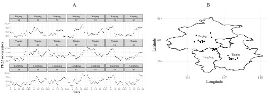
In this article, we consider an MFTS, , where with being the domain of the multivariate functions from subjects and is the index of the discrete-time unit. We assume that the MFTS has both serial dependencies over time, as indexed by , and a partial correlation graph structure among the different subjects. An example of such data is illustrated in Figure 1, which shows seven days of hourly readings of PM2.5, a particle air pollutant, from a monitoring network in Beijing, Tianjin, and Langfang, China. On a single day, the PM2.5 concentrations from a specific station can be seen as a realization of a random function. Variations of these functions across different days and stations then show the spatiotemporal pattern of PM2.5 concentrations. In this case, we treat the temporal curves across stations as an MFTS with graphical interactions.
The above MFTS data can also be treated as the two-way functional data , where is the component of , with being the location of the station in Figure 1 B. Methodological challenges to analyze such data may arise due to their complex covariance structure at multiple levels, specifically, the spatial, temporal, and daily functional levels. To reduce the model complexity, previous works (Chen et al., 2017; Lynch & Chen, 2018; Mateu & Giraldo, 2021) assumed simple forms of the covariance structures for functional data. However, these assumptions are typically established based on the conventional KL expansion and fail to account for the serial dependencies among MTFS. To address this issue, we assume a more general condition on the covariance structure of MFTS based on the dynamic KL expansion. Given this, we aim to develop an efficient FPCA for the MFTS data considering both serial dependencies and graphical interactions.
The main contributions of our work are listed as follows. First, we propose a dynamic weak separability condition to generally characterize the temporal and graphical dependencies for MFTS data on the frequency domain. Under this condition, we define a partial correlation graph for the MFTS through a valid partial spectral density. Our framework includes the functional-graphical model proposed by Zapata et al. (2022) as a special case. Second, we extend the DFPCA to the multivariate case. Under the dynamic weak separability, we embed a graphical structure into the DFPCA and give an optimal representation for the MFTS preserving all information on the graph structure. To the best of our knowledge, this is the first theoretical framework to facilitate DFPCA for the MFTS, and the resulting representation for functional data is more general than those proposed in the literature (Chen et al., 2017; Mateu & Giraldo, 2021; Zapata et al., 2022). Finally, we develop a novel two-step procedure to reconstruct contaminated MFTS data, considering both serial dependencies and graphical interactions on the Whittle likelihood (Whittle, 1961).
The rest of this article is organized as follows. In Section 2, we introduce the dynamic weak separability condition, graphical model, and DFPCA for MFTS data. Based on this, we propose a two-step procedure to conduct a graphical version of DFPCA (GDFPCA) for contaminated MFTS data in Section 3. We demonstrate the superiority of GDFPCA over existing methods through a simulation study in Section 4. Finally, we illustrate our method by analyzing the motivating dataset in Section 5 and present a discussion in Section 6. The code, data, and proof of this article can be found in online supplemental materials and at https://github.com/Jianbin-Tan/GFPCA.
2 A Unified Framework for Graphical Models and FPCA
Define and as the inner product and -norm, respectively, , where is a compact subset contained in a -dimensional real Euclidean space, is the -dimensional complex Euclidean space, is the transposed conjugate operation upon a complex-valued matrix, and is the collection of all square-integrable functions mapping from to . The notation and will be simplified as and if . Besides, and are the length and the conjugate of a complex number or vector, respectively, and is the trace of a matrix. Moreover, contains a collection of functions s.t. , , and there exists a function indexed by s.t. and , where is the imaginary unit. A sufficient condition for is , where we have and .
For each , we assume that , is a zero-mean multivariate process on s.t. . For simplicity, is in our study. The component of is denoted as for . For ease of presentation, and are abbreviated as and , respectively. We assume that possesses temporal dependencies for different , and the MFTS is weakly stationary, i.e., and ,
| (1) |
where . Let denote the element of , and assume . We define the spectral density kernel as
| (2) |
Conversely, can be represented by the inverse Fourier transform of , i.e., Similarly, we denote the element of as .
2.1 Dynamic Weak Separability
We assume that the spectral density kernel is continuous for all and . Then by the general Mercer’s theorem (De Vito et al., 2013), , for each , admits the following spectral decomposition:
| (3) |
where are the eigenvalues and , , are the eigenfunctions in . We say that is weakly separable if
| (4) |
where , , are orthonormal functions in , and the eigen-matrix is non-negative definite for each and satisfying and . Under the weak separability, the scalar-valued eigenvalue and vector-valued eigenfunction, i.e., and in (3), become the eigen-matrix and scalar-valued eigenfunction, i.e., and in (4), for each . This modification can greatly facilitate our investigation of the graphical structure and FPCA of the MFTS in Section 2.4. Note that (4) holds if each in (3) can be factorized as the product of a scalar function and a -dimensional vector for each ; see Lemma 2 in Supplementary Materials for more details.
A concept that is closely related to our proposed weak separability of the spectral density kernel is the so-called weak separability of the covariance function. We say that is weakly separable if
| (5) |
given some matrices s and orthonormal eigenfunctions s. The weak separability above was introduced in Liang et al. (2023) for and we extended it to . When for and , (5) was also called the partial separability in Zapata et al. (2022) and can degenerate to the weak separability in Lynch & Chen (2018) under other conditions. To make the terminologies consistent, we use weak separability to refer to the weak separability in terms of covariance functions, i.e., (5). Besides, we call the weak separability (4) the dynamic weak separability, since it is defined on the frequency domain. Note that (5) trivially implies (4) due to (2). It can be shown that the converse is true iff can be separated as , , with being some multiplicative factors on the complex unit circle. Thus, the dynamic weak separability (4) is a more general condition.
2.2 Graphical Model for MFTS
Let be the sub-vector of containing the coordinates in . We can then define and for a special case , we have . We say that and are uncorrelated (denoted as ) iff for all and , or equivalently, for all and .
Let . In this subsection, we first define partial uncorrelatedness between and given , denoted as . Accordingly, we define a graph based on , where the edge set contains and all pairs of distinct indices such that and are partially correlated.
To formally introduce the definition, we follow the scheme that defines graphical models for multivariate time series (Dahlhaus, 2000). Specifically, we at first remove the linear effect of from and . Take as an example, we define , where
| (6) |
among is the closure of all linear predictors on in the sense of -norm. In other word, and , there exists s.t. . Accordingly, and can be viewed as the residual functional time series obtained by regressing and on . Note that both and are weakly stationary processes. Denote as the cross-covariance between and . We say that
| (7) |
that is, , and , or the associated partial spectral density , and . The defined graph via relation (7) is called a partial correlation graph for the MFTS.
Theorem 1.
Under the dynamic weak separability (4), we assume that for all and , is a nonsingular matrix. Then for ,
| (8) |
with , where and is the operation to extract subsets of rows and columns of a matrix. Accordingly,
Theorem 1 gives a form of the partial spectral density kernel for an infinite-dimensional MFTS under the dynamic weak separability. It also establishes a connection between the partial correlation graph and ; see Part A.2 in Supplementary Materials for the detailed proof. It’s worth noting that the graphical model in Zapata et al. (2022) is our special case when for all and . Therefore, our framework is more general in defining a graphical model for MFTS.
2.3 Dynamic Weakly-Separable KL Expansion
In this subsection, we extend the DFPCA (Hörmann et al., 2015) to the MFTS case under the dynamic weak separability (4). Let and be the univariate counterparts to and , respectively. Then, the univariate dynamic KL expansion (Hörmann et al., 2015) for can be written as
| (9) |
where and . Specifically, are called the functional filters (Hörmann et al., 2015) for and is the projected score on the functional filters. Although (9) can be applied to each individual series of the MFTS separately, such an approach ignores the interdependence among the different individual series and could therefore result in a significant loss of efficiency. Moreover, it’s difficult to compare the scores extracted from the different individual series, because their associated functional filters may be unrelated.
Based on (9), we can similarly define the dynamic multivariate KL expansion of as
| (10) |
where and . Intuitively, this representation is constructed by joining the MFTS into a univariate one, i.e., connecting the starting points and ending points of the trajectories to form one single trajectory for each . After that, we can reconstruct by applying (9) to the jointed trajectory. From this perspective, the dynamic multivariate KL expansion can borrow strength across the individual series to extract the common scalar scores . However, because the scores are common for all individual series, they do not contain information on the potential graphical structure of the MFTS.
In view of the aforementioned issues with using (9) and (10), we develop a dynamic multivariate KL expansion under the dynamic weak separability (4). Theorem 2 below provides the theoretical justification for our approach.
Theorem 2.
Under the weak stationarity (1), the following statements are equivalent:
(a) The dynamic weak separability (4) is satisfied with s being nonsingular.
(b) There exist orthonormal basis functions of : , , such that the scores are uncorrelated for different , where
| (11) | |||||
| (12) |
Define , we have that is a weakly stationary multivariate time series with the spectral density matrix . Furthermore, the dynamic multivariate KL expansion becomes
| (13) |
The proof of Theorem 2 is given in Part A.3 in Supplementary Materials. Essentially, the dynamic weak separability (4) suggests that the dynamic multivariate KL expansion reduces to its univariate version with a common set of functional filters, i.e., given in (12). A similar result was also reported in Zapata et al. (2022) under the weak separability of covariance functions. We can prove that the functional filters satisfy
| (14) |
There are several advantages to using our proposed expansion (13). Firstly, because the functional filters in (13) are common across the individual series, they can be estimated by using information from the entire MFTS rather than a single series. This can help significantly improve the statistical efficiency compared to the univariate expansion (9), especially when the temporal information in the MFTS is limited. Secondly, again because the functional filters are common, the scores are naturally aligned across different individual series for each , which can in turn enhance interpretability of the estimation. Thirdly, we show in the next subsection that under the dynamic weak separability (4), the scores preserve all information on the graph structure of the MFTS, which is an advantage over the dynamic multivariate KL expansion (10).
2.4 Graphical Functional Principal Component Analysis
Given a positive integer , consider the truncated dynamic weakly-separable KL expansion
| (15) |
In this subsection, we will show that serves as an optimal representation of under the dynamic weak separability. Note that in (4) is unique up to some multiplicative factor on the complex unit circle. Therefore, and cannot be uniquely identified. Nonetheless, we can show that is unique for each , and ; see the remark in Part A.3 of Supplementary Materials for the detailed derivation.
Theorem 3.
The proof of Theorem 3 is given in Part A.4 in Supplementary Materials. This theorem shows that is the optimal -truncated approximation of in the sense of the -norm.
There is a connection between the scores and the graphical model mentioned in Section 2.2 under the dynamic weak separability (4). Firstly, recall that is a weakly stationary multivariate time series with the spectral density matrix , and thus we can show that in (8) is the partial cross-spectrum of (Brillinger, David R, 2001); see the equation (5) in Supplementary Materials for the deviation. By the partial correlation graph defined for weakly stationary multivariate time series (Dahlhaus, 2000), and are partially uncorrelated iff . Let and be the partial correlation graphs of and , respectively. It follows immediately from Theorem 1 that
| (16) |
In other words, by using a common set of functional filters in MFTS, the extracted scores preserves all information on the graph structure of the original MFTS. This forms the basis for estimating functional filters and scores by utilizing graphical-level information, as demonstrated in the next section. Therefore, we call this kind of FPCA the graphical DFPCA (GDFPCA).
If we further assume the stronger separability condition (5) on covariance functions, then the GDFPCA would have a simpler form; see the next theorem.
Theorem 4.
The proof of Theorem 4 is given in Part A.5 in Supplementary Materials. Theorem 4 shows that the form of weak separability affects the optimal representation of the MFTS. Under the weak separability (5), the GDFPCA would degenerate to its static version as proposed in Chen et al. (2017); Mateu & Giraldo (2021) and Zapata et al. (2022). Note that the scores in (17) also preserve all information on the graph structure of the MFTS. We similarly call this type of FPCA the graphical static FPCA (GSFPCA).
3 Graphical DFPCA for Contaminated Data
In this section, we use our proposed GDFPCA to reconstruct signals from contaminated MFTS data with graphical interactions. Let be some random functions on . In practice, may be observed only at some given time points and with measurement errors. We therefore assume that
| (18) |
for , where is a fixed time point in , is a fixed mean function, is zero-mean Gaussian process, and is a zero-mean Gaussian white noise with finite variance for each . Recall , we assume satisfying the dynamic weak separability (4) and possessing a partial correlation graph as defined in Section 2.2.
Our main objective is to reconstruct for and from the observed contaminated data . For this, we propose a two-step procedure based on the GDFPCA framework. Specifically, we first estimate the mean functions, and the functional filters and eigen-matrices of , and then predict the scores by a conditional expectation estimation.
3.1 First-Step Estimation
Abbreviate the kernels and as and , respectively. We first consider the case of fully observed processes . For this case, the estimation of can be done similarly as in Hörmann et al. (2015). Specifically, we first estimate by
| (19) |
, , and . Then, we use a lag-window estimator with the Bartlett window (Brillinger, David R, 2001) to estimate as
| (20) |
where is a bandwidth. The value of affects the theoretical properties of the resulting estimator, which we will discuss in Section 3.3.
Next, note that for each , admits a spectral decomposition: under dynamic weak separability (4), where . For any given , we estimate and by conducting spectral decomposition for . Denote and as the corresponding estimators. Then based on (12), we estimate as
Different from Hörmann et al. (2015), we here pool the spectral densities s for all to estimate a comment set of functional filters, rather than estimating them separately for each . This enhances the statistical efficiency of functional filters as shown in Section 3.3.
In practice, cannot be observed directly, and we may apply methods by pooling data information across functions (e.g., Yao et al., 2005) to estimate the above quantities. However, these methods may require intensive computations for estimating . Considering this, we conduct a pre-smoothing for the MFTS data by assuming the functional data is densely observed. With this, we first obtain estimates of and , denoted as and . Subsequently, we estimate by , and then estimate , and by approximating as in (19). In Part B.1 of Supplementary Materials, we present the construction of the above estimators based on the pre-smoothed functional data.
Furthermore, we estimate the element of the eigen-matrix by
| (21) |
After that, we might estimate as , . In our numerical analysis, however, we have discovered that the inverse of can be highly unstable when . For a more robust estimator, we apply Theorem 1 to estimate by borrowing strength across the matrices , where is a finite set contained in . Let be . Based on the partial correlation graph of MFTS, we assume that there exist some pairs of indexes such that for all , and propose a joint graphical Lasso estimator (Danaher et al., 2014; Jung et al., 2015) for by minimizing
| (22) |
where denotes the logarithmic determinant of a matrix, and is a regularization parameter. We denote the above estimator for as . When , reduces to the inverse of . As increases, the sparsity would be imposed to the grouped terms in (22). The selection of will be discussed in Section 3.3. Following Danaher et al. (2014), we use the alternating direction method of multipliers (ADMM; Boyd et al., 2011) to solve the above minimization problem.
3.2 Conditional Expectation for Score Extraction
Now we focus on estimating . In Hörmann et al. (2015), the scores are estimated using integration (11), where s for are approximated by their pre-smoothing, while for or are assumed to be . This approach gives rise to biases for the scores at the boundaries, as it relies on the unobserved functional time series outside the time period. Moreover, the integration method also ignores graphical interactions of the MFTS, resulting in a loss of statistical efficiency for score extraction. To avoid these issues, one may calculate the conditional expectation of the scores given , similar to Yao et al. (2005). Nevertheless, such an approach requires inverting the covariance matrix of , whose dimension is , and is computationally challenging when is large.
In this subsection, we propose a computationally more efficient approach to calculate the conditional expectation and to hence estimate the scores. To that end, we assume that the multivariate Gaussian process follows
| (23) |
where and are fixed and their values can be selected according to Theorem 3 and equation (14); see Part B.2 in Supplementary Materials for more details. We define , , and use , and to denote , and , where denotes . Let be a constant that may take different values but is nevertheless unrelated to the scores. By (18) and (23), the log-conditional density of the scores is
| (24) |
where and is the log-marginal density of the stationary multivariate time series determined by . Here, the parameters , , and are taken as their estimates given in Section 3.1. Under the Gaussian assumption, the maximizers of in (24) can approximate the conditional expectation of the scores given the taken values of parameters.
To maximize (24), we need to invert the covariance matrix of in , whose dimension is , for . When is large, this will require large computer memory to store these matrices and high computational costs to invert them. Alternatively, we apply Whittle likelihood (Whittle, 1961) to construct a computationally tractable pseudo-likelihood of scores. To that end, define , where and , . Under some regularity conditions, , , is approximately a zero-mean complex Gaussian random vector with the covariance matrix , and and are independent with each other if (Brillinger, David R, 2001). Accordingly, the log-Whittle likelihood (Dunsmuir, 1979) for is given as
| (25) |
Note that we just need to deal with matrices in with minor changes in statistical properties (Dunsmuir, 1979). As such, we estimate via maximizing the conditional density (24) by replacing with . We propose a gradient ascend algorithm to iteratively find the maximum; more information about this procedure can be found in Part B.3 in Supplementary Materials. Given , and , we reconstruct by the truncated representation .
Note that the above procedures are developed for GDFPCA. Based on Theorem 4, we may instead model the MFTS by GSFPCA. For this, we replace the log-density of in (24) by for score extraction, where , are estimated by the eigenfunctions of the kernel (Zapata et al., 2022). After that, we reconstruct by .
3.3 Statistical Properties
In this subsection, we investigate statistical properties of the first-step estimation in GDFPCA. We only focus on the case of fully observed processes . We assume a general condition of weak dependence called the --approximablility (Hörmann & Kokoszka, 2010) for to establish the consistency of . This condition leads to the weak stationarity (1) and in Section 2; see Part A.6 in Supplementary Materials for the definition of --approximablility.
Theorem 5.
Assuming that is --approximable, we have
for , as with .
In Theorem 5, the value of affects the convergence rate of , and there exists a trade-off for the value of balancing the different error terms. We simply set similar to Hörmann et al. (2015), so that converges to as .
Since and can only be identified up to some multiplicative factor on the complex unit circle, we need to add an identifiability condition for to examine the consistency of functional filters. For this purpose, we always adjust s.t. for a given . This can be achieved without loss of generality, by replacing as when .
Theorem 6.
Under the --approximablility of and the dynamic weak separability (4), we further assume for ,
| (26) |
where is finite. Then for ,
as with , where with , and can be finite or tends to .
In Theorem 6, condition (26) assumes that the average eigenvalue gap across different individuals is bounded away from zero, introducing the identifiability for the corresponding eigenfunctions in (4). In the rate of , comes from averaging out information from individual series of MFTS, and arises from the correlations among these individual series. It can be shown that , indicating that would not blow up even if diverges faster than . Furthermore, when the correlations among the individual series are relatively mild, e.g., as , a large also results in a “blessing” of high-dimensionality for estimating functional filters. This demonstrates the superiors of (4) for improving statistical efficiency.
For each and , Theorems 5 and 6 also suggest that in (21) is a consistent estimate of , ; see Part A.7 of Supplementary Materials for more details. Then for , in (22) converges to under the latent graph assumption, where is the edge set in (16) for the component; see Jung et al. (2015) for the detailed conditions and deviations. To select a suitable in for , we use the Akaike information criterion (AIC) of the Whittle likelihood (25) by minimizing
where measures the model complexity. Since for large and is latent, we approximate within the AIC by . It is difficult to obtain a closed-form expression for , as is a smooth function of due to the lag-window estimator (20). In Part B.4 in Supplementary Materials, we propose an intuitive estimate for by making use of the degree of smoothness of . Based on our numerical experience, with selected by the AIC are not overly sensitive to the value of .
4 Simulation Study
4.1 Simulation Setup and Data Generation
In this section, we compare the performance of our proposed GDFPCA and GSFPCA with other FPCA methods for dimension reduction. For simplicity, we only consider the functional data with , . We assume that follows
| (27) |
where is a non-negative integer, is a positive weight, is a collection of Fourier basis functions on , and is a zero-mean -dimensional stationary time series. We set with , so that and a smaller weight is assigned for with a larger . When s are independent for different s, follows the dynamic weak separability (4). Furthermore, the MFTS satisfies the weak separability (5) when . To build serial dependencies, we consider an AR(1) model for for each , i.e. , where s are independent across different s and s. In our simulation, we set and for .
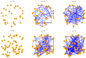
To add graphical interactions, we first generate an undirected graph. Given the number of nodes , we then randomly generate an edge between any two nodes with probability , where controls the sparsity of the edges. Figure 2 shows examples of the generated graphs for , corresponding to none, mild and dense connectivities among the nodes. Denote as a generated graph. We define as the precision matrix of the random vector . In particular, we set the element of as
where controls the partial correlation levels. Accordingly, is generated from . By this construction, has as its partial correlation graph (Dahlhaus & Eichler, 2003).
We partition the interval into an equally spaced time grid with . Under this setting, when so that the functional data is densely observed. We then generate according to (27). For the data contamination, we add an additional noise to , where is independent Gaussian random variables with mean zero and variance for each given .
4.2 Results
We use six different FPCA methods, namely, SFPCA, DFPCA, weakly-separable SFPCA (WSFPCA), weakly-separable DFPCA (WDFPCA), GSFPCA, and GDFPCA, to reconstruct the MFTS from the simulated data; see Table 1 for a detailed comparison of these methods. Particularly, SFPCA and DFPCA are the univariate FPCAs that reconstruct each individual series of the MFTS separately; see Ramsay & Silvermann (2005) and Hörmann et al. (2015) for details. WSFPCA and WDFPCA are the FPCAs based on the weakly-separable KL expansions (17) and (15), respectively. WSFPCA and WDFPCA estimate the scores as in their univariate versions, except that they combine the information from multiple individual series to estimate the eigenfunctions and functional filters; see Zapata et al. (2022) and Section 3.1 for more details.
| Representation | Literature | Scores | |
| SFPCA | Ramsay & Silvermann (2005) | ||
| WSFPCA | Zapata et al. (2022) | ||
| GSFPCA | — | Optimization | |
| DFPCA | Hörmann et al. (2015) | ||
| WDFPCA | — | ||
| GDFPCA | — | Optimization |
Moreover, GSFPCA and GDFPCA are the graphical versions of WSFPCA and WDFPCA that additionally consider graphical interactions for the score extraction. For GSFPCA and GDFPCA, we reconstruct the MFTS in the same way as WSFPCA and WDFPCA, except that we extract the scores by optimizing their conditional densities.
In addition to the aforementioned six FPCAs, we also consider two other methods, denoted as (G)SFPCA and (G)DFPCA, which are counterparts to GSFPCA and GDFPCA with the graph being known. Different from GSFPCA and GDFPCA, we set
where denotes the collection of all positive-definite matrices with the element being 0 when . This indicates that is estimated by incorporating the known graphical constraints according to Theorem 1. We use Algorithm 17.1 in Friedman et al. (2001) to obtain for the score extractions of (G)SFPCA and (G)DFPCA.
We conduct 100 simulations for each setting. To compare the reconstruction accuracy, we define the normalized mean square error using the first components:
where for WDFPCA and GDFPCA is defined as , with and selected by the ratio of variance explained and the cumulative norm, respectively; see part B.2 in Supplementary Materials for their definitions. For other static FPCAs, are defined analogously according to Table 1.
| SFPCA | 52.36 | 39.90 | 35.49 | 33.96 | 52.15 | 39.50 | 34.80 | 33.19 | 53.88 | 41.11 | 36.58 | 34.99 | ||
| WSFPCA | 64.93 | 45.35 | 30.74 | 21.50 | 64.02 | 44.30 | 29.81 | 20.52 | 63.58 | 43.71 | 30.54 | 22.47 | ||
| GSFPCA | 64.59 | 44.53 | 29.25 | 18.85 | 63.69 | 43.53 | 28.37 | 18.11 | 63.10 | 42.70 | 28.76 | 19.59 | ||
| (G)SFPCA | 64.59 | 44.53 | 29.25 | 18.84 | 63.67 | 43.48 | 28.31 | 18.06 | 62.98 | 42.48 | 28.47 | 19.28 | ||
| DFPCA | 50.26 | 39.31 | 37.05 | 36.76 | 49.99 | 38.50 | 36.00 | 35.66 | 51.39 | 40.06 | 37.75 | 37.46 | ||
| WDFPCA | 63.23 | 42.99 | 29.05 | 19.84 | 61.86 | 41.66 | 27.65 | 19.23 | 60.78 | 40.63 | 28.92 | 22.53 | ||
| GDFPCA | 63.03 | 41.81 | 25.93 | 15.06 | 61.65 | 40.16 | 24.40 | 14.13 | 59.94 | 38.17 | 24.28 | 15.82 | ||
| (G)DFPCA | 63.04 | 41.81 | 25.94 | 15.05 | 61.63 | 40.10 | 24.34 | 14.08 | 59.83 | 38.00 | 24.02 | 15.60 | ||
| SFPCA | 55.63 | 39.00 | 30.41 | 26.06 | 55.73 | 38.93 | 30.26 | 25.77 | 56.33 | 39.32 | 30.76 | 26.41 | ||
| WSFPCA | 63.92 | 42.91 | 27.53 | 17.15 | 63.32 | 42.37 | 27.22 | 16.89 | 62.56 | 41.89 | 27.07 | 17.50 | ||
| GSFPCA | 63.72 | 42.47 | 26.75 | 15.93 | 63.14 | 41.96 | 26.46 | 15.73 | 62.33 | 41.39 | 26.20 | 16.17 | ||
| (G)SFPCA | 63.72 | 42.47 | 26.75 | 15.93 | 63.11 | 41.90 | 26.38 | 15.62 | 62.23 | 41.19 | 25.92 | 15.81 | ||
| DFPCA | 50.89 | 34.31 | 28.05 | 26.29 | 50.85 | 34.11 | 27.65 | 25.75 | 51.44 | 34.61 | 28.26 | 26.45 | ||
| WDFPCA | 61.81 | 39.47 | 23.18 | 12.11 | 60.70 | 38.58 | 22.82 | 12.47 | 58.78 | 36.77 | 22.46 | 13.84 | ||
| GDFPCA | 61.69 | 38.70 | 21.58 | 9.75 | 60.57 | 37.53 | 20.82 | 9.50 | 58.36 | 35.38 | 19.84 | 10.09 | ||
| (G)DFPCA | 61.69 | 38.70 | 21.58 | 9.75 | 60.54 | 37.49 | 20.76 | 9.44 | 58.27 | 35.25 | 19.66 | 9.90 | ||
| SFPCA | 51.94 | 39.36 | 34.91 | 33.37 | 51.71 | 39.34 | 35.00 | 33.51 | 58.71 | 42.70 | 37.07 | 35.00 | ||
| WSFPCA | 64.88 | 45.08 | 30.28 | 20.96 | 64.85 | 44.74 | 30.05 | 20.86 | 62.77 | 41.84 | 32.28 | 26.79 | ||
| GSFPCA | 64.57 | 44.29 | 28.88 | 18.43 | 64.54 | 43.96 | 28.66 | 18.36 | 62.05 | 40.37 | 30.03 | 23.79 | ||
| (G)SFPCA | 64.57 | 44.29 | 28.88 | 18.43 | 64.52 | 43.92 | 28.61 | 18.33 | 61.86 | 40.00 | 29.52 | 23.17 | ||
| DFPCA | 50.07 | 38.79 | 36.43 | 36.14 | 49.81 | 38.75 | 36.48 | 36.17 | 53.15 | 39.23 | 36.41 | 36.03 | ||
| WDFPCA | 63.34 | 42.57 | 28.38 | 18.79 | 63.22 | 42.22 | 28.23 | 18.82 | 56.27 | 36.21 | 29.11 | 26.30 | ||
| GDFPCA | 63.15 | 41.68 | 25.53 | 14.53 | 63.01 | 41.25 | 25.27 | 14.48 | 54.55 | 32.34 | 23.22 | 18.68 | ||
| (G)DFPCA | 63.15 | 41.68 | 25.53 | 14.53 | 62.99 | 41.23 | 25.22 | 14.45 | 54.49 | 32.20 | 23.04 | 18.47 | ||
| SFPCA | 55.48 | 38.70 | 30.28 | 25.90 | 55.36 | 38.72 | 30.30 | 25.92 | 56.77 | 40.01 | 31.12 | 26.69 | ||
| WSFPCA | 63.62 | 42.67 | 27.36 | 16.97 | 63.47 | 42.45 | 27.25 | 16.97 | 59.19 | 38.6 | 25.46 | 17.46 | ||
| GSFPCA | 63.43 | 42.24 | 26.60 | 15.78 | 63.28 | 42.03 | 26.50 | 15.78 | 58.93 | 38.08 | 24.61 | 16.26 | ||
| (G)SFPCA | 63.43 | 42.24 | 26.60 | 15.78 | 63.26 | 41.99 | 26.44 | 15.71 | 58.79 | 37.79 | 24.16 | 15.67 | ||
| DFPCA | 50.79 | 33.96 | 27.66 | 25.84 | 50.80 | 34.13 | 27.93 | 26.15 | 51.82 | 34.80 | 28.46 | 26.66 | ||
| WDFPCA | 61.70 | 39.37 | 22.81 | 11.44 | 61.46 | 39.08 | 22.80 | 11.72 | 53.66 | 31.71 | 20.64 | 15.11 | ||
| GDFPCA | 61.58 | 38.65 | 21.50 | 9.50 | 61.34 | 38.31 | 21.32 | 9.55 | 51.94 | 28.60 | 16.22 | 9.58 | ||
| (G)DFPCA | 61.58 | 38.65 | 21.51 | 9.50 | 61.33 | 38.29 | 21.28 | 9.51 | 51.86 | 28.44 | 16.01 | 9.29 | ||
In Table 2, we present results of averaged from 100 simulations for the cases of and . The case of is also given in Part C.1 in Supplementary Materials. In each simulation, the data are generated with , and hence the optimal representation of the MFTS differs from its static representation according to Theorem 4. Consequently, the dynamic versions of FPCAs are expected to perform better than their static counterparts; this is indeed the case in our simulations for most of the combinations of , , and . Besides, for a fixed number of , the NMSEs of WDFPCA and GDFPCA become smaller as the number of time units increases. This supports our statistical properties discussed in Section 3.3. In addition, for any fixed , and , the NMSEs of the dynamic version of FPCAs are the smallest when , the true truncation number in (27). Recall that when calculating , we use the first components. In our simulation, we always find . For this reason, we only report results up to .
In Part C.1 of Supplementary Materials, we present the variances of the estimated functional filters by different dynamic FPCAs. We discover that the variances of the estimated functional filters from WDFPCA or GDFPCA are significantly smaller than those from DFPCA. These findings provide supporting evidences for Theorem 6 and also explain the results in Table 2, where the averaged values of the DFPCA are significantly larger than those of the other dynamic FPCAs when . Furthermore, we find that GDFPCA always outperforms WDFPCA, and the improvement is more significant when and . In these cases, the functions across different individuals may be highly correlated, and we need to further account for these graphical interactions for score extractions as there is limited information at the temporal level.
Overall, GDFPCA can borrow strength across different individual series in the graph, thereby reducing estimation errors for both functional filters and scores when is relatively small. Moreover, note that the performances of GDFPCA are nearly identical to those of (G)DFPCA, respectively, indicating that our proposed joint graphical Lasso estimator for works well for our purpose.
| Case 1 | Case 2 | ||||||
| SFPCA | 33.32 | 33.25 | 33.64 | 6.11 | 5.86 | 6.45 | |
| WSFPCA | 24.71 | 24.80 | 24.98 | 5.51 | 5.28 | 5.85 | |
| GSFPCA | 23.62 | 23.72 | 23.74 | 4.68 | 4.50 | 4.94 | |
| DFPCA | 32.83 | 32.69 | 33.35 | 11.24 | 10.77 | 11.61 | |
| WDFPCA | 16.82 | 18.47 | 19.30 | 7.59 | 7.51 | 8.42 | |
| GDFPCA | 13.82 | 15.22 | 15.33 | 4.84 | 4.67 | 5.16 | |
| SFPCA | 33.36 | 33.87 | 32.17 | 6.00 | 6.05 | 6.43 | |
| WSFPCA | 24.63 | 24.91 | 26.76 | 5.39 | 5.41 | 5.85 | |
| GSFPCA | 23.57 | 23.85 | 26.22 | 4.59 | 4.61 | 4.89 | |
| DFPCA | 33.11 | 34.05 | 30.93 | 10.95 | 11.04 | 11.50 | |
| WDFPCA | 17.09 | 17.30 | 22.68 | 7.34 | 7.29 | 8.78 | |
| GDFPCA | 14.05 | 14.43 | 17.58 | 4.72 | 4.73 | 4.75 | |
To further investigate the robustness of the dynamic weak separability (4), we conduct additional simulations for the cases that the dynamic weak separability (4) is not satisfied (case 1) or degenerates to the weak separability (5) (case 2). For case 1, we generate the data by (27), except that we multiply a fluctuation to for each . For case 2, we simply set in (27) for the data generation. This time we only report results for and . When the dynamic weak separability (4) is not satisfied, the GDFPCA may not be the optimal choice for the reconstruction of MFTS. Nonetheless, Table 3 (case 1) shows that the reconstruction by GDFPCA still performs competitively, owing to its lower estimation uncertainty by pooling together data from different nodes.
When , the dynamic weak separability (4) still holds, but it degenerates to the weak separability (5). We investigate this case (case 2 in Table 3) to compare the performance of FPCAs. Results show that the static FPCAs outperform their dynamic counterparts in most cases, which is expected based on Theorem 4. Normally, the dynamic representation has higher model complexity than its static counterpart, which may result in a poorer reconstruction under a simpler dependence structure. Nevertheless, unlike the DFPCA and WDFPCA, the results of GDFPCA are satisfactory compared with those of their static counterparts. This finding suggests that considering graphical interactions for score extractions may alleviate model complexities raised by the dynamic representation.
5 Data Illustration
For data analysis, we consider hourly readings of PM2.5 concentration (measured in ) collected from 24 monitoring stations (in three cities in China) in the winter of 2016, with a total length of 60 days. A square-root transformation is employed to stabilize the variance. Then in our notation, we observe a discrete MFTS with , , and . Examples of daily curves and locations of monitoring stations are illustrated in Figure 1.
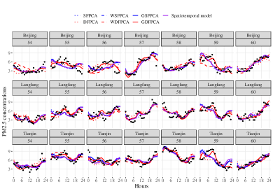
We respectively apply the FPCAs in Table 1 to reconstruct the MFTS. For these FPCAs, we choose their truncation numbers or in Table 1 using the fractions of variance explained (FVE), with the FVE set to be larger than 80%; the definitions of FVE can be found in Part B.2 in Supplementary Materials. In our case, takes different values for SFPCA and DFPCA, and for WSFPCA, GSFPCA, WDFPCA and GDFPCA. Besides, or in Table 1 are determined similarly as in Section 4. In addition to the FPCA approaches, we also compare a spatiotemporal model similar to the GSFPCA. This model was proposed by Wikle et al. (2019), where they denote as , and the spatiotemporal responses are approximated using . Here, , and are the same as in GSFPCA, is the geographical location of a station, and is a zero-mean Gaussian process with stationary exponential covariance function for each pair . For each , we estimate by their conditional expectations onto utilizing the geographical information of stations; see Section 4.4.3 of Wikle et al. (2019) for more details.
For illustration, we separately pick one station from each city and show the reconstructed MFTS for the last seven days of the study period in Figure 3. One can see that the reconstructed MFTS using DFPCA and WDFPCA performs poorly in capturing the data pattern due to their biases for the scores at the boundaries. Nonetheless, the proposed GDFPCA can better capture the curvature of data. For example, on day 59 in all three cities, there was a temporary rise followed by a big drop of PM2.5 around noon. The reconstructed curves by our method (solid red line) give the best recognition of this pattern among the methods in Figure 3.
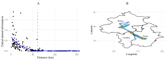
Unlike the above spatiotemporal model, we do not assume the spatial stationarity condition for the MFTS data; therefore, our proposed GDFPCA is more flexible in capturing spatial dependencies within the temporally correlated functions. To characterize the spatial dependencies, we utilize the partial mutual information (Brillinger, 1996) for multivariate time series, which is defined as
where is the joint graphical Lasso estimator in Section 3.1. In Figure 4 A, we present a scatter plot of the partial mutual information for all pairs of stations versus their geographical distances. It shows that tends to decrease if the distance between stations and gets large. When the distance is larger than km ( of all pairs), the partial mutual information is almost zero. That means, the connectivity among these stations can be ignored. In Figure 4 B, we present a partial correlation graph for station pairs by calculating their partial mutual information, with a thresholding value for taken as 0.05. As shown in Figure 4 B, we find that the PM2.5 concentration among the stations in Tianjin and Langfang is more partially correlated.
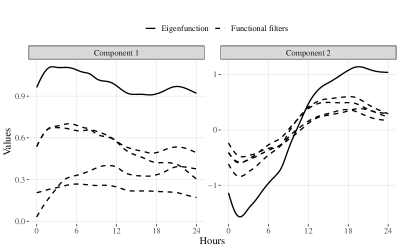
In Part C.2 in Supplementary Materials, we illustrate the validity of the dynamic weak separability (4) for the PM2.5 data. To further evaluate the static and dynamic representations, we investigate the covariance structures via the estimated eigenfunctions and functional filters. Note that in general, the functional filter cannot be uniquely identified, unless the weak separability (5) is satisfied. In that case, , , are proportional to each other for each , and the dynamic FPCA degenerates to its static counterpart according to Theorem 4. We compare the eigenfunctions and functional filters of the first two components obtained from GSFPCA and GDFPCA in Figure 5. It shows that the eigenfunctions and functional filters are quite different in shape. This finding suggests that the separability condition (5) is not satisfied. Thus, using dynamic FPCAs to reconstruct the underlying MFTS would be more appropriate for the PM2.5 data.
6 Discussion
In this study, we develop a theoretical framework to model and reconstruct MFTS from noisy data, considering both serial dependencies and graphical interactions. These two-way dependencies may lead to inefficient dimension reduction when using classical FPCA methods. We propose a key assumption of dynamic weak separability (4), under which we define the partial correlation graph for infinite-dimensional MFTS and facilitate the DFPCA (Hörmann et al., 2015) to optimally reconstruct signals of MFTS by using graphical-level information. The superior performance of GDFPCA has been demonstrated through a series of simulation studies and a real data example.
Weak separability (Lynch & Chen, 2018; Liang et al., 2023) is a novel concept for functional data to characterize the covariance structure among random curves. According to our theories and simulation study, the form of weak separability plays a prominent role in both defining graphical models and determining optimal approximations. Notably, under the dynamic weak separability condition, we establish a valid partial spectral density kernel to evaluate the partial correlation graph among infinite-dimensional curves. While the theoretical framework in Zapata et al. (2022) is only applicable for independently sampled curves, we relax this sampling scheme to weakly dependent functional time series. Since the scores obtained from the proposed GDFPCA preserve all the graph information, a potential application of our method can be forecasts of functional time series by borrowing strength from other curves in the graph.
To reconstruct the MFTS by the GDFPCA, we follow the joint graphical Lasso method proposed by Danaher et al. (2014) to estimate , rather than estimating the actual graph . These are essentially two different topics. Through empirical studies, we have found that the estimated is not sensitive to the reconstruction results, and thus the algorithm proposed in Section 3.1 is sufficient for dimension reduction. Alternatively, if the study goal is to reveal the actual graph, one may estimate edges using from (16). To do that, a more sophisticated model selection method may be necessary since the errors from estimating edges and the selection of the finite truncation may significantly influence the resulting graph. In Zapata et al. (2022), the unknown graph for independently sampled multivariate functional data was estimated by a modified joint graphical Lasso, where the penalty term was designed to regularize both the sparsity level for each and the common sparsity levels shared by . Under our framework, a similar procedure can be potentially developed based on the penalized likelihood (22).
References
- (1)
- Boyd et al. (2011) Boyd, S., Parikh, N., Chu, E., Peleato, B., Eckstein, J. et al. (2011), ‘Distributed optimization and statistical learning via the alternating direction method of multipliers’, Foundations and Trends® in Machine learning 3(1), 1–122.
- Brillinger (1996) Brillinger, D. R. (1996), ‘Remarks concerning graphical models for time series and point processes’, Brazilian Review of Econometrics 16(1), 1–23.
- Brillinger, David R (2001) Brillinger, David R (2001), Time series: data analysis and theory, SIAM.
- Chen et al. (2017) Chen, K., Delicado, P. & Müller, H.-G. (2017), ‘Modelling function-valued stochastic processes, with applications to fertility dynamics’, Journal of the Royal Statistical Society: Series B (Statistical Methodology) 79(1), 177–196.
- Chiou et al. (2014) Chiou, J.-M., Chen, Y.-T. & Yang, Y.-F. (2014), ‘Multivariate functional principal component analysis: A normalization approach’, Statistica Sinica 24(4), 1571–1596.
- Dahlhaus (2000) Dahlhaus, R. (2000), ‘Graphical interaction models for multivariate time series 1’, Metrika 51(2), 157–172.
- Dahlhaus & Eichler (2003) Dahlhaus, R. & Eichler, M. (2003), ‘Causality and graphical models in time series analysis’, Oxford Statistical Science Series pp. 115–137.
- Danaher et al. (2014) Danaher, P., Wang, P. & Witten, D. M. (2014), ‘The joint graphical lasso for inverse covariance estimation across multiple classes’, Journal of the Royal Statistical Society: Series B (Statistical Methodology) 76(2), 373–397.
- De Vito et al. (2013) De Vito, E., Umanità, V. & Villa, S. (2013), ‘An extension of mercer theorem to matrix-valued measurable kernels’, Applied and Computational Harmonic Analysis 34(3), 339–351.
- Dunsmuir (1979) Dunsmuir, W. (1979), ‘A central limit theorem for parameter estimation in stationary vector time series and its application to models for a signal observed with noise’, The Annals of Statistics 7(3), 490–506.
- Epskamp & Fried (2018) Epskamp, S. & Fried, E. I. (2018), ‘A tutorial on regularized partial correlation networks.’, Psychological methods 23(4), 617.
- Friedman et al. (2001) Friedman, J., Hastie, T., Tibshirani, R. et al. (2001), The elements of statistical learning, Vol. 1, Springer series in statistics New York.
- Gao & Shang (2017) Gao, Y. & Shang, H. L. (2017), ‘Multivariate functional time series forecasting: Application to age-specific mortality rates’, Risks 5(2), 21.
- Gao et al. (2019) Gao, Y., Shang, H. L. & Yang, Y. (2019), ‘High-dimensional functional time series forecasting: An application to age-specific mortality rates’, Journal of Multivariate Analysis 170, 232–243.
- Hörmann et al. (2015) Hörmann, S., Kidziński, Ł. & Hallin, M. (2015), ‘Dynamic functional principal components’, Journal of the Royal Statistical Society: Series B (Statistical Methodology) 77(2), 319–348.
- Hörmann & Kokoszka (2010) Hörmann, S. & Kokoszka, P. (2010), ‘Weakly dependent functional data’, The Annals of Statistics 38(3), 1845–1884.
- Hsing & Eubank (2015) Hsing, T. & Eubank, R. (2015), Theoretical foundations of functional data analysis, with an introduction to linear operators, Vol. 997, John Wiley & Sons.
- James et al. (2000) James, G. M., Hastie, T. J. & Sugar, C. A. (2000), ‘Principal component models for sparse functional data’, Biometrika 87(3), 587–602.
- Jung et al. (2015) Jung, A., Hannak, G. & Goertz, N. (2015), ‘Graphical lasso based model selection for time series’, IEEE Signal Processing Letters 22(10), 1781–1785.
- Liang et al. (2023) Liang, D., Huang, H., Guan, Y. & Yao, F. (2023), ‘Test of weak separability for spatially stationary functional field’, Journal of the American Statistical Association 118(543), 1606–1619.
- Lynch & Chen (2018) Lynch, B. & Chen, K. (2018), ‘A test of weak separability for multi-way functional data, with application to brain connectivity studies’, Biometrika 105(4), 815–831.
- Mateu & Giraldo (2021) Mateu, J. & Giraldo, R. (2021), Geostatistical Functional Data Analysis, John Wiley & Sons.
- Qiao et al. (2019) Qiao, X., Guo, S. & James, G. M. (2019), ‘Functional graphical models’, Journal of the American Statistical Association 114(525), 211–222.
- Qiao et al. (2020) Qiao, X., Qian, C., James, G. M. & Guo, S. (2020), ‘Doubly functional graphical models in high dimensions’, Biometrika 107(2), 415–431.
- Ramsay & Silvermann (2005) Ramsay, J. & Silvermann, B. (2005), ‘Functional data analysis. springer series in statistics’.
- Whittle (1961) Whittle, P. (1961), ‘Gaussian estimation in stationary time seris’, Bull. Internat. Statist. Inst. 39, 105–129.
- Wikle et al. (2019) Wikle, C. K., Zammit-Mangion, A. & Cressie, N. (2019), Spatio-temporal Statistics with R, Chapman and Hall/CRC.
- Yao et al. (2005) Yao, F., Müller, H.-G. & Wang, J.-L. (2005), ‘Functional data analysis for sparse longitudinal data’, Journal of the American statistical association 100(470), 577–590.
- Zapata et al. (2022) Zapata, J., Oh, S.-Y. & Petersen, A. (2022), ‘Partial separability and functional graphical models for multivariate gaussian processes’, Biometrika 109(3), 665–681.
- Zhu et al. (2022) Zhu, X., Cai, Z. & Ma, Y. (2022), ‘Network functional varying coefficient model’, Journal of the American Statistical Association 117(540), 2074–2085.