Shear Alfvénic Waves in Electron-Positron Plasma: Analysis of Solitary Wave Properties and Numerical Validation

Abstract

The investigation employed the reductive perturbation approach to study the nonlinear propagation of shear Alfvénic waves in an electron-positron (EP) plasma medium. Utilizing the solitary wave solution of the derivative nonlinear Schrödinger equation, the fundamental properties of EP shear Alfvén (EPSA) waves were identified, with a focus on their key features such as speed, amplitude, and width. The analysis revealed the presence of hump-shaped solitary waves. Additionally, comparing the numerical results obtained through the finite difference method and the exact solution demonstrated good agreement between the two. These findings hold significance in comprehending nonlinear electromagnetic wave phenomena in laboratory plasma and space environments where EP plasma is present such as solar wind, Earth’s magnetosphere, pulsars’ magnetospheres, microquasars, and tokamaks.

I Introduction

Electron-positron (EP) plasmas are observed in diverse astrophysical contexts, including the solar wind Clem2000 ; Adriani2009 ; Adriani2011 , Earth’s magnetosphere Ackermann2012 ; Aguilar2014 , pulsars’ magnetospheres Profumo2012 , and microquasars Siegert2016 . In laboratory settings, EP plasmas can be generated through ultra-intense laser-matter interactions Sarri2013 ; Sarri2015 . Strong magnetic/electric fields or extremely high temperatures also contribute to EP plasma creation Thoma2009 , with advancements in assembling pure positron plasmas in Penning traps Greaves1994 ; Surko1989 . The occurrence of EP pair production is anticipated in post-disruption plasmas in large tokamaks Helander2003 . Notably, the physics of EP plasmas differs significantly from electron-ion plasmas due to the large ion-to-electron mass ratio Swanson2003 ; Stix1992 . EP plasmas in the vicinity of magnetars and fast-rotating neutron stars experience strong magnetic fields, with similar conditions replicable in intense laser-plasma interaction experiments. Consequently, the study of collective phenomena in magnetized pair plasmas has garnered substantial interest Zank1995 ; Iwamoto1993 ; Lominadze1982 ; Gedalin1985 ; Yu1986 ; Brodin2007 ; Rajib2015 ; Rajib2022a ; Rajib2022b .

Extensive theoretical and numerical investigations have elucidated the distinctive physics of EP plasmas, covering fundamental wave physics Zank1995 , reconnection Bessho2005 ; Blackman1994 ; Yin2008 , and nonlinear solitary waves Berezhiani1994 ; Cattaert2005 . Sakai and Kawata Sakai1980 analyzed small-amplitude solitary waves using higher-order modified Korteweg-de Vries (mK-dV) equations from relativistic hydrodynamic equations, while Zank and Greaves Zank1995 explored linear properties of electrostatic and electromagnetic modes in both unmagnetized and magnetized pair plasmas. El-Wakil et al. Elwakil2019 investigated solitary wave propagation in EP pair plasmas using reductive perturbation theory and nonlinear equations. Iwamoto Iwamoto1993 provided a kinetic description of various linear collective modes in a non-relativistic pair magnetoplasma, and Helander and Ward Helander2003 demonstrated positron creation in tokamaks due to collisions of runaway electrons with plasma ions/thermal electrons. Lontano et al. Lontano2001 studied the interaction between arbitrary amplitude electromagnetic fields and EP (hot) plasma. The nonlinear wave propagation of EP plasma in a pulsar magnetosphere was investigated by Kennel et al. Kennel1976 ; Arons1986 , who observed that large amplitude waves determine average plasma properties.

Shear Alfvén (SA) waves are magnetohydrodynamic waves in magnetized plasmas that propagate in the direction of the ambient magnetic field, and the motion of the plasma particles (here EP) and the perturbation of the magnetic field are transverse to the direction of propagation. Observations of SA waves have been documented in numerous laboratory experiments Gekelman1999 and occur naturally in a diverse range of astrophysical magnetized plasmas, including planetary magnetospheres Pater2001 , Earth’s aurora Louarn1994 , solar corona Hollweg1982 , and more. Due to their propagation primarily along an ambient magnetic field Hasegawa1976 ; Goertz1979 ; Gekelman1997 , SA wave demonstrates efficient energy transport. Various theoretical studies Sakai1980 ; Melikidze1981 ; Stenflo1985 have explored nonlinear Alfvén wave propagation in EP plasmas. Melikidze et al. Melikidze1981 analyzed solitary wave properties for field-aligned electromagnetic waves, while Stenflo et al. Stenflo1985 considered Alfvén waves in a cold electron-positron plasma, describing the coupling of radiation with cold electrostatic oscillations. Mikhailovskii et al. Mikhailovskii1985 theoretically examined nonlinear Alfvén waves in a relativistic EP plasma.

In addition to opposite polarity EP pair plasmas, recent theoretical predictions and observational data from satellites and experiments have prompted several authors D'Angelo2001 ; D'Angelo2002 ; Shukla2006 ; Mamun2002 ; Sayed2007 ; Rahman2008 ; Mamun2008a ; Mamun2008b ; Verheest2009 to explore dusty plasmas featuring dust particles with opposite polarity. These studies have delved into both linear D'Angelo2001 ; D'Angelo2002 ; Shukla2006 and nonlinear Mamun2002 ; Sayed2007 ; Rahman2008 ; Mamun2008a ; Mamun2008b ; Verheest2009 electrostatic waves, with investigations conducted both in the absence D'Angelo2001 ; Shukla2006 ; Mamun2002 ; Sayed2007 ; Rahman2008 ; Mamun2008a ; Mamun2008b ; Verheest2009 and presence D'Angelo2002 of an external static magnetic field. Moreover, Shukla Shukla2004 and Mamun Mamun2011 have explored a medium composed of magnetized dust particles with opposite polarity to investigate both linear and nonlinear electromagnetic waves. Shukla’s analytical work focused on linear dispersive dust Alfvén waves and associated dipolar vortices Shukla2004 , while Mamun’s research delved into the nonlinear propagation of fast and slow dust magnetoacoustic modes Mamun2011 .

In a prior study Mamun2013 , Mamun explored shear Alfvénic solitary structures within an opposing polarity dusty plasma medium, noting the applicability of this plasma model to various scenarios, including EP and electron-ion plasmas. This current research builds upon the earlier work Mamun2013 , specifically focusing on the extension of the study when the ratio of positron mass to electron mass is set to unity, denoted by $\alpha=m_{p}/m_{e}=1$. In our present investigation, we delve into the realm of EP plasma, conducting a systematic analysis of high-frequency nonlinear shear Alfvén solitary waves through the utilization of the well-established derivative nonlinear Schrödinger equation (DNSE) coupled with the reductive perturbation technique.

The manuscript is structured as follows: Section II provides the governing equations outlining our plasma model and a concise explanation of the mathematical technique, followed by the derivation of a DNSE along with its solution. Section III presents the numerical analysis and results, and lastly, Section IV concludes with a discussion.

II Governing Equations

We consider collisionless, magnetized ultra-high frequency electromagnetic perturbations in a medium of EP, which is assumed to be immersed in an external static magnetic field $\vec{B}_{0}$ (i.e., $\vec{B}_{0}$$||$$\hat{z}$, where $\hat{z}=$ unit vector along the z-axis). Thus, the macroscopic state of the medium of opposite polarity magnetized EP fluids D'Angelo2002 ; Shukla2004 ; Mamun2011 is described by the following set of equations

$$\hskip 14.22636pt{\partial_{t}}N_{s}+{\partial_{z}}(N_{s}{U}_{sz})=0,$$ (1)

$$\hskip 14.22636ptm_{s}D_{t}^{s}{\vec{U}}_{s}=q_{s}\left({\vec{E}}+\frac{1}{c}{\vec{U}}_{s}\times{\vec{B}}\right),$$ (2)

$$\hskip 14.22636pt{\hat{z}}\times\partial_{z}{\vec{E}}=-\frac{1}{c}{\partial_{t}{\vec{B}}},$$ (3)

$$\hskip 14.22636pt{\hat{z}}\times\partial_{z}{\vec{B}}=\frac{4\pi}{c}\sum_{s}q_{s}N_{s}{\vec{U}}_{s},$$ (4)

$$\hskip 14.22636pt\partial_{z}{\vec{B}}=0,$$ (5)

$$\hskip 14.22636pt0=4\pi\sum_{s}q_{s}N_{s},$$ (6)

where $D_{t}^{s}=\partial_{t}+U_{sz}\partial_{z}$, $\partial_{z}={\partial}/{\partial_{z}}$ and $\partial_{t}={\partial}/{\partial_{t}}$ $s~{}(=e,p)$ denotes the species (namely, electron and positron); $m_{s}$, $q_{s}$, and $N_{s}$ are, respectively, mass, charge, and number density of the species $s$; ${\vec{U}}_{s}$ is the hydrodynamic velocity; ${\vec{E}}$ is the electromagnetic wave electric field, and ${\vec{B}}$ is the sum of external and wave magnetic fields; $c~{}(=3\times 10^{8}~{}m/s)$ is the speed of light in a vacuum.

Now, neglecting the contribution of the displacement current as of the wave phase speed is negligible compared to the speed of light $c$ and assuming the quasi-neutrality condition ($N_{e}=N_{p}$), we can reduce our basic equations (1)$-$(6) to

$${\partial_{t}}N_{s}+{\partial_{z}}(N_{s}{U}_{sz})=0,$$ (7)

$$N_{s}D_{t}^{s}\left[(1+\alpha){U}_{sx}-{{\alpha}{\cal H}({\partial_{z}}B_{y}})\right]-b{{\partial_{z}}B_{x}}=0,$$ (8)

$$N_{s}D_{t}^{s}\left[(1+\alpha){U}_{sy}+{{\alpha}{\cal H}({\partial_{z}}B_{x}})\right]-b{{\partial_{z}}B_{y}}=0,$$ (9)

$$N_{s}D_{t}^{s}(1+\alpha){\vec{U}}_{sz}+\frac{b}{B_{0}}(B_{y}{{\partial_{z}}B_{y}}+B_{x}{{\partial_{z}}B_{x}})=0,$$ (10)

$${\partial_{t}B_{x}}-\partial_{z}(U_{sx}B_{0}-U_{sz}B_{x})+\frac{B_{0}}{\omega_{cs}}\partial_{z}D_{t}^{s}U_{sy}=0,$$ (11)

$${\partial_{t}B_{y}}-\partial_{z}(U_{sy}B_{0}-U_{sz}B_{y})-\frac{B_{0}}{\omega_{cs}}\partial_{z}D_{t}^{s}U_{sx}=0,$$ (12)

where $B_{z}=B_{0}$, $\omega_{cs}=q_{s}B_{0}/m_{s}c$, $V_{As}=B_{0}/\sqrt{4\pi N_{s0}m_{s}}$, $b=V_{As}^{2}N_{s0}/B_{0}$, ${\cal H}=b/{\omega_{cs}N_{s}}$, $\alpha=m_{p}/m_{e}=1$ (Note that we consider $\alpha$ is equal to unity on the rest of the manuscript for our considered system as the mass of electron and positron is same).

We are interested in high-frequency small but finite amplitude electromagnetic perturbation modes propagating along the $z$-axis (i.e., all dependent variables depend on $z$ and $t$ only) in the presence of an external static magnetic field ${\vec{B}}_{0}$ that are exactly parallet $\theta$ with the $z$-axis (i.e., $\theta=0^{\circ}$). We construct a weakly nonlinear theory which leads to the following stretched coordinates Washimi1966 ; Haider2019

$$\left.\begin{array}[]{l}\xi=\epsilon(z-V_{p}t),\\ \tau=\epsilon^{2}t,\end{array}\right\}$$ (15)

where $V_{p}$ is the phase speed of the EPSA waves and $\epsilon$ $(0<\epsilon<1)$ is a small parameter measuring the weakness of the dispersion. We then expand the dependent variables $N_{s}$, $U_{sx}$, $U_{sy}$, $U_{sz}$, $B_{x}$, and $B_{y}$ (where the subscript $x$, $y$, and $z$, respectively, represent $x$-, $y$- and $z$-components of the quantity involved) about their equilibrium values in powers of $\epsilon$:

$$\left.\begin{array}[]{l}N_{s}=1+\epsilon N_{s}^{(1)}+\epsilon^{2}N_{s}^{(2)}+\cdot\cdot\cdot,\\ U_{sx}=0+\epsilon^{1/2}U^{(1)}_{sx}+\epsilon^{3/2}U_{sx}^{(2)}+\cdot\cdot\cdot,\\ U_{sy}=0+\epsilon^{1/2}U_{sy}^{(1)}+\epsilon^{3/2}U_{sy}^{(2)}+\cdot\cdot\cdot,\\ U_{sz}=0+\epsilon U^{(1)}_{sz}+\epsilon^{2}U_{sz}^{(2)}+\cdot\cdot\cdot,\\ B_{x}=0+\epsilon^{1/2}B^{(1)}_{x}+\epsilon^{3/2}B_{x}^{(2)}+\cdot\cdot\cdot,\\ B_{y}=0+\epsilon^{1/2}B^{(1)}_{y}+\epsilon^{3/2}B_{y}^{(2)}+\cdot\cdot\cdot,\\ \end{array}\right\}$$ (22)

Now, substituting the above-stretched co-ordinates (15) and expansion series into equations (8), (9), (11), and (12) and equating the coefficients of $\epsilon^{3/2}$ we obtain a set of equations that can be simplified as

$$U^{(1)}_{sx}=-V_{p}B_{x}^{(1)}/B_{0},$$ (23)

$$U^{(1)}_{sy}=-V_{p}B_{y}^{(1)}/B_{0},$$ (24)

$$B^{(1)}_{x}=-2V_{p}B_{0}U^{(1)}_{sx}/V^{2}_{As},$$ (25)

$$B^{(1)}_{y}=-2V_{p}B_{0}U^{(1)}_{sy}/V^{2}_{As},\$$ (26)

We now put $U^{(1)}_{sx}$ into the expression for $B^{(1)}_{x}$ or $U^{(1)}_{sy}$ into the expression for $B^{(1)}_{y}$, and obtain the linear dispersion relation:

$$V_{p}=V_{As}/{\sqrt{2}}=V_{A},\$$ (27)

where $V_{A}={B_{0}}/{\sqrt{4\pi(m_{e}N_{e0}+m_{p}N_{p0})}}$ represents the effective EPSA speed. Equation (27) represents the general linear dispersion relation which represents the ultra-high frequency EPSA waves, where magnetic pressure $P_{B}=B_{0}^{2}/4\pi$ gives rise to the restoring force, and the net EP mass density $\rho_{T}={m_{e}N_{e0}+m_{p}N_{p0}}$ provides the inertia.

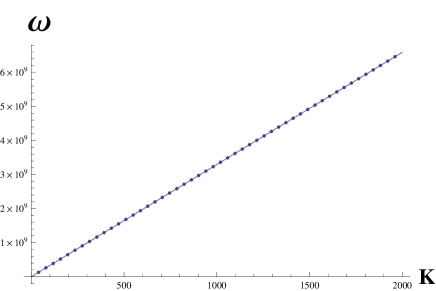
Figure 1: Showing the variation of the wave frequency $\omega$ versus wavenumber $K$

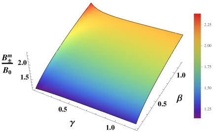
Figure 2: Showing the variation of the maximum normalized amplitude ${{B}_{\pm}^{m}}/{B_{0}}$ of EPSA soliton with $\gamma$ and $\beta$

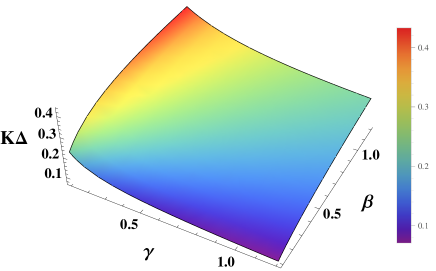
Figure 3: Showing the variation of the normalized width $K\Delta$ of EPSA soliton with $\gamma$ and $\beta$

Now, substituting equation (15) into equations (7) and (10), and equating the coefficients of $\epsilon^{2}$, we obtain

$$\hskip 42.67912ptU_{sz}^{(1)}=V_{A}|{B}_{\pm}|^{2}/2B^{2}_{0},$$ (28)

$$\hskip 42.67912ptN_{s}^{(1)}=N_{s0}|{B}_{\pm}|^{2}/2B^{2}_{0},$$ (29)

where ${B}_{\pm}=B_{y}^{(1)}\pm iB_{x}^{(1)}$ and $-$($+$) sign represents the left-hand (right-hand) circularly polarized EPSA waves. Again, as before, substitution of equation (15) in equations (8) and (9) and (11) and (12), and equating the coefficients of $\epsilon^{5/2}$, we get another set of equations. Now, one can eliminate $B_{x}^{(2)}$, $B_{y}^{(2)}$, $U_{sx}^{(2)}$, $U_{sy}^{(2)}$ and obtain

$$2\partial_{\tau}B_{x}^{(1)}+\frac{V^{2}_{A}}{\omega_{cs}}\partial_{\xi}^{2}B_{x}^{(1)}+\frac{V_{A}}{2B_{0}^{2}}\partial_{\xi}[|{B}_{\pm}|^{2}B_{y}^{(1)}]=0,$$ (30)

$$2\partial_{\tau}B_{y}^{(1)}-\frac{V^{2}_{A}}{\omega_{cs}}\partial_{\xi}^{2}B_{y}^{(1)}+\frac{V_{A}}{2B_{0}^{2}}\partial_{\xi}[|{B}_{\pm}|^{2}B_{x}^{(1)}]=0,$$ (31)

Multiplying equation (31) by $\pm i$ then adding with equation (30) allows us to write

$$i\partial_{\tau}{B}_{\pm}\pm\frac{V_{A}^{2}}{2\omega_{cs}}\partial_{\xi}^{2}{B}_{\pm}+i\frac{V_{A}\ }{4B_{0}^{2}}\partial_{\xi}[|{B}_{\pm}|^{2}{B}_{\pm}]=0,$$ (32)

where $\partial_{\xi}[|{B}_{\pm}|^{2}{B}_{\pm}]$ is called derivative nonlinear term. Equation (32) is the well-known derivative nonlinear Schrödinger equation, which describes the nonlinear propagation of the high-frequency EPSA wave in a magnetized electron-positron plasma. It is possible to get above DNSE when higher-order physical variables are included in the dynamics of wave packets as well as for exact parallel propagation of right or left-handed polarized Alfvén waves. For obliquely propagating waves, one may derive a general form of cubic nonlinear Schrödinger equation Rajib2015 .

To solve the DNSE in (32), we first normalize it by transforming the dependent and independent variables as follows

$$\left.\begin{array}[]{l}{B}_{\pm}=2B_{0}\Psi_{\pm},\\ \xi=\frac{V_{A}}{2\omega_{cs}}\zeta,\\ T=\frac{\tau}{2\omega_{cs}}.\end{array}\right\}$$ (36)

These transformations of the dependent and independent variables allow us to rewrite the DNSE (32) in the form

$$i\partial_{T}\Psi_{\pm}\pm\partial_{\zeta}^{2}\Psi_{\pm}+i\partial_{\zeta}[|\Psi_{\pm}|^{2}\Psi_{\pm}]=0,$$ (37)

where ${\partial}_{T}={\partial}/{\partial}T$ and ${\partial}_{\zeta}={\partial}/{\partial\zeta}$ and $-(+)$ sign in front of the 2nd term of (37) is for left (right) handed circularly polarized EPSA waves.

To obtain the stationary solitonic solution of the DNSE (37), we consider a traveling co-ordinate $X=\zeta{\pm}V_{0}T$, where $V_{0}$ is the wave phase speed normalized by $V_{A}$ and $X$ is normalized by $(\frac{V_{A}}{2\omega_{cs}})$. We, now apply the appropriate boundary conditions, viz. $\Psi_{\pm}(X)\rightarrow 0$, $d\Psi_{\pm}(X)/dX\rightarrow 0$, and $d^{2}\Psi_{\pm}(X)/dX^{2}\rightarrow 0$ at $X\rightarrow\pm\infty$, and use the basic property of complex variable $\Psi_{-}\Psi_{-}^{\ast}=\Psi_{+}\Psi_{+}^{\ast}=|\Psi_{\pm}|^{2}$.

The magnitude of the wave magnetic field ${B}_{\pm}$ (dimensional, where $|\Psi_{\pm}|$ is the normalized quantity), the amplitude ${B}_{\pm}^{m}$ (dimensional, where $\Psi_{\pm}(X=0)$ is the normalized quantity) and the width $\Delta$ (in dimensional form) are given by Ichikawa1979 ; Horton1996

$$\hskip 19.91692pt{B}_{\pm}=2B_{0}\sqrt{\left[\frac{(1+\Gamma)\sqrt{2\beta}}{(\sqrt{1+2\Gamma})\cosh(X/\Delta)+\sqrt{\Gamma}}\right]},$$ (38)

$$\hskip 19.91692pt{B}_{\pm}^{m}=2B_{0}\sqrt{\left[\frac{(1+\Gamma)\sqrt{2\beta}}{\sqrt{1+2\Gamma}+\sqrt{\Gamma}}\right]},$$ (39)

$$\hskip 19.91692pt\Delta=\frac{1}{2K}\sqrt{\left(\frac{\Gamma}{1+\Gamma}\right)},$$ (40)

where $\Gamma=\beta/4\gamma$, $\beta=\Omega/\omega_{cs}$, $\gamma=V_{0}/V_{A}$, and $X$ is the dimensional space variable. We note that $K=2\pi/\lambda$ and $\Omega=KV_{0}$ are used in (38)-(40), where $\lambda$ ($\Omega$) is the angular frequency dependent wavelength of the EPSA waves.

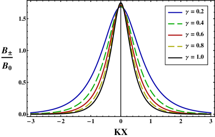
Figure 4: Showing the solitary profile of EPSA waves along with the variation of $\gamma$ with $\beta=0.5$

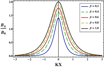
Figure 5: Showing the solitary profile of EPSA waves along with the variation of $\beta$ with $\gamma=0.5$

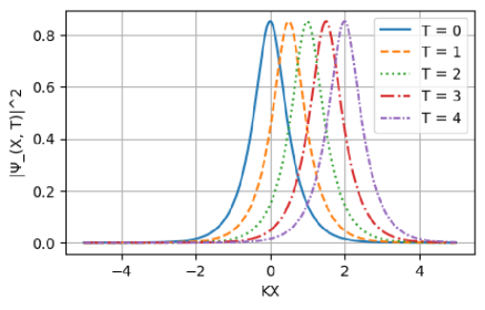
(a)

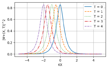
(b)

Figure 6: Time evolution of the (a) left-handed, and (b) right-handed circularly polarized EPSA solitons with $\beta=0.5$, $\gamma=0.5$, $V_{0}=0.5$, $K=1$, spatial grid spacing=0.0001, and time-step=0.01

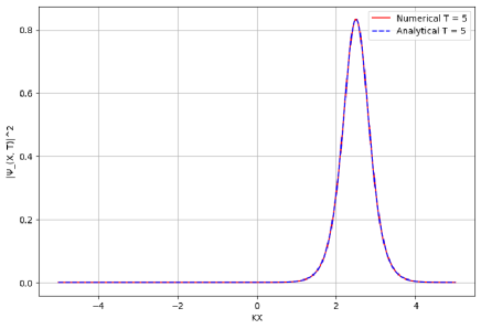
(a)

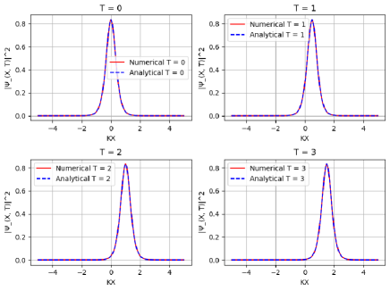
(b)

Figure 7: Comparison of analytical and numerical solutions of DNSE (37) at (a) T=5 and (b) T=0,1,2,3 with $\beta=0.5$, $\gamma=0.5$, $V_{0}=0.5$, $K=1$, spatial grid spacing=0.0001, and time-step=0.01 for left-handed circulary polarized EPSA waves

III Results and Discussion

We consider the propagation of electromagnetic perturbations in a pair EP plasma medium of opposite polarity of the same mass. We have analyzed the dispersion relation, maximum height, width, and solitary profile as well as compared it with the numerically solved solution in EPSA waves. For the numerical appreciation of the exact equation (38)-(40), we consider a crab pulsar medium with EP plasma existing for external magnetic field $B_{0}$, mass density (approx.) $\rho_{T}$, and corresponding number density $N_{s0}=\rho_{T}/2m_{s}$ Haider2012

Table 1: $B_{0}$, $\rho_{T}$, and $N_{s0}$ IN CRAB PULSAR MEDIUM

Parameters		$~{}~{}Numerical~{}~{}Value$	$Unit$	$Ref.$
$B_{0}$		$3.7\times 10^{12}$	$G$	Bhatt1985
$\rho_{T}$		$10^{12}-10^{14}$	$g/cm^{3}$	Haider2012
$N_{s0}$		$5.5\times(10^{37}-10^{39})$	$cm^{-1}$	Haider2012

Table 2: NORMALIZED MAXIMUM HEIGHT (APPROXIMATE), ${{B}_{\pm}^{m}}/{B_{0}}$ AND WIDTH, $K\Delta$ for DIFFERENT VALUES OF $\beta$ WHEN $\gamma=0.5$

Parameters		$\beta=0.2$	$\beta=0.6$	$\beta=1.0$
${{B}_{\pm}^{m}}/{B_{0}}$		1.40	1.77	2.0
${K\Delta}$		0.15	0.24	0.29

• Linear dispersion relation: It is clearly seen that that wave angular frequency $\omega$ is increased linearly with wave number $K$ as expected in Fig. 1. The observed radio emission (typically radio emission range $\omega=10^{9}-10^{11}Hz)$ from pulsars, which are magnetized neutron stars, is generated in an EP pair plasma and must propagate through such plasma as it escapes Manchester1977 .

  Table 3: NORMALIZED MAXIMUM HEIGHT (APPROXIMATE), ${{B}_{\pm}^{m}}/{B_{0}}$ AND WIDTH, $K\Delta$ for DIFFERENT VALUES OF $\gamma$ WHEN $\beta=0.5$
  

  Parameters		$\gamma=0.2$	$\gamma=0.6$	$\gamma=1.0$
  ${{B}_{\pm}^{m}}/{B_{0}}$		1.67	1.70	1.74
  ${K\Delta}$		0.31	0.21	0.17

• Variation of ${{B}_{\pm}^{m}}/{B_{0}}$ against $\gamma$ and $\beta$: The maximum potential $2\Psi_{\pm}={{B}_{\pm}^{m}}/{B_{0}}$ increases very slightly with the increase of $\gamma$ and gradual increase has been seen for the variation of $\beta$. It shows the maximum value for the combination of low $\gamma$ and higher $\beta$ values (see Fig. 2 and Tables 2 $\&$ 3 ). We may conclude that the variation of $\gamma$ is insignificant here.

• Variation of ${K\Delta}$ against $\gamma$ and $\beta$: The width $K\Delta$, with $\gamma$, gradually decreases until $\gamma=0.6$, and after that, it remains almost constant (see Fig. 3). In stark contrast, however, $K\Delta$, gradually increases with an increase in $\beta$ shown in Fig. 3 and Tables 2 $\&$ 3 ).

• Variation of the solitonic profile, ${{B}_{\pm}}/{B_{0}}$ versus $KX$ for different values of $\gamma$ and $\beta$: The solitonic profile is formed due to the balance between the nonlinear coefficient and dispersion coefficient. In the considered plasma system, solitary waves have been formed with a narrow width and almost constant height for the high value of $\gamma$ (see Fig. 4), and it is seen that both the thickness and height gradually increase with the increase in $\beta$ as shown in Fig. 5.

• Time evolution of solitary waves: By modifying equation (38), $\Psi_{\pm}(X\neq 0,T)={B}_{\pm}/2B_{0}=\sqrt{\left[\frac{(1+\Gamma)\sqrt{2\beta}}{(\sqrt{1+2\Gamma})\cosh[(X{\mp}V_{0}T)/\Delta]+\sqrt{\Gamma}}\right]}exp(iKX)$, we can get the time evolution of the solitary waves. At $X=0$ and $T=0$ with $K=1$ (insignificant here at X=0 as $exp(iKX)=1$), we get the stationary solution the same as (38). For left (right) handed circularly polarized shown EPSA in Fig. 6-a(6-b), the shape of the solitary waves is fully conserved. All are considered in normalized cases.

• Comparison of analytical and numerical solutions: The finite difference method (FDM) has been successfully applied to finding the numerical solution of DNSE (37) C2007 ; M2010 . In Fig. 7, one soliton solutions were obtained at different times. The results showed that FDM and analytical solitons solutions behaved similarly. It is noted that for mathematical convenience physical relevance (secant hyperbolic) and numerical stability, we neglected the $\sqrt{\Gamma}$ in the denominator of the solution $\Psi_{\pm}(X\neq 0,T)$.

IV Conclusion

We have considered an EP system collisionless magnetized EP plasma to study the nonlinear propagation of solitary waves for which the mass ratio of positron-to-electron $\alpha$ is equal to one. The following are the investigation’s predicted findings:

• The EP medium under consideration supports extremely high phase speed, high-frequency EPSA waves (propagating parallel to the external magnetic field $B_{0}$), in which the magnetic pressure gives rise to the restoring force, and the net EP mass density provides the inertia.

• From the linear dispersion relation in equation (27), it is concluded that crab pulsar emits radio frequency as expected depicted in Figure 1.

• The EP plasma medium under consideration supports a shear Alfvénic wave of solitary profile that is associated with exactly propagating with the external magnetic field.

• Only Hump shaped solitary profiles are observed. The height (width) of the EPSA hump shape solitary waves maintain almost constant (decreases) with the increase of $\gamma$ with a fixed value of $\beta=0.5$ (Figure 4). In stark contrast, however, in solitary profile, as we increase $\beta$, both their height and width increase with a fixed value of $\gamma=0.5$ (Figure 5).

• The time evolution of solitary waves indicates that solitons are formed and maintain their shape with time (Figure 6). In addition, analytical and numerical solutions have a good agreement with each other (Figure 7).

It is important to note that the nonlinear analysis presented in this study is not applicable when the propagation angle is perpendicular (i.e., $\theta=90^{\circ}$), in which case the derivation of the KdV equation is necessary, and the properties of compressional Alfvén solitons should be examined Rajib2022a ; Rajib2017 . However, except for perpendicular propagation (i.e., parallel propagation when $\theta=0^{\circ}$) Rajib2018 , our theory remains valid for any arbitrary values of $\beta$ and $\gamma$. This implies that our current work is not only applicable to opposite polarity EP plasma media but also extends its validity to any two-component plasma systems, including dust ($\alpha=Z_{n}m_{p}/Z_{p}m_{n}$) and electron-ion ($\alpha\leq 1/1836$) plasmas.

In conclusion, our theoretical investigation contributes to an enhanced understanding of the features of small yet finite amplitude electromagnetic disturbances prevalent in laboratory and space plasmas. This is particularly relevant in scenarios where opposite polarity plasma components are present, such as in the solar wind Clem2000 ; Adriani2009 ; Adriani2011 , Earth’s magnetosphere Ackermann2012 ; Aguilar2014 , pulsars’ magnetospheres Profumo2012 , and microquasars Siegert2016 .

DATA AVAILABILITY

Data sharing does not apply to this article as no new data were created or analyzed in this study.

References

- (1) J. M. Clem et al., J. Geophys. Res. 105, 23099 (2000).
- (2) O. Adriani et al., Nature 458, 607 (2009).
- (3) O. Adriani et al., Phys. Rev. Lett. 106, 201101 (2011).
- (4) M. Ackermann, M. Ajello et al., Phys. Rev. Lett. 108, 011103 (2012).
- (5) M. Aguilar et al., Phys. Rev. Lett. 113, 121102 (2014).
- (6) S. Profumo, Central Eur. J. Phys. 10, 1 (2012).
- (7) T. Siegert et al., Nature 531, 341 (2016).
- (8) G. Sarri et al., Phys. Rev. Lett. 110, 255002 (2013).
- (9) G. Sarri et al., J. Plasma Phys. 81, 455810401 (2015).
- (10) M. H. Thoma, Eur. Phys. J. D 55, 271 (2009).
- (11) R. G. Greaves, M. D. Tinkle and C. M. Surko, Phys. Plasmas 1, 1439 (1994).
- (12) C. M. Surko, M. Leventhal, and A. Passner, Phys. Rev. Lett. 62, 901 (1989).
- (13) P. Helander and D. J. Ward, Phys. Rev. Lett. 90, 135004 (2003).
- (14) D. Swanson, Plasma Waves, p. 19. Institute of Physics, Bristol (2003).
- (15) T. H. Stix, Waves in Plasmas, pp. 626. American Institute of Physics, New York (1992).
- (16) G. P. Zank and R. G. Greaves, Phys. Rev. E 51, 6079 (1995).
- (17) N. Iwamoto, Phys. Rev. E 47, 604 (1993).
- (18) J. G. Lominadze, L. Stenflo, V. N. Tsytovich, and H. Wilhelmsson, Phys. Scr. 26, 455 (1982).
- (19) M. E. Gedalin, J. G. Lominadze, L. Stenflo, and V. N. Tsytovich, Astrophys. Space Sci. 108, 393 (1985).
- (20) M. Y. Yu, P. K. Shukla, and L. Stenflo, Astrophys. J. Lett. 309, L63 (1986).
- (21) G. Brodin, M. Marklund, B. Eliasson, and P. K. Shukla, Phys. Rev. Lett. 98, 125001 (2007).
- (22) T. I. Rajib, S. Sultana, A. A. Mamun, Astrophys. Space Sci. 357, 1 (2015).
- (23) T. I. Rajib and S. Sultana, AIP Advances 12, 065318 (2022).
- (24) T. I. Rajib, AIP Advances 12, 065314 (2022).
- (25) N. Bessho and A. Bhattacharjee, Phys. Rev. Lett. 95, 245001 (2005).
- (26) E. G. Blackman and G. B. Field, Phys. Rev. Lett. 72, 494 (1994).
- (27) L. Yin, W. Daughton, H. Karimabadi, B. J. Albright, K. J. Bowers, and J. Margulies, Phys. Rev. Lett. 101, 125001 (2008).
- (28) V. I. Berezhiani and S. M. Mahajan, Phys. Rev. Lett. 73, 1110 (1994).
- (29) T. Cattaert, I. Kourakis, and P. K. Shukla, Phys. Plasmas 12, 012319 (2005).
- (30) J. Sakai and T. J. Kawato, J. Phys. Soc. Japan 49, 753 (1980).
- (31) S. A. El-Wakil et al., Int. J. of App. and Comp. Math. 113, 102905 (2019).
- (32) M. Lontano, S. Bulanov, and J. Koga, Phys. Plasmas 8, 5113 (2001).
- (33) C. F. Kennel and R. Pellat, J. Plasma Phys. 15, 335 (1976).
- (34) Arons and J. J. Barnard, Astrophys. J. 302, 120 (1986).
- (35) W. Gekelman, J. Geophys. Res. 104, 14417 (1999).
- (36) I. de Pater and S. H. Brecht, Icarus 151, 1 (2001).
- (37) P. Louarn et al., Geophys. Res. Lett. 21, 1847 (1994).
- (38) J. Hollweg, M. Bird, H. Volland, P. Edenhofer, C. Stelzried, and B. Seidel, J. Geophys. Res. 87, 1 (1982).
- (39) A. Hasegawa, J. Geophys. Res. 81, 5083 (1976).
- (40) C. Goertz and R. Boswell, J. Geophys. Res. 84, 7239 (1979).
- (41) W. Gekelman, S. Vincena, D. Leneman, and J. Maggs, J. Geophys. Res. 102, 7225 (1997).
- (42) G. Melikidze et al., In proc. XV Intern. Conf. on phenomena in Ionized Gases 1, 277 (1981).
- (43) L. Stenflo and P. K. Shukla, Astrophys. Space Sci. 117, 303 (1985).
- (44) A. B. Mikhailovskii, O. G. Onishehenko, and E. G. Tatarinov, Plasma Phys. Contr. Fusion 27, 527 (1985).
- (45) N. D’Angelo, Planet. Space Sci. 49, 1251 (2001).
- (46) P. K. Shukla and M. Rosenberg, Phys. Scripta 73, 196 (2006).
- (47) N. D’Angelo, Planet. Space Sci. 50, 375 (2002).
- (48) A. A. Mamun and P. K. Shukla, Geophys. Res. Lett. 29, 1870 (2002).
- (49) F. Sayed and A. A. Mamun, Phys. Plasmas 14, 014501 (2007).
- (50) A. Rahman et al., Astrophys. Space Sci. 315, 243 (2008).
- (51) A. A. Mamun, Phys. Rev. E 77. 026406 (2008).
- (52) A. A. Mamun, Phys. Lett. A 372, 686 (2008).
- (53) F. Verheest, Phys. Plasmas 16, 013704 (2009).
- (54) P. K. Shukla, Phys. Plasmas 11, 3676 (2004).
- (55) A. A. Mamun, Phys. Lett. A 375, 4029 (2011).
- (56) A. A. Mamun, J. of Plasma Physics. 79, 1045 (2013).
- (57) H. Washimi and T. Taniuti, Phys. Rev. Lett. 17, 996 (1966).
- (58) M. M. Haider et al., Theo. Phys. 4, 124 (2019).
- (59) Y. H. Ichikawa, Phys. Scripta, 20, 296, (1979).
- (60) W. Horton and Y. H. Ichikawa, Chaos and Structures in Nonlinear Plasmas. Singapore, World Scientific, 1996.
- (61) M. M. Haider, S. Akter, and S. S. Duha, Centr Euro. J. Phys. 10, 1168 (2012).
- (62) D. Bhattacharya and C. S. Shukre, J. Astrophys. Astron. 6, 233 (1985).
- (63) R. N. Manchester and J. H. Taylor, Pulsars. Freeman, San Fransisco (1977).
- (64) C. Heitzinger, C. Ringhofer, and S. Selberherr, Commu. Math Sci. 5, 779, (2007).
- (65) M. Dehghan and A. Taleei, Comp. Phys. Commun, 181, 43, (2010).
- (66) T. I. Rajib, S. Sultana, A. A. Mamun, IEEE Trans. on Plasma Sci. 45, 718 (2017).
- (67) T. I. Rajib, S. Sultana, A. A. Mamun, IEEE Trans. on Plasma Sci. 46, 2612 (2018).