Channel Estimation for Reconfigurable Intelligent Surface Aided mmWave MU-MIMO Systems: Hybrid Receiver Architectures

Abstract

Channel estimation is one of the key challenges for the deployment of reconfigurable intelligence surface (RIS)-aided communication systems. In this paper, we study the channel estimation problem of RIS-aided mmWave multi-user multiple-input multiple-output (MU-MIMO) systems especially when a hybrid receiver architecture is adopted. For this system, we propose a simple yet efficient channel estimation method using the fact that cascaded channels (to be estimated) have low-dimensional common column space. In the proposed method, the reflection vectors at the RIS and the RF combining matrices at the BS are designed such that the training observations are suitable for estimating the common column space and the user-specific coefficient matrices via a collaborative low-rank approximation. Via simulations, we demonstrate the effectiveness of the proposed channel estimation method compared with the state-of-the-art ones.

I Introduction

Reconfigurable intelligent surface (RIS) is a promising technique for robust millimeter-wave (mmWave) and terahertz (THz) multiple-input multiple-output (MIMO) systems. An RIS consists of a uniform array with a large number of reflective elements, which can manipulate the phase, reflection angle, and reflection angle of the incident wave so that the received power of an intended signal can be improved [1]. The potential advantages of the RIS open up new research opportunities such as reflect beamforming design, and RIS-aided localization and sensing. As noticed in [2], the accuracy of a channel estimation plays a key role in implementing the RIS-aided applications.

There have been works on channel estimations of RIS-aided MIMO systems. Since there exists a small number of signal paths between the RIS and the base station (BS), it is expected to estimate channels with a small number of observations (i.e., a low training overhead). The most popular approach is based on compressed sensing (CS) by exploiting the sparsity of mmWave channels. In [3], the orthogonal matching pursuit (OMP) was employed for channel estimations by forming a dictionary with steering vectors quantized at a specific resolution. In [4], a novel CS-based method was developed, which can improve the performances by additionally exploiting the sparsity of the channels between the RIS and users. Unfortunately, these CS-based methods suffer form a well-known grid-mismatch problem [5]. As shown in [6], this problem can be alleviated via atomic norm minimization, but it is impractical due to a high-computational complexity. We remark that the previous works assumed that the BS is equipped with a full-digital receiver, in which the number of RF chains (denoted by $N_{\rm RF}$) is equal to the number of receiver antennas (denoted by $M$).

Very recently, the channel estimation problem for RIS-aided MIMO systems has been extended into a more practical hybrid receiver architecture (i.e., $N_{\rm RF}\ll M$) [7, 8]. In this system, it is possible to design a beam training so that the BS can observe some noisy entries of a cascaded channel (to be estimated) in a desired sampling pattern. Here, the sampling resolution is equal to $N_{\rm RF}$. Based on this, in [7], the channel estimation problem was solved via a low-rank matrix completion (LRMC). It was demonstrated that LRMC-based method can yield better estimation accuracy than the CS-based method. Also, this method was extended into multi-user settings in [8], by performing LRMC in a collaborative way. The resulting method is named C-LRMC. We emphasize that the LRMC-based methods are effective for hybrid receiver architectures since in full-digital receivers, it is impossible to construct a desired sampling pattern due to the coarse resolution (i.e., $N_{\rm RF}=M$).

In this paper, we present an efficient channel estimation method for RIS-aided MU-MIMO systems with a hybrid receiver architecture. The proposed method is based on the fact that the cascaded channels between the $K$ users and the BS (denoted by ${\bf H}_{k}^{{\sf H}},k=12,,...,K$) have low-dimensional common column space, i.e., ${\bf H}_{k}^{{\sf H}}={\bf S}_{\rm col}{\bf T}_{k}^{{\sf H}}$, where ${\bf S}_{\rm col}$ contains the bases of the column space and ${\bf T}_{k}$ is a user-specific coefficient matrix. We first design the reflection vectors and the RF combining matrices for training, from which the BS can observe noisy partial columns of ${\bf H}_{k}^{{\sf H}}$ for $k=1,2,...,K$. Leveraging them, the common column space is efficiently estimated by means of collaborative low-rank approximation (CLRA). Using the estimated $\hat{{\bf S}}_{\rm col}$, the coefficient matrices ${\bf T}_{k}$’s are jointly optimized using noisy partial rows of ${\bf H}_{k}^{{\sf H}}$’s and their special property. The proposed method is named CLRA-JO. Remarkably, the proposed approach cannot be devised when a full-digital receiver is used, because in this case a partial row-sampling is essentially impossible. Via simulations, we demonstrate that the proposed CLRA-JO can yield better performances than the CS-based and LRMC-based methods while having lower training overhead.

Notations. Let $[N]\stackrel{{\scriptstyle\Delta}}{{=}}\{1,2,...,N\}$ for any positive integer $N$. We use ${\bf x}$ and ${\bf A}$ to denote a column vector and matrix, respectively. Also, ${\bf A}^{\dagger}$ denotes the Moore-Penrose inverse. We let ${\bf A}({\cal I}_{\rm row},:)$ and ${\bf A}(:,{\cal I}_{\rm col})$ denote the submatrices of ${\bf A}$ by only taking the rows and columns whose indices are belong to ${\cal I}_{\rm row}$ and ${\cal I}_{\rm col}$, respectively. Given a vector ${\bf v}$, $\mbox{diag}({\bf v})$ denotes a diagonal matrix whose $\ell$-th diagonal element is equal to the $\ell$-th element of ${\bf v}$.

II System model

We consider an uplink mmWave multi-user multiple-input multiple-output (MU-MIMO) system in which one BS serves $K$ users with the aid of a reconfigurable intelligent surface (RIS). The BS and the RIS are respectively equipped with $M$ receiver antennas and $L$ reflective elements, while the $K$ users are all equipped with a single transmit antenna. For the sake of lower complexity, cost, and power consumption [9, 10], the BS is assumed to possess a hybrid analog-digital receiver architecture with a limited number of RF chains. Thus, BS can only access to a maximum $N_{\rm RF}$-dimensional signal vector per symbol time with $N_{\rm RF}\leq M$ being the number of RF chains at the BS. It is commonly assumed that $M$ is a multiple of $N_{\rm RF}$, i.e., $M/N_{\rm RF}$ is an integer. The channel responses from the RIS to the BS, from the user $k$ to the RIS, and from the user $k$ to the BS (called a directed channel) are respectively denoted by ${\bf F}\in\mbox{\bb C}^{L\times M}$, ${\bf h}_{[r,k]}\in\mbox{\bb C}^{L\times 1}$, and ${\bf h}_{[d,k]}\in\mbox{\bb C}^{M\times 1}$. In the RIS, the reflection vector is denoted as ${\bf v}=[v_{1},v_{2},...,v_{L}]^{{\sf H}}\in\mbox{\bb C}^{L\times 1}$ with $v_{\ell}=\beta_{\ell}e^{j\vartheta_{\ell}}$, where $\beta_{\ell}\in\{0,1\}$ and $\vartheta_{\ell}\in[0,2\pi)$ denote a reflection coefficient and a phase shift of the $\ell$-th reflective element, respectively. The overall channel response from the user $k$ to the BS is represented as ${\bf h}_{[d,k]}+{\bf F}^{{\sf H}}\mbox{diag}({\bf v}){\bf h}_{[r,k]}={\bf h}_{[d,k]}+{\bf H}_{k}^{{\sf H}}{\bf v}$, where the cascaded channel is defined by

$${\bf H}_{k}\stackrel{{\scriptstyle\Delta}}{{=}}\mbox{diag}\left({\bf h}_{[r,k]}\right){\bf F}\in\mbox{\bb C}^{L\times M}.$$ (1)

Our goal is to construct an efficient method to estimate the cascaded channels $\{{\bf H}_{k}^{{\sf H}}:k\in[K]\}$. To more focus on the channel estimation method of the cascaded channels, it is assumed that there is no direct-link from the users to the BS. Assume that the BS and the RIS are each equipped with a uniform linear array (ULA). Applying the physical propagation model of a wireless channel [3], the channel responses ${\bf F}$ and ${\bf h}_{r,k}$ are given by [11]:

$${\bf F}=\sqrt{\frac{LM}{N_{f}}}\sum_{p=1}^{N_{f}}\alpha_{p}{\bf a}_{L}\left(\frac{2\omega}{\rho}\sin(\phi_{p}^{\rm AoA})\right){\bf a}_{M}^{{\sf H}}\left(\frac{2\omega}{\rho}\sin(\phi_{p}^{\rm AoD})\right)$$

$${\bf h}_{[r,k]}=\sqrt{\frac{L}{N_{h_{k}}}}\sum_{q=1}^{N_{h_{k}}}\gamma_{[k,q]}{\bf a}_{L}\left(\frac{2\omega}{\rho}\sin(\psi_{[k,q]})\right),$$ (2)

respectively, where $\alpha_{p}$ and $\gamma_{[k,q]}$ denote the complex gains of the $p$-th spatial path between the BS and the RIS, and the $q$-th spatial path between the RIS and the user $k$, respectively, and $\phi_{p}^{\rm AoD}$ and $\phi_{p}^{\rm AoA}$ are the $p$-th AoD from the BS and the $p$-th AoA to the RIS, respectively, and $\psi_{[k,q]}$ is the $q$-th AoD from the RIS to the user $k$. Also, $N_{f}$ is the number of spatial paths between the BS and the RIS, $N_{h_{k}}$ is the number of spatial paths between the RIS and the user $k$, $\omega$ is the antenna spacing, and $\rho$ is the carrier wavelength. For simplicity, we set $\omega/\rho=1/2$ for simplicity. Let ${\bf a}_{N}(\psi)\in\mbox{\bb C}^{N\times 1}$ be the array steering vector with a positive integer $N$, i.e., ${\bf a}_{N}(\psi)=[1,e^{j\pi\psi},...,e^{j\pi\psi(N-1)}]^{{\sf H}}/\sqrt{N}$. Plugging (2) into (1), the cascaded channels can be rewritten as

$${\bf H}_{k}=\sum_{p=1}^{N_{f}}\sum_{q=1}^{N_{h_{k}}}\left(\sqrt{\frac{L^{2}M}{N_{f}N_{h_{k}}}}\alpha_{p}\gamma_{[k,q]}{\bf a}_{L}\left(\sin(\phi_{p}^{\rm AoA}-\psi_{[k,q]})\right)\right.$$

$$\;\;\;\;\;\;\;\;\;\;\;\;\;\;\;\;\;\;\;\;\;\left.\times{\bf a}_{M}^{{\sf H}}\left(\frac{2\omega}{\rho}\sin(\phi_{p}^{\rm AoD})\right)\right)\;\mbox{for}\;k\in[K].$$ (3)

III Channel Estimation Protocol

The proposed channel estimation protocol proceeds with $B$ subframes, where each subframe consists of $T$ time slots with $T\geq K$. Thus, the overall $BT$ symbols are used for our channel estimation. Throughout the paper, $B$ is referred to as the training overhead. In the proposed protocol, the RIS reflection vector ${\bf v}_{b}=[v_{[b,1]},v_{[b,2]},...,v_{[b,L]}]^{{\sf H}}$ and the RF combining matrix ${\bf C}_{b}\in\mbox{\bb C}^{N_{\rm RF}\times M}$ are unchanged within each subframe $b\in[B]$. But, they can be changed across the subframes. We will construct the RIS reflection vectors and the combining matrices suitable to the proposed estimation method (see Section IV-A for details). At every subframe $b\in[B]$, each user $k$ transmits its orthogonal pilot sequences of the length $T$ to the BS, denoted by ${\bf s}_{k}=[s_{[k,1]},s_{[k,2]},...,s_{[k,T]}]^{{\sf H}}\in\mbox{\bb C}^{T\times 1}$ with ${\bf s}_{k_{1}}^{{\sf H}}{\bf s}_{k_{2}}=0$ if $k_{1}\neq k_{2}$ for $k_{1},k_{2}\in[K]$, ${\bf s}_{k}^{{\sf H}}{\bf s}_{k}=P_{k}T$, and $P_{k}$ is the transmission power of the user $k$ for $k\in[K]$. For each subframe $b\in[B]$, the received signal at the BS is represented as

$${\bf Y}_{b} =\sum_{k=1}^{K}\left({\bf C}_{b}{\bf F}^{{\sf H}}\mbox{diag}({\bf v}_{b}){\bf h}_{[r,k]}\right){\bf s}_{k}^{{\sf H}}+{\bf N}_{b}$$

$$\stackrel{{\scriptstyle(a)}}{{=}}\sum_{k=1}^{K}\left({\bf C}_{b}{\bf H}_{k}^{{\sf H}}{\bf v}_{b}\right){\bf s}_{k}^{{\sf H}}+{\bf N}_{b}\in\mbox{\bb C}^{N_{\rm RF}\times T},$$ (4)

where (a) follows the definition of the cascaded channel in (1) and ${\bf N}_{b}$ denotes the noise matrix, whose elements follow independently identically circularly symmetric complex Gaussian distribution with mean zero and variance $\sigma^{2}$. Using the orthogonality of the pilot sequences, the BS can observe the $N_{\rm RF}$-dimensional vector:

$${\bf z}_{[b,k]}=\frac{1}{P_{k}T}{\bf Y}_{b}{\bf s}_{k}={\bf C}_{b}{\bf H}_{k}^{{\sf H}}{\bf v}_{b}+\tilde{{\bf n}}_{[b,k]},$$ (5)

for $k\in[K]$, where $\tilde{{\bf n}}_{[b,k]}=\frac{1}{P_{k}T}{\bf N}_{b}{\bf s}_{k}$.

IV Method

In this section, we present a simple yet efficient channel estimation method, which is based on the fact that the cascaded channels $\{{\bf H}_{k}^{{\sf H}}:k\in[K]\}$ have a low-dimensional common column space. This is because the shared channel between the RIS and the BS has a small number of signal paths $N_{f}$ in mmWave channels. Since $\mbox{Rank}({\bf H}_{k}^{{\sf H}})\leq N_{f}\ll\min\{M,L\}$, ${\bf H}_{k}^{{\sf H}}$ can be factorized as the product of low-rank matrices:

$${\bf H}_{k}^{{\sf H}}={\bf S}_{\rm col}{\bf T}_{k}^{{\sf H}},$$ (6)

where ${\bf S}_{\rm col}\in\mbox{\bb C}^{M\times N_{f}}$ contains the bases of the common column space of $\{{\bf H}_{k}^{{\sf H}}:k\in[K]\}$ and ${\bf T}_{k}^{{\sf H}}\in\mbox{\bb C}^{N_{f}\times L}$ is a user-specific coefficient matrix. The proposed training (or sampling) and channel estimation methods to exploit the structure in (6) will be described in Section IV-A and Section IV-B, respectively. To ease of exposition, we let $\Omega$ denote the index set of sampled entries of the cascaded channel ${\bf H}_{k}^{H}$ with $|\Omega|=N_{\rm RF}B$. Given $\Omega$, we define the projection $P_{\Omega}({\bf H}_{k}^{{\sf H}})$ to be the $M\times L$ matrix with the observed elements of ${\bf H}_{k}^{{\sf H}}$ preserved, and the missing entries replaced with $0$.

IV-A Training: Noisy Partial Observations

As depicted in Fig. 1, the proposed training (or sampling) strategy samples by column and row. Suppose that during the training, the $N_{c}$ and $N_{r}$ number of columns and rows are sampled, respectively. Thus, the training overhead is computed as $B=(LN_{r}+MN_{c})/N_{\rm RF}$. The indices of the sampled columns and rows are respectively denoted as ${\cal I}_{\rm col}=\{j_{1},j_{2},...,j_{N_{c}}\}$ and ${\cal I}_{\rm row}=\{i_{1},i_{2},...,i_{N_{r}}\}$. We also let $\Omega_{\rm row}=\{(i,\ell):i\in{\cal I}_{\rm row},\ell\in[L]\}$ and $\Omega_{\rm col}=\{(\ell,j):j\in{\cal I}_{\rm col},\ell\in[M]\}$ with $\Omega=\Omega_{\rm row}\cup\Omega_{\rm col}$.

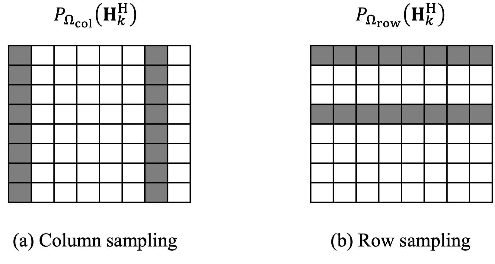
Figure 1: The description of the partially sampled entries of a cascaded channel, where the colored entries indicate the observed samples.

IV-A1 Column Sampling

For the subframes $b\in[N_{c}\times(M/N_{\rm RF})]$, the reflection vectors ${\bf v}_{b}$ and the RF combining matrices are constructed such that the columns whose indices are belong to ${\cal I}_{\rm col}$ are sampled. Towards this, these subframes are partitioned into $M/N_{\rm RF}$ blocks each having $N_{c}$ subframes. For each block $\ell\in[M/N_{\rm RF}]$, the reflection vectors are constructed as

$$\begin{bmatrix}{\bf v}_{1+(\ell-1)N_{c}}&\cdots&{\bf v}_{\ell N_{c}}\end{bmatrix}={\bf V}_{{\rm col}},$$ (7)

where ${\bf V}_{\rm col}$ is a $L\times N_{c}$ full-rank matrix. Namely, the reflection vectors are unchanged across the blocks. For the $\ell$-th block (i.e., $b=1+(\ell-1)N_{c},...,\ell N_{c}$), the RF combining matrices are constructed as

$${\bf C}_{b}={\bf C}_{[{\rm col},\ell]},$$ (8)

where ${\bf C}_{[{\rm col},\ell]}\in\mbox{\bb C}^{N_{\rm RF}\times M}$ is designed ${\bf C}_{[{\rm col},\ell]}^{{\sf H}}{\bf C}_{[{\rm col},\ell]}$ is the diagonal matrix having the $N_{\rm RF}$ numbers of 1’s at the locations $\{1+(\ell-1)N_{\rm RF},...,\ell N_{\rm RF}\}$. With these constructions, the received training signals in the $\ell$-th block are given by

$${\bf Z}_{[\ell,k]}^{\rm col} =\begin{bmatrix}{\bf z}_{[1+(\ell-1)N_{c},k]}&\cdots&{\bf z}_{[\ell N_{c},k]}\end{bmatrix}$$

$$={\bf C}_{[{\rm col},\ell]}{\bf H}_{k}^{{\sf H}}{\bf V}_{\rm col}+\tilde{{\bf N}}_{[\ell,k]}^{\rm col},$$

where $\tilde{{\bf N}}_{[\ell,k]}^{\rm col}=\begin{bmatrix}\tilde{{\bf n}}_{[1+(\ell-1)N_{c},k]}&\cdots&\tilde{{\bf n}}_{[\ell N_{c},k]}\end{bmatrix}$. From this, we can obtain

$${\bf C}_{[{\rm col},\ell]}^{{\sf H}}{\bf Z}_{[\ell,k]}^{\rm col}$$

$$=P_{\Omega_{[{\rm col},\ell]}}({\bf H}_{k}^{{\sf H}}){\bf V}_{\rm col}+P_{\Omega_{[{\rm col},\ell]}}({\bf C}_{[{\rm col},\ell]}^{{\sf H}}\tilde{{\bf N}}_{[\ell,k]}^{\rm col}),$$ (9)

where

$$\Omega_{[{\rm col},\ell]}=\{(1+(\ell-1)N_{\rm RF},j),...,(\ell N_{\rm RF},j):j\in{\cal I}_{\rm col}\}.$$

In order to estimate ${\bf S}_{\rm col}$, we use the training observations $\{{\bf M}_{[{\rm col},k]}:k\in[K]\}$, given by

$${\bf M}_{[{\rm col},k]} =\sum_{\ell=1}^{\frac{M}{N_{\rm RF}}}{\bf C}_{[{\rm col},\ell]}^{{\sf H}}{\bf Z}_{[\ell,k]}^{\rm col}$$

$$=P_{\Omega_{\rm col}}({\bf H}_{k}^{{\sf H}}){\bf V}_{\rm col}+\tilde{{\bf N}}_{[{\rm col},k]},$$ (10)

where $\Omega_{\rm col}=\bigcup_{\ell=1}^{\frac{M}{N_{\rm RF}}}\Omega_{[{\rm col},\ell]}$ and

$$\tilde{{\bf N}}_{[{\rm col},k]}=\sum_{\ell=1}^{\frac{M}{N_{\rm RF}}}P_{\Omega_{[{\rm col},\ell]}}({\bf C}_{[{\rm col},\ell]}^{{\sf H}}\tilde{{\bf N}}_{[\ell,k]}^{\rm col}).$$

Note that since ${\bf V}_{\rm col}$ is a full-rank, $P_{\Omega_{\rm col}}({\bf H}_{k}^{{\sf H}}){\bf V}_{\rm col}$ has the same column space with $P_{\Omega_{\rm col}}({\bf H}_{k}^{{\sf H}})$.

IV-A2 Row Sampling

During the remaining subframes (i.e., $b=N_{0}+1,...,N_{0}+L(N_{r}/N_{\rm RF})$), the row sampling is performed, i.e., the rows whose indices are belong to ${\cal I}_{\rm row}$ are sampled. Towards this, the subframes are partitioned into $N_{r}/N_{\rm RF}$ blocks each having $L$ subframes. For each block $\ell\in[N_{r}/N_{\rm RF}]$, the reflection vectors are constructed as

$$\begin{bmatrix}{\bf v}_{n_{0}+1+(\ell-1)L}&\cdots&{\bf v}_{n_{0}+\ell L}\end{bmatrix}={\bf V}_{{\rm row}},$$ (11)

where ${\bf V}_{{\rm row}}$ is a $L\times L$ unitary matrix. Namely, the reflection vectors are unchanged across the blocks. In the $\ell$-th block (i.e., $b=n_{0}+1+(\ell-1)L,...,n_{0}+\ell L$), the RF combining matrices are constructed as

$${\bf C}_{b}={\bf C}_{[{\rm row},\ell]},$$ (12)

where ${\bf C}_{[{\rm row},\ell]}$ is designed such that ${\bf C}_{[{\rm row},\ell]}^{{\sf H}}{\bf C}_{[{\rm row},\ell]}$ is the diagonal matrix having the $N_{\rm RF}$ numbers of 1’s at the locations $\{i_{1+(\ell-1)N_{\rm RF}},...,i_{\ell N_{\rm RF}}\}$. With these constructions, the received training signals in the $\ell$-th block are given by

$${\bf Z}_{[\ell,k]}^{\rm row} \stackrel{{\scriptstyle\Delta}}{{=}}\begin{bmatrix}{\bf z}_{[n_{0}+1+(\ell-1)L,k]}&\cdots&{\bf z}_{[n_{0}+\ell L,k]}\end{bmatrix}$$

$$={\bf C}_{[{\rm row},\ell]}{\bf H}_{k}^{{\sf H}}{\bf V}_{\rm row}+\tilde{{\bf N}}_{[\ell,k]}^{\rm row},$$ (13)

where $\tilde{{\bf N}}_{[\ell,k]}^{\rm row}\stackrel{{\scriptstyle\Delta}}{{=}}\begin{bmatrix}\tilde{{\bf n}}_{[n_{0}+1+(\ell-1)L,k]}&\cdots&\tilde{{\bf n}}_{[n_{0}+\ell L,k]}\end{bmatrix}$. From this, we can obtain

$${\bf C}_{[{\rm row},\ell]}^{{\sf H}}{\bf Z}_{[\ell,k]}^{\rm row}{\bf V}_{\rm row}^{{\sf H}}$$

$$=P_{\Omega_{[{\rm row},\ell]}}({\bf H}_{k}^{{\sf H}})+P_{\Omega_{[{\rm row},\ell]}}({\bf C}_{[{\rm row},\ell]}^{{\sf H}}\tilde{{\bf N}}_{[\ell,k]}^{\rm row}{\bf V}_{\rm row}^{{\sf H}}),$$ (14)

where $\Omega_{[{\rm row},\ell]}=\{(i_{(\ell-1)N_{\rm RF}+1},j),...,(i_{\ell N_{\rm RF}},j):j\in[L]\}$. In order to estimate $\{{\bf T}_{k}:k\in[K]\}$, we use the training observations $\{{\bf M}_{[{\rm row},k]}:k\in[K]\}$, given by

$${\bf M}_{[{\rm row},k]} =\sum_{\ell=1}^{\frac{N_{r}}{N_{\rm RF}}}{\bf C}_{[{\rm row},\ell]}^{{\sf H}}{\bf Z}_{[\ell,k]}^{\rm row}{\bf V}_{\rm row}^{{\sf H}}$$

$$=P_{\Omega_{{\rm row}}}({\bf H}_{k}^{{\sf H}})+\tilde{{\bf N}}_{[{\rm row},k]},$$ (15)

where $\Omega_{\rm row}=\bigcup_{\ell=1}^{\frac{N_{r}}{N_{\rm RF}}}\Omega_{[{\rm row},\ell]}$ and for $k\in[K]$,

$$\tilde{{\bf N}}_{[{\rm row},k]}=\sum_{\ell=1}^{\frac{N_{r}}{N_{\rm RF}}}P_{\Omega_{[{\rm row},\ell]}}\left({\bf C}_{[{\rm row},\ell]}^{{\sf H}}\tilde{{\bf N}}_{[\ell,k]}^{\rm row}{\bf V}_{\rm row}^{{\sf H}}\right).$$

IV-B Channel Estimation Method

We propose a collaborative low-rank approximation (CLRA)-based channel estimation method on the basis of the factorization of the cascaded channels in (6). The proposed method consists of the following steps:

• Using the column-sampled observations $\{{\bf M}_{[{\rm col},k]}:k\in[K]\}$ in (10), the dimension of the common column space (i.e., $N_{f}$) is estimated.

• Then, the $N_{f}$-dimensional common column space of $\{{\bf H}_{k}^{{\sf H}},\forall k\in[K]\}$ is estimated via CLRA. Namely, ${\bf S}_{\rm col}$ in (6) is estimated.

• Using the row-sampled observations ${\bf M}_{[{\rm row},k]}$ in (15), the user-specific coefficient matrices $\{{\bf T}_{k}:k\in[K]\}$ are jointly optimized using the special property of the cascaded channels.

The detailed procedures are provided below.

IV-B1 Estimation of the common column space

To estimate the ${\bf S}_{\rm col}$, we employ the training observations ${\bf M}_{[{\rm col},k]}(:,{\cal I}_{\rm col})$:

$${\bf M}_{[{\rm col},k]}(:,{\cal I}_{\rm col})={\bf H}_{k}(:,{\cal I}_{\rm col})^{{\sf H}}{\bf V}_{\rm col}+\tilde{{\bf N}}_{[{\rm col},k]}(:,{\cal I}_{\rm col}).$$

Note that since ${\bf V}_{\rm col}$ is a full-rank, ${\bf H}_{k}(:,{\cal I}_{\rm col})^{{\sf H}}{\bf V}_{\rm col}$ has the same column space with ${\bf H}_{k}(:,{\cal I}_{\rm col})^{{\sf H}}$. Define the $M\times M$ covariance matrix of the observations by

$${\bf K}_{\rm col}\stackrel{{\scriptstyle\Delta}}{{=}}\frac{1}{K}\sum_{k=1}^{K}{\bf M}_{[{\rm col},k]}(:,{\cal I}_{\rm col}){\bf M}_{[{\rm col},k]}(:,{\cal I}_{\rm col})^{{\sf H}}.$$ (16)

Also, the eigenvalue decomposition of ${\bf K}_{\rm col}$ is derived as

$${\bf K}_{\rm col}=\tilde{{\bf S}}_{\rm col}\hbox{\boldmath$\Sigma$}_{\rm col}\tilde{{\bf S}}_{\rm col}^{{\sf H}},$$ (17)

where $\tilde{{\bf S}}_{\rm col}$ is the eigenvectors corresponding to the eigenvalue matrix $\hbox{\boldmath$\Sigma$}_{\rm col}=\mbox{diag}([\lambda_{[{\rm col},1]},\lambda_{[{\rm col},2]},...,\lambda_{[{\rm col},M]}])$ and the eigenvalues $\lambda_{[{\rm col},\ell]}$’s are ordered in a descending order in magnitude. As suggested in [4], the $N_{f}$ can be efficiently estimated using the minimum description length (MDL) criterion [12] as

$$\hat{N}_{f} =\operatorname*{arg\,min}_{n}\left\{-\log\left(\frac{\prod_{i=n+1}^{M}\lambda_{[{\rm col},i]}^{\frac{1}{M-n}}}{\frac{1}{M-n}\sum_{i=n+1}^{M}\lambda_{[{\rm col},i]}}\right)^{(M-n)BT}\right.$$

$$\;\;\;\;\;\;\;\;\;\;\;\;\;\;\;\;\;\;\;\;\;\;\;\;\;\;\;\;\;\;\;\;\left.+\frac{1}{2}n(2M-n)\log(BT)\right\}.$$ (18)

This optimization is easily solved via the simple integer search over $n\in\mbox{\bb Z}^{+}$. As long as independent columns are sufficiently sampled (i.e., $|{\cal I}_{\rm col}|$ is large enough), the optimization below can yield a good $\hat{N}_{f}$-dimensional common column space [13]:

$${\bf S}_{\rm col}=\operatorname*{arg\,min}_{{\bf S}\in\mbox{\bb C}^{M\times\hat{N}_{f}},{\bf S}^{{\sf H}}{\bf S}={\bf I}}\left\|\left({\bf I}-{\bf S}{\bf S}^{{\sf H}}\right){\bf K}_{\rm col}\right\|_{2}^{2}.$$ (19)

From Eckart–Young–Mirsky Theorem [14], the optimal solution to the above problem is derived as

$$\hat{{\bf S}}_{\rm col}=\tilde{{\bf S}}_{\rm col}(:,[\hat{N}_{f}]).$$ (20)

IV-B2 Joint optimization of the coefficient matrices

Using the row-sampled observations $\{{\bf M}_{[{\rm row},k]}:k\in[K]\}$ and the estimated $\hat{{\bf S}}_{\rm col}$, the coefficient matrices $\{{\bf T}_{k}:k\in[K]\}$ are jointly optimized. From (1), we can identify the special property of the cascaded channels as follows:

$${\bf H}_{k}={\bf D}_{k}{\bf H}_{1},$$ (21)

where ${\bf D}_{k}\stackrel{{\scriptstyle\Delta}}{{=}}\mbox{diag}({\bf h}_{[r,k]})\mbox{diag}({\bf h}_{[r,1]})^{-1}$ is the $L\times L$ diagonal matrix. This is because

$${\bf H}_{k} =\mbox{diag}({\bf h}_{[r,k]}){\bf F}$$

$$=\mbox{diag}({\bf h}_{[r,k]})\left[\mbox{diag}({\bf h}_{[r,1]})^{-1}\mbox{diag}({\bf h}_{[r,1]})\right]{\bf F}$$

$$={\bf D}_{k}\mbox{diag}({\bf h}_{[r,1]}){\bf F}={\bf D}_{k}{\bf H}_{1}.$$ (22)

For ease of exposition, we let

$$\hat{{\bf T}}_{k}^{\rm LS}\stackrel{{\scriptstyle\Delta}}{{=}}\hat{{\bf S}}_{\rm col}({\cal I}_{\rm row},:)^{{\dagger}}{\bf M}_{[{\rm row},k]}({\cal I}_{\rm row},:),$$ (23)

which is in fact the solution of the individual least-square (LS) estimation. Leveraging this, we can jointly optimize the coefficient matrices by taking the solution of

$$\operatorname*{arg\,min}_{{\bf T}_{1},{\bf D}_{2},...,{\bf D}_{K}} \;\;\sum_{k=1}^{K}\left\|\hat{{\bf T}}_{k}^{\rm LS}-{\bf T}_{1}\left({\bf D}_{k}\right)^{{\sf H}}\right\|_{F}^{2}$$

subject to $$\;\;\;\;{\bf D}_{k}^{\prime}s\;\mbox{are diagonal matrices}.$$ (24)

We efficiently address the optimization problem in (24) via alternating optimization.

Initialization. From ${\bf D}_{k}=\mbox{diag}({\bf h}_{[r,k]})\mbox{diag}({\bf h}_{[r,1]})^{-1}$ in (21), we can see that for each $\ell\in[L]$,

$$\frac{h_{[r,k,\ell]}}{h_{[r,1,\ell]}}=\frac{{\bf H}_{k}(\ell,m)}{{\bf H}_{1}(\ell,m)}=\cdots=\frac{{\bf H}_{k}(\ell,M)}{{\bf H}_{1}(\ell,M)}.$$ (25)

Leveraging the (25) and the LS estimated channels $\hat{{\bf H}}_{k}=\hat{{\bf T}}_{k}^{\rm LS}{\bf S}_{\rm col}^{{\sf H}}$, the initial values $\hat{{\bf D}}_{k}^{(0)}$’s are determined such as

$$\hat{{\bf D}}_{k}^{(0)}=\mbox{diag}\left([\hat{d}_{[k,1]},...,\hat{d}_{[k,L]}]\right),$$ (26)

where

$$\hat{d}_{[k,\ell]}=\frac{1}{M}\sum_{m=1}^{M}\frac{\hat{{\bf H}}_{k}(\ell,m)}{\hat{{\bf H}}_{1}(\ell,m)},\;\ell\in[L].$$ (27)

Iterations. At the $t$-th iteration, the proposed alternating optimization is performed as follows:

• For the fixed $\hat{{\bf D}}_{k}^{(t-1)}$, our optimization can be formulated as a standard LS problem:

  $$\operatorname*{arg\,min}_{{\bf T}_{1}}\sum_{k=1}^{K}\left\|\hat{{\bf T}}_{k}^{\rm LS}-{\bf T}_{1}\left(\hat{{\bf D}}_{k}^{(t-1)}\right)^{{\sf H}}\right\|_{F}^{2},$$ (28)

  where $\hat{{\bf D}}_{1}^{(t-1)}={\bf I}$ during iterations. The optimal solution is derived as

  $$\hat{{\bf T}}_{1}^{(t)}=\left(\sum_{k=1}^{K}\hat{{\bf T}}_{k}^{\rm LS}\hat{{\bf D}}_{k}^{(t-1)}\right)\left(\sum_{k=1}^{K}\left(\hat{{\bf D}}_{k}^{(t-1)}\right)^{{\sf H}}\hat{{\bf D}}_{k}^{(t-1)}\right)^{-1}.$$ (29)

• For the fixed $\hat{{\bf T}}_{1}^{(t)}$, our optimization can be formulated as

  $$\operatorname*{arg\,min}_{{\bf D}_{k}}\left\|\hat{{\bf T}}_{k}^{\rm LS}-{\bf T}_{1}^{(t)}\left({\bf D}_{k}\right)^{{\sf H}}\right\|_{F}^{2},$$ (30)

  for $k\in[K]$. This LS problem is easily solved as

  $$\hat{{\bf D}}_{k}^{(t)}={\rm diag}\left({\bf R}(:,{\cal I}_{L})^{\dagger}\hat{{\bf t}}_{k}^{\rm LS}({\cal I}_{L})\right),$$ (31)

  where ${\bf R}={\bf I}\otimes\hat{{\bf T}}_{1}^{(t)}\in\mbox{\bb C}^{N_{f}L\times L^{2}}$, $\hat{{\bf t}}_{k}^{\rm LS}={\rm vec}(\hat{{\bf T}}_{k}^{\rm LS})\in\mbox{\bb C}^{L^{2}\times 1}$ is the vectorization of $\hat{{\bf T}}_{k}^{\rm LS}$, and ${\cal I}_{L}=\{\ell+(\ell-1)L:\ell\in[L]\}$.

After $t_{\rm max}$ iterations, the estimated cascaded channels are given by

$$\hat{{\bf H}}_{k}=\hat{{\bf D}}_{k}^{(t_{\rm max})}\left(\hat{{\bf T}}_{1}^{(t_{\rm max})}\right)^{{\sf H}}\hat{{\bf S}}_{\rm col}^{{\sf H}},\;k\in[K].$$ (32)

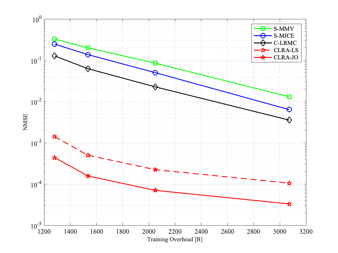
Figure 2: Average NMSE versus training overhead, where ${\sf SNR}=20$dB, $N_{h_{k}}=8,\forall k\in[K]$, and $M_{f}=4$.

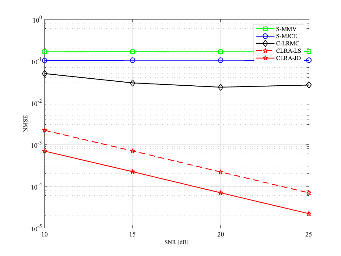
Figure 3: Average NMSE versus SNR, where $B=2048$, $N_{h_{k}}=8,\forall k\in[K]$, and $N_{f}=4$.

V Simulation Results

We consider the RIS-aided MU-MIMO system with $M=128$, $L=128$, $N_{\rm RF}=4$, and $K=10$. For training, each user transmits an orthogonal pilot sequence of the length $T=10$ and the power $P_{k}=P$ for $k\in[K]$. Hence, all $K$ users explore the same signal-to-noise ratio (SNR), defined as ${\sf SNR}=10\log(P/\sigma^{2})\mbox{[dB]}$, where $\sigma$ is given in (4). Regarding wireless channels, the power is equally divided into each signal path, the phase of a channel gain is chosen uniformly and randomly from $[0,\pi]$, and the angle of all AoDs and AoAs are chosen uniformly and randomly from $[0,\pi]$. Following the performance metric in the related works [3, 4, 7, 8], we use the normalized mean square error (NMSE), given by

$$\mbox{NMSE}=\mbox{\bb E}\left[\frac{1}{K}\sum_{k=1}^{K}\frac{\|\hat{{\bf H}}_{k}-{\bf H}_{k}\|_{F}^{2}}{\|{\bf H}_{k}\|_{F}^{2}}\right].$$ (33)

The expectation is evaluated by Monte Carlo simulations with $100$ trials. We compare the NMSE performances of the proposed method (named CLRA-JO) with the state-of-the-art CS-based S-MMV [3] and S-MJCE [4], and the LRMC-based C-LRMC [8]. In the proposed method, when the coefficient matrices can be obtained from the LS estimation ((i.e., $\hat{{\bf T}}_{k}^{\rm LS}$ in (23)) instead of the joint optimization, this simplified method is named CLRA-LS. This method is considered to identify the performance gain of the joint optimization in Section IV-B2. The CS-based methods use the hyperparameters as $r=256$ and $\lambda=10^{-4}$, where $r$ denotes the resolution to form a dictionary matrix and $\lambda>0$ denotes a regularization parameter. Note that $r$ can control the tradeoff between the estimation accuracy and the computational complexity [4]. All of the aforementioned methods require the iterations with $I_{\rm C}=10^{2}$, $I_{\rm L}=10^{3}$, $I_{\rm in}=5\times 10^{2}$, $I_{\rm out}=10^{4}$, where $I_{\rm C}$ denotes the number of iterations for CLRA-JO, $I_{\rm L}$ denotes the number of iterations for C-LRMC, and $I_{\rm in}$ and $I_{\rm out}$ denote the number of iterations for inner- and outer-loop of S-MJCE, respectively. These values are optimized via experiments.

We provide the computational complexities of the proposed and benchmark methods. To characterize the complexities, we count the number of complex multiplication (CM) as in [4]. For estimating a common column space, the eigenvalue decomposition is performed, which requires the following computational complexity:

$$\Psi_{\mbox{\scriptsize CCS}}=\mathcal{O}(M^{3}).$$ (34)

This estimation is used for all methods. Then, the computational complexities of C-LRMC, S-MMV, S-MJCE, and the proposed CLRA are respectively computed as

$$\Psi_{\mbox{\scriptsize C-LRMC}} =\Psi_{\mbox{\scriptsize CCS}}+\mathcal{O}(I_{\rm L}MLN_{f})$$

$$\Psi_{\mbox{\scriptsize S-MMV}} =\Psi_{\mbox{\scriptsize CCS}}+\mathcal{O}(r^{2}MB)$$

$$\Psi_{\mbox{\scriptsize S-MJCE}} =\Psi_{\mbox{\scriptsize CCS}}+\Psi_{\mbox{\scriptsize S-MMV}}+\mathcal{O}(I_{\rm out}I_{\rm in}r^{3}L^{3})$$

$$\Psi_{\mbox{\scriptsize CLRA-JO}} =\Psi_{\mbox{\scriptsize CCS}}+\mathcal{O}(I_{\rm C}L^{3}),$$

where the second terms of $\Psi_{\mbox{\scriptsize C-LRMC}}$ and $\Psi_{\mbox{\scriptsize S-MMV}}$ are from matrix multiplications during iterations, the second terms of $\Psi_{\mbox{\scriptsize CLRA-JO}}$ and the third term of $\Psi_{\mbox{\scriptsize S-MJCE}}$ originated from matrix inversions during loop.

Fig. 2 shows the NMSE performances of the proposed and benchmark methods as a function of training overhead $B$. Note that compared with the performances when full-digital architectures are adopted [3, 4, 6], the required training overheads in Fig. 2 and Fig. 3 are $M/N_{\rm RF}=32$ times larger due to the use of hybrid receiver architectures. The proposed CLRA-JO can significantly outperform the benchmark methods for all training overheads. To achieve the $\mbox{NMSE}=10^{-4}$, CLRA-JO requires the training overhead $B=1800$, whereas the benchmark methods cannot achieve it even with larger training overheads. In comparisons with CLRA-LS, we can see that the proposed joint optimization to use the special property of cascaded channels indeed improves the estimation accuracy of user-specific coefficient matrices. Fig. 3 shows the NMSE performances of the proposed and benchmark methods as a function of SNR. Compared with the benchmark methods, the proposed CLRA-JO can attain much higher performance gains as SNR increases. We emphasize that the accuracy of the CS-based methods stop improving, even if SNR increases. This is due to the well-known grid-mismatch problem [7, 8]. We remark that C-LRMC, CLRA-LS, and CLRA-JO, based on hybrid receiver architectures, have much lower computational complexities than the CS-based methods. Compared with S-MMV (i.e., the CS method having the lowest complexity), they only cost $0.39\%$, $0.025\%$, and $1.23\%$ complexities, respectively. Our simulation results indeed demonstrate the superiority of our algorithm, especially when a hybrid receiver architecture is used for RIS-aided mmWave MU-MIMO systems.

VI Conclusion

We investigated the channel estimation problem for RIS-aided mmWave MU-MIMO systems, in particular when hybrid receiver architectures are adopted. In this system, we proposed the simple yet efficient channel estimation method (named CLRA-JO), in which the common column space is estimated via collaborative low-rank approximation (CLRA) and the user-specific coefficient matrices are jointly optimized using the special structure of the cascaded channels. Via simulations, it is demonstrated that the proposed CLRA-JO can yield better estimation accuracy than the state-of-the-art methods while having lower training overhead. Our on-going work is to conduct a theoretical analysis of the proposed method.

References

• [1] R. Long, Y.-C. Liang, Y. Pei, and E. G. Larsson, “Active intelligent reflecting surface for simo communications,” in IEEE Global Communications Conference.   IEEE, 2020, pp. 1–6.
• [2] H. Wymeersch, J. He, B. Denis, A. Clemente, and M. Juntti, “Radio localization and mapping with reconfigurable intelligent surfaces: Challenges, opportunities, and research directions,” IEEE Vehicular Technology Magazine, vol. 15, no. 4, pp. 52–61, 2020.
• [3] C.-R. Tsai, Y.-H. Liu, and A.-Y. Wu, “Efficient compressive channel estimation for millimeter-wave large-scale antenna systems,” IEEE Transactions on Signal Processing, vol. 66, no. 9, pp. 2414–2428, 2018.
• [4] J. Chen, Y.-C. Liang, H. V. Cheng, and W. Yu, “Channel estimation for reconfigurable intelligent surface aided multi-user mmwave mimo systems,” IEEE Transactions on Wireless Communications, 2023.
• [5] Y. Chi, L. L. Scharf, A. Pezeshki, and A. R. Calderbank, “Sensitivity to basis mismatch in compressed sensing,” IEEE Transactions on Signal Processing, vol. 59, no. 5, pp. 2182–2195, 2011.
• [6] R. Schroeder, J. He, and M. Juntti, “Channel estimation for hybrid ris aided mimo communications via atomic norm minimization,” in 2022 IEEE International Conference on Communications Workshops (ICC Workshops).   IEEE, 2022, pp. 1219–1224.
• [7] H. Chung and S. Kim, “Efficient two-stage beam training and channel estimation for ris-aided mmwave systems via fast alternating least squares,” in ICASSP 2022-2022 IEEE International Conference on Acoustics, Speech and Signal Processing (ICASSP).   IEEE, 2022, pp. 5188–5192.
• [8] J. Lee and S. Hong, “Channel estimation for ris-aided mmwave mu-mimo systems: Collaborative low-rank matrix completion approach,” in IEEE International conference on Network Intelligence and Digital Content (IC-NIDC).   IEEE, 2024, pp. 1–5.
• [9] I. Ahmed, H. Khammari, A. Shahid, A. Musa, K. S. Kim, E. De Poorter, and I. Moerman, “A survey on hybrid beamforming techniques in 5g: Architecture and system model perspectives,” IEEE Communications Surveys & Tutorials, vol. 20, no. 4, pp. 3060–3097, 2018.
• [10] A. F. Molisch, V. V. Ratnam, S. Han, Z. Li, S. L. H. Nguyen, L. Li, and K. Haneda, “Hybrid beamforming for massive mimo: A survey,” IEEE Communications magazine, vol. 55, no. 9, pp. 134–141, 2017.
• [11] H. Liu, X. Yuan, and Y.-J. A. Zhang, “Matrix-calibration-based cascaded channel estimation for reconfigurable intelligent surface assisted multiuser mimo,” IEEE Journal on Selected Areas in Communications, vol. 38, no. 11, pp. 2621–2636, 2020.
• [12] M. Wax and T. Kailath, “Detection of signals by information theoretic criteria,” IEEE Transactions on acoustics, speech, and signal processing, vol. 33, no. 2, pp. 387–392, 1985.
• [13] J. Chae, P. Narayanamurthy, S. Bac, S. M. Sharada, and U. Mitra, “Column-based matrix approximation with quasi-polynomial structure,” in ICASSP 2023-2023 IEEE International Conference on Acoustics, Speech and Signal Processing (ICASSP).   IEEE, 2023, pp. 1–5.
• [14] C. Eckart and G. Young, “The approximation of one matrix by another of lower rank,” Psychometrika, vol. 1, no. 3, pp. 211–218, 1936.