Quantifying energy landscape of oscillatory systems: Explosion, pre-solution, and diffusion decomposition

Abstract

The energy landscape theory finds its both extensive and intensive application in studying stochastic dynamics of physical and biological systems. Although the weighted summation of the Gaussian approximation (WSGA) approach has been proposed for quantifying the energy landscape in multistable systems by solving the diffusion equation approximately from moment equations, we are still lacking an accurate approach for quantifying the energy landscape of the periodic oscillatory systems. To address this challenge, we propose an approach, called the diffusion decomposition of the Gaussian approximation (DDGA). Using typical oscillatory systems as examples, we demonstrate the efficacy of the proposed DDGA in quantifying the energy landscape of oscillatory systems and corresponding stochastic dynamics, in comparison with existing approaches. By further applying the DDGA to a high-dimensional cell cycle network, we are able to uncover more intricate biological mechanisms in cell cycle, which cannot be discerned using previously developed approaches.

I Introduction

Biophysical systems are usually governed by complex networks. Representative systems include the dynamics induced by gene regulatory networks [1, 2, 3], neuronal networks [4, 5, 6], and human mobility networks [7, 8]. A traditional way to study these dynamics is through deterministic mathematical modeling [1, 2]. However, stochasticity, an omnipresent phenomenon, often plays critical roles in influencing the dynamical behaviors of real-world systems [9, 10, 11]. Correspondingly, the energy landscape approach has been developed, becoming one of the mainstream ways to study the stochastic dynamics of biophysical systems [12, 13, 14, 15, 3, 16, 17, 18, 19]. For example, some approaches have been developed to construct the energy landscape for high-dimensional gene regulatory networks [3, 20], by approximately solving the Fokker-Planck equation (FPE) [21].

Although the framework above seems to be feasible, nonlinear driving forces and high-dimensional systems often pose challenges in solving the FPE, even approximately. To address this, the weighted summation of Gaussian approximation (WSGA) approach has been proposed [3, 22], which leverages the Gaussian distributions with appropriate weight vectors/functions to approximate probability density functions by solving moment equations. Variants of this approach rooted in the WSGA have been extensively employed in diverse biophysical systems [23, 20, 24, 22]. However, the WSGA owns certain limitations, including its confinement within the skewness constraints of the Gaussian distribution itself and its limited efficacy in application to the periodic oscillatory systems. For the first limitation, an enhanced approach called the extended Gaussian approximation (EGA), has been proposed to incorporate the high order moments information for capturing the asymmetry of the intricate systems [22], while, for the second, challenges remain.

In fact, oscillatory dynamics bring substantial difficulties to typical approaches, particularly in handling the moment equations of the WSGA. For instance, introducing oscillation into the WSGA’s covariance equations frequently results in an “explosion” solution that diverges towards infinity, rendering the original WSGA ineffective. Fortunately, before being puzzled by this counterintuitive phenomenon, researchers have already adopted a simpler substitute for the WSGA, termed the Mean-Field Approximation (MFA) [3, 25, 26]. The MFA omits correlations to ensure self-consistency of each variable, thereby simplifying the covariance matrix into a diagonal form. Consequently, the MFA significantly reduces computational complexity and coincidentally addresses the covariance explosion issue. Thus, the invalidation of the WSGA’s applicability has not been formally investigated particularly to oscillatory systems. While the MFA’s simplification enhances some convenience, there remains a need to reintegrate the correlation information when necessary. Kang et al. introduced an approach to compute complete covariance matrices for multistable systems having steady states, thereby extending the accuracy of the MFA [20]. However, the theoretical underpinnings of analogous techniques for oscillatory systems and explanations for the “covariance explosion” remain absent, requiring urgent attention and exploration.

In this article, we present a feasible approximation approach, named as diffusion decomposition of the Gaussian approximation (DDGA), for quantifying the landscape of periodic oscillatory systems characterized by a limit cycle. We apply the DDGA to diverse gene regulatory networks with various dimensions. Additionally, we delve into the mathematical understanding of the “covariance explosion” phenomenon and provide theoretical underpinnings for the WSGA-based approaches. Specifically, our approach encompasses several key steps. First, we provide a pre-solution which is a distribution on the limit cycle, a low-dimensional stable manifold. This facilitates the description of the low-dimensional dynamics and a comprehensive assessment of the oscillatory structure. We obtain this pre-solution by solving the FPE constrained to the limit cycle, markedly enhancing the precision of the weight function in the WSGA. Subsequently, we incorporate diffusion effects within the framework of the WSGA. We demonstrate that the diffusion process on the orthogonal normal plane of the limit cycle can be approximated as a stationary process, thereby simplifying the majority of the ordinary differential equations (ODEs) into matrix equations. Consequently, the computation cost for the covariance matrix is extremely reduced. The DDGA dissects the stochastic evolution into the tangential and the other $(n-1)$-dimensional orthogonal directions, effectively overcoming the contradiction between the necessity for the omission of non-diagonal covariance and “covariance explosion”.

To illustrate the advantages of the DDGA, we apply it to three distinct but representative oscillatory systems of dimensions 2, 6, and 44, respectively. Through using two probability measure indices and time-cost analysis, we compare the DDGA against two established methods, the WSGA and the EGA. The findings reveal that our approach offers improved precision and higher efficiency in quantifying the landscape of oscillatory systems. Of note, the DDGA yields higher accurate biological predictions, exemplified by the identification of the landscape explosion phenomenon in a 6-dimensional synthetic oscillatory network and the detection of new basins and checkpoints in a 44-dimensional mammalian cell cycle network. All these were not discernible using the original WSGA. These discoveries underscore the utility of the DDGA in effectively quantifying the landscape of oscillatory dynamics. To offer comprehensive insights into the predictions made by the DDGA, we employ flux and limit planes in synthetic oscillatory networks to elucidate the coexistence of the explosion phenomenon and the stability of the limit cycle.

II Results and Discussions

II.1 Weighted summation of Gaussian approximation

In this section, we first review the WSGA, an effective method of approximating the probability distribution of the stochastic systems from the moment equations and the weighted summation. In a stochastic dynamical system, the diffusion force provides the stochasticity, leading us to focus on the distribution rather than a single trajectory. The FPE is used to characterize this distribution [21, 27]. Under It$\hat{\text{o}}$’s interpretation, the distribution $\rho(\boldsymbol{x},t)$ is described by

$$\frac{\partial\rho(\boldsymbol{x},t)}{\partial t}= -\sum\limits_{i=1}^{n}\frac{\partial}{\partial x_{i}}\Big{[}F_{i}(\boldsymbol{x})\rho(\boldsymbol{x},t)\Big{]}$$ (1)

$$+ D\sum\limits_{i=1}^{n}\sum\limits_{j=1}^{n}\frac{\partial^{2}}{\partial x_{i}\partial x_{j}}\Big{[}d_{ij}(\boldsymbol{x})\rho(\boldsymbol{x},t)\Big{]},$$

where $\boldsymbol{F}=(F_{1},\dots,F_{n})$ represents the drift force, $\boldsymbol{d}=(d_{ij})_{1\leq i,j\leq n}$ represents the diffusion force, and $D$ is the diffusion coefficient. The FPE provides a precise description of stochastic differential equations, but it is hard to solve as $\boldsymbol{F}$ is nonlinear. Thus, it is necessary to give an approximation of the solution, such as the WSGA. In this approach, we use the Gaussian distribution to provide a local approximation, which is uniquely characterized by the first two moment equations [28, 22]:

$$\begin{cases}\begin{aligned} \dot{\boldsymbol{\mu}}(t)=&F(\boldsymbol{\mu}(t)),\end{aligned}\\ \begin{aligned} \dot{\boldsymbol{\Sigma}}(t)=&\boldsymbol{\Sigma}(t)\boldsymbol{A}^{\top}(t)+\boldsymbol{A}(t)\boldsymbol{\Sigma}(t)\\ +&D\Big{[}\boldsymbol{d}(\boldsymbol{\mu}(t))+\boldsymbol{d}^{\top}(\boldsymbol{\mu}(t))\Big{]},\end{aligned}\end{cases}$$ (2)

where the elements of the Jacobi matrix $\boldsymbol{A}(t)$ are specified as $\boldsymbol{A}_{(i,j)}(t)=\frac{\partial F_{i}(\boldsymbol{\mu}(t))}{\partial x_{j}(t)}$, $\boldsymbol{\mu}$ is the expectation vector, and $\boldsymbol{\Sigma}$ is the covariance matrix. For systems we often encounter in gene network systems, we need to work out how to characterize multiple stable states or limit cycles. As such, we demonstrate that the weighted summation provides a theoretical and efficient approach for approximating the multistable as well as oscillatory system[22]. Specifically, for the multistable systems, we describe a multistable distribution of the system with $N$ stable states $S_{i}\,(1\leq i\leq N)$ by

$$\rho(\boldsymbol{x},+\infty)=\sum\limits_{\begin{subarray}{c}i=1\\ \boldsymbol{\mu}(+\infty;\boldsymbol{u}_{i})=\mu_{i}\end{subarray}}^{N}\omega_{i}\times GA(+\infty;u_{i})(\boldsymbol{x}),$$

$$GA(t;u_{i})(\boldsymbol{x})=\frac{1}{\sqrt{(2\pi)^{n}\det(\boldsymbol{\Sigma}(t;u_{i}))}}\times$$

$$\exp\left[-\frac{1}{2}\Big{(}\boldsymbol{x}-\boldsymbol{\mu}(t;u_{i})\Big{)}^{\top}\boldsymbol{\Sigma}(t;u_{i})^{-1}\Big{(}\boldsymbol{x}-\boldsymbol{\mu}(t;u_{i})\Big{)}\right].$$

Here, $\omega_{i}$ is the corresponding weight for the $i$-th peak which is calculated by the deterministic ODEs, $\mu_{i}$ is the location of $S_{i}$ in $\mathbb{R}^{n}$, and $\boldsymbol{u}_{i}$ is any one of the representative elements which move towards $S_{i}$ [22]. Meanwhile, $GA(t;*)$ is known as the Gaussian approximation, the origin approach of the WSGA.

For the periodic oscillatory system, another type of dynamical system, we have proposed that the WSGA is suitable for approximating the steady state probability distribution by integral summation [3, 22]. That is, for its limit cycle with period $T$ and a continuous weight function $\omega(t)$ defined on $[0,T]$ with $\int_{0}^{T}\omega(t)\text{d}t=1$, we perform the WSGA as

$$\rho(\boldsymbol{x})=\int_{0}^{T}\omega(t)\times\mathcal{N}(\boldsymbol{\mu}(t),\boldsymbol{\Sigma}(t))(\boldsymbol{x})\text{d}t,$$

in which $\mathcal{N}(\boldsymbol{\mu}(t),\boldsymbol{\Sigma}(t))$ is the Gaussian distribution at time $t$ with mean $\boldsymbol{\mu}(t)$ and covariance matrix $\boldsymbol{\Sigma}(t)$. In the previous practice, we usually choose weight function $\omega(t)$ as a constant function, i.e., $\omega(t)\equiv\frac{1}{T}$, for$t\in[0,T]$. An integral with the weight function can be regarded as another weighted summation approach in the continuous situation.

Moreover, some extended moment approaches have been developed to approximate more detailed information of the system, such as the EGA, which considers the third moments to describe the skewness of the system, a missing property in the WSGA [22] (see Methods for a detailed description of the EGA).

Although the WSGA greatly reduces the calculation cost avoiding numerically, and directly solving the FPE, in those high-dimensional biological systems such as genetic circuits, it still highly costly to solve the covariance equations. Thus, the MFA approach was proposed to overcome the dimensional curse emergent in the numerical calculation. In the MFA, the high-dimensional probability $P(x_{1},x_{2},\dots,x_{n};t)$ is split into the product of $n$ individual one-dimensional probability: $P(x_{1},x_{2},\dots,x_{n};t)\sim\prod\limits_{i=1}^{n}P(x_{i},t)$ which can be solved self-consistently [29, 3]. The MFA directly ignores the covariance of the two different variables, which simplifies the covariance matrix $\boldsymbol{\Sigma}$ into a diagonal matrix. Therefore, it is worthwhile computing the non-diagonal element of the covariance matrix to describe the interaction between different variables. Kang et al. proposed an approach for calculating the whole covariance matrix in the multistable systems by considering the steady-state solution of those moments [20] (See details in Methods). While their approach improves the accuracy of approximation by solving the complete covariance matrix, they also change the covariance ODEs into the matrix multiplication, which thus greatly speeds up the computation. Of note, the form of the covariance equations itself does not guarantee the semidefinite positivity of the solution, which is an essential condition for the Gaussian distribution. In this work, we prove that the covariance matrix $\boldsymbol{\Sigma}$ in the Gaussian approximation is a semidefinitely positive matrix (see more details in Supplementary Material). It further complements the mathematical foundation for the application of the Gaussian approximation in the multistable systems.

II.2 Limit cycle leads to an explosion of the variance in moment equations

As we introduced above for the moment approaches, the second-moment equations $\dot{\boldsymbol{\Sigma}}(t)=\boldsymbol{\Sigma}(t)\boldsymbol{A}^{\top}(t)+\boldsymbol{A}(t)\boldsymbol{\Sigma}(t)+D\Big{[}\boldsymbol{d}(\boldsymbol{\mu}(t))+\boldsymbol{d}^{\top}(\boldsymbol{\mu}(t))\Big{]}$ play an important role in approximation. This rises from the fact that in the assumption of the WSGA [28], the first-moment equations describe the deterministic evolution which has been sufficiently studied in traditional mathematical modeling [1, 2, 13], while the covariance equations directly depict the “width” of a Gaussian peak, which significantly influences the landscape through the WSGA. Actually, Kang et al.’s approach maintains all of the non-diagonal elements of the covariance matrix, leading to a more accurate approximation than the MFA.

Although those approaches obtain great achievement in the multistable systems, they always fail to cope with another type of nonlinear complex systems, the periodic oscillatory systems, in which the landscape looks like a Mexican hat around the limit cycle [3]. In many periodic systems, we find that the covariance $\boldsymbol{\Sigma}$ oscillates and diverges to infinity as $t\rightarrow+\infty$. For instance, consider a paradigmatic noise-perturbed dynamical system with the unit cycle in $\mathbb{R}^{2}$: $x^{2}+y^{2}=1$ as its stable limit cycle:

$$\begin{cases}\begin{aligned} \dot{x}=-y+(1-x^{2}-y^{2})x+\Gamma_{1},\end{aligned}\\ \begin{aligned} \dot{y}=x+(1-x^{2}-y^{2})y+\Gamma_{2},\end{aligned}\\ x(0)=1,\,y(0)=0,\end{cases}$$ (3)

where $\Gamma_{1,2}$ represent the corresponding Gaussian white noises. Let $\boldsymbol{\Sigma}$ be the second moment with $d(x)=I_{2}$. Since the theoretical solution of $x,y$ can be calculated as $x(t)=\cos t,\,y(t)=\sin t$, to solve the covariance equation Eq. 2 with

$$\boldsymbol{A}=\begin{pmatrix}-2\cos^{2}t&-1-2\sin t\cos t\\ 1-\sin t\cos t&-2\sin^{2}t\end{pmatrix},$$

we perform an orthogonal transformation through the matrix

$$Q=\begin{pmatrix}\cos t&-\sin t\\ \sin t&\cos t\end{pmatrix}$$

and get the covariance after the orthogonal transformation $\hat{\boldsymbol{\Sigma}}=Q^{\top}\boldsymbol{\Sigma}Q$. Then we have (see more details in Supplementary Material)

$$\dot{\hat{\boldsymbol{\Sigma}}}(t)=\begin{pmatrix}-4\hat{\sigma}_{11}&-2\hat{\sigma}_{12}\\ -2\hat{\sigma}_{21}&0\end{pmatrix}+2DI_{2}.$$ (4)

Thus, the theoretical solution is obtained as

$$\begin{cases}\begin{aligned} \hat{\sigma}_{11}(t)=(\hat{\sigma}_{11}(0)-\frac{D}{2})\text{e}^{-4t}+\frac{D}{2}\longrightarrow\frac{D}{2}\quad(t\longrightarrow+\infty),\end{aligned}\\ \begin{aligned} \hat{\sigma}_{12}(t)=\hat{\sigma}_{12}(0)\text{e}^{-2t}\longrightarrow 0\quad(t\longrightarrow+\infty),\end{aligned}\\ \begin{aligned} \hat{\sigma}_{21}(t)=\hat{\sigma}_{21}(0)\text{e}^{-2t}\longrightarrow 0\quad(t\longrightarrow+\infty),\end{aligned}\\ \begin{aligned} \hat{\sigma}_{22}(t)=\hat{\sigma}_{22}(0)+2Dt\longrightarrow+\infty\quad(t\longrightarrow+\infty).\end{aligned}\end{cases}$$

The covariance $\boldsymbol{\Sigma}(t)$ oscillates and diverges to infinity for the direction along the limit cycle ($\hat{\sigma}_{22}\longrightarrow+\infty$). For the similar reasons, effective mathematical tools are lacking for studying the stochastic dynamics of the periodic oscillatory systems so far.

The example mentioned above reflects that the WSGA loses its efficacy in oscillatory systems. Consequently, We are concerned about the reason why the existent methods become ineffective. Approaches based on the WSGA calculate the covariance using the converged ODEs, while the convergence relies on a condition that the eigenvalues of the evolution matrix $\boldsymbol{A}\otimes I+I\otimes\boldsymbol{A}$ are all negative, due to the Lyapunov’s stability criterion (see more details in Methods). By a fact that $\boldsymbol{A}v=\lambda v$ implies

$$(\boldsymbol{A}\otimes I+I\otimes\boldsymbol{A})\text{vec}(vv^{\top})=2\lambda\cdot\text{vec}(vv^{\top})$$

for $\lambda<0$, the condition mentioned above further relies on its necessary condition that all the eigenvalues of $\boldsymbol{A}$ are negative, which meets the properties of the attractors. However, for the periodic oscillatory systems, the negative properties may fail along the tangential direction of the limit cycle. For instance, in Eq. 3, the eigenvalues of the evolution matrix in Eq. 4 are -4, -2, -2, and 0, where the direction of eigenvector corresponding to eigenvalue $0$, which is the tangential vector $(-\sin t,\cos t)$, leads to the divergence of iteration.

We further explore, in the WSGA-based approaches, the mathematical assumption that becomes ineffective in oscillatory systems and leads to an “explosion of the covariance”. We attribute the divergence of covariance to the fact that the approaches based on the WSGA only locally study the system from the $\Omega$-expansion [30] and thus are lack of global consideration. For a global stable structure such as the limit cycles, the divergence of covariance for the direction along the stable sub-manifold results in general diffusion inside this manifold, which implies that the local distribution eventually spreads out to the whole manifold. The inconsistency between the local analysis and the global dynamics in oscillatory systems brings obstacles to the WSGA-based approaches. Particularly, in Eq. 3, the covariance along the tangential direction, i.e. $\hat{\sigma}_{22}$, diverges to infinity, making the distribution spread out along the limit cycle.

Meanwhile, by omitting the relationship between the variables, the MFA provides an intuitive covariance matrix that oscillates periodically. It has overcome the problems of divergence to a certain extent, but still lacks a global consideration of the structure. Moreover, the MFA loses too much information and performs poorly in some oscillatory systems of lower dimensions. It seems that avoiding the covariance divergence requires abandoning a large amount of correlation information. Thus, it is urgent to further develop a WSGA-based approach, avoiding the problem of the covariance divergence in the limit cycle systems, while retaining as much the covariance and the other correlation information as possible. As such, it can greatly improve the accuracy in characterizing and approximating the stochastic periodic dynamics.

II.3 An efficient and accurate approximation of landscape in limit-cycle systems by pre-solution and diffusion

In periodic oscillatory systems, the solutions obtained from the covariance equations diverge, rendering the traditional WSGA ineffective. In this section, we propose an approximation approach that addresses the limitations of the original WSGA while retaining its simplicity and effectiveness. Importantly, our approach takes into account the influence of the limit cycle as a low-dimensional stable manifold on the landscape. Leveraging the geometric properties of the stable manifold and under a few reasonable assumptions, we demonstrate that most of the ODEs in WSGA can be approximated by the matrix equations. This significantly enhances the computational efficiency. In high-dimensional oscillatory systems, our approach is much faster than the other approaches used in the previous studies (see details in Table S1). Furthermore, through several numerical examples, we demonstrate the superior efficacy of our approach in comparison to the commonly-used approximation approaches in capturing the landscape of the periodic oscillatory systems. This provides a more accurate and efficient tool for investigating the dynamics of such biophysical systems and their periodic behaviors.

The original WSGA approach incorporates the idea of “local diffusion of individuals along noiseless trajectories”. While this approach has limitations in global exploration, it provides us with valuable insights. Following the same guiding principle, we approximate the landscape features on the stable manifold implied by the system and consider the diffusion process under the influence of noise to obtain a global approximation. In the following demonstration, we are to illustrate our approach using the limit cycle, a familiar one-dimensional stable manifold. Specifically, the system evolves according to the Langevin equation, which consists of a driving force and a diffusion noise. Without considering the noise, the driving force is tangential to the limit cycle (which represents the noiseless trajectory). By considering a homeomorphic mapping of the limit cycle onto the quotient space $[0,1]/\partial{[0,1]}$ (Here, the operator $\partial$ represents the topological boundary, i.e., $\partial[0,1]=\{0,1\}$), the evolution follows the one-dimensional Langevin dynamics. In other words, if the system evolves without noise, the process is entirely confined to this one-dimensional manifold. Consequently, there exist corresponding Fokker-Planck equations and explicit solutions on this one-dimensional manifold. This approach fully takes into account the global influence of the limit cycle as a stable manifold on the system evolution, rather than focusing solely on the local aspects like the original WSGA. Finally, we consider the impact of the diffusion term on the system.

To better illustrate the process of our method, we assume that the diffusion coefficients are homogeneous and constant, i.e., $\boldsymbol{d}(x)=I_{n}$. In other words, the diffusion strength is always a constant $D$. Moreover, we list the method for the general cases as Eq. 1 in the Supplementary Material. Under this assumption, we first consider the impact of the Langevin dynamics only on the limit cycle, a sub-manifold of the system. Since the driving force acts tangentially along the limit cycle, its effect is to induce periodic oscillation around the limit cycle. Therefore, restricting the driving force to the sub-manifold does not alter its behavior. As for the diffusion term $\boldsymbol{\Gamma}\sim N(0,I_{n})$ in the original stochastic process, which is induced by a small noise, we decompose it orthogonally into the noise along the unit tangential direction $v_{1}$ of the limit cycle and noise along the ($n-1$)-dimensional normal plane

$$\boldsymbol{\Gamma}=\boldsymbol{\Gamma}_{t}+\boldsymbol{\Gamma}_{n},$$

$$\boldsymbol{\Gamma}_{t}\sim N(0,v_{1}v_{1}^{\top}),\,\boldsymbol{\Gamma}_{n}\sim N(0,I_{n}-v_{1}v_{1}^{\top}),$$

$$\boldsymbol{\Gamma}_{t}\perp\boldsymbol{\Gamma}_{n}$$

by the independent properties of the noise in our assumption, which guarantee the rationality of the decomposition.

Here, we initially consider only the noise component along the tangential direction. By temporarily neglecting the noise component along the normal plane, we obtain a low-dimensional dynamics on the one-dimensional sub-manifold specified by

$$\nabla\cdot(F(x)q(x)-D\nabla q(x))=0,\,x\in C$$

with the gradient and the divergence operators defined on the one-dimensional sub-manifold $C$. Here, we use $q(x)$ to represent one-dimensional probability distribution. It is worth noting that, when the limit cycle $C$ is a non-self-intersecting, smooth, and closed curve, we can find a diffeomorphism (or, a parameterization) $h$ mapping it onto the quotient space $[0,1]/\partial{[0,1]}$. Consequently, we further obtain a one-dimensional FPE with the boundary condition $q(0)=q(1)$ at the steady state (refer to details in Supplementary Material)

$$\frac{\text{d}q}{\text{d}s}=\frac{f(s)}{D}\left(g(s)q-C_{0}\right),\,s\in[0,1]$$

as well as its explicit solution $q(s)$, with $s\in[0,1]$. It is well-known that the one-dimensional FPE has an explicit solution as:

$$q(s)= \frac{\hat{q}(s)}{\int_{0}^{1}\hat{q}(u)\text{d}u},$$ (5)

with $s\in[0,1]$ and

$$\hat{q}(s)= \text{e}^{\frac{1}{D}\int_{0}^{s}f(u)g(u)\text{d}u}\times$$ (6)

$$\left[1-C_{0}\int_{0}^{s}\frac{1}{D}f(u)\text{e}^{-\int_{0}^{u}\frac{1}{D}f(v)g(v)\text{d}v}\text{d}u\right].$$

Here,

$$C_{0}=\frac{1-\text{e}^{-\frac{1}{D}\int_{0}^{1}f(s)g(s)\text{d}s}}{\int_{0}^{1}\frac{1}{D}f(s)\text{e}^{-\int_{0}^{s}\frac{1}{D}f(u)g(u)\text{d}u}\text{d}s},$$

$$g(s)=\left\|F(h(s))\right\|_{2},\,f(s)=\left\|\frac{\text{d}h}{\text{d}s}\right\|_{2}.$$

We refer to the explicit solution mentioned above as the “pre-solution of the DDGA”. It represents the “one-dimensional landscape” restricted to the limit cycle, considering only the driving force and the tangential diffusion, and contains the majority of the information related to the oscillatory dynamics. Next, we incorporate the diffusion process on the remaining ($n-1$)-dimensional normal plane, which is an extension of the original WSGA. In the previous approximation methods, the extent of diffusion was primarily determined by the covariance equations (where the covariance reflects the width of each peak and thus represents the diffusion level). Under the assumption of a small noise, we consider that the system’s probability distribution is mostly concentrated within a neighborhood of width $O(\sqrt{D})$ around the limit cycle (consistent with the assumptions of the original WSGA). In other words, the flux crossing the boundary of the neighborhood is considered to be small. Under this assumption, we demonstrate that the covariance values corresponding to any point on the normal plane of the limit cycle can be approximated. And this approximation can be achieved using only the local information at that point without an explicit reliance on the ODEs evolving with time. In other words, the variation in the original covariance equations is primarily caused by the tangential evolution, with the values approaching the equilibrium on the normal plane.

Since the tangential variations have been already considered in the pre-solution, for calculating the covariance in the normal direction, it is not necessary to solve $(n-1)^{2}$ linear ODEs related to a set of orthonormal basis on the normal plane. Instead, it is only needed to solve $(n-1)^{2}$ linear equations, which significantly reduces the computational complexity. Assume that, at the point $x^{*}$ in the limit cycle, the ($n-1$)-dimensional covariance matrix, denoted by $\bar{\boldsymbol{\Sigma}}(x^{*})$, and a set of unit basis, denoted by $v_{2}(x^{*}),\dots,v_{n}(x^{*})$, are orthogonal to the unit tangential direction $v_{1}(x^{*})$. Define by $Q(x^{*})=(v_{2}(x^{*}),\dots,v_{n}(x^{*}))$, representing the transformation matrix from the $(n-1)$-dimensional normal plane basis to the $n$-dimensional basis. The Jacobi matrix in the $(n-1)$-dimensional normal plane is then formulated as matrix $Q(x)^{\top}\boldsymbol{A}(x)Q(x)$, where $\boldsymbol{A}(x^{*})$ is the Jacobi matrix at $x^{*}$ in Eq. 2. Since in Supplementary Information we prove that, under some assumptions in the normal plane, the distribution reaches the similar balance as the multistable systems mentioned in Section II A, the moment ODEs governing the evolution of the normal plane can be similarly approximated by the matrix equations (see details in Supplementary Material)

$$2DI_{n-1}+\bar{\boldsymbol{\Sigma}}(x)Q(x)^{\top}{\boldsymbol{A}(x)}^{\top}Q(x)$$

$$+ Q(x)^{\top}{\boldsymbol{A}(x)}Q(x)\bar{\boldsymbol{\Sigma}}(x)=0.$$

Here, the solution of this equation is similar to the multistable covariance matrix solution mentioned in Section II A. It thus can be transformed into a system of linear equations by utilizing the Kronecker product and solved by taking the inverse of a matrix. So, we have

$$\text{vec}(\bar{\boldsymbol{\Sigma}})= -2D\left((Q^{\top}\boldsymbol{A}Q)\otimes I_{n}\right.$$ (7)

$$+ \left.I_{n}\otimes(Q^{\top}\boldsymbol{A}Q)\right)^{-1}\text{vec}(I_{n}).$$

Lastly, by noting that the diffusion force along the tangential direction is relatively small compared to the driving force, we use the information from the tangential driving force to uplift the $(n-1)$-dimensional covariance matrix to a positively definite covariance matrix of $n$-dimension as follows:

$$\boldsymbol{\Sigma}=Q\bar{\boldsymbol{\Sigma}}Q^{\top}+Dv_{1}v_{1}^{\top},$$ (8)

where $v_{1}$ is the unit tangential direction characterizing the information of this direction. With this, we express the improved form of the WSGA approach, similar to the WSGA, where the weight is no longer simple constant functions but is derived from the “pre-solution” that incorporates information from the periodic dynamics,

$$\rho(\boldsymbol{x})={\int_{C}\frac{q(\boldsymbol{z})}{\int_{C}q(\boldsymbol{y})\text{d}\boldsymbol{y}}\cdot\frac{\text{e}^{-\frac{1}{2}(\boldsymbol{x}-\boldsymbol{z})^{\top}\Sigma(\boldsymbol{z})^{-1}(\boldsymbol{x}-\boldsymbol{z})}}{(2\pi)^{\frac{n}{2}}\sqrt{\det{\Sigma(\boldsymbol{z})}}}\text{d}\boldsymbol{z}}.$$ (9)

II.4 Applications

II.4.1 Application to planar cubic systems possessing limit cycles

We apply the methods of DDGA, WSGA and EGA, respectively, to a planar cubic system with a limit cycle. The cubic system is described by a stochastic differential equation:

$$\begin{cases}\begin{aligned} \frac{\text{d}x}{\text{d}t}=&\lambda x-y+\lambda m_{1}x^{3}+(m_{2}-m_{1}+m_{1}m_{2})x^{2}y,\\ &+\lambda m_{1}m_{2}xy^{2}+m_{2}y^{3}+\Gamma_{1},\end{aligned}\\ \begin{aligned} \frac{\text{d}y}{\text{d}t}=&x+\lambda y-x^{3}+\lambda m_{1}x^{2}y\\ &+(m_{1}m_{2}-m_{1}-1)xy^{2}+\lambda m_{1}m_{2}y^{3}+\Gamma_{2}.\end{aligned}\end{cases}$$

Here, $\lambda,m_{1},m_{2}$ are the coefficients and $\Gamma_{1,2}$ are the Gaussian white noises. When $m_{1}<0,m_{2}>0$ and $\Delta=m_{1}^{2}[(m_{2}-1)^{2}-4\lambda m_{2}]$, the oval specified by

$$(-m_{1})(x^{2}+m_{2}y^{2})=1$$

becomes the limit cycle of the system. We use this cubic system to test the accuracy of the DDGA when the noise increases. As such, we select two groups of parameters (Table S3 in Supplementary Material): $\lambda=2,\,m_{1}=-1.5,$ and $m_{2}=1.5$, and $\lambda=2,\,m_{1}=-0.5,$ and $m_{2}=1.2$. We calculate two indicators for different diffusion coefficient $D$ for testing the accuracy of approximation. Here, we use the posterior KL divergence:

$$d_{\textbf{KL}}(p_{r}(\boldsymbol{x})\|p_{a}(\boldsymbol{x}))=\int p_{r}(\boldsymbol{x})\log\frac{p_{r}(\boldsymbol{x})}{p_{a}(\boldsymbol{x})}\text{d}\boldsymbol{x}$$

and the relative distance:

$$d_{\textbf{RD}}(p_{r}(\boldsymbol{x}),p_{a}(\boldsymbol{x}))=\frac{\int(p_{r}(\boldsymbol{x})-p_{a}(\boldsymbol{x}))^{2}\text{d}\boldsymbol{x}}{\int p_{r}(\boldsymbol{x})^{2}\text{d}\boldsymbol{x}}$$

to measure the distance for the distribution calculated by the methods of DDGA, WSGA and EGA deviating from the real solution. Here, we take the probability distribution $p_{r}(x)$, obtained by Langevin-equation (LE) simulations as the real solution, and $p_{a}(x)$ as the approximating probability distribution calculated from the methods of DDGA, WSGA and EGA, respectively. The results are shown in Fig. 1.

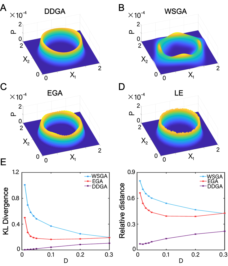
Figure 1: Landscape of planar cubic systems and comparison among different methods. (A-D) Landscape obtained from the DDGA (A), the WSGA (B), the EGA (C) and the LE (D), where the WSGA oscillates the most compared with the DDGA and the EGA. (E) Performance of these three approximation approaches. We calculate the posterior K-L divergence ($d_{\textbf{KL}}$) and relative distance ($d_{\textbf{RD}}$) between the DDGA (purple line), the WSGA (sky blue line), and the EGA (red line), respectively, with the LE individually, where both the indexes indicate that the DDGA performs much better than the other two, especially for the small diffusion coefficient. As the diffusion coefficient increases, the EGA, the high-order moment approach, does not perform significantly better than the origin WSGA.

For the first group of parameters $\lambda=2,\,m_{1}=-1.5,$ and $m_{2}=1.5$, we perform the methods of DDGA, WSGA, EGA, and LE respectively to get the steady-state probability distribution (Fig. 1A-D). The steady-state probability distributions produced by the four methods all look like Mexican hat around the limit cycle. The main features of the landscape structure by the WSGA deviate from the landscape by the LE, especially at the peaks on the limit cycle. The incompatibility between the two distributions is due to the fact that, to avoid the divergence in the WSGA, the MFA method ignores the non-diagonal elements. The non-diagonal elements affect the width of the Mexican hat where the direction of the limit cycle is not parallel to the coordinate. Losing the information on the non-diagonal elements may result in the inaccuracy of the width and then increase the number of the peaks. The distribution by the DDGA and the EGA both peak twice within an oscillation period (Fig. 1A, C), and the distribution by the DDGA are smoother than the distribution by the EGA. The DDGA method only relies on the first and second order information while the EGA method relies on the third-order information. When the third-order information is more volatile, the distribution by the DDGA is smoother than the distribution by the EGA.

The most direct conclusion from Fig. 1E is that the DDGA is the best among all these WSGA-based approaches, but there are also some interesting aspects to be noted. First, by pre-solving, the DDGA performs much better than the origin moments approaches such as the WSGA and the EGA under small noises. This is because that the diffusion is not obvious under small noises. Thus, the landscape almost surrounds the limit cycle, which makes the true solution closely tied to (almost directly relate to) the sub-distribution, i.e. the pre-solution, on the limit cycle. Although those moments approaches also consider the weighted summation to a certain extent, the weights are often set as constant values for simplicity. Meanwhile, our DDGA uses the pre-solution to obtain very accurate sub-distributions, which makes it perform exceptionally well under small noises.

Second, as mentioned in our previous work [22], the fitting effect of the WSGA and the EGA gradually get better with increasing noise intensity, since the limit distribution, when the noise increases to infinity, becomes a uniform distribution. At the same time, the EGA loses its efficacy under a larger noise, which is caused by the truncation error of the $\Omega$-expansion. Analogous to the “Runge phenomenon” in the polynomial interpolation, high-order approximation sometimes becomes less effective. The third phenomenon is that both the KL divergence and the relative distance between the DDGA and the LE increase as $D$ increases. This suggests that, for a larger noise, the DDGA may not fit as well as $D$ is sufficiently small. Notice that the DDGA is based on the hypothesis that the diffusion can be considered on the limit cycle first, and then towards the remaining normal plane locally. The second step relies on the $\Omega$-expansion and requires local stability towards the remaining plane. However, when the diffusion coefficient $D$ increases, the flux outside the neighborhood of the limit cycle may increase sufficiently large to break the assumption of local stability in the DDGA. Therefore, the DDGA method may not be as accurate as the case where $D$ is small. However, we can find that, even when $D$ increases sufficiently large, two measures indicate that in this planner cubic system, the DDGA still fits better than the WSGA and the EGA. Thus, the influence of the inaccuracy rising from the break of the assumption is limited. Our proposed pre-solution is still a useful tool for enhancing the approximating effect even when its mathematical assumption is partially dissatisfied. Simultaneously, the DDGA spends the least time in these approximation approaches as the time table listed in Supplementary Material, Table S1. We also choose another group of parameters, i.e. $\lambda=2,\,m_{1}=-0.5,$ and $m_{2}=1.2$, and obtain the similar conclusion (see details in Supplementary Material, Figure S1).

II.4.2 Application to synthetic oscillatory network

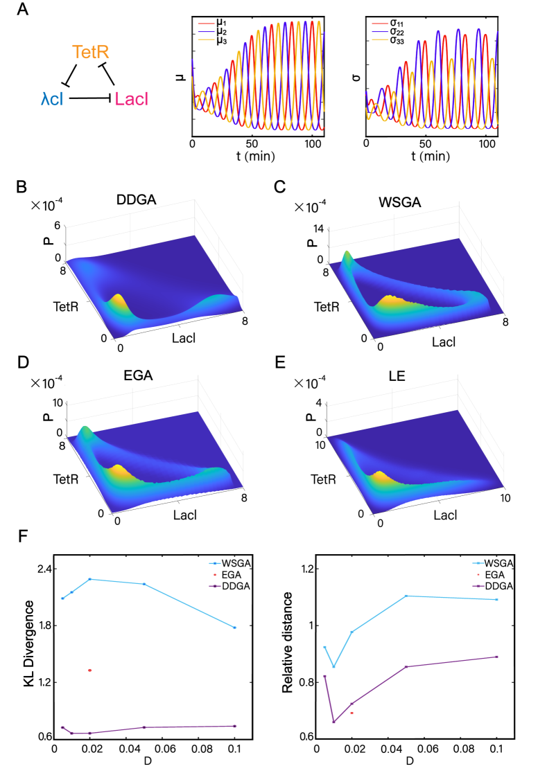
Figure 2: Landscape of synthetic oscillatory network and comparison using the methods of DDGA, WSGA and EGA with regard to the LE, respectively. (A) The negative feedback loop consists of three repressilators, LacI, TetR, and $\lambda$cI and their oscillating moments: mean and covariance. (B-E) Landscape obtained from the DDGA (B), the WSGA (C), the EGA (D), and the LE (E), where the DDGA is the only approach that can partially predict the “explosion phenomenon” of the LE. (F) Performance of these three approximation approaches. We calculate the posterior K-L divergence ($d_{\textbf{KL}}$) and the relative distance ($d_{\textbf{RD}}$) between the DDGA (purple line), the WSGA (sky blue line), and the EGA (one red point, due to its extreme amount of spending time and calculation resources), with the LE individually. The DDGA and the EGA achieve almost the same efficacy, better than the WSGA.

To investigate the performance for the DDGA in those realistic biological systems, we apply the methods of DDGA, EGA, and WSGA to a genetic circuit. Elowitz and Leibler engineered a synthetic oscillatory network in Escherichia coli using three transcriptional repressor systems that do not belong to any endogenous biological clock. This engineered network periodically triggers the synthesis of green fluorescent protein [31](Fig. 2A). For the repressilators TetR, LacI, $\lambda$ cI, their concentrations, $p_{i}\,(i=\text{LacI},\,\text{TetR},\,\lambda\text{cI})$, and their corresponding mRNA concentrations, $m_{i}$ are governed by the following equations:

$$\begin{cases}\begin{aligned} \frac{\text{d}m_{i}}{\text{d}t}&=-m_{i}+\frac{\alpha}{1+p_{j}^{n}}+\alpha_{0},\\ &(i,j)=(\text{LacI},\lambda\text{cI}),\,(\text{TetR},\text{LacI}),\,(\lambda\text{cI},\text{TetR}),\end{aligned}\\ \begin{aligned} \frac{\text{d}p_{i}}{\text{d}t}=-\beta(p_{i}-m_{i})\,,\,i=\text{LacI},\,\text{TetR},\,\lambda\text{cI}.\end{aligned}\end{cases}$$

Here, we select parameters as $n=2,\,\alpha=10,\,\alpha_{0}=0.01$ and $\beta=0.5$ and apply the methods of DDGA, EGA, and WSGA to this synthetic oscillatory network (Table S4 in Supplementary Material). As such, following the MFA or the DDGA procedure, the moments oscillate periodically (Fig. 2A), while the probability looks like a Mexican hat with a triangle-like limit cycle. We emphasize that the EGA approach is constructed by the multi-dimensional integral which spends about $10^{3}$ times than the WSGA as the dimension becomes higher. In this system, an implementation of EGA costs about 270 hours that cannot be performed generally, while that of the WSGA based on the MFA only spend 40 minutes (the origin WSGA without using the MFA may cost $10^{2}$ times than MFA, too). Simultaneously, the DDGA approach only costs about 10 seconds by simplifying the ODEs into the matrix equations, so that the DDGA comprehensively and significantly improves the WSGA in terms of the accuracy and the computational cost as well. In simulation we discover an abnormal phenomenon. Particularly, when the diffusion coefficient $D$ becomes larger, the “Mexican-hat-like” landscape loses its shape. The landscape almost disappears around the diagonal leg of the limit cycle, and “explodes” into the inside area of the limit cycle. As such, we only implement these approaches for the diffusion coefficient no more than $10^{-1}$.

When $D=0.02$ in Fig. 2E, we discover that the landscape partially disappears around the diagonal leg of the limit cycle, and overflows towards the insides of the limit cycle. This explosion phenomenon causes the inefficacy of almost every approximate approach, because none of them can predict the disappearance of the limit cycle in a periodic system. However, our pre-solution in the DDGA partially captures this abnormal phenomenon (Fig. 2B, F). We also calculate the KL divergence $d_{\textbf{KL}}$ and the relative distance $d_{\textbf{RD}}$ between these approximate approaches and Langevin simulation, as shown in Fig. 2F. Under $D=0.02$, where we obtain the only one data of the EGA, we find that the DDGA and the EGA improve the WSGA in different aspects, and they outweigh the other in one of the measure indices. As the dimension increases, the efficiency of MFA’s approximation also increases, which makes the origin approximate approaches such as the WSGA and the EGA more appropriate. At the same time, the DDGA describes the explosion phenomenon by pre-solving, and reaches almost the same efficiency as the EGA in about $10^{-5}$ times of the computational cost of the EGA (Table S1 in Supplementary Material). We explore the WSGA and the DDGA for different diffusion coefficients, as shown in Fig. 2F where the DDGA performs significantly better than the WSGA, while the explosion phenomenon influences these approaches indeed.

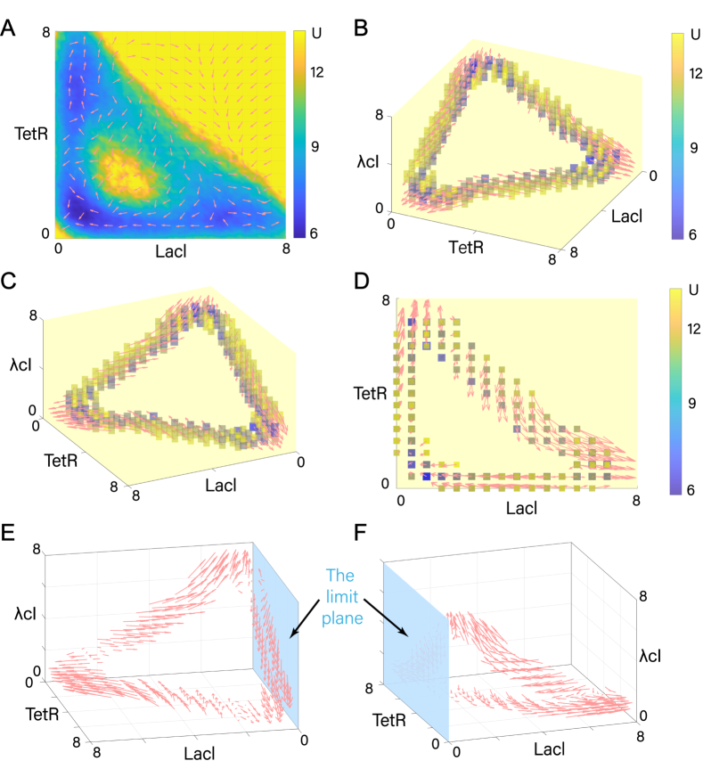
Figure 3: Coexistence of the stability of the oscillation and the explosion of the landscape explained by the flux. (A) The landscape and the flux for the 2-dimensional projection. The flux in the diagonal leg pushes the landscape into the inside. (B-D) The landscape and the flux for the 3-dimensional projection spanned by the concentration of the three mRNAs. The arrows represent the flux, while the color of the small rectangles represents the potential at these points. We only display the landscape and the flux in the neighborhood of the limit cycle to describe evolution around the limit cycle. In the 3-dimensional projection, the symmetry of the system can be recognized, and we find a curl field around the limit cycle. (E-F) Two views of the limit planes where the concentration of one of the mRNAs equals to zero (we only highlight one limit plane in blue). In this system, the three limit planes restrict the flux and push the landscape back to the neighborhood of the limit cycle.

To further explore the explosion phenomenon, we display the landscape and the flux (see details in Methods) for the 2-dimensional projection in Fig. 3A. We notice that the flux around this region also pushes the landscape into the insides. This lays the foundation for the explosion phenomenon. We further check the second-order information of the dynamics around the explosion point, and find that the Jacobian matrix $\boldsymbol{A}$ in Eq. 2 loses the negative-definite properties towards the direction of the limit cycle and one other orthogonal direction. The absence of negative-definite properties in the orthogonal direction impairs the local stability of the limit cycle in that specific orthogonal orientation. Consequently, this leads to the flux driving the landscape to overflow from the limit cycle towards that orthogonal direction. Since our DDGA method highly relies on the second-order information, the explosion is partially captured by our method. Therefore, the landscape by the DDGA also exhibits some explosion in the diagonal legs of the limit cycle. This explains why our method achieves similar excellence when the diffusion coefficient becomes large. This is essentially different from the case in the planar cubic systems.

We have found the explosion phenomenon around the diagonal region of the limit cycle in the projected 2-dimensional space. However, the synthetic oscillatory network has been fully studied and the stability of the oscillation has been verified. Intuitively, this seems contradictory to the “explosion” of the landscape, which indicates that our projection to 2-dimensional subspace loses some “resilience information” to overcome the explosion. To illustrate how both phenomena occur, we display the landscape and the flux in the 3-dimensional projection (Fig. 3B-D) spanned by the concentration of the three mRNAs. We find that there is a strong curl field around the limit cycle and the three limit planes, where the concentrations of the three mRNAs equal to zero separately, restricting the area of the dynamics. For the 2-dimensional surface, the flux flows into the limit cycle, but for the higher dimensions the curl field pushes the flux cycling around the limit cycle.

When the diffusion coefficient is small, the trajectories almost follow the dynamical drift force and curl around the limit cycle. Since in the three legs of the limit cycle, there is a concentration of the mRNAs close to zero, the trajectories finally reach a corresponding limit plane (Fig. 3E, F) and then are pushed back to the limit cycle, maintaining the stable property of the oscillation. The larger the diffusion coefficient be, the larger the probability of escaping towards the inside or even cross the limit plane around the curling. This results in an explosion of the landscape, which explains the coexistence of the stability of the oscillation and the explosion for the landscape. Moreover, we notice that due to the symmetry of systems, the explosion of the landscape will happen for all three legs of the limit cycle. Meanwhile, for the projection of the landscape into 2-dimensional subspace, the explosion in the non-diagonal legs, integrated by the projection, becomes not that obvious. The high-dimensional flux explains the abnormal phenomenon in the low-dimensional landscape, showing that an appropriate projection to lower dimension can preserve more information about the high-dimensional dynamics.

II.4.3 Application to a high-dimensional mammalian cell cycle network

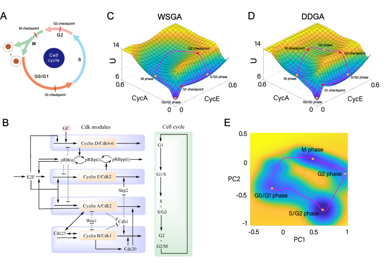
Figure 4: Landscape of the mammalian cell cycle network. (A) An illustration for complete progress of the cell cycle in mammalian cells. (B) The wiring diagram of the cell cycle network. The network includes four major cyclin/Cdk complexes centered on cyclin D/Cdk4-6, cyclin E/Cdk2, cyclin A/Cdk2, and cyclin B/Cdk1, controlling the four stages of cell cycle. (C-D) The landscape of the cell cycle network constructed by the WSGA (C) and the DDGA (D). The landscape by the WSGA shows three basins and two checkpoints, while the landscape by the DDGA shows one more basin and one more checkpoint, which is more consistent with the biological knowledge. (E) The landscape is shown in the reduced dimensions, where four significant phases are displayed. The contribution rates of PC1 and PC2 are $32.18\%$ and $24.56\%$, respectively.

We further apply these approaches to a high-dimensional mammalian cell cycle model, investigating the performance of the DDGA and the WSGA [2, 3], since the EGA is almost ineffective due to the dimensional curse here. The cell cycle model is mainly determined by four central cyclin/Cdk complexes (Fig. 4B) which induces four cell cycle stages (G0/G1, S, G2 and M, Fig. 4A) [2]. This model comprises 44 variables, including these complexes, alongside key elements such as pRB (tumor suppressor), E2F (transcription factor) and GF (growth factor, a critical parameter controlling the oscillation of cell cycle). In essence, it describes the underlying dynamics governing cell cycle progression, emphasizing the pivotal roles of these central cyclin/Cdk complexes within the intricate regulatory network.

Potential energy landscape provides a powerful tool to investigate the dynamical behavior of this mammalian cell cycle, Li et al. proposed that on the landscape obtained by WSGA, the emergence of three local basins and two saddle points along the limit cycle trajectory can reflect the different phases of the cell cycle progression and the checkpoints of phase transition (G1 checkpoint and S/G2 DNA replication checkpoint) [3]. In this work, more biological properties can emerge from the landscape using the DDGA approach. The dynamics of this model is governed by a 44-dimensional ODEs based on the Michaelian kinetics (see details in Supplementary Material). We choose as GF=0.5 where the system oscillates, and the diffusion coefficient as $D=0.05$ to test whether the DDGA improves the WSGA. (The other parameters we choose is listed in Table S5, Supplementary Material.) As we claim, the computational cost of the WSGA significantly increases as the dimension becomes higher, for a large amount of ODEs’ computation, while the DDGA costs much less (Table S1 in Supplementary Material). We apply both the WSGA and the DDGA to the system, and both methods characterized the landscape as a Mexican hat with multiple basins (Fig. 4C, D). In both landscapes, the deepest basin is centered around the origin point, with a substantial barrier traversing the limit cycle on the right side. The landscape resulting from the WSGA exhibits three basins that correspond to the G0/G1, the S/G2, and the M phases, along with two checkpoints: the G1 checkpoint and the G2 checkpoint. The most prominent barrier, housing the G2 checkpoint, separates the S/G2 and the M basins.

Some conspicuous observation emerges in the landscape using the DDGA. An additional basin associated with the G2 phase is identified, and a new saddle point emerges along the new barrier brought by the additional basin. Moreover, the S/G2 phase basin on the DDGA landscape exhibits significantly greater depth than its counterpart (S/G2 phase) on the WSGA landscape. The new saddle point in the landscape aligns with the M check points. The emergence of the new basin now divides the M phase in the WSGA landscape into two phases: the M phase and the G2 phase, and the biggest barrier instead separates the G2 phase and the S/G2 phase. The significant difference may rise from the two improvements in our methods: The pre-solution and the diffusion in the normal plane. To see how the additional basin appears, we first focus on the origin of the three basins in the WSGA landscape. In the WSGA approaches, the weight function, i.e. the pre-solution, is taken to be constant. The three basins arise from the significantly large covariance in the their positions, which also corresponds to the three local maxima of the covariance. In the DDGA approaches, the weight function (pre-solution) is introduced, and two local maxima of the pre-solution corresponding to the G2 phase and the S/G2 phase basins are found. The additional basin and greater depth of the S/G2 basins are attributed of this pre-solution. This implies that the peeks of pre-solution also contributes to the formation of the basins by capturing the tangent dynamics along the limit cycles.

Additionally, we incorporate the dimension reduction technique developed by Kang and Li into our landscape analysis conducted through DDGA [32]. In this approach, since the landscape consists of some Gaussian distributions, the covariance matrix is calculated from the mean and covariance of these Gaussian distributions, and then decomposed through the module of its eigenvalues. Then several eigenvectors $\omega_{1},\dots,\omega_{k}$ with the largest eigenvalues are chosen to be the projection direction. Finally, $(z_{1},\dots,z_{k})^{\top}=(\omega_{1}^{\top}\boldsymbol{x},\dots,\omega_{k}^{\top}\boldsymbol{x})^{\top}$ is defined to be the projection variables which display the most important information of the system (see details in Methods). In the mammalian cell cycle network, we choose $k=2$ and obtain the first two principal components of the landscape with the contribution rates $32.18\%$ and $24.56\%$, and the top five genes having major contributions to PC1 include Cdc45, Pol, Pbi, Me, and Pai (Table S2 in Supplementary Material). We display the projection of the energy landscape into these two components (Fig. 4E). The projection facilitated by the two components are also beneficial distinguishing the four phases in the cell cycle.

III Conclusion

In this article, we introduce an efficient and effective approximation approach, named as DDGA, for quantifying the energy landscape of periodic oscillatory networks. We extend the application of this approach to various gene regulatory networks of diverse dimensions. Moreover, we delve deeper into the mathematical interpretation of the “explosion” of covariance and enhance the theoretical foundation of the WSGA-based approaches. Our approach involves several steps. First, we provide a pre-solution which is a distribution on the limit cycle, a low-dimensional stable manifold, to capture the low-dimensional dynamics and provide a comprehensive overview of the oscillation structure. This pre-solution is obtained by deriving and solving the FPE constrained to the limit cycle. It significantly promotes the precision of the weighted function in the WSGA. Subsequently, we incorporate diffusion effects based on the WSGA framework. We establish that the diffusion process on the orthogonal normal plane of the limit cycle can be approximated as a stationary process, simplifying a majority of ODEs into matrix equations. As a result, computation for the covariance matrix is substantially expedited. Our DDGA dissects the stochastic evolution into the tangential and the orthogonal directions, effectively reconciling the trade-off between excluding non-diagonal covariance terms and avoiding “covariance explosion”.

To showcase the advantages of the DDGA, we evaluate its performance on three distinct oscillatory systems of dimension 2, 6, and 44, respectively. Through two probability measure indices and time-cost analysis, we benchmark the DDGA against two widely-used methods, the WSGA and the EGA. The results suggest that our new approach facilitates the improved quantification of the landscape for the periodic oscillatory systems, especially when the diffusion coefficient is not significantly large. The DDGA also promotes the explanations of intricate biological mechanisms. For example, it identifies the explosion phenomenon in the 6-dimensional synthetic oscillatory network and detects new basins and checkpoints that the original WSGA fails to discern in the 44-dimensional mammalian cell cycle network. These findings underline the DDGA as a valuable tool to effectively quantify oscillatory dynamics. To better elucidate the phenomena predicted by DDGA, we employ the flux and the limit planes in synthetic oscillatory networks to unravel the coexistence of the explosion phenomenon and the stability of the limit cycle. In conclusion, our approach presents a useful tool for studying stochastic and periodic dynamics by quantifying the associated energy landscape.

IV Methods

IV.1 Method: Calculating potential landscape using higher-dimensional moments

The EGA extends the moment approaches based on the WSGA [22]. Bian et al. derived the equations satisfying the third moments/the skewness tensor $\varPhi$ of the system as:

$$\dot{\phi}_{ijk}(t)= \sum\limits_{l=1}^{n}\left[\frac{\partial F_{i}(\boldsymbol{\mu}(t))}{\partial x_{l}(t)}\phi_{jkl}(t)+\frac{\partial F_{j}(\boldsymbol{\mu}(t))}{\partial x_{l}(t)}\phi_{kil}(t)\right.$$

$$+ \left.\frac{\partial F_{k}(\boldsymbol{\mu}(t))}{\partial x_{l}(t)}\phi_{ijl}(t)\right]\,,\,1\leq i,j,k\leq n.$$

The relationship between the first three moments and the probability distribution is connected by a special characteristic function and the Fourier transformation:

$$\begin{cases}\begin{aligned} \boldsymbol{f}(y_{1},y_{2},\dots,y_{n})=&\exp\left\{\text{i}\left\langle\boldsymbol{\mu},\boldsymbol{y}\right\rangle_{\mathbb{E}}+\frac{\text{i}^{2}}{2!}\left\langle\boldsymbol{\Sigma},(\boldsymbol{y}\otimes\boldsymbol{y})\right\rangle_{\mathbb{E}}\right.\\ +&\left.\frac{\text{i}^{3}}{3!}\left\langle\boldsymbol{\Phi},(\boldsymbol{y}\otimes\boldsymbol{y}\otimes\boldsymbol{y})\right\rangle_{\mathbb{E}}\right\}\end{aligned}\\ \begin{aligned} &\boldsymbol{\rho}(x_{1},x_{2},\dots,x_{n}):=\\ &\frac{1}{(2\pi)^{n}}\iint\dots\int\exp\{-\text{i}\left\langle\boldsymbol{y},\boldsymbol{x}\right\rangle_{\mathbb{E}}\}\boldsymbol{f}(y_{1},\dots,y_{n})\text{d}y_{1}\dots\text{d}y_{n},\end{aligned}\end{cases}$$

where $\boldsymbol{f}$ is the characteristic function contains the first three moments $\boldsymbol{\mu},\,\boldsymbol{\Sigma}$, and $\boldsymbol{\Phi}=D^{\frac{3}{2}}\cdot(\phi_{ijk})$, and $\boldsymbol{\rho}$ represents its corresponding probability.

IV.2 Method: Calculating the low-dimensional flux through FPE

Review that the general FPE is formulated as

$$\nabla(\boldsymbol{F}(\boldsymbol{x})\rho(\boldsymbol{x})-\nabla(\boldsymbol{d}(\boldsymbol{x})\rho(\boldsymbol{x})))=0.$$

This rises from the law of the probability conservation:

$$\boldsymbol{J}(\boldsymbol{x}) =\boldsymbol{F}(\boldsymbol{x})\rho(\boldsymbol{x})-\nabla(\boldsymbol{d}(\boldsymbol{x})\rho(\boldsymbol{x})),$$ (10)

$$\nabla\cdot\boldsymbol{J}(\boldsymbol{x}) =0.$$

Thus, if we get the steady probability distribution $\rho(\boldsymbol{x})$, the origin flux $\boldsymbol{J}(\boldsymbol{x})$ can be calculated by Eq. 10. Since $\boldsymbol{F}(\boldsymbol{x})=\frac{\nabla(\boldsymbol{d}(\boldsymbol{x})\rho(\boldsymbol{x}))}{\rho(\boldsymbol{x})}+\frac{\boldsymbol{J}(\boldsymbol{x})}{\rho(\boldsymbol{x})}$, the driving force $\boldsymbol{F}(\boldsymbol{x})$ of the system is decomposed to two terms: One is from the energy landscape, and the other is from the probability flux $\boldsymbol{J}(\boldsymbol{x})$.

To get the flux in the 2-dimensional projection plane, we implement some dimension reduction approaches. Note the limit cycle as $C=\{x(s):s\in[0,1]\}$, and get the segmentation of $C$ as $x_{i}=x(\frac{i}{n}),(1\leq i\leq n)$. Given two orthonormal directions $u_{1,2}\in\mathbb{R}^{N}$, such as the two variables of the system, or the first two principle components in the dimension reduction approach [32], we then get the ordinary least square (OLS) surface of the limit cycle by

$$L_{\text{ols}}:\,A_{\text{ols}}\begin{pmatrix}u_{1}\\ u_{2}\\ 1\end{pmatrix}=\boldsymbol{0},$$

where

$$A_{\text{ols}}^{3\times 3} =\begin{pmatrix}z_{1}&z_{2}&b\end{pmatrix}=(X^{\top}X)^{-1}X^{\top}Y,$$

$$X^{n\times 3} =\begin{pmatrix}u_{1}&u_{2}&e\end{pmatrix},$$

$$Y^{n\times 2} =A\begin{pmatrix}x_{1}&x_{2}&\cdots&x_{n}\\ 1&1&\cdots&1\end{pmatrix}^{\top},$$

$$e^{n\times 1} =(1,1,\cdots,1).$$

Thus the 2-dimensional flux in the OLS surface spanned by $u_{1,2}$ is formulated as

$$J(y_{1},y_{2})=\begin{pmatrix}v_{1}&v_{2}\end{pmatrix}^{\top}\boldsymbol{J}\left(A_{\text{ols}}\begin{pmatrix}u_{1}\\ u_{2}\\ 1\end{pmatrix}\right).$$

IV.3 Method: Complementing the covariance matrix in multistable systems

The second moment ODEs of the covariance matrix Eq. 2 can be transformed into linear ODEs by the Kronecker product. Particularly, for any $n\times n$ matrix $B=(\vec{b_{1}},\dots,\vec{b_{n}})$, if we denote $\text{vec}(B):=(\vec{b_{1}}^{\top},\dots,\vec{b_{n}}^{\top})^{\top}$ as a $n^{2}\times 1$-vector, we can transform the covariance ODEs into (see detail in Supplementary Material)

$$\dot{\text{vec}(\Sigma)}=(I\otimes\boldsymbol{A}+\boldsymbol{A}\otimes I)\text{vec}(\boldsymbol{\Sigma})+D\Big{[}\text{vec}(\boldsymbol{d})+\text{vec}(\boldsymbol{d}^{\top})\Big{]}.$$

Through Lyapunov’s stability criterion, the solution is asymptotically stable if and only if the real parts of the evolution matrix’s eigenvalues are all negative. Thus, in the WSGA-based approach, a critical condition for the Jacobian matrix $\boldsymbol{A}$ becomes: All the eigenvalues of $(I\otimes\boldsymbol{A}+\boldsymbol{A}\otimes I)$ are negative.

In Kang et al.’s approach [20], when the multistable systems evolve to its steady states, the moments (the mean and the covariance) will tend to constants as

$$\begin{cases}\begin{aligned} F(\boldsymbol{\mu}(+\infty))=0\end{aligned}\\ \begin{aligned} &\boldsymbol{\Sigma}(+\infty)\boldsymbol{A}^{\top}(+\infty)+\boldsymbol{A}(+\infty)\boldsymbol{\Sigma}(+\infty)\\ &+D\Big{[}\boldsymbol{d}(\boldsymbol{\mu}(+\infty))+\boldsymbol{d}^{\top}(\boldsymbol{\mu}(+\infty))\Big{]}=0.\end{aligned}\end{cases}$$

This kind of matrix equations can be simplified by the Kronecker product mentioned above. Specifically, the covariance ODEs are changed into

$$(I\otimes\boldsymbol{A}+\boldsymbol{A}\otimes I)\text{vec}(\boldsymbol{\Sigma})=-D\Big{[}\text{vec}(\boldsymbol{d})+\text{vec}(\boldsymbol{d}^{\top})\Big{]}.$$

where $\otimes$ represents the Kronecker product. Finally, $\boldsymbol{\Sigma}$ can be solved out in terms of $\text{vec}(\boldsymbol{\Sigma})$ through a matrix multiplication:

$$\text{vec}(\boldsymbol{\Sigma})=-D(I\otimes\boldsymbol{A}+\boldsymbol{A}\otimes I)^{-1}\Big{[}\text{vec}(\boldsymbol{d})+\text{vec}(\boldsymbol{d}^{\top})\Big{]}.$$