Universal Modelling of Emergent Oscillations in Fractional Quantum Hall Fluids

Abstract

Density oscillations in quantum fluids can reveal their fundamental characteristic features. In this work, we study the density oscillation of incompressible fractional quantum Hall (FQH) fluids created by flux insertion. For the model Laughlin state, we find that the complex oscillations seen in various density profiles in real space can be universally captured by a simple damped oscillator model in the occupation-number space. It requires only two independent fitting parameters or characteristic length scales: the decay length and the oscillation wave number. Realistic Coulomb quasiholes can be viewed as Laughlin quasiholes dressed by magnetorotons which can be modeled by a generalized damped oscillator model. Our work reveals the fundamental connections between the oscillations seen in various aspects of FQH fluids such as in the density of quasiholes, edge, and the pair correlation function. The presented model is useful for the study of quasihole sizes for their control and braiding in experiments and large-scale numerical computation of variational energies.

Introduction.— Characteristic density oscillations in the presence of perturbations are a fundamental aspect of quantum fluids. For the Fermi liquid, the long-range Friedel oscillation in the presence of impurity is a direct consequence of the existence of Fermi surface and quasiparticle excitations [1]. Similarly, for the non-Fermi liquids which go beyond the Fermi liquid paradigm (e.g. the Luttinger liquid [2], composite fermion liquid [3], quantum Hall liquid [4, 5] and strange metal [6]), characteristic density oscillations manifest as spin-charge separation [7], charge-vortex duality [8], anomalous decay laws and exponents [9, 10, 11, 12, 13], and so on. Understanding and accurately modeling such oscillations, which are of both theoretical and experimental significance, remains an outstanding open problem.

An important class of non-Fermi liquids is the incompressible fractional quantum Hall (FQH) fluids which display characteristic oscillatory features that encode both geometric and universal topological information. When a quantum of flux is inserted into the uniform FQH ground state, quasiholes carrying a fractional charge [14] and obeying fractional statistics [15] are created. They also carry a dipole moment to balance the Hall viscosity in the presence of the electric field gradient, which is proportional to the FQH topological shift [16]. The dipole moment, a characteristic feature of incompressibility, is established from the density oscillation at the edge [17]. Moreover, when an appropriate number of fluxes equivalent to removing an electron is inserted at the same position, the density of the bound state of a few stacked quasiholes is proportional to the pair-correlation function of the ground state [18]. In the limit of an infinite number of fluxes inserted, a macroscopic FQH edge is created, near which the density oscillation has been intensively studied [19, 18, 20, 21, 17, 22, 23, 24, 25, 26]. The FQH quasiholes, ground state pair-correlation function, and the QH edge can thus be understood as special cases of flux insertion (see Fig. 1) and are thus closely related. The precise underlying connections and both the qualitative and quantitative aspects of such oscillations, however, are not well understood.

In this Letter, we show that the real space density oscillation from the flux insertion in the model Laughlin state can be accurately modeled by a simple damped oscillation with degrees of freedom within a single Landau level (LL). The oscillation is determined by two characteristic length scales: the decay length and the oscillation wave number, and these serve as the only fitting parameters of the model. In contrast to previous works that directly model the real space density [27, 20, 21, 28, 22, 11, 12, 25, 29], we emphasize that the model should only focus on the guiding center degrees of freedom (within a single LL), as those are the relevant coordinates for any FQH phase. For the model Laughlin state, we study its quasihole, edge, and pair-correlation function using the aforementioned model-based approach treating them all on an equal footing. A phenomenological model for the damped oscillation of Laughlin quasiholes is proposed at general fillings. For the more realistic Coulomb interaction, where quasiholes are dressed by neutral excitations, a generalized damping model with four characteristic lengths is shown to work very well, which is useful for both numerical computations and experimental manipulation of quasiholes. Moreover, we find this generalized model also gives an accurate description of quasiholes in some of the composite fermion and non-Abelian topological phases.

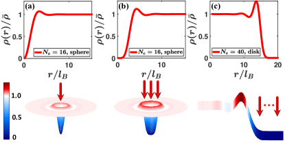
Figure 1: Schematic plot of excitations created by flux insertion at $\nu{=}1/3$. From left to right, the Laughlin quasihole obtained by insertion of a single flux (a), $3$-Laughlin quasiholes obtained by insertion of three fluxes (b), whose density is proportional to the ground state pair-correlation function, and the Laughlin edge obtained from the insertion of an infinite number of fluxes (c). The top panels show the density distribution $\rho(r)/\bar{\rho}$ in the radial direction, where $\bar{\rho}$ is the uniform background density. Panels (a) and (b) show results for $N_{e}{=}16$ on the sphere while panel (c) is for $N_{e}{=}40$ on the disk.

Universal damped oscillation.— The model wave function of the Laughlin quasihole located at the origin of the disk geometry for $N_{e}$ electrons is $\Psi_{L}^{1{-}\text{qh}}{=}\left(\prod_{i{=}1}^{N_{e}}z_{i}\right)\Psi_{L},$ where $\Psi_{L}{=}\prod_{1{\leq}i{<}j{\leq}N_{e}}(z_{i}{-}z_{j})^{m}e^{-\frac{1}{4}\sum_{i{=}1}^{N_{e}}|z_{i}|^{2}}$ is the Laughlin wave function at $\nu{=}1/m$ [14], $z_{i}{=}x_{i}{-}iy_{i}$ is the position of the $i^{\text{th}}$ electron, and the magnetic length at magnetic field $B$ is taken as the unit of length i.e., we set $l_{B}{=}\sqrt{\hbar c/(eB)}{=}1$. We can also stereographically map this state to the spherical geometry [30]. The density distribution of a single Laughlin quasihole at $\nu{=}1/3$ in the spherical geometry is shown in Fig. 2(a). Directly finding a simple empirical model for the real-space density distribution of quasiholes is challenging as the real-space structure is a mixture of the trivial LL (cyclotron) and the non-trivial FQH (guiding-center) contributions. A real-space density distribution $\rho(r)$ can be decomposed as $\rho(r){=}\sum_{i{=}0}^{N_{\phi}}n_{i}\rho_{i}(r)$, where $n_{i}$ is the average occupation number of the $i^{\text{th}}$ orbital, $\rho_{i}$ is the density computed from single-particle wave functions, and $N_{\phi}$ is the number of fluxes threading the sample. Only $n_{i}$ is related to the correlated FQH physics.

The Laughlin quasihole density exhibits damped oscillations in the occupation-number space [see Fig. 2(b)]. We take the real space position of each orbital as the arc distance from the north pole to the center of the $i^{\text{th}}$ equal-area slice of the sphere, i.e., $x_{i}{=}R\theta_{i}{=}\sqrt{N_{\phi}/2}\arccos\left[1{-}\left(1{+}2i\right)/N_{o}\right],$ where $R{=}\sqrt{N_{\phi}/2}$ is the radius of the sphere, $N_{o}{=}N_{\phi}{+}1$ is the number of orbitals on the sphere, and we index the orbitals from the north to the south pole by $k{=}0,1,\ldots,N_{\phi}$. We find the occupation-number oscillation of quasihole density $\delta n_{i}{=}n_{i}{-}\bar{n}$ [with $\bar{n}{=}(N_{e}{+}1/m)/N_{o}$ being the average background occupation] can be accurately captured by the following model:

$$\delta n_{i}=A_{1}\sin[k_{1}(x_{i}-x_{1})]\exp\left(-x_{i}/\lambda_{1}\right),$$ (1)

where $k_{1}$ and $\lambda_{1}$ are the oscillation wave number and decay length respectively, $A_{1}$ is the amplitude and $x_{1}$ is the zero point. The fitted result (red crosses) agrees almost perfectly [31] with the exact occupations (blue circles) as shown in Fig. 2(b). Correspondingly, the exact and fitted real-space density distributions are also nearly indistinguishable from each other as shown in Fig. 2(a).

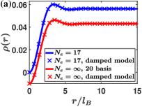
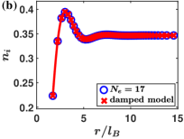
Figure 2: (a) The density distribution of a Laughlin quasihole located at the north pole of a sphere as a function of the arc distance $r$. The blue line and crosses denote the exact distribution and the fitting with our damped model [Eq. (1)], respectively for $N_{e}{=}17$. The red line and crosses denote the thermodynamic limit obtained from the polynomial expansion method [29] and our fitting [31], respectively, and the data points are shifted down by $0.01$ for clarity. (b) The occupation-number density. Blue circles and red crosses denote the exact density and that obtained from fitting with our model, respectively. The fitted curve is $n(r){=}0.68\sin[1.43(r{-}2.31)]\exp({-}r/1.21){+}\bar{n}$ with $\bar{n}{=}(N_{e}{+}1/3)/N_{o}$ with $N_{o}{=}50$.

It is important to note that the accurate fitting is achieved with only two independent fitting parameters $k_{1}$ and $\lambda_{1}$. The other two parameters in Eq. (1), $A_{1}$ and $x_{1}$, are fixed by the total charge $\sum_{i{=}0}^{N_{\phi}}\nu_{i}{=}N_{e}$ and the total angular momentum $\sum_{i{=}0}^{N_{\phi}}\nu_{i}(i{-}N_{\phi}/2){=}N_{e}/2$. The two conditions are equivalent to the constraints that a single quasihole has a charge $e_{1{-}\text{qh}}{=}{-}1/m$ and a dipole moment $d_{1{-}\text{qh}}{=}(1{-}1/m)/2$ in the thermodynamic limit; with both being topological and thus robust against perturbations. From finite-size-scaling, we find the following values of the parameters in the thermodynamic limit [31]:

$$k_{1}^{(1)}=1.38,\lambda_{1}^{(1)}=1.17,$$ (2)

where the superscript denotes the number of quasiholes. In contrast, if one works with the real-space density which includes the extra Landau orbit contribution, one has to introduce several tens of fitting parameters using the polynomial expansion method to capture the whole profile as done in Refs. [27, 29]. Furthermore, the important property that the Laughlin quasihole has a unique decay length and oscillation period is not easy to discern from real-space studies  [28].

Stacked Laughlin quasiholes.— The damped oscillation model can also be applied to $n$-stacked quasiholes created by inserting $n$ fluxes at the same location. The real-space density of such quasiholes gets increasingly complex with increasing $n$. Even for IQH fluid, the $n$-stacked holes have $\delta\rho(r){=}{-}1/(2\pi)\exp\left({-}r^{2}/2\right)(\sum_{i{=}0}^{n{-}1}r^{2i}/2^{i}i!)$, which is no longer a simple Gaussian distribution for $n{>}1$. Focusing on the FQH system with multiple quasiholes, we again look at its occupation-number density which reveals interesting physics and is no more complex even for $n{>}1$. The values of the characteristic lengths $k_{1}^{(n)}$ and $\lambda_{1}^{(n)}$ for different values of $n$ are shown in Figs. 3(a) and 3(b), where both $k_{1}^{(n)}$ and $\lambda_{1}^{(n)}$ increase as $n$ gets larger. The complicated real-space densities can be easily restored with the single-particle wave functions.

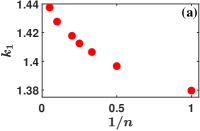
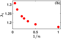
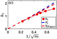
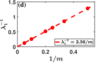
Figure 3: Top panels (a) and (b) show the characteristic lengths $k_{1}$ and $\lambda_{1}$ of Laughlin $n$-quasihole state at $1/3$. Bottom panels (c) and (d) show results for a single Laughlin quasihole at different fillings $\nu{=}1/m$. The red dashed line in (c) is the wave number of the Wigner crystal at the corresponding filling, and the blue dashed line denotes the intrinsic wave number $k^{\prime}_{1}{=}\sqrt{k_{1}^{2}{+}\lambda_{1}^{{-}2}}$ (see text).

The $m$-stacked quasihole at $\nu{=}1/m$ deserves special attention because its density distribution is proportional to the pair-correlation function of the Laughlin ground state. The density distribution of $m$-Laughlin quasiholes is $\rho(r){=}\mathcal{N}_{1}\int\prod_{i{=}2}^{N_{e}^{\prime}}d\bm{r}_{i}|\Psi_{L}^{m{-}\text{qh}}(\bm{r},\bm{r}_{2},{\ldots},\bm{r}_{N_{e}^{\prime}})|^{2},$ where $\mathcal{N}_{1}$ is a constant. On the other hand, the pair-correlation function $g(r){=}\mathcal{N}_{2}\int\prod_{i{=}3}^{N_{e}}d\bm{r}_{i}|\Psi_{L}(0,\bm{r},\bm{r}_{3},{\ldots},\bm{r}_{N_{e}})|^{2}.$ By substituting the explicit wave function $\Psi_{L}$ and $\Psi_{L}^{m{-}\text{qh}}$ into the expression of $g(r)$ and $\rho(r)$, respectively, one can show that $\rho(r)$ is proportional to $g(r)$ when $N_{e}{=}N_{e}^{\prime}{+}1$. Therefore, the decay length of the density of $m$-stacked Laughlin quasiholes is equal to the correlation length $\lambda_{\text{cor}}$ between electrons:

$$\lambda_{\text{cor}}=\lambda^{(m)}_{1}.$$ (3)

Our result is thus useful for the large-scale numerical computation of ground-state variational energies. One can use our modeled $g(r)$ to calculate the per-particle variational energy of the Laughlin state in terms of any general interaction $V(r)$ through the formula $V{=}(\bar{\rho}/2)\int d^{2}\,\bm{r}V(r)[g(r){-}1]$ [32], where $\bar{\rho}$ is the average density. For the Coulomb interaction $V(r){=}1/r$, the calculated energy $V$ with our modeled $g(r)$ is $-0.4096$ for $\nu{=}1/3$ and $-0.3278$ for $\nu{=}1/5$ [31], which are very close to the conjectured thermodynamic values $-0.4098$ [33, 34] and $-0.3275(1)$ [35] obtained from the extrapolation of small-size exact diagonalization results and large-scale Monte Carlo calculations. Thus for other realistic interactions, the thermodynamic variational energies can now be computed very efficiently with our modeled $g(r)$[31]. Besides, our method does not suffer from the systemic error of the polynomial expansion method at small $r$ [29].

In the limit of $n{\rightarrow}\infty$, the corresponding “Laughlin quasihole” also deserves special attention as it represents the edge of the QH fluid. Its density profile can also be well-fitted with a damped model in the occupation-number space with the characteristic lengths being $k_{1}^{\text{edge}}{=}1.49$ and $\lambda_{1}^{\text{edge}}{=}1.51$ [31] which are just the limiting values of $n$-quasiholes as shown in Fig. 3.

Moreover, we can determine the characteristic length scales at general Laughlin fillings $\nu{=}1/m$ by fitting the density profile of a single quasihole with the damped model given in Eq. (1). The results are shown in Figs. 3(c) and 3(d). With increasing $m$, the oscillations become more pronounced. We find that the decay length is proportional to $m$, i.e., $\lambda_{1}^{(1)}{=}m/2.56$. Meanwhile, the oscillation wave number $k_{1}$ gradually approaches that of the Wigner crystal [36], i.e., $k_{\text{Wigner}}{=}2{\times}3^{{-}1/4}\sqrt{\pi m}{=}2.69\sqrt{m}$. This is consistent with a recent study, carried out in Ref. [25], of the density oscillations at the edge of the Laughlin state.

Given the near-perfect fitting of such a simple model with only two fitting parameters [31], we conjecture that the damped oscillation model captures the main features of the universal oscillations in the Laughlin FQH fluid, and in principle can be derived. While we are not able to accomplish that here, a phenomenological model for Laughlin quasiholes at general fillings can be proposed based on these results. We view the system as a damped oscillator with wave number $k^{\prime}_{1}{=}\sqrt{k_{1}^{2}{+}\lambda_{1}^{-2}}$ serving as the intrinsic “wave number” which is a little larger than the wave number of the Wigner crystal $k_{\text{Wigner}}$ for small $m$ [see Fig. 3(c)]. The damping results from a “frictional force” which is proportional to the density $\nu{=}1/m$. The differential equation that describes this system is

$$\left[\partial_{r}^{2}+2\lambda_{1}^{-1}\partial_{r}+k^{\prime 2}_{1}\right]\delta n(r)+\mathcal{O}(\delta n^{2})=0,$$ (4)

where $\mathcal{O}(\delta n^{2})$ denote terms that can potentially arise from non-linear effects which we ignore here. The linear solution of Eq. (4) is just our damped model given in Eq. (1). Note that the model proposed in Eq. (4) is different from that proposed in Eq. (23) of Ref. [21], which does not consider the damped term and assumes a different intrinsic wave number at the level of linear response. Deriving this simple model from the microscopic wave function and capturing the non-linear effects remains an open problem [21, 22].

Quasiholes for realistic interactions.— Going beyond the model Laughlin quasihole wave functions, the density profile of quasiholes from realistic interactions becomes more complicated, because such quasiholes are dressed by neutral excitations [37, 38]. Here we study the quasihole in the presence of the following tunable interaction

$$H_{\alpha}=(1-\alpha)V_{1}+\alpha V_{\text{Coulomb}},$$ (5)

where $V_{\text{Coulomb}}{=}1/r$ is the Coulomb interaction and $\alpha{\in}[0,1]$ is a tunable parameter. By varying $\alpha$, one can trace the evolution between the Laughlin quasihole ($\alpha{=}0$) and the Coulomb quasihole ($\alpha{=}1$). As $\alpha$ increases, the oscillations in the density of the quasihole become more pronounced and multiple periods/frequencies are observed. As a result, the single-damped model of Eq. (1) can no longer capture the whole density profile of the Coulomb quasihole. Instead, we need to generalize the model to include an additional damped oscillation that has a shorter range as shown in Fig. 4(a). The dependence of the characteristic lengths of the two modes on $\alpha$ is shown in Fig. 4(b). The wave number of the long-range mode $k_{1}$ is nearly unchanged and its decay length $\lambda_{1}$ becomes larger as $\alpha$ increases. This is not hard to understand, because the interaction becomes more long-ranged as $\alpha$ is increased. For the short-range mode, its wave number $k_{2}$ approaches $0$ as $\alpha{\rightarrow}0$ and it provides nearly no contribution to non-empty orbitals of Laughlin quasihole. This is consistent with the result that the Laughlin quasihole can be well-modeled with a single-damped oscillation.

Although the generalized model captures the density profile of the Coulomb quasihole accurately, one should be careful of issues about possible overfitting and strong finite size effects [see Ref.  [31] for a discussion of these]. Nevertheless, the high accuracy of the fitting suggests that the model captures at least two oscillation modes for the Coulomb quasihole. Our result quantitatively characterizes the deviation between the Coulomb and Laughlin quasiholes and reveals the non-universal effects induced by realistic interactions. This deviation arises from the dressing of the Laughlin quasihole by low-energy magnetoroton states [39, 37, 38]. Since the Coulomb quasihole and the Coulomb edge are closely related by flux insertion, the low-energy magnetoroton mode should also account for the deviation between the Coulomb edge and the Laughlin edge as observed in Refs. [24, 26]. Moreover, other non-universal effects away from the chiral Luttinger theory [10, 40, 41] can potentially be understood by studying the microscopic bulk quasihole [42], which requires much less computational efforts because its fluctuation and related non-linear effects are much smaller compared to the edge effects.

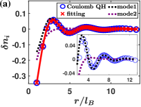
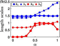
Figure 4: (a) Occupations of the Coulomb quasihole at $\nu{=}1/3$ for $N_{e}{=}14$ on the sphere. The fitted curve (red line) is the sum of the long-range $0.23\sin[1.48r{-}2.82]\exp({-}0.42r)$ (black dotted line) and the short-range $0.51\sin[0.54r{-}1.86]\exp({-}0.93r)$ (purple dotted line) modes. The inset is a zoom-in on the tail of the damped oscillations. (b) The dependence of characteristic lengths of the two modes on $\alpha$ [defined in Eq. (5)] for $N_{e}{=}14$. The blue and red colors denote the long-range and short-range modes respectively.

Quasiholes in Jain and non-Abelian phases.— The generalized damped oscillation model fails to capture the states in higher LLs where the interaction is long-ranged and the finite-size effects are very strong. Interestingly, the model continues to give a good description of Abelian quasiholes obtained from flux insertion (but no fractionalization) for many model QH fluids, including the Moore-Read [43, 44], Gaffnian [45], Fibonacci  [46], and composite fermion states at $\nu{=}2/5$ and $3/7$ [47, 32]. In addition to a very small fitting error, the modeled density profile is much smoother than those obtained from the polynomial expansion method. This is especially the case when the density profile in the real space looks irregular, for example in the case of pair-correlation of the Moore-Read state [31]. It is important to note that the finite-size scaling of the generalized model is not good suggesting potential over-fitting issues. This technical problem can be overcome by collecting data for larger system sizes by employing the density matrix renormalization group [48] and Monte Carlo method [26]. That would then allow for large-scale numerical computation of states beyond the simple Laughlin phases.

Summary.— We show the complex density oscillation of generic Laughlin $n$-quasiholes state in real space can be modeled by a simple damped oscillation in the occupation-number space. Moreover, the more realistic Coulomb quasihole can be well-fitted by a generalized damped oscillation model. The generalized model also applies to many other types of quasiholes. Our work paves the way to reveal the underlying connections between various oscillatory features of FQH fluids and the structure of quasiholes in the occupation-number space. It also provides an avenue to carry out large-scale numerical computations of ground-state variational energies. Determining the length scales of realistic quasiholes is crucial for designing experimental setups that can measure their fractional charge and statistics.

G. Ji thanks Nicolas Regnault, Ha Quang Trung, Yuzhu Wang, Greg J. Henderson, and Yayun Hu for valuable discussions. Some of the numerical calculations reported in this work have been carried out with the DiagHam package [49] for which we are grateful to its authors. Some of the numerical computations were done on the Nandadevi supercomputer, which is maintained and supported by the Institute of Mathematical Science’s High-Performance Computing Center. ACB thanks the Science and Engineering Research Board (SERB) of the Department of Science and Technology (DST) for funding support via the Mathematical Research Impact Centric Support (MATRICS) Grant No. MTR/2023/000002. This work is supported by the National Research Foundation, Singapore under the NRF fellowship award (NRF-NRFF12-2020-005).

Supplemental Material for “Universal Modelling of Emergent Oscillations in Fractional Quantum Hall Fluids”

The Supplemental Material contains the detailed numerical data of fitting parameters for the model $n$-Laughlin quasiholes at $\nu{=}1/m$, the Coulomb quasihole at $\nu{=}1/3$, and the pair-correlation function of Moore-Read state at $\nu{=}1/2$.

SI 1/3 Laughlin quasihole

We obtain the occupation number $n_{i}$ of a single Laughlin quasihole for $m{=}3$ and $N_{e}{=}10{-}17$ using Jack polynomials [50]. The parameters of the damped oscillatory model $\delta n_{i}{=}A_{1}\sin[k_{1}(x_{i}{-}x_{1})]\exp\left({-}x_{i}/\lambda_{1}\right)$ for the occupation-number $\delta n_{i}{=}n_{i}{-}\bar{n}$ are shown in Table  S1. The finite size scaling of the oscillation wave number and the decay length is shown in Fig. S1. They have an almost perfect linear scaling in $1/N_{e}$ allowing us to do the thermodynamic extrapolation reliably. Once the $n_{i}$ are determined, the real-space density of Laughlin quasihole in the thermodynamic limit is given by

$$\rho(r) =\sum_{i=0}^{\infty}n_{i}\rho_{i}(r),$$ (S1)

$$\rho_{i}(r) =\frac{1}{2\pi 2^{i}i!}r^{2i}\exp\left[-\frac{r^{2}}{2}\right].$$ (S2)

To check the accuracy of the model, we compare the density profile of the quasihole in the thermodynamic limit produced by our method and the polynomial expansion method proposed in Ref. [29]. The two methods deviate very slightly from each other (root-mean-square difference is $2{\times}10^{-5}$) producing nearly coincident curves as shown in Fig. 2(a). This implies that, even though our model is very simple with only two free parameters, our result is as accurate as the polynomial expansion method which uses several tens of parameters.

$N_{e}$	$A_{1}$	$k_{1}$	$k_{1}*x_{1}$	$1/\lambda_{1}$	$R^{2}$
10	0.6757	1.4734	3.3342	0.8051	0.999883
11	0.6774	1.4646	3.3305	0.8097	0.999893
12	0.6787	1.4574	3.3277	0.8133	0.999904
13	0.6799	1.4514	3.3253	0.8164	0.999910
14	0.6809	1.4462	3.3231	0.8191	0.999915
15	0.6819	1.4417	3.3211	0.8214	0.999918
16	0.6827	1.4377	3.3194	0.8234	0.999921
17	0.6835	1.4343	3.3178	0.8252	0.999923
$\infty$	0.6944	1.3785	3.2947	0.8538	0.999982

Table S1: Parameters of the damped oscillator model for the density of a single Laughlin quasihole at $\nu{=}1/3$ for $N_{e}$ electrons in the spherical geometry. The statistical measure $R^{2}$ is the coefficient of determination for how well the modeled occupation predicts the exact occupation numbers. The final row is the thermodynamic extrapolation result as a function of $1/N_{e}$.

$N_{e}$	$A_{1}$	$k_{1}$	$k_{1}*x_{1}$	1/$\lambda_{1}$	$R^{2}$
10	2.1345	1.5208	4.8670	0.7670	0.999885
11	2.1446	1.5109	4.8520	0.7720	0.999886
12	2.1514	1.5028	4.8402	0.7759	0.999885
13	2.1571	1.4961	4.8304	0.7792	0.999887
14	2.1625	1.4902	4.8219	0.7821	0.999888
15	2.1676	1.4851	4.8143	0.7846	0.999890
16	2.1724	1.4806	4.8076	0.7869	0.999891
$\infty$	2.2335	1.4138	4.7094	0.8198	0.999900

Table S2: Similar to Table  S1 except the parameters are for $3{-}$Laughlin quasiholes at $\nu{=}1/3$.

$N_{e}$	$A_{1}$	$k_{1}$	$k_{1}*x_{1}$	1/$\lambda_{1}$	$R^{2}$
20	5.2491e-04	1.5436	12.5625	0.6400	0.999889
25	2.1314e-04	1.5339	14.4496	0.6442	0.999894
30	9.4669e-05	1.5271	16.1576	0.6474	0.999899
35	4.4788e-05	1.5220	17.7294	0.6503	0.999904
40	2.2664e-05	1.5181	19.1959	0.6516	0.999905
$\infty$	0	1.4929	$\infty$	0.6635	0.999922

Table S3: Parameters for the Laughlin edge with $N_{e}$ electrons at $\nu{=}1/3$. $R^{2}$ is the R-squared value for the real-space density obtained by the Monte Carlo method and the modeled real-space density in the planar disk geometry. In the thermodynamic limit, $A_{1}{=}0$ and $x_{1}{=}\infty$ because the edge is located at the position $r{=}\infty$. Values in the last row are the thermodynamic extrapolation results obtained from a linear fit of the parameters as a function of $1/N_{e}$.

$N_{e}$	$A_{1}$	$k_{1}$	$k_{1}*x_{1}$	1/$\lambda_{1}$	$R^{2}$
15	4.6540	1.1986	5.1067	0.4515	0.999970
20	4.7661	1.1839	5.0775	0.4595	0.999974
25	4.8301	1.1755	5.0613	0.4640	0.999976
30	4.8715	1.1701	5.0510	0.4669	0.999977
50	4.9478	1.1596	5.0317	0.4722	0.999979
$\infty$	5.0791	1.1425	4.9980	0.4815	0.999984

Table S4: Similar to Table  S3 except the parameters are for the ground state pair-correlation function at $\nu{=}1/5$.

SII 1/3 Laughlin state pair-correlation function

We repeat the single quasihole analysis for $3$-Laughlin quasiholes at $\nu{=}1/3$. The parameters are shown in Table  S2 and the finite size scaling is shown in Fig. S1. The ground state pair-correlation function $g(r)$ in the thermodynamic limit can be obtained by dividing the density $\rho(r)$ of $3$-Laughlin quasiholes by the average density $\bar{\rho}{=}1/(2\pi m)$. Then, one can use the modeled $g(r)$ to calculate the per-particle variational energy of the Laughlin state for various interactions $V(r)$ through $V{=}(\bar{\rho}/2)\int d^{2}\,\bm{r}V(r)[g(r){-}1]$. For the Coulomb interaction $V(r){=}1/r$, the calculated energy $V$ with our modeled $g(r)$ is ${-}0.4096$, which is very close to the extrapolated result ${-}0.4098$ obtained from the exact diagonalization calculation [34].

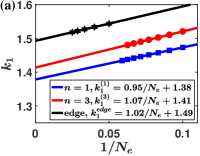
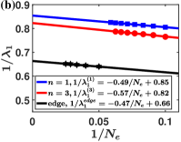
Figure S1: (a) Finite-size scaling of the wave vector $k_{1}$ for the single Laughlin quasihole (blue squares), $3$-Laughlin quasiholes (red circles), and the Laughlin edge (black hexagrams) at $\nu{=}1/3$. The lines are linear fits as a function of $1/N_{e}$. (b) Finite-size scaling of the inverse of the decay length $1/\lambda_{1}$.

SIII 1/3 Laughlin edge

We create a Laughlin edge by placing the Laughlin state on the disk geometry. Since the edge density fluctuation is large, we need a large system size (beyond the ones accessible to exact diagonalization) to reliably study it. Therefore, we determine the edge density using the Monte Carlo method. Then, we obtain the parameters of the damped model by fitting them to the real-space density. As shown in Fig. S2, the real-space density profile of the Laughlin edge can also be well-represented with the damped model in the occupation-number space. The parameters for different sizes are shown in Table  S3 and the finite size scaling is shown in Fig. S1.

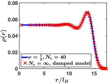
Figure S2: The density distribution of $1/3$ Laughlin state for $N_{e}=40$ in the disk (blue line). The red crosses denote the fitting using our damped model.

SIV 1/5 Laughlin state pair-correlation function

We also study the ground state pair-correlation function for $\nu{=}1/5$ Laughlin state using the Monte Carlo method and determine the parameters of the damped model by fitting the model to the real-space profile. As shown in Fig. S3, the pair-correlation function for the 1/5 Laughlin state can also be well-represented by our damped model. The parameters for different sizes and their thermodynamic extrapolation are shown in Table  S4. Then, we use the modeled $g(r)$ to calculate the per-particle variational energy of the Laughlin state in terms of the Coulomb interaction $V(r){=}1/r$, and the result is ${-}0.3278$, which is very close to the extrapolated result ${-}0.3275(1)$ obtained from exact diagonalization [35].

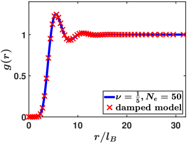
Figure S3: The ground state pair-correlation function for the $1/5$ Laughlin state for $N_{e}{=}50$ electrons in the spherical geometry (blue line). The red crosses denote the results obtained using our damped model.

SV General cases

By using the Jack polynomial method or Monte Carlo method, we can determine the occupation-number density or real-space density of Laughlin quasihole for various $m$ and $n$. Then, we can determine their characteristic lengths as done above and the results are summarized in Fig. 3. Based on the numerical results for various Laughlin quasiholes, we find the damped oscillation model can always reasonably capture the density-distribution of quasiholes, but its numerical accuracy ($R^{2}$ value) decreases increasing $m$ and $n$. The numerical accuracy dependence on $n$ can be seen by comparing the $R^{2}$ value of Table  S1 for $n{=}1$ and Table  S2 for $n{=}3$. The numerical accuracy dependence on $m$ can be seen by comparing the fitting in Fig. 2 for $m{=}3$ and Fig. S4 for $m{=}10$. For large values of $m$ and $n$, there are stronger finite-size effects which can potentially explain the lower numerical accuracy of the damped model. For these large values of $m$ and $n$, it is also possible that our model is unable to capture the physical features of the states accurately. When the density fluctuation is very strong, especially for large $m$, it is better to determine the characteristic lengths of the oscillation tail by starting from a finite $r$, e.g., the first zero point of $\delta\rho(r){=}0$.

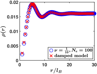
Figure S4: The real-space density of the single Laughlin quasihole at $\nu{=}1/10$ and $N_{e}{=}100$ electrons on the sphere (blue circles). The red crosses denote the results obtained using our damped model.

SVI Coulomb quasihole

In addition to the single-mode model of the Laughlin quasihole, another mode with four more fitting parameters is introduced for the Coulomb quasihole. The fitting parameters are shown in Table  S5. Note that numerical results show that there exist multiple sets of parameters that fit the density distribution very well. Therefore, it is possible that overfitting could be an issue for this model. We also find strong finite-size-scaling effects that hinder an accurate extrapolation to the thermodynamic limit.

$N_{e}$	$A_{1}$	$k_{1}$	$k_{1}*x_{1}$	$1/\lambda_{1}$	$A_{2}$	$k_{2}$	$k_{2}*x_{2}$	$1/\lambda_{2}$	$R^{2}$
10	0.2039	1.4965	2.7515	0.3778	0.5390	0.6411	2.0603	0.9143	0.999694
11	0.2283	1.4794	2.7356	0.4078	0.4948	0.6186	2.0792	0.8994	0.999920
12	0.2317	1.5039	2.8840	0.4202	0.5449	0.4572	1.5763	0.9318	0.999933
13	0.2232	1.4982	2.8624	0.4129	0.5375	0.5095	1.7350	0.9445	0.999845
14	0.2262	1.4847	2.8172	0.4160	0.5115	0.5425	1.8643	0.9318	0.999861

Table S5: Parameters of the double-damped model for the Coulomb quasihole with $N_{e}$ electrons at $\nu{=}1/3$.

$N_{e}$	$A_{1}$	$k_{1}$	$k_{1}*x_{1}$	$1/\lambda_{1}$	$A_{2}$	$k_{2}$	$k_{2}*x_{2}$	$1/\lambda_{2}$	$R^{2}$
15	0.9540	1.5628	5.7802	0.5936	7.3000	1.4715	3.4053	1.5951	0.999434
17	0.9761	1.5274	5.6332	0.6076	7.5191	1.4616	3.3479	1.6510	0.999540
19	1.0409	1.5138	5.5905	0.6273	6.9436	1.4817	3.3604	1.6286	0.999566
21	1.0593	1.5009	5.5481	0.6354	6.6887	1.4837	3.3545	1.6288	0.999598
$\infty$	1.3437	1.3457	4.9646	0.7451	5.0878	1.5220	3.2328	1.7069

Table S6: Parameters of the double-damped model for the Moore-Read quasihole density proportional to the ground state pair-correlation function. The last row is the thermodynamic extrapolation result as a function of $1/N_{e}$.

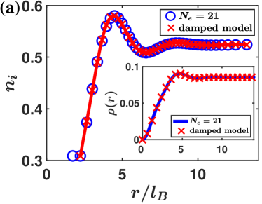
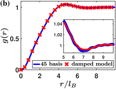
Figure S5: (a) The occupation numbers of the Moore-Read quasihole, the density of which is proportional to the Moore-Read ground state pair-correlation function, for $N_{e}{=}21$ electrons in the spherical geometry. Blue circles (red crosses) denote the exact (fitted) density. The inset is the corresponding real-space density. (b) The Moore-Read ground state pair-correlation function in the thermodynamic limit. The blue line and red crosses denote the results derived using the polynomial expansion method with $45$ basis [29] and our double-damped model, respectively. The inset is the zoomed view of the oscillation tail.

SVII pair-correlation function of Moore-Read state

The double-damped oscillation model also gives a good representation of the densities of Abelian quasiholes obtained from flux insertion (but no further fractionalization) for many other kinds of model FQH states. As an example, we show how to model the pair-correlation function of the Moore-Read ground state in the thermodynamic limit from it. To reduce the finite-size-scaling effects, we first determine the parameters of the long-range mode by fitting with the occupation numbers at a large $r$ (here our fitting starts from $n_{8}$), and then we determine the parameters of the short-range mode using all occupation numbers except the first two special orbitals. In this way, the finite-size effect is greatly reduced and meanwhile, the accuracy is still good as shown in Table  S6 and Fig. S5(a). The result obtained from an extrapolation to the thermodynamic limit is shown in Fig. S5(b). For comparison, we also plot the corresponding result obtained from the polynomial expansion method [29]. The two methods produce very similar results with a root-mean-square difference of $2{\times}10^{-3}$). Nevertheless, the density profile obtained from our model is smoother than that obtained using the polynomial expansion method.

References

- Giuliani and Vignale [2008] G. Giuliani and G. Vignale, Quantum theory of the electron liquid (Cambridge university press, 2008).
- Haldane [1981] F. Haldane, ’luttinger liquid theory’of one-dimensional quantum fluids. i. properties of the luttinger model and their extension to the general 1d interacting spinless fermi gas, Journal of Physics C: Solid State Physics 14, 2585 (1981).
- Halperin et al. [1993] B. I. Halperin, P. A. Lee, and N. Read, Theory of the half-filled Landau level, Phys. Rev. B 47, 7312 (1993).
- Klitzing et al. [1980] K. v. Klitzing, G. Dorda, and M. Pepper, New Method for High-Accuracy Determination of the Fine-Structure Constant Based on Quantized Hall Resistance, Phys. Rev. Lett. 45, 494 (1980).
- Tsui et al. [1982] D. C. Tsui, H. L. Stormer, and A. C. Gossard, Two-Dimensional Magnetotransport in the Extreme Quantum Limit, Phys. Rev. Lett. 48, 1559 (1982).
- Anderson [2006] P. W. Anderson, The ‘strange metal’ is a projected Fermi liquid with edge singularities, Nature Phys 2, 626 (2006).
- Senaratne et al. [2022] R. Senaratne, D. Cavazos-Cavazos, S. Wang, F. He, Y.-T. Chang, A. Kafle, H. Pu, X.-W. Guan, and R. G. Hulet, Spin-charge separation in a one-dimensional Fermi gas with tunable interactions, Science 376, 1305 (2022).
- Halperin [2020] B. I. Halperin, The half-full landau level, in Fractional quantum Hall effects: New developments (World Scientific, 2020) pp. 79–132.
- Kamilla et al. [1997] R. K. Kamilla, J. K. Jain, and S. M. Girvin, Fermi-sea-like correlations in a partially filled Landau level, Phys. Rev. B 56, 12411 (1997).
- Chang [2003] A. M. Chang, Chiral Luttinger liquids at the fractional quantum Hall edge, Rev. Mod. Phys. 75, 1449 (2003).
- Balram et al. [2015] A. C. Balram, C. Tőke, and J. Jain, Luttinger Theorem for the Strongly Correlated Fermi Liquid of Composite Fermions, Phys. Rev. Lett. 115, 186805 (2015).
- Balram and Jain [2017] A. C. Balram and J. K. Jain, Fermi wave vector for the partially spin-polarized composite-fermion Fermi sea, Phys. Rev. B 96, 235102 (2017).
- Mitrano et al. [2018] M. Mitrano, A. Husain, S. Vig, A. Kogar, M. Rak, S. Rubeck, J. Schmalian, B. Uchoa, J. Schneeloch, R. Zhong, et al., Anomalous density fluctuations in a strange metal, Proceedings of the National Academy of Sciences 115, 5392 (2018).
- Laughlin [1983] R. B. Laughlin, Anomalous Quantum Hall Effect: An Incompressible Quantum Fluid with Fractionally Charged Excitations, Phys. Rev. Lett. 50, 1395 (1983).
- Arovas et al. [1984] D. Arovas, J. R. Schrieffer, and F. Wilczek, Fractional Statistics and the Quantum Hall Effect, Phys. Rev. Lett. 53, 722 (1984).
- Trung et al. [2023] H. Q. Trung, Y. Wang, and B. Yang, Spin-statistics relation and Abelian braiding phase for anyons in the fractional quantum Hall effect, Phys. Rev. B 107, L201301 (2023).
- Park and Haldane [2014] Y. Park and F. D. M. Haldane, Guiding-center Hall viscosity and intrinsic dipole moment along edges of incompressible fractional quantum Hall fluids, Phys. Rev. B 90, 045123 (2014).
- Datta et al. [1996] N. Datta, R. Morf, and R. Ferrari, Edge of the Laughlin droplet, Phys. Rev. B 53, 10906 (1996).
- Wen [1990] X. G. Wen, Chiral Luttinger liquid and the edge excitations in the fractional quantum Hall states, Phys. Rev. B 41, 12838 (1990).
- Levesque et al. [2000] D. Levesque, J.-J. Weis, and J. Lebowitz, Charge fluctuations in the two-dimensional one-component plasma, Journal of Statistical Physics 100, 209 (2000).
- Wiegmann [2012] P. Wiegmann, Nonlinear Hydrodynamics and Fractionally Quantized Solitons at the Fractional Quantum Hall Edge, Phys. Rev. Lett. 108, 206810 (2012).
- Can et al. [2014] T. Can, P. J. Forrester, G. Téllez, and P. Wiegmann, Singular behavior at the edge of Laughlin states, Phys. Rev. B 89, 235137 (2014).
- Fern and Simon [2017] R. Fern and S. H. Simon, Quantum Hall edges with hard confinement: Exact solution beyond Luttinger liquid, Phys. Rev. B 95, 201108 (2017).
- Ito and Shibata [2021] T. Ito and N. Shibata, Density matrix renormalization group study of the edge states in fractional quantum Hall systems, Phys. Rev. B 103, 115107 (2021).
- Cardoso et al. [2021] G. Cardoso, J.-M. Stéphan, and A. G. Abanov, The boundary density profile of a Coulomb droplet. Freezing at the edge, J. Phys. A: Math. Theor. 54, 015002 (2021).
- Yang and Hu [2023] Y. Yang and Z.-X. Hu, Monte Carlo simulation of the topological quantities in fractional quantum Hall systems, Phys. Rev. B 107, 115162 (2023).
- Girvin et al. [1986] S. M. Girvin, A. H. MacDonald, and P. M. Platzman, Magneto-roton theory of collective excitations in the fractional quantum Hall effect, Phys. Rev. B 33, 2481 (1986).
- Johri et al. [2014] S. Johri, Z. Papić, R. N. Bhatt, and P. Schmitteckert, Quasiholes of 1 3 and 7 3 quantum Hall states: Size estimates via exact diagonalization and density-matrix renormalization group, Phys. Rev. B 89, 115124 (2014).
- Fulsebakke et al. [2023] J. Fulsebakke, M. Fremling, N. Moran, and J. K. Slingerland, Parametrization and thermodynamic scaling of pair correlation functions for the fractional quantum Hall effect, SciPost Phys. 14, 149 (2023).
- Haldane [1983] F. D. M. Haldane, Fractional Quantization of the Hall Effect: A Hierarchy of Incompressible Quantum Fluid States, Phys. Rev. Lett. 51, 605 (1983).
- [31] See Supplemental Material (SM) for detailed numerical data of fitting parameters and related analysis. The SM includes Ref. [50]. .
- Jain [2007] J. Jain, Composite Fermions (Cambridge University Press, 2007).
- Ciftja and Wexler [2003] O. Ciftja and C. Wexler, Monte Carlo simulation method for Laughlin-like states in a disk geometry, Phys. Rev. B 67, 075304 (2003).
- Balram and Wójs [2020] A. C. Balram and A. Wójs, Fractional quantum Hall effect at , Phys. Rev. Res. 2, 032035 (2020).
- Dora and Balram [2023] R. K. Dora and A. C. Balram, Competition between fractional quantum Hall liquid and electron solid phases in the Landau levels of multilayer graphene, Phys. Rev. B 108, 235153 (2023).
- Wigner [1934] E. Wigner, On the interaction of electrons in metals., Phys. Rev. 46, 1002 (1934).
- Balram et al. [2013a] A. C. Balram, Y.-H. Wu, G. J. Sreejith, A. Wójs, and J. K. Jain, Role of Exciton Screening in the 7 / 3 Fractional Quantum Hall Effect, Phys. Rev. Lett. 110, 186801 (2013a).
- Balram et al. [2013b] A. C. Balram, A. Wójs, and J. K. Jain, State counting for excited bands of the fractional quantum Hall effect: Exclusion rules for bound excitons, Phys. Rev. B 88, 205312 (2013b).
- Yang et al. [2012] B. Yang, Z.-X. Hu, Z. Papić, and F. D. M. Haldane, Model Wave Functions for the Collective Modes and the Magnetoroton Theory of the Fractional Quantum Hall Effect, Phys. Rev. Lett. 108, 256807 (2012).
- Mandal and Jain [2001] S. S. Mandal and J. Jain, How universal is the fractional-quantum-hall edge luttinger liquid?, Solid state communications 118, 503 (2001).
- Wan et al. [2005] X. Wan, F. Evers, and E. H. Rezayi, Universality of the Edge-Tunneling Exponent of Fractional Quantum Hall Liquids, Phys. Rev. Lett. 94, 166804 (2005).
- Yang [2021] B. Yang, Statistical Interactions and Boson-Anyon Duality in Fractional Quantum Hall Fluids, Phys. Rev. Lett. 127, 126406 (2021).
- Moore and Read [1991] G. Moore and N. Read, Nonabelions in the fractional quantum hall effect, Nuclear Physics B 360, 362 (1991).
- Read and Green [2000] N. Read and D. Green, Paired states of fermions in two dimensions with breaking of parity and time-reversal symmetries and the fractional quantum Hall effect, Phys. Rev. B 61, 10267 (2000).
- Simon et al. [2007] S. H. Simon, E. H. Rezayi, N. R. Cooper, and I. Berdnikov, Construction of a paired wave function for spinless electrons at filling fraction , Phys. Rev. B 75, 075317 (2007).
- Read and Rezayi [1999] N. Read and E. Rezayi, Beyond paired quantum Hall states: Parafermions and incompressible states in the first excited Landau level, Phys. Rev. B 59, 8084 (1999).
- Jain [1989] J. K. Jain, Composite-fermion approach for the fractional quantum Hall effect, Phys. Rev. Lett. 63, 199 (1989).
- Zhao et al. [2011] J. Zhao, D. N. Sheng, and F. D. M. Haldane, Fractional quantum Hall states at 1 3 and 5 2 filling: Density-matrix renormalization group calculations, Phys. Rev. B 83, 195135 (2011).
- [49] DiagHam, https://www.nick-ux.org/diagham.
- Bernevig and Haldane [2008] B. A. Bernevig and F. D. M. Haldane, Model Fractional Quantum Hall States and Jack Polynomials, Phys. Rev. Lett. 100, 246802 (2008).