Gravitational waves and orbital evolution for eccentric compact binaries in scalar-tensor theories at second post-Newtonian order

Abstract

The generalized post-Keplerian parametrization for compact binaries on eccentric bound orbits is established at second post-Newtonian (2PN) order in a class of massless scalar-tensor theories. This result is used to compute the orbit-averaged flux of energy and angular momentum at Newtonian order, which means relative 1PN order beyond the leading-order dipolar radiation of scalar-tensor theories. The secular evolution of the orbital elements is then computed at 1PN order. At leading order, the closed form “Peters & Matthews” relation between the semi-major axis $a$ and the eccentricity $e$ is found to be independent of any scalar-tensor parameter, and is given by $a\propto e^{4/3}/(1-e^{2})$. Finally, the waveform is obtained at Newtonian order in the form of a spherical harmonic mode decomposition, extending to eccentric orbits the results obtained in [JCAP 08 (2022) 008].

I Introduction

The LIGO-Virgo-KAGRA collaboration has so far detected more than 90 gravitational wave (GW) events [2], and future ground-based and spaceborne GW detectors such as LISA, Einstein Telescope and Cosmic Explorer open new horizons for the observation of the Universe. So far, all events are compatible with general relativity (GR), but current detectors only probe a small subset of binary systems, namely stellar-mass binaries near merger. Moreover, since events are detected by matched filtering under the premise that the waveform should be described by GR, it is not excluded that a subpopulation of gravitational wave events exhibiting large deviations from GR have been missed in the data due to selection biases [3]. One approach to modeling alternative theories is to take a theory-agnostic, parametrized approach [4, 5, 6, 7]. In this paper, I instead opt for a theory-dependent approach, and derive predictions for the gravitational waveform within the class of massless scalar-tensor (ST) theories of gravity, which were first introduced by Jordan [8], Fierz [9] and Brans & Dicke [10], and later generalized in [11, 12]. Binary pulsar observations have already put strong constraints on the parameters entering the models [13, 14, 15, 16, 17], but nonperturbative phenomena appearing in the later stages of the inspiral could potentially help evade these constraints, such as dynamical scalarizatio [18, 19]. Due to the no-hair theorem in ST theory, valid for stationary isolated black holes [20, 21], one expects that the motion and radiation of binary black holes (BHs) are indistinguishable from those of the GR solution. To some extent, this expectation has been confirmed by numerical relativity calculations [22]. Consequently, relevant theory-dependent tests for ST theory involve binary neutron stars (or more exotic extended compact objects) as well as asymmetrical black hole-neutron star (BH-NS) binaries [23, 24, 25].

I will work within the post-Newtonian (PN) formalism, i.e. an approximation for weak gravitational fields and small orbital velocities, and I will consequently focus on the inspiraling phase of coalescing binary systems. Previous results in massless ST theories using the PN expansion were derived using i) effective field theory methods [13, 26, 27, 28, 29]; ii) the Direct Integration of the Relaxed field Equations (DIRE) method [30, 31, 32, 33, 34]; and iii) the post-Newtonian, multipolar post-Minkowskian (PN-MPM) scheme [35, 36, 1, 37, 38]. It is the latter scheme that I will use hereafter, as it has been successfully used in GR to compute the energy flux and GW phasing at very high fourth-and-a-half post-Newtonian (4.5PN) order [39, 40, 41, 42, 43, 44, 45, 46, 47, 48].

Gravitational radiation in ST theories was first studied by [13, 26, 49, 28, 29] in an alternative (but equivalent) formulation of the action. The equations of motion and conserved energy and angular momentum were first obtained at 2.5PN order in [32], then at 3PN order in [35, 36], including the contribution of the (dipolar) tail term. The waveform and flux was first obtained in the tensor sector at 2PN [33] and in the scalar sector at 1PN [34] beyond quadrupolar radiation (i.e. relative 2PN order beyond the leading-order scalar dipolar radiation). The flux was then reduced to circular orbits at 2PN in tensor sector and 1PN in the scalar sector [50]. The phase at 1PN and the tensor spherical harmonic modes at 2PN were computed as well [50]. Finally, the complete (tensor and scalar) flux for generic orbits was computed at 1.5PN in [1], along with its reduction to circular orbits. Moreover, the scalar and tensor spherical harmonic modes were computed for circular orbits at 1PN order, and the phase at 1.5PN order [1]. The equations of motion and gravitational radiation has also been studied in extensions to massless scalar-tensor theories, e.g. massive ST theory [51], massless multiscalar-tensor theory [52], Einstein-Æther theory [53], scalar-Gauss-Bonnet theory [54], Horndeski theory [55, 56], etc.

In GR, gravitational waves generated by eccentric binaries were first studied at Newtonian order in the seminal work of Peters and Mattews [57, 58]. An elegant generalization of the Kepler solution to first post-Newtonian (1PN) order, dubbed the post-Keplerian (PK) parametrization, was then introduced by Damour and Deruelle [59]. This parametrization was then generalized for spinless systems at 2PN [60, 61], 3PN [62] and finally 4PN order [63], including a semi-analytical treatment of the tail term (although certain zero-average, oscillatory terms are ignored). The gravitational waveform and energy flux were first computed at 1PN order in [64, 65] and the 1PN angular momentum flux, waveform and secular evolution of the orbital parameters were computed in [66]. The hereditary tail effects entering at 1.5PN were first dealt with in the case of eccentric orbtis in [67, 68]. At 2PN order, the energy and angular momentum fluxes, the secular evolution of the orbital elements and the waveform were computed by [69]. At 3PN, these same quantities were computed in the series of works [70, 71, 72], which also treat higher-order tails and the memory integral which enters the angular momentum flux at this order. Moreover, the amplitudes of the spherical harmonic modes were computed in [73, 74, 75]. Partial results at 4PN for the waveform and orbital element evolution are given in [63].

Fewer results have been derived for eccentric systems in the context of ST theories. The parametrized post-Keplerian (PKK) parametrization was introduced in [76], and applied at leading order to obtain some predictions for tensor-multiscalar theories [49]. In the case of monoscalar-tensor theories, the effects have been briefly studied in [77], as well as in [78, 79]. In the case of ST theories with screening generated by a potential, eccentric orbits have been investigated more in detail in [80].

This work is a direct continuation of Ref. [1], hereafter Paper I, and aims at systematically extending the results for circular orbits therein to the case of an eccentric orbit with the help of the PK parametrization. The system is assumed to be dipole-driven, and the quadrupole-driven case is left for further investigation (see [50] for a discussion). After a brief notational subsection, the main features of the ST theories under consideration are introduced in Sec. II, as well as the multipolar post-Minkowskian (MPM) construction. Sec. III is devoted to the derivation of the post-Keplerian parametrization at 2PN order (denoted 2PK) in the context of alternative theories of gravity. Generic results are first derived in a class of alternative theories that I will define precisely. Then, these results are specialized to the case of ST theories. The reason for this split is to provide generic expressions that will, in the future, facilitate the computation of the PK parametrization for other theories of gravity. In Sec. IV, the orbit-averaged fluxes of energy and angular momentum are computed at Newtonian order, which corresponds to the next-to-leading order beyond the dominant dipolar radiation. Sec. V is devoted to the computation of the evolution of the orbital elements. I first focus on the $-1$PN, leading order terms, for which there is no ambiguity in the definition of the semi-major axis $a$ and eccentricity $e$. In this case, I find closed form expressions akin to those of Peters and Matthews [57, 58], such as $a\propto e^{4/3}/(1-e^{2})$, and compare the orbital decay between ST theory and GR in the leading-order case. Then, I compute the 1PN expression of the two ordinary differential equations (ODEs) describing the time evolution of the pair of variables $(x,e_{t})$. Since all other orbital parameters are explicitly given in this paper in terms of this pair of variables, their time evolution is straightforward to obtain. Finally, Sec. VI describes the waveform at (next-to-leading) Newtonian order as a mode decomposition over spherical harmonics, which is a useful result for numerical relativists.

Main notations and summary of parameters

The convention in this work is that all stated PN orders are, by default, relative to the the Newtonian dynamics and the standard quadrupole radiation in GR. Thus, the dominant dipole radiation enters at $-0.5$PN order in the waveform and at $-1$PN order in the energy flux. The 2PK parametrization computed in the paper is therefore next-to-next-to-leading-order, while the Newtonian fluxes and waveforms are next-to-leading order.

After a 3+1 decomposition of spacetime, and using the convention that boldface letters represent three-dimensional Euclidean vectors, the field-point spatial vector in the center-of-mass (CM) frame is denoted by $\bm{X}=R\,\bm{N}$, where $\bm{N}$ has unit norm. In spherical coordinates, the coordinates of the field point are denoted by $(R,\Theta,\Phi)$. Time is denoted by $t$, and retarded time is defined as $U=t-R/c$, so as to not confuse it with the eccentric anomaly of the PK motion, $u$. The usual spherical harmonics $Y^{\ell\mathrm{m}}(\Theta,\Phi)$ will be used, alongside the spin-weighted ones (with weight $-2$), $Y_{-2}^{\ell\mathrm{m}}(\Theta,\Phi)$, where the integer $\mathrm{m}$ should not be confused with the total mass $m$.

The positions of particles 1 and 2 are denoted by $\bm{y}_{1}$ and $\bm{y}_{2}$, and $\bm{x}=\bm{y}_{1}-\bm{y}_{2}$ is the separation vector. The orbital radius is given by $r=|\bm{x}|$, and the unit vector $\bm{n}=\bm{x}/r$ is introduced. The relative velocity is given by $\bm{v}=\differential\bm{x}/\differential t$. For a nonprecessing eccentric compact binary in the CM frame, one can then introduce the orthonormal triad $(\bm{n},\bm{\lambda},\bm{\ell})$ such that $\bm{\lambda}$ lies in the orbital plane, $\bm{\lambda}\cdot\bm{v}>0$ and $\bm{\ell}=\bm{n}\times\bm{\lambda}$. Introducing some reference, nonrotating reference triad $(\bm{n}_{0},\bm{\lambda}_{0},\bm{\ell})$, one can then describe the orbital motion by the polar coordinates $(r,\phi)$ such that $\bm{n}=\cos\phi\,\bm{n}_{0}+\sin\phi\,\bm{\lambda}_{0}$. Notice that the relative velocity is given by $\bm{v}=\dot{r}\bm{n}+r\dot{\phi}\bm{\lambda}$. The following relations then hold: $\bm{n}\cdot\bm{\lambda}=\dot{r}$, $v^{2}=\dot{r}^{2}+r^{2}\dot{\phi}r^{2}$ and $\bm{n}\times\bm{v}=r\dot{\phi}\bm{\ell}$.

The notation $L=i_{1}\cdots i_{\ell}$ stands for multi-index with $\ell$ spatial indices (and $K$ would stand for a multi-index with $k$ spatial indices). One can then write $\partial_{L}=\partial_{i_{1}}\cdots\partial_{i_{\ell}}$, $\partial_{aL-1}=\partial_{a}\partial_{i_{1}}\cdots\partial_{i_{\ell-1}}$ and so on; similarly, $n_{L}=n_{i_{1}}\cdots n_{i_{\ell}}$, $n_{aL-1}=n_{a}n_{i_{1}}\cdots n_{i_{\ell-1}}$. The symmetric trace-free (STF) part is indicated using a hat or angled brackets: for instance, $\mathrm{STF}_{L}[\partial_{L}]=\hat{\partial}_{L}=\partial_{\langle i_{1}}\partial_{i_{2}}\cdots\partial_{i_{\ell}\rangle}$, $\mathrm{STF}_{L}[n_{L}]=\hat{n}_{L}=n_{\langle i_{1}}n_{i_{2}}\cdots n_{i_{\ell}\rangle}$ and $\mathrm{STF}_{L}[x_{L}]=\hat{x}_{L}=r^{\ell}n_{\langle i_{1}}n_{i_{2}}\cdots n_{i_{\ell}\rangle}$. The $n$-th time derivative of a function $F(t)$ is denoted $F^{(n)}(t)=\differential^{n}F/\differential t^{n}$.

The constant asymptotic value of the scalar field at spatial infinity is denoted $\phi_{0}$, and the normalized scalar field is defined by $\varphi\equiv\phi/\phi_{0}$. The Brans-Dicke-like scalar function $\omega(\phi)$ is expanded around the asymptotic value $\omega_{0}\equiv\omega(\phi_{0})$ and the mass-functions $m_{A}(\phi)$ (see Section II for a definition) are expanded around the asymptotic values $m_{A}\equiv m_{A}(\phi_{0})$, where $A\in\{1,2\}$. In the CM frame, one then defines the asymptotic total mass $m=m_{1}+m_{2}$, reduced mass $\mu=m_{1}m_{2}/m$, symmetric mass ratio $\nu=\mu/m\in\ ]0,1/4]$ and relative mass difference $\delta=(m_{1}-m_{2})/m\in\ [0,1[$. Note that the asymptotic symmetric mass ratio and the relative mass difference are linked by the relation $\delta^{2}=1-4\nu$.

Following [35, 1], a number of parameters describing these expansions are introduced in Table 1. The ST parameters are defined directly from the expansions of the Brans-Dicke-like scalar function $\omega(\phi)$ and of the mass-functions $m_{A}(\phi)$. The PN parameters are combinations of the ST parameters that naturally extend and generalize the usual PPN parameters to the case of a general ST theory [81, 4].

	ST parameters
general	$\omega_{0}=\omega(\phi_{0}),\qquad\omega_{0}^{\prime}=\evaluated{\frac{\differential\omega}{\differential\phi}}_{\phi=\phi_{0}},\qquad\omega_{0}^{\prime\prime}=\evaluated{\frac{\differential^{2}\omega}{\differential\phi^{2}}}_{\phi=\phi_{0}},\qquad\varphi=\frac{\phi}{\phi_{0}},\qquad\tilde{g}_{\mu\nu}=\varphi\,g_{\mu\nu},$
	$\tilde{G}=\frac{G(4+2\omega_{0})}{\phi_{0}(3+2\omega_{0})},\qquad\zeta=\frac{1}{4+2\omega_{0}},$
	$\lambda_{1}=\frac{\zeta^{2}}{(1-\zeta)}\left.\frac{\differential\omega}{\differential\varphi}\right|_{\varphi=1},\qquad\lambda_{2}=\frac{\zeta^{3}}{(1-\zeta)}\left.\frac{\differential^{2}\omega}{\differential\varphi^{2}}\right|_{\varphi=1},\qquad\lambda_{3}=\frac{\zeta^{4}}{(1-\zeta)}\left.\frac{\differential^{3}\omega}{\differential\varphi^{3}}\right|_{\varphi=1}.$
sensitivities	$s_{A}=\evaluated{\frac{\differential\ln{m_{A}(\phi)}}{\differential\ln{\phi}}}_{\phi=\phi_{0}},\qquad s_{A}^{(k)}=\evaluated{\frac{\differential^{k+1}\ln{m_{A}(\phi)}}{\differential(\ln{\phi})^{k+1}}}_{\phi=\phi_{0}},\qquad(A=1,2)$
	$s^{\prime}_{A}=s_{A}^{(1)},\qquad s^{\prime\prime}_{A}=s_{A}^{(2)},\qquad s^{\prime\prime\prime}_{A}=s_{A}^{(3)},$
	$\mathcal{S}_{+}=\frac{1-s_{1}-s_{2}}{\sqrt{\alpha}}\,,\qquad\mathcal{S}_{-}=\frac{s_{2}-s_{1}}{\sqrt{\alpha}}.$
Order	PN parameters
N	$\alpha=1-\zeta+\zeta\left(1-2s_{1}\right)\left(1-2s_{2}\right)$
1PN	$\overline{\gamma}=-\frac{2\zeta}{\alpha}\left(1-2s_{1}\right)\left(1-2s_{2}\right),$	Degeneracy
	$\overline{\beta}_{1}=\frac{\zeta}{\alpha^{2}}\left(1-2s_{2}\right)^{2}\left(\lambda_{1}\left(1-2s_{1}\right)+2\zeta s^{\prime}_{1}\right),$	$\alpha(2+\overline{\gamma})=2(1-\zeta)$
	$\overline{\beta}_{2}=\frac{\zeta}{\alpha^{2}}\left(1-2s_{1}\right)^{2}\left(\lambda_{1}\left(1-2s_{2}\right)+2\zeta s^{\prime}_{2}\right),$
	$\overline{\beta}_{+}=\frac{\overline{\beta}_{1}+\overline{\beta}_{2}}{2},\qquad\overline{\beta}_{-}=\frac{\overline{\beta}_{1}-\overline{\beta}_{2}}{2}.$
2PN	$\overline{\delta}_{1}=\frac{\zeta\left(1-\zeta\right)}{\alpha^{2}}\left(1-2s_{1}\right)^{2}\,,\qquad\overline{\delta}_{2}=\frac{\zeta\left(1-\zeta\right)}{\alpha^{2}}\left(1-2s_{2}\right)^{2},$	Degeneracy
	$\overline{\delta}_{+}=\frac{\overline{\delta}_{1}+\overline{\delta}_{2}}{2},\qquad\overline{\delta}_{-}=\frac{\overline{\delta}_{1}-\overline{\delta}_{2}}{2},$	$16\overline{\delta}_{1}\overline{\delta}_{2}=\overline{\gamma}^{2}(2+\overline{\gamma})^{2}$
	$~{}~{}\overline{\chi}_{1}=\frac{\zeta}{\alpha^{3}}\left(1-2s_{2}\right)^{3}\left[\left(\lambda_{2}-4\lambda_{1}^{2}+\zeta\lambda_{1}\right)\left(1-2s_{1}\right)-6\zeta\lambda_{1}s^{\prime}_{1}+2\zeta^{2}s^{\prime\prime}_{1}\right],~{}~{}$
	$\overline{\chi}_{2}=\frac{\zeta}{\alpha^{3}}\left(1-2s_{1}\right)^{3}\left[\left(\lambda_{2}-4\lambda_{1}^{2}+\zeta\lambda_{1}\right)\left(1-2s_{2}\right)-6\zeta\lambda_{1}s^{\prime}_{2}+2\zeta^{2}s^{\prime\prime}_{2}\right],$
	$\overline{\chi}_{+}=\frac{\overline{\chi}_{1}+\overline{\chi}_{2}}{2},\qquad\overline{\chi}_{-}=\frac{\overline{\chi}_{1}-\overline{\chi}_{2}}{2}.$

Table 1: Summary of parameters for the general ST theory and notations for PN parameters.

II Massless scalar-tensor theories

As in Paper I, consider a generic class of ST theories in which a single massless scalar field $\phi$ minimally couples to the metric $g_{\mu\nu}$. It is described by the action

$$S_{\mathrm{ST}} =\frac{c^{3}}{16\pi G}\int\differential^{4}x\,\sqrt{-g}\left[\phi R-\frac{\omega(\phi)}{\phi}g^{\alpha\beta}\partial_{\alpha}\phi\partial_{\beta}\phi\right]$$

$$\qquad\quad+S_{\mathrm{m}}\left(\mathfrak{m},g_{\alpha\beta}\right)\,,$$ (1)

where $R$ and $g$ are respectively the Ricci scalar and the determinant of the metric, $\omega$ is a function of the scalar field and $\mathfrak{m}$ stands generically for the matter fields. The action for the matter $S_{\mathrm{m}}$ is a function only of the matter fields and the metric. A major difference in ST theories compared to GR is that, as a consequence of the breaking of the strong equivalence principle, one has to take into account the internal gravity of each body. Indeed, the scalar field determines the effective gravitational constant, which in turn affects the competition between gravitational and non-gravitational forces within the body. Thus, the value of the scalar field has an indirect influence on the size of the compact body and on its internal gravity. Here, I follow the approach pioneered by Eardley [82] (see also [83]) and take for $S_{\mathrm{m}}$ the effective action for $N$ non-spinning point-particles with the masses $m_{A}(\phi)$ depending in an unspecified manner on the value of the scalar field at the location of the particles, i.e.

$$S_{\mathrm{m}}=-c\sum_{A}\int\,m_{A}(\phi)\sqrt{-\left(g_{\alpha\beta}\right)_{A}\differential y_{A}^{\alpha}\,\differential y_{A}^{\beta}}\,,$$ (2)

where $y_{A}^{\alpha}$ denote the space-time positions of the particles, and $\left(g_{\alpha\beta}\right)_{A}$ is the metric evaluated at the position of particle $A$. Thus, the matter action depends indirectly on the scalar field, and the sensitivities of the particles to variations in the scalar field are defined by

$$s_{A}^{(k)}\equiv\evaluated{\frac{\differential^{k+1}\ln{m_{A}(\phi)}}{\differential(\ln{\phi})^{k+1}}}_{\phi=\phi_{0}}\,,$$ (3)

where $s_{A}\equiv s_{A}^{(1)}$ and $\phi_{0}$ are the values of the scalar field at spatial infinity that is assumed to be constant in time, i.e. the cosmological evolution is neglected. For stationary black holes, since all information regarding the matter which formed the black hole has disappeared behind the horizon, the mass can depend only on the Planck scale, $m_{A}\propto M_{\text{Planck}}\propto G^{-1/2}\propto\phi^{1/2}$ hence $s^{\text{BH}}_{A}={1}/{2}$. The action (II) is usually called the Jordan-frame action, as the matter only couples to the Jordan or “physical” metric $g_{\alpha\beta}$. It is then very useful to introduce a rescaled scalar field and a conformally related metric,

$$\varphi\equiv\frac{\phi}{\phi_{0}}\qquad\mathrm{and}\qquad\tilde{g}_{\alpha\beta}\equiv\varphi\,g_{\alpha\beta}\,,$$ (4)

such that the physical and conformal metrics have the same asymptotic behavior at spatial infinity. Quantities expressed in terms of the pair $(\varphi,\tilde{g}_{\alpha\beta})$ are said to be in the “Einstein frame”. From these, one defines the scalar and metric perturbation variables $\psi\equiv\varphi-1$ and $h^{\mu\nu}\equiv\sqrt{-\tilde{g}}\tilde{g}^{\mu\nu}-\eta^{\mu\nu}$, where $\eta^{\mu\nu}~{}=~{}\text{diag}(-1,1,1,1)$ is the Minkowski metric. The field equations then read

$$\Box_{\eta}\,h^{\mu\nu}=\frac{16\pi G}{c^{4}}\tau^{\mu\nu}\,,$$ (5a)

$$\Box_{\eta}\,\psi=-\frac{8\pi G}{c^{4}}\tau_{s}\,,$$ (5b)

where $\Box_{\eta}$ denotes the ordinary flat space-time d’Alembertian operator, and where the source terms read

$$\tau^{\mu\nu}=\frac{\varphi}{\phi_{0}}(-g)T^{\mu\nu}+\frac{c^{4}}{16\pi G}\Lambda^{\mu\nu}[h,\psi]\,,$$ (6a)

$$\tau_{s}=-\frac{\varphi}{\phi_{0}(3+2\omega)}\sqrt{-g}\left(T-2\varphi\frac{\partial T}{\partial\varphi}\right)-\frac{c^{4}}{8\pi G}\Lambda_{s}[h,\psi]\,.$$ (6b)

Here $T^{\mu\nu}=2(-g)^{-1/2}\delta S_{\mathrm{m}}/\delta g_{\mu\nu}$ is the matter stress-energy tensor, $T\equiv g_{\mu\nu}T^{\mu\nu}$ is its trace and $\partial T/\partial\varphi$ is defined as the partial derivative of $T(g_{\mu\nu},\varphi)$ with respect to $\varphi$ holding $g_{\mu\nu}$ constant. Moreover, $\Lambda^{\mu\nu}$ and $\Lambda^{s}$ are given explicitly in (2.8) and (2.9) of Paper I as functionals of the $h^{\mu\nu}$ and $\psi$ that are at least quadratic in the fields.

The field equations of (5) are solved using the post-Newtonian multipolar post-Minkowskian (PN-MPM) construction [87, 88]. The reader is invited to refer to Paper I for a detailed description of this construction in the case of ST theories. For the purposes of this work, I will only need to use the expressions of the so-called source moments $\mathrm{I}_{L}$, $\mathrm{J}_{L}$ and $\mathrm{I}_{L}^{s}$, which are pure functions of retarded time $U$ that are STF in their indices and uniquely parametrize the linearized metric $h_{1}^{\mu\nu}$ and the linearized scalar field $\psi_{1}$. For example, the linearized scalar field reads explicitly :

$$\psi_{1}=-\frac{2}{c^{2}}\sum_{\ell=0}^{+\infty}\frac{(-)^{\ell}}{\ell!}\,\partial_{L}\!\left[\frac{\mathrm{I}_{L}^{s}(U)}{R}\right]\,.$$ (7)

A feature of ST theory is that the scalar monopole $\mathrm{I}^{s}$ is not constant but its time-variation will be a small PN effect, i.e. $\differential\mathrm{I}^{s}/\differential t=\mathcal{O}(c^{-2})$. This is why the leading-order radiation in dipolar, and not monopolar. It is thus practical to define

$$\mathrm{I}^{s}(U)=\frac{1}{\phi_{0}}\left[m^{s}+\frac{E^{s}(U)}{c^{2}}\right]\,,$$ (8a)

where

$$m^{s}=-\frac{1}{3+2\omega_{0}}\sum_{A}m_{A}(1-s_{A})$$ (8b)

is constant and $E^{s}(U)$ is the time-varying PN correction.

The gravitational and scalar waves, when viewed by an asymptotic observer [i.e. $Gm/(c^{2}R_{\mathrm{obs}})\ll 1$, where $R_{\mathrm{obs}}$ is the distance of the observer to the source], admits a multipolar decomposition as well. Introducing some radiative coordinates $(T,R,\bm{N})$ [or alternatively $(T,R,\Theta,\Phi)$], which ensure that the asymptotic structure of the waveform is parametrized by three families of radiative moments [88, 1], which are denoted $\mathcal{U}_{L}$, $\mathcal{V}_{L}$ and $\mathcal{U}^{s}_{L}$. It reads in a transverse-traceless gauge

$$h_{ij}^{\text{TT}} =-\frac{4G}{c^{2}R}\perp^{\text{TT}}_{ijab}\sum_{\ell=2}^{+\infty}\frac{1}{c^{\ell}\ell!}\Bigg{[}N_{L-2}\,\mathcal{U}_{abL-2}(U)$$

$$\qquad-\frac{2\ell}{c(\ell+1)}N_{cL-2}\epsilon_{cd(a}\mathcal{V}_{b)dL-2}(U)\Bigg{]}+\mathcal{O}\Big{(}\frac{1}{R^{2}}\Big{)}\,,$$ (9a)

$$\psi =-\frac{2G}{c^{2}R}\sum_{\ell=0}^{+\infty}\frac{1}{c^{\ell}\ell!}N_{L}\mathcal{U}_{L}^{s}(U)+\mathcal{O}\Big{(}\frac{1}{R^{2}}\Big{)}\,,$$ (9b)

where $\perp_{ijab}^{\mathrm{TT}}=\perp_{a(i}\perp_{j)b}-\frac{1}{2}\!\perp_{ij}\perp_{ab}$ with $\perp_{ij}=\delta_{ij}-N_{i}N_{j}$. The radiative moments are related to the source moments by the relations

$$\mathcal{U}_{L}(U) =\overset{(\ell)}{\mathrm{I}}_{\!\!L}(U)+\mathcal{O}\left(\frac{1}{c^{3}}\right)\,,$$ (10)

$$\mathcal{V}_{L}(U) =\overset{(\ell)}{\mathrm{J}}_{\!\!L}(U)+\mathcal{O}\left(\frac{1}{c^{3}}\right)\,,$$ (11)

$$\mathcal{U}^{s}_{L}(U) =\overset{(\ell)}{\mathrm{I}^{s}}_{\!\!L}(U)+\mathcal{O}\left(\frac{1}{c^{3}}\right)\,,$$ (12)

where the small $\mathcal{O}(1/c^{3})$ corrections correspond to the nonlinear corrections of the MPM construction, such as tails or memory integrals [see Paper I for details]. In this work, only the linear part of the MPM construction is needed.

III The post-Keplerian parametrization

III.1 General case

Consider the conservative dynamics of spinless binary system, characterized by the expression of the conserved energy $E$ and angular momentum $\bm{J}$ (whose norm is denoted $J=|\bm{J}|$) in terms of the relative position $\mathbf{r}$ and velocity $\mathbf{v}$ of the two objects. If the motion is planar, it in principle possible to invert these relation to obtain the dynamics in the following form:

$$\dot{r}^{2} =s^{-4}\dot{s}=\mathcal{R}(s,E,J)\,,$$ (13a)

$$\dot{\phi} =\mathcal{S}(s,E,J)\,,$$ (13b)

where $s\equiv 1/r$. In this section, I thus assume that we are working in a generic theory of gravity which can be studied perturbatively using the PN methodology and whose 2PN equations of motion in the CM frame can be cast in the form of (13), where $\mathcal{R}$ and $\mathcal{S}$ are fitfth-order polynomials in $s$ which have the following structure (see Sec. III.2 for how this structure arises in the particular case of ST theories):

$$\mathcal{R}(s,E,J) =A+Bs+Cs^{2}+D_{1}s^{3}+D_{2}s^{4}+D_{3}s^{5}\,,$$ (14a)

$$\mathcal{S}(s,E,J) =Fs^{2}+I_{1}s^{3}+I_{2}s^{4}+I_{3}s^{5}\,.$$ (14b)

Here, $A$, $B$, $C$ and $F$ are constants of order $\mathcal{O}(1)$, $D_{1}$ and $I_{1}$ are of order $\mathcal{O}(c^{-2})$ and $D_{2}$, $D_{3}$, $I_{2}$ and $I_{3}$ are of order $\mathcal{O}(c^{-4})$. In particular, note the absence of any logarithmic term (which would typically appear in standard harmonic coordinates at higher order) or nonlocal tail terms. In GR, the expressions of these coefficients are well known [59, 60, 61], while their expressions in massless ST theories will be computed in Sec. III.2. Thanks to the results given in (20) of this Section, it will suffice to obtain an equation of the form (14) for any given theory of gravity to automatically know the PK parametrization at 2PN order.

Dropping from now on the dependencies in $E$ and $J$, the previous assumptions imply that the polynomial $\mathcal{R}$ has exactly two roots that are nonzero in the $c\rightarrow\infty$ limit: denote these by $s_{p}=1/r_{p}$ and $s_{a}=1/r_{a}$, where “$p$” and “$a$” stand for periastron and apastron respectively (thus $r_{p}<r_{a}$ and $s_{p}>s_{a}$). One then obtains the factorization

$$\mathcal{R}(s)=(s-s_{p})(s-s_{a})\widetilde{\mathcal{R}}(s)\,,$$ (15)

where $\widetilde{\mathcal{R}}(s)$ is a third-order polynomial. One can iteratively compute these roots to desired 2PN precision.

In the PK motion, the orbital period $P$ is defined as the time of return to the periastron, which reads

$$P=2\int_{s_{a}}^{s_{p}}\frac{\differential s}{s^{2}\sqrt{\mathcal{R}(s)}}\,.$$ (16a)

From this it is useful to define the mean motion $$n=2\pi/P \ell=n(t-t_{0}) P \phi 2\pi P$$ and the mean anomaly . During one period , the true anomaly does not increase by , but by a bit more, due to the well known advance of the periastron. The increase in the true anomaly per period is given by

$$\Phi=2\int_{s_{a}}^{s_{p}}\frac{\differential s\,\mathcal{S}(s)}{s^{2}\sqrt{\mathcal{R}(s)}}\,.$$ (16b)

One defines from it the quantity $K=\Phi/(2\pi)$, as well as $k=K-1$ and $\Delta\Phi=2\pi k$.

These periods are most efficiently computed to some finite PN accuracy using complex analysis methods, which are described in App. A. The end result (given in machine-readable form in the Supplementary Material [89]) at 2PN accuracy reads

$$n =\frac{(-A)^{3/2}}{B}+\frac{A^{3}(12BD_{3}+3D_{1}^{2}-4CD_{2})}{8B^{2}(-C)^{5/2}}\,,$$ (17a)

$$K =\frac{F}{\sqrt{-C}}+\frac{B(3FD_{1}-2CI_{1})}{2(-C)^{5/2}}$$

$$\quad+\frac{1}{16(-C)^{9/2}}\Big{(}105B^{2}FD_{1}^{2}-15ACFD_{1}^{2}$$

$$\qquad-60B^{2}CFD_{2}+12AC^{2}FD_{2}+140B^{3}FD_{3}$$

$$\qquad-60ABCFD_{3}-60B^{2}CD_{1}I_{1}+12AC^{2}D_{1}I_{1}$$

$$\qquad+24B^{2}C^{2}I_{2}-8AC^{3}I_{2}-40B^{3}CI_{3}+24ABC^{2}I_{3}\Big{)}\,,$$ (17b)

and the expression for $n$ agrees at lowest order with (3.5a) of [59]. The PK parametrization is formally valid as soon as one can write down Eq. (14). At 2PN order, it reads [60, 61]

$$r =a_{r}(1-e_{r}\cos(u))\,,$$ (18a)

$$\ell=n(t-t_{0}) =u-e_{t}\sin(u)+f_{t}\sin(v)+g_{t}(v-u)\,,$$ (18b)

$$\frac{2\pi}{\Phi}(\phi-\phi_{0}) =v+f_{\phi}\sin(2v)+g_{\phi}\sin(3v)\,,$$ (18c)

where $u$ is called the eccentric anomaly, and

$$v=2\arctan\left[\sqrt{\frac{1+e_{\phi}}{1-e_{\phi}}}\tan\left(\frac{u}{2}\right)\right]\,.$$ (19)

The detailed construction of the different PK parameters is described in App. B. Here, let me simply highlight the following facts. First, $g_{t}$, $f_{t}$, $g_{\phi}$ and $f_{\phi}$ are all $\sim\mathcal{O}(c^{-4})$, and vanish at the 1PN level. Second, the three eccentricities $e_{r}$, $e_{\phi}$ and $e_{t}$ are equal at Newtonian level. Third, one has the straightforward relations $a_{r}=(s_{p}+s_{a})/(2s_{a}s_{p})$ and $e_{r}=(s_{p}-s_{a})/(s_{p}+s_{a})$.

The expressions for the values of the different PK parameters in terms of $A$, $B$, $C$, $D_{n}$, $F$ and $I_{n}$ are presented hereafter. The expressions in the case of the massless ST theories of (II) are given in App. C. Both results are provided in machine-readable form in the Supplementary Material [89].

$$a_{r} =-\frac{B}{A}+\frac{D_{1}}{2C}+\frac{2BD_{1}^{2}-2BCD_{2}+4B^{2}D_{3}-ACD_{3}}{2C^{3}}+\mathcal{O}\left(\frac{1}{c^{4}}\right)\,,$$ (20a)

$$e_{r} =\sqrt{1-\frac{AC}{B^{2}}}+\frac{AD_{1}(2B^{2}-AC)}{2B^{2}C\sqrt{B^{2}-AC}}$$

$$\quad+\frac{A}{8B^{3}C^{3}(B^{2}-AC)^{3/2}}\Big{(}16B^{6}D_{1}^{2}-24AB^{4}CD_{1}^{2}+5A^{2}B^{2}C^{2}D_{1}^{2}+2A^{3}C^{3}D_{1}^{2}-16B^{6}CD_{2}+28AB^{4}C^{2}D_{2}$$

$$\qquad\qquad\qquad\qquad\qquad\qquad-12A^{2}B^{2}C^{3}D_{2}+32B^{7}D_{3}-64AB^{5}CD_{3}+36A^{2}B^{3}C^{2}D_{3}-4A^{3}BC^{3}D_{3}\Big{)}+\mathcal{O}\left(\frac{1}{c^{4}}\right)\,,$$ (20b)

$$e_{t} =\sqrt{1-\frac{AC}{B^{2}}}+\frac{AD_{1}}{2C\sqrt{B^{2}-AC}}+\frac{(-A)^{3/2}\sqrt{B^{2}-AC}}{8B^{2}(-C)^{5/2}}\left(4CD_{2}-12BD_{3}-3D_{1}^{2}\right)$$

$$\qquad+\frac{A}{8BC^{3}(B^{2}-AC)^{3/2}}\Big{(}8B^{4}D_{1}^{2}-12AB^{2}CD_{1}^{2}+3A^{2}C^{2}D_{1}^{2}-8B^{4}CD_{2}+12AB^{2}C^{2}D_{2}$$

$$\qquad\qquad\qquad\qquad\qquad\qquad-4A^{2}C^{3}D_{2}+16B^{5}D_{3}-28AB^{3}CD_{3}+12A^{2}BC^{2}D_{3}\Big{)}+\mathcal{O}\left(\frac{1}{c^{4}}\right)\,,$$ (20c)

$$e_{\phi} =\sqrt{1-\frac{AC}{B^{2}}}+\frac{A(3B^{2}FD_{1}-2ACFD_{1}-2B^{2}CI_{1}+2AC^{2}I_{1})}{2B^{2}CF\sqrt{B^{2}-AC}}$$

$$\quad+\frac{A}{8B^{3}C^{3}F^{2}(B^{2}-AC)^{3/2}}\Big{(}26B^{6}F^{2}D_{1}^{2}-36AB^{4}CF^{2}D_{1}^{2}+A^{2}B^{2}C^{2}F^{2}D_{1}^{2}+8A^{3}C^{3}F^{2}D_{1}^{2}-32B^{6}CF^{2}D_{2}$$

$$\qquad\qquad\qquad\qquad\qquad\qquad\quad+60AB^{4}C^{2}F^{2}D_{2}-28A^{2}B^{2}C^{3}F^{2}D_{2}+79B^{7}F^{2}D_{3}-165AB^{5}CF^{2}D_{3}$$

$$\qquad\qquad\qquad\qquad\qquad\qquad\quad+97A^{2}B^{3}C^{2}F^{2}D_{3}-11A^{3}BC^{3}F^{2}D_{3}+8B^{6}CFD_{1}I_{1}-36AB^{4}C^{2}FD_{1}I_{1}$$

$$\qquad\qquad\qquad\qquad\qquad\qquad\quad+44A^{2}B^{2}C^{3}FD_{1}I_{1}-16A^{3}C^{4}FD_{1}I_{1}-16B^{6}C^{2}I_{1}^{2}+40AB^{4}C^{3}I_{1}^{2}-32A^{2}B^{2}C^{4}I_{1}^{2}$$

$$\qquad\qquad\qquad\qquad\qquad\qquad\quad+8A^{3}C^{5}I_{1}^{2}+16B^{6}C^{2}FI_{2}-32AB^{4}C^{3}FI_{2}+16A^{2}B^{2}C^{4}FI_{2}-30B^{7}CFI_{3}$$

$$\qquad\qquad\qquad\qquad\qquad\qquad\quad+66AB^{5}C^{2}FI_{3}-42A^{2}B^{3}C^{3}FI_{3}+6A^{3}BC^{4}FI_{3}\Big{)}+\mathcal{O}\left(\frac{1}{c^{4}}\right)\,,$$ (20d)

$$f_{t} =\frac{(-A)^{3/2}D_{3}\sqrt{B^{2}-AC}}{2B(-C)^{5/2}}+\mathcal{O}\left(\frac{1}{c^{4}}\right)\,,$$ (20e)

$$f_{\phi} =\frac{B^{2}-AC}{32C^{4}F^{2}}\Big{(}F^{2}D_{1}^{2}-4CF^{2}D_{2}+20BF^{2}D_{3}+4CFD_{1}I_{1}-8C^{2}I_{1}^{2}+8C^{2}FI_{2}-24BCFI_{3}\Big{)}+\mathcal{O}\left(\frac{1}{c^{4}}\right)\,,$$ (20f)

$$g_{t} =\frac{(-A)^{3/2}(3D_{1}^{2}-4CD_{2}+12BD_{3})}{8B(-C)^{5/2}}+\mathcal{O}\left(\frac{1}{c^{4}}\right)\,,$$ (20g)

$$g_{\phi} =\frac{(B^{2}-AC)^{3/2}(FD_{3}-2CI_{3})}{24C^{4}F}+\mathcal{O}\left(\frac{1}{c^{4}}\right)\,.$$ (20h)

III.2 The case of ST theory

The results of the previous section are now specialized to the case of the ST theory described by the action (II). The starting point is to consider the expressions of the conserved energy $E(\mathbf{x},\mathbf{v})$ and angular momentum $J(\mathbf{x},\mathbf{v})$ in the CM frame for ST theories in terms of the relative positions and velocities of the two particles. The expressions of the energy and angular momentum were computed at 3PN order in (4.1) and (4.2) of [36], but only the 2PN expressions are needed here. Note that these relations are given in terms of the standard harmonic coordinates, and since they exhibit no pathological logarithms at this order, there is no need to introduce modified harmonic coordinates. The case of ADM coordinates is not investigated in this work. The velocity is replaced using the relations $\bm{n}\cdot\bm{\lambda}=\dot{r}$, $v^{2}=\dot{r}^{2}+r^{2}\dot{\phi}r^{2}$ and $\bm{n}\times\bm{v}=r\dot{\phi}\bm{\ell}$. Then, by a PN iteration, these expressions are inverted to obtain $\dot{r}^{2}$ and $\dot{\phi}$ is terms of the energy $E$, the angular momentum $J$, and the orbital radius $r$. The results exactly match the structure of (13), so the coefficients entering (14) are immediately identified. In order to present these results nicely, it is useful to introduce the dimensionless reduced energy and angular momentum [88], which read

$$\varepsilon=-\frac{2E}{\mu c^{2}}\qquad\quad\mathrm{and}\quad\qquad j=-\frac{2J^{2}E}{\mu^{3}(\tilde{G}\alpha m)^{2}}\,.$$ (21)

Note that $\varepsilon=\mathcal{O}(c^{-2})$ but $j=\mathcal{O}(1)$. The desired coefficients (given in machine-readable form in the Supplementary Material [89]) then read

$$A =-c^{2}\varepsilon\left\{1+\frac{3}{4}\varepsilon\left[1-3\nu\right]+\frac{1}{8}\varepsilon^{2}\left[4-19\nu+16\nu^{2}\right]+\mathcal{O}\left(\varepsilon^{2}\right)\right\}$$ (22a)

$$B =\tilde{G}\alpha m\left\{1+\varepsilon\left[3+\bar{\gamma}-\frac{7}{2}\nu\right]+\varepsilon^{2}\left[\frac{9}{4}+\frac{3}{4}\bar{\gamma}+\nu\Big{(}-12-\frac{15}{4}\bar{\gamma}\Big{)}+\frac{21}{4}\nu^{2}\right]+\mathcal{O}\left(\varepsilon^{2}\right)\right\}$$ (22b)

$$C =-\frac{(\tilde{G}\alpha m)^{2}j}{c^{2}\varepsilon}\Bigg{\{}1+\varepsilon\left[1-3\nu+\frac{10+2\bar{\beta}_{+}+4\bar{\gamma}-2\bar{\beta}_{-}\delta-5\nu}{j}\right]$$

$$\quad+\varepsilon^{2}\left[\frac{3-15\nu+15\nu^{4}}{4}+\frac{18+2\bar{\beta}_{+}+12\bar{\gamma}+2\bar{\gamma}^{2}-2\bar{\beta}_{-}\delta+\nu\Big{(}-\frac{127}{2}-4\bar{\beta}_{+}-26\bar{\gamma}+6\bar{\beta}_{-}\delta\Big{)}+18\nu^{2}}{j}\right]+\mathcal{O}\left(\varepsilon^{2}\right)\Bigg{\}}$$ (22c)

$$D_{1} =\frac{(\tilde{G}\alpha m)^{3}j}{c^{4}\varepsilon}\Bigg{\{}8+4\bar{\gamma}-3\nu$$

$$\qquad\qquad+\varepsilon\Bigg{[}8+4\bar{\gamma}+\nu\Big{(}-\frac{61}{2}-13\bar{\gamma}\Big{)}+\frac{19}{2}\nu^{2}$$

$$\qquad\qquad\qquad+\frac{1}{j}\Bigg{(}26+12\bar{\beta}_{+}+\frac{2}{3}\bar{\delta}_{+}+\frac{62}{3}\bar{\gamma}+4\bar{\beta}_{+}\bar{\gamma}+\frac{25}{6}\bar{\gamma}^{2}-\frac{4}{3}\bar{\chi}_{+}+\delta\Big{(}-12\bar{\beta}_{-}+\frac{2}{3}\bar{\delta}_{-}-4\bar{\beta}_{-}\bar{\gamma}+\frac{4}{3}\bar{\chi}_{-}\Big{)}$$

$$\qquad\qquad\qquad\qquad+\nu\Big{(}-\frac{81}{2}-\frac{4}{3}\bar{\delta}_{+}-\frac{58}{3}\bar{\gamma}-\frac{1}{3}\bar{\gamma}^{2}+16\bar{\beta}_{-}^{2}\bar{\gamma}^{-1}-16\bar{\beta}_{+}^{2}\bar{\gamma}^{-1}+\frac{8}{3}\bar{\chi}_{+}+8\bar{\beta}_{-}\delta\Big{)}+10\nu^{2}\Bigg{)}\Bigg{]}+\mathcal{O}\left(\varepsilon^{2}\right)\Bigg{\}}$$ (22d)

$$D_{2} =\frac{(\tilde{G}\alpha m)^{4}j}{c^{6}\varepsilon}\left\{-33-\bar{\delta}_{+}-33\bar{\gamma}-\frac{33}{4}\bar{\gamma}^{2}-\bar{\delta}_{-}\delta+\nu\Big{(}\frac{75}{4}+2\bar{\beta}_{+}+8\bar{\gamma}-2\bar{\beta}_{-}\delta\Big{)}-6\nu^{2}+\mathcal{O}\left(\varepsilon\right)\right\}$$ (22e)

$$D_{3} =\frac{(\tilde{G}\alpha m)^{5}j^{2}\nu}{c^{8}\varepsilon^{2}}\left\{\frac{15}{4}+2\bar{\gamma}-\frac{1}{4}\nu+\mathcal{O}\left(\varepsilon\right)\right\}$$ (22f)

$$F =\frac{\tilde{G}\alpha m}{c}\sqrt{\frac{j}{\varepsilon}}\left\{1+\frac{1-3\nu}{2}\varepsilon+\frac{2-9\nu+6\nu^{2}}{8}\varepsilon^{2}+\mathcal{O}\left(\varepsilon\right)\right\}$$ (22g)

$$I_{1} =-\frac{(\tilde{G}\alpha m)^{2}}{c^{3}}\sqrt{\frac{j}{\varepsilon}}\bigg{\{}4+2\bar{\gamma}-2\nu+\varepsilon\big{[}2+\bar{\gamma}+\nu(-10-4\bar{\gamma})+4\nu^{2}\big{]}+\mathcal{O}\left(\varepsilon\right)\bigg{\}}$$ (22h)

$$I_{2} =\frac{(\tilde{G}\alpha m)^{3}}{c^{5}}\sqrt{\frac{j}{\varepsilon}}\left\{9+\bar{\delta}_{+}+9\bar{\gamma}+\frac{9}{4}\bar{\gamma}^{2}+\bar{\delta}_{-}\delta+\nu\Big{(}-\frac{3}{4}-4\bar{\beta}_{+}+2\bar{\gamma}+2\bar{\beta}_{-}\delta\Big{)}+5\nu^{2}+\mathcal{O}\left(\varepsilon\right)\right\}$$ (22i)

$$I_{3} =-\frac{(\tilde{G}\alpha m)^{4}\nu}{c^{7}}\left(\frac{j}{\varepsilon}\right)^{3/2}\left\{\frac{3}{2}+\bar{\gamma}+\nu+\mathcal{O}\left(\varepsilon\right)\right\}$$ (22j)

Plugging these coefficients into (17) and (20), it is straightforward to obtain the expressions of the 2PK parameters in terms of $\varepsilon$ and $j$, and of course the parameters of the ST theory. However, the final expression are quite lengthy, so I have relegated them to App. C.

IV The flux of energy and angular momentum

IV.1 General results

In GR, the conservation of energy and angular momentum lead to balance equations of the Bondi energy $E$ and angular momentum $S_{i}$ of the form $\differential E/\differential t=-\mathcal{F}$ and $\differential S_{i}/\differential t=-\mathcal{G}_{i}$, where $\mathcal{F}$ and $\mathcal{G}_{i}$ are, respectively, the energy and angular momentum fluxes. These are very useful for the determination of the evolution of the orbital parameters under radiation reaction. In the PN-MPM formalism, the fluxes entering these balance equations are deduced thanks to the Gauss theorem and from the divergenceless of the Landau-Lifschitz stress-energy pseudotensor, namely $\partial_{\mu}\tau^{\mu\nu}=0$, which reduced to $\partial_{\mu}\Lambda^{\mu\nu}=0$ in the vacuum zone exterior to the matter. It is thus sufficient to compute the fluxes of energy and angular momentum through an infinitely large sphere centered around the position of the CM, and generic formulas for this are given by the right-hand sides of (4.4) of [90]. In the Einstein frame, such formulas are directly applicable to the $\tau^{\mu\nu}$ of ST theories as given by (6a), and the fluxes neatly subdivide into a tensor and scalar sector, namely $\differential E/\differential t=-\mathcal{F}-\mathcal{F}^{s}$ and $\differential S_{i}/\differential t=-\mathcal{G}_{i}-\mathcal{G}^{s}_{i}$. The tensor contributions $\mathcal{F}$ and $\mathcal{G}^{i}$ are formally given by the same expressions as in GR [91, 88] up to a factor $\phi_{0}$, but beware that the definition of $h^{\mu\nu}$ in GR and ST theories actually differ. The tensor sector being fully treated, I will only focus on the scalar sector in this section. Expressions for the scalar energy flux are already known [13, 34, 4], but analogous expressions for the angular momentum have not yet been calculated [4], although very similar expressions have been derived in a different setup [80, 79].

Starting from (4.4) of [90], I find that the desired quantities read

$$\mathcal{F}^{s} =\lim_{R\rightarrow\infty}\frac{c^{5}R^{2}}{16\pi G}\int\differential^{2}\Omega\,N_{k}\Lambda_{\phi}^{0k}(R,\mathbf{N})\,,$$ (23a)

$$\mathcal{G}_{i}^{s} =\lim_{R\rightarrow\infty}\frac{c^{5}R^{3}}{16\pi G}\epsilon_{iab}\int\differential^{2}\Omega\,N_{k}N_{b}\Lambda_{\phi}^{ka}(R,\mathbf{N})\,,$$ (23b)

where $\int\differential^{2}\Omega$ means integration over angles. Thanks to the $R\rightarrow 0$ limit, only the asymptotic expression of $\Lambda_{\phi}$ is needed, namely

$$\Lambda_{\phi}^{\mu\nu}=(3+2\omega_{0})\big{(}\eta^{\mu\alpha}\eta^{\nu\beta}-\frac{1}{2}\eta^{\mu\nu}\eta^{\alpha\beta}\big{)}\partial_{\alpha}\psi\partial_{\beta}\psi+\mathcal{O}\left(R^{-3}\right).$$ (24)

Plugging this expression into (23), I obtain:

$$\mathcal{F}^{s} =\frac{c^{3}R^{2}(3+2\omega_{0})\phi_{0}}{16\pi G}\int\differential^{2}\Omega\,\dot{\psi}^{2}$$ (25a)

$$\mathcal{G}^{s}_{i} =\frac{c^{4}R^{3}(3+2\omega_{0})\phi_{0}}{16\pi G}\int\differential^{2}\Omega\,\dot{\psi}\,\epsilon_{iab}N_{a}\partial_{b}\psi$$ (25b)

The expression for (25a) was already known (see (6.6) of [34]), but (25b) is new, and agrees up to a global prefactor with (3.4) of [80] and (B13) of [79], which were derived in a different setup.

Replacing $\psi$ by its multipolar expansion given in (9b) leads to the final expression:

$$\mathcal{F}^{s} =\sum_{\ell=0}^{\infty}\frac{G\phi_{0}(3+2\omega_{0})}{c^{2\ell+1}\ell!(2\ell+1)!!}\overset{(1)}{\mathcal{U}}{}^{s}_{L}\overset{(1)}{\mathcal{U}}{}^{s}_{L}\,,$$ (26a)

$$\mathcal{G}^{s}_{i} =\sum_{\ell=1}^{\infty}\frac{G\phi_{0}(3+2\omega_{0})}{c^{2\ell+1}(\ell-1)!(2\ell+1)!!}\,\epsilon_{iab}\,\mathcal{U}^{s}_{aL-1}\overset{(1)}{\mathcal{U}}{}^{s}_{bL-1}\,.$$ (26b)

IV.2 Expressions at next-to-leading (Newtonian) order

This section is devoted to the computation of the flux of energy and angular momentum at Newtonian order beyond standard quadrupolar radiation, which means next-to-leading order beyond the leading order dipolar radiation of ST theories. Although in theory, one has access to the 1.5PN fluxes using the PK parametrization developed in Sec. III, I chose to limit myself to Newtonian order because hereditary integrals enter as soon as 0.5PN in ST theories, see Paper I (or [34]). The latter integrals can in general only be treated analytically in the $e\rightarrow 0$ limit, and even in this case, they are tedious to compute, so I keep these for future work. This restriction also allows me to present results that are valid for any eccentricity $e$.

At Newtonian order, the nonlinearities of the MPM construction do not play a role and the fluxes can be simply expressed in terms of the source moments introduced in Sec. II. The fluxes read (neglecting $\mathcal{O}(c^{-3})$ terms):

$$\mathcal{F} =\frac{G\phi_{0}}{5c^{5}}\overset{(3)}{\mathrm{I}}_{\!\!ij}\overset{(3)}{\mathrm{I}}_{\!\!ij}\,,$$ (27a)

$$\mathcal{G}_{i} =\frac{2G\phi_{0}}{5c^{5}}\epsilon_{iab}\overset{(2)}{\mathrm{I}}_{\!\!ak}\overset{(3)}{\mathrm{I}}_{\!\!bk}\,,$$ (27b)

$$\mathcal{F}^{s} =\frac{G\phi_{0}(3+2\omega_{0})}{c^{3}}\Bigg{[}\frac{\overset{(2)}{\mathrm{I}}{}^{\!\!s}_{\!\!a}\overset{(2)}{\mathrm{I}}{}^{\!\!s}_{\!\!a}}{3}+\frac{\overset{(1)}{E}{}^{\!s}\overset{(1)}{E}{}^{\!s}}{\phi_{0}^{2}c^{2}}+\frac{\overset{(3)}{\mathrm{I}}{}^{\!\!s}_{\!\!ab}\overset{(3)}{\mathrm{I}}{}^{\!\!s}_{\!\!ab}}{30c^{2}}\Bigg{]}\,,$$ (27c)

$$\mathcal{G}^{s}_{i} =\frac{G\phi_{0}(3+2\omega_{0})}{c^{3}}\epsilon_{iab}\Bigg{[}\frac{1}{3}\overset{(1)}{\mathrm{I}}{}^{\!\!s}_{\!\!a}\overset{(2)}{\mathrm{I}}{}^{\!\!s}_{\!\!b}+\frac{1}{15c^{2}}\overset{(2)}{\mathrm{I}}{}^{\!\!s}_{\!\!ak}\overset{(3)}{\mathrm{I}}{}^{\!\!s}_{\!\!bk}\Bigg{]}\,.$$ (27d)

The required moments are given explicitly in (4.6) and (4.7) of Paper I, while the accelerations needed to compute the time derivative is given by (3.10) of [36] (but see also [32]). Since only nonspinning particles are considered, there is no precession of the orbital plane, so it is possible to write $\mathcal{G}_{i}=\mathcal{G}\ell_{i}$ and $\mathcal{G}^{s}_{i}=\mathcal{G}^{s}\ell_{i}$, where $\bm{\ell}$ is the constant unit vector orthogonal to the orbital plan.

For eccentric orbits, the fluxes will undergo small modulations with frequencies comparable to an orbital period due to the presence of trigonometric functions of the eccentric anomaly $u$, and are presented explicitly in machine-readable form in the Supplementary Material [89]. In order to obtain the secular evolution of the orbital parameters, it is very useful to instead consider the orbit-averaged fluxes. Since one is averaging over a radial period $P$ between two passages through the periastron, the orbit averaging procedure reads [88]

$$\left\langle\mathcal{\mathcal{H}}\right\rangle\equiv\frac{1}{P}\int_{0}^{P}\differential t\,\mathcal{H}(t)=\frac{1}{2\pi}\int_{0}^{2\pi}\differential u\,\frac{\differential\ell}{\differential u}\mathcal{H}(u)\,,$$

where $\mathcal{H}$ stands for either $\mathcal{F}$, $\mathcal{F}^{s}$, $\mathcal{G}$ or $\mathcal{G}^{s}$, and $\differential\ell/\differential u$ is given at this order by

$$\frac{\differential\ell}{\differential u}=1-e_{t}\cos u+\mathcal{O}(x^{2})\,.$$ (28)

The time-averaging procedure naturally involves computing integrals of the type

$$\frac{1}{2\pi}\int_{0}^{2\pi}\differential u\,\frac{\cos^{p}(u)\sin^{q}(u)}{\left[1-e_{t}\cos(u)\right]^{n}}\,,$$

but with basic algebra and trigonometry, these can be reduced to the following two families of integrals whose values are well-known for $n\geq 1$ [65]:

$$\frac{1}{2\pi}\int_{0}^{2\pi}\!\!\frac{\differential u}{\left[1-e_{t}\cos(u)\right]^{n}} =\frac{1}{(1-e_{t}^{2})^{n/2}}P_{n-1}\!\left(\!\frac{1}{\sqrt{1-e_{t}^{2}}}\!\right)\,,$$ (29)

$$\frac{1}{2\pi}\int_{0}^{2\pi}\!\!\frac{\differential u\,\sin u}{\left[1-e_{t}\cos(u)\right]^{n}} =0\,,$$ (30)

where $P_{n}(x)$ is the usual Legendre polynomial of order $n$ (the $n\leq 0$ case is not required and is trivial to compute anyway).

Finally, all results will be expressed only in terms of the quasi-invariant quantity $x=(GmKn/c^{3})^{2/3}$ and the gauge-dependent time-eccentricity $e_{t}$. The reason for this is that it allows to immediately recover the usual expressions for circular orbits by taking $e_{t}\rightarrow 0$. Since all the PK parameters are expressed in (22) in terms of $\varepsilon$ and $j$, it is necessary to invert (70) at 1PN order to obtain

$$\varepsilon =x+\frac{x^{2}}{12(1-e_{t}^{2})}\bigg{(}-9+8\bar{\beta}_{+}-8\bar{\gamma}-8\bar{\beta}_{-}\delta-\nu$$

$$\qquad\qquad\qquad\qquad\quad+e_{t}^{2}\Big{[}-15-8\bar{\gamma}+\nu\Big{]}\bigg{)}+\mathcal{O}(x^{3})\,,$$ (31)

$$j =1-e_{t}^{2}+\frac{x}{4}\bigg{(}9-8\bar{\beta}_{+}+8\bar{\gamma}+8\bar{\beta}_{-}\delta+\nu$$

$$\qquad\qquad\qquad\qquad\quad+e_{t}^{2}\Big{[}-17-8\bar{\gamma}+7\nu\Big{]}\bigg{)}+\mathcal{O}(x^{2})\,.$$ (32)

Note that it is also possible to express everything in terms of the two quasi-invariants quantities $(x,\iota)$ where $\iota\equiv 3x/k$ reduces to $j$ in the $x\rightarrow 0$ limit [88]. The latter choice however, prohibits us from reading off the circular-orbit limit directly from the results, which is why I did not use it here. The time-averaged fluxes (given in machine-readable form in the Supplementary Material [89]) then read at Newtonian order:

$$\langle\mathcal{F}\rangle =\frac{32c^{5}x^{5}\nu^{2}(1+\bar{\gamma}/2)}{5\tilde{G}\alpha}\cdot\frac{1+\frac{73}{24}e_{t}^{2}+\frac{37}{96}e_{t}^{4}}{(1-e_{t}^{2})^{7/2}}\,,$$ (33a)

$$\langle\mathcal{G}\rangle =\frac{32c^{2}mx^{7/2}\nu^{2}(1+\bar{\gamma}/2)}{5}\cdot\frac{1+\frac{7}{8}e_{t}^{2}}{(1-e_{t}^{2})^{2}}\,,$$ (33b)

$$\langle\mathcal{F}^{s}\rangle =\frac{c^{5}x^{5}\nu^{2}\zeta}{3\tilde{G}\alpha}\Bigg{(}4\mathcal{S}_{-}^{2}x^{-1}\cdot\frac{1+\frac{1}{2}e_{t}^{2}}{(1-e_{t}^{2})^{5/2}}$$

$$\qquad\qquad+\frac{1}{15(1-e_{t}^{2})^{7/2}}\Bigg{\{}-24\zeta^{-1}\bar{\gamma}-120\mathcal{S}_{-}^{2}-80\bar{\beta}_{+}\mathcal{S}_{-}^{2}+240\bar{\beta}_{+}\bar{\gamma}^{-1}\mathcal{S}_{-}^{2}-40\bar{\gamma}\mathcal{S}_{-}^{2}+240\bar{\beta}_{-}\bar{\gamma}^{-1}\mathcal{S}_{-}\mathcal{S}_{+}$$

$$\qquad\qquad\qquad\qquad\qquad\qquad+\delta\Big{[}80\bar{\beta}_{-}\mathcal{S}_{-}^{2}-240\bar{\beta}_{-}\bar{\gamma}^{-1}\mathcal{S}_{-}^{2}-240\bar{\beta}_{+}\bar{\gamma}^{-1}\mathcal{S}_{-}\mathcal{S}_{+}\Big{]}-80\mathcal{S}_{-}^{2}\nu$$

$$\qquad\qquad\qquad\qquad\quad+e_{t}^{2}\Bigg{[}480\zeta^{-1}\bar{\beta}_{+}-720\zeta^{-1}\bar{\gamma}^{-1}\bar{\beta}_{+}^{2}-153\zeta^{-1}\bar{\gamma}+1080\mathcal{S}_{-}^{2}-280\bar{\beta}_{+}\mathcal{S}_{-}^{2}+1440\bar{\gamma}^{-2}\bar{\beta}_{-}^{2}\mathcal{S}_{-}^{2}$$

$$\qquad\qquad\qquad\qquad\qquad\quad+1440\bar{\gamma}^{-2}\bar{\beta}_{+}^{2}\mathcal{S}_{-}^{2}-240\bar{\gamma}^{-1}\bar{\beta}_{+}\mathcal{S}_{-}^{2}+540\bar{\gamma}\mathcal{S}_{-}^{2}+2880\bar{\gamma}^{-2}\bar{\beta}_{-}\bar{\beta}_{+}\mathcal{S}_{-}\mathcal{S}_{+}-240\bar{\gamma}^{-1}\bar{\beta}_{-}\mathcal{S}_{-}\mathcal{S}_{+}$$

$$\qquad\qquad\qquad\qquad\qquad\quad+\delta\Big{[}280\bar{\beta}_{-}\mathcal{S}_{-}^{2}-480\bar{\gamma}^{-1}\bar{\beta}_{-}\mathcal{S}_{-}^{2}-480\bar{\gamma}^{-1}\bar{\beta}_{+}\mathcal{S}_{-}\mathcal{S}_{+}\Big{]}-620\mathcal{S}_{-}^{2}\nu\Bigg{]}\Bigg{\}}$$

$$\qquad\qquad\qquad\qquad\quad+e_{t}^{4}\Bigg{[}120\zeta^{-1}\bar{\beta}_{+}-180\zeta^{-1}\bar{\gamma}^{-1}\bar{\beta}_{+}^{2}-\frac{117}{4}\zeta^{-1}\bar{\gamma}+195\mathcal{S}_{-}^{2}+360\bar{\gamma}^{-2}\bar{\beta}_{-}^{2}\mathcal{S}_{-}^{2}+360\bar{\gamma}^{-2}\beta_{+}^{2}\mathcal{S}_{-}^{2}$$

$$\qquad\qquad\qquad\qquad\qquad\quad-150\bar{\gamma}^{-1}\bar{\beta}_{+}\mathcal{S}_{-}^{2}+70\bar{\gamma}\mathcal{S}_{-}^{2}+720\bar{\gamma}^{-2}\bar{\beta}_{-}\bar{\beta}_{+}\mathcal{S}_{-}\mathcal{S}_{+}-150\bar{\gamma}^{-1}\bar{\beta}_{-}\mathcal{S}_{-}\mathcal{S}_{+}$$

$$\qquad\qquad\qquad\qquad\qquad\quad+\delta\Big{[}-30\bar{\gamma}^{-1}\bar{\beta}_{-}\mathcal{S}_{-}^{2}-30\bar{\gamma}^{-1}\bar{\beta}_{+}\mathcal{S}_{-}\mathcal{S}_{+}\Big{]}-125\mathcal{S}_{-}^{2}\nu\Bigg{]}\Bigg{\}}\Bigg{)}\,,$$ (33c)

$$\langle\mathcal{G}^{s}\rangle =\frac{c^{2}mx^{7/2}\nu^{2}\zeta}{3}\Bigg{(}\frac{4\mathcal{S}_{-}^{2}x^{-1}}{1-e_{t}^{2}}$$

$$\qquad\qquad+\frac{1}{15(1-e_{t}^{2})^{2}}\Bigg{\{}-24\zeta^{-1}\bar{\gamma}-120\mathcal{S}_{-}^{2}-80\bar{\beta}_{+}\mathcal{S}_{-}^{2}+240\bar{\beta}_{+}\bar{\gamma}^{-1}\mathcal{S}_{-}^{2}-40\bar{\gamma}\mathcal{S}_{-}^{2}+240\bar{\beta}_{-}\bar{\gamma}^{-1}\mathcal{S}_{-}\mathcal{S}_{+}$$

$$\qquad\qquad\qquad\qquad\qquad\qquad+\delta\Big{[}80\bar{\beta}_{-}\mathcal{S}_{-}^{2}-240\bar{\beta}_{-}\bar{\gamma}^{-1}\mathcal{S}_{-}^{2}-240\bar{\beta}_{+}\bar{\gamma}^{-1}\mathcal{S}_{-}\mathcal{S}_{+}\Big{]}-80\mathcal{S}_{-}^{2}\nu$$

$$\qquad\qquad\qquad\qquad\quad+e_{t}^{2}\Bigg{[}-21\zeta^{-1}\bar{\gamma}+390\mathcal{S}_{-}^{2}-60\bar{\beta}_{+}\mathcal{S}_{-}^{2}+120\bar{\gamma}^{-1}\bar{\beta}_{+}\mathcal{S}_{-}^{2}+200\bar{\gamma}\mathcal{S}_{-}^{2}+120\bar{\gamma}^{-1}\bar{\beta}_{-}\mathcal{S}_{-}\mathcal{S}_{+}$$

$$\qquad\qquad\qquad\qquad\qquad\quad+\delta\Big{[}60\bar{\beta}_{-}\mathcal{S}_{-}^{2}-120\bar{\gamma}^{-1}\bar{\beta}_{-}\mathcal{S}_{-}^{2}-120\bar{\gamma}^{-1}\bar{\beta}_{+}\mathcal{S}_{-}\mathcal{S}_{+}\Big{]}-220\mathcal{S}_{-}^{2}\nu\Bigg{]}\Bigg{\}}\Bigg{)}\,.$$ (33d)

It is easy to verify that in the limit of circular orbits $e_{t}\rightarrow 0$, the energy fluxes coincide with the results for circular orbits of Paper I. Moreover, I verified that for circular orbits, the angular momentum fluxes indeed verify the well-known relations $\mathcal{F}_{\mathrm{circ}}=\omega\,\mathcal{G}_{\mathrm{circ}}$ and $\mathcal{F}^{s}_{\mathrm{circ}}=\omega\,\mathcal{G}^{s}_{\mathrm{circ}}$, where $\omega=Kn={c^{3}x^{3/2}}/(\tilde{G}\alpha m)$. Finally, $\left\langle\mathcal{F}\right\rangle$ and $\left\langle\mathcal{G}\right\rangle$ yield the correct expressions in the GR limit [57], while $\left\langle\mathcal{F}^{s}\right\rangle$ and $\left\langle\mathcal{G}^{s}\right\rangle$ vanish.

V Evolution of the orbital elements

V.1 General method

Consider an orbital element, which is denoted generically $\xi$. Its orbit-averaged evolution can be expressed as

$$\left\langle\frac{\differential\xi}{\differential t}\right\rangle=\frac{\partial\xi}{\partial E}\left\langle\frac{\differential E}{\differential t}\right\rangle+\frac{\partial\xi}{\partial J}\left\langle\frac{\differential J}{\differential t}\right\rangle\,.$$ (34)

where $J=|\mathbf{J}|$. Since the expressions of the orbital elements in terms of $E$ and $J$ were computed in Sec. III and the energy and angular momentum fluxes were computed in Sec. IV, we now have all the ingredients to compute the expressions of the orbital elements, assuming that the following balance equations hold:

$$\left\langle\frac{\differential E}{\differential t}\right\rangle=-\left\langle\mathcal{F}\right\rangle-\left\langle\mathcal{F}^{s}\right\rangle\quad\mathrm{and}\quad\left\langle\frac{\differential J}{\differential t}\right\rangle=-\left\langle\mathcal{G}\right\rangle-\left\langle\mathcal{G}^{s}\right\rangle\,.$$ (35)

V.2 “Peters and Mathews” formulas for ST theory

First, let us work at lowest Newtonian order in the orbital parameters, and reproduce in this case some results derived in GR by Peters and Mathews [57, 58]. At this order, there is no difference between the difference eccentricities, which is simply denoted in this subsection as $e$ (instead of $e_{r}$, $e_{t}$ and $e_{\phi}$). Similarly, the semi-major axis will be denoted in this subsection $a$ (instead of $a_{r}$), which is related at this order to the variable $x$ by $x=\tilde{G}\alpha m/(c^{2}a)$. The secular evolution of $a$ and $e$ is driven only by the leading order, $-1$PN scalar fluxes of energy and angular momentum, and one easily derives from (34) the following equations:

$$\left\langle\frac{\differential a}{\differential t}\right\rangle =-\frac{8}{3}\,\frac{(\tilde{G}\alpha m)^{2}\zeta\mathcal{S}_{-}^{2}\nu}{c^{3}}\cdot\frac{1+e^{2}/2}{a^{2}(1-e^{2})^{5/2}}\,$$ (36a)

$$\left\langle\frac{\differential e}{\differential t}\right\rangle =-\frac{(\tilde{G}\alpha m)^{2}\zeta\mathcal{S}_{-}^{2}\nu}{c^{3}}\cdot\frac{2e}{a^{3}(1-e^{2})^{3/2}}\,.$$ (36b)

These expressions have the same dependencies in $a$ and $e$ as (4.5) and (4.6) of [80], but the coefficients are tedious to relate due to different initial formulations. It is thus immediately to find (now dropping the time-averaging brackets)

$$\frac{\differential a}{\differential e}=\frac{4a(1+e^{2}/2)}{3e(1-e^{2})}$$ (37)

This is straightforward to integrate, and it finally leads to

$$a(e)=\frac{c_{0}e^{4/3}}{1-e^{2}}\,,$$ (38)

where $c_{0}$ is an integration constant determined only by the initial condition $(a_{0},e_{0})$. This is the ST equivalent of the famous Eq. (5.11) of [58] in GR, which I reproduce here for clarity:

$$a_{\mathrm{GR}}(e)=\frac{c_{0}^{\mathrm{GR}}e^{12/19}}{1-e^{2}}\left(1+\frac{121}{304}e^{2}\right)^{870/2299}\,.$$ (39)

I would like to insist that (38) assumes that the system is only driven by the leading-order dipolar terms in ST theories, neglecting quadrupolar subleading terms, while (39) arises purely from the leading-order quadrupolar radiation in GR. Quite remarkably, (38) does not depend on any free parameter of ST theory, but this statement heavily relies on the assumption that the radiation is dipole-driven. Unlike its GR counterpart, it is analytically invertible, and its inverse is given by

$$e(a)=\sqrt{1-\frac{c_{0}^{3}}{3a^{3}}-\frac{c_{0}^{3}(6a^{3}-c_{0}^{3})}{3a^{3}\sqrt[3]{\Xi}}+\frac{\sqrt[3]{\Xi}}{3a^{3}}}\,,$$ (40a)

where

$$\Xi=-\frac{27}{2}a^{6}c_{0}^{3}+9a^{3}c_{0}^{6}-c_{0}^{9}+\frac{3}{2}\sqrt{3a^{9}c_{0}^{6}(27a^{3}-4c_{0}^{3})}\,.$$ (40b)

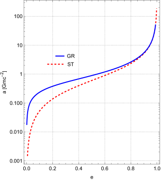
Figure 1: Plot of $a(e)$ at leading order in GR and ST, with geometrical units ($G=c=m=1$). The constant $c_{0}$ is chosen to be $c_{0}=1$ in GR and $c_{0}=(425/304)^{870/2299}\approx 1.135$ in ST theory, such that the asymptotic expressions of $a(e)$ when $e\rightarrow 1$ coincide in both theories.

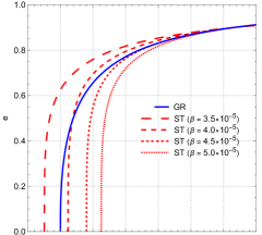
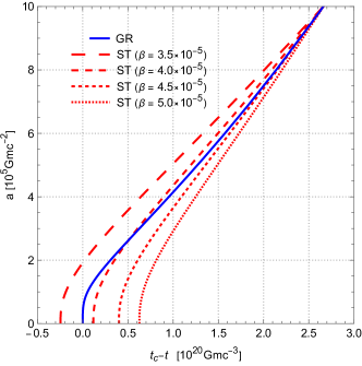
Figure 2: Time evolution for an equal-mass binary at leading order of $e(t)$ and $a(t)$ in GR and ST tensor theories for several values of the parameter $\beta$ (use geometrical units $G=c=m=1$). Time is expressed as the time remaining until coalescence in the GR case. The initial condition are set such that in all theories, the binary’s has an eccentricity $e=0.9$ and a semi-major axis $a_{0.9}=10^{6}$ at some given time $t_{0.9}$ (here, $t_{c}-t_{0.9}\approx 2.659$). In the ST case $\beta=4.0\times 10^{-5}$, the binary circularizes slower than in GR at earlier times $t_{c}-t_{0.9}>t_{c}-t>2\cdot 10^{19}$, and faster than GR at later times $t_{c}-t<2\cdot 10^{19}$.

In order to compare the two functions, switch to geometrical units $G=c=m=1$ for the rest of the subsection. I follow [58] in choosing $c_{0}^{\mathrm{GR}}=1$ in the GR case, and then choose the ST value for $c_{0}$ such that $a(e)$ and $a_{\mathrm{GR}}(e)$ have the same asymptotic behavior as $e\rightarrow 1$. This turns out to be $c_{0}=(425/304)^{\frac{870}{2299}}\approx 1.135$. The two functions $a(e)$ and $a_{\mathrm{GR}}(e)$ are compared in Fig. 1.

One can now plug in the expression (38) for $a(e)$ into (36b), and which leads to an expression analogous to (5.13) of [58] which here reads

$$\left\langle\frac{\differential e}{\differential t}\right\rangle=-\frac{3\beta(1-e^{2})^{3/2}}{4c_{0}^{3}e^{3}}$$ (41)

where

$$\beta=\frac{8}{3}\frac{(\tilde{G}\alpha m)^{2}\zeta\mathcal{S}_{-}^{2}\nu}{c^{3}}\,.$$

Unlike in GR, this ODE is straightforward to integrate, leading to

$$t_{c}-t=\frac{8c_{0}^{3}}{3\beta}\left[\frac{1-e^{2}/2}{\sqrt{1-e^{2}}}-1\right]>0\,,$$ (42)

where $t_{c}$ is an arbitrary constant which is chosen to be the instant of coalescence, such that $a(t)\rightarrow 0$ and $e(t)\rightarrow 0$ when $t\rightarrow t_{c}^{+}$.

This expression is yet again invertable, and its inverse reads

$$e(t)=\sqrt{2(\varrho+1)\sqrt{\varrho(\varrho+2)}-4\varrho-2\varrho^{2}}\,,$$ (43)

where $\varrho\equiv 3\beta(t_{c}-t)/(8c_{0}^{3})>0$. Plugging this expression into (38) directly yields $a(t)$.

To compare the time-evolution of eccentricity in GR and ST, let us plot (42) against the numerically integrated solution of (5.13) of [58]. Consider the case of an equal mass binary, i.e. $\nu=1/4$. Thus, the “$\beta$” defined in [58] is given $\beta_{\mathrm{GR}}=16/5$, while in ST theory $\beta$ is the only free parameter of the theory at this order. Finally, set up the initial condition by imposing that for each theory, there is a common time $t_{0.9}$ where the binary has eccentricity $e=0.9$ and semi-major axis $a_{0.9}=10^{6}$. The time evolution is plotted in Fig. 2. The behavior depends strongly on the choice for the parameter $\beta$, but for certain regimes, the binary initially circularizes slower than in GR, but after some given time, it instead circularizes faster.

V.3 Time evolution of $x$ and $e_{t}$

At next-to-leading, Newtonian order, one cannot obtain closed form expressions for the time-evolution of the orbital elements. In order to avoid clutter, I only present hereafter the evolution of the two main variables used to describe the motion, $x$ and $e_{t}$ (they are also given in machine-readable form in the Supplementary Material [89]). Thanks to the relations displayed in App. C along with (IV.2), the reader can then obtain the secular time-evolution of all the PK orbital elements by simple algebraic replacements. The evolution equations read

$$\left\langle\frac{\differential x}{\differential t}\right\rangle =\frac{2c^{3}\zeta x^{4}\nu}{3\tilde{G}\alpha m}\Bigg{\{}\frac{4\mathcal{S}_{-}^{2}(1+\frac{1}{2}e_{t}^{2})}{(1-e_{t}^{2})^{5/2}}$$

$$+\frac{x}{15(1-e_{t}^{2})^{7/2}}\Big{(}\mathcal{C}_{1}+e_{t}^{2}\mathcal{C}_{2}+e_{t}^{4}\mathcal{C}_{3}\Big{)}+\mathcal{O}(x^{2})\Bigg{\}}\,,$$ (44a)

$$\left\langle\frac{\differential e_{t}}{\differential t}\right\rangle =-\frac{c^{3}\zeta x^{3}\nu}{\tilde{G}\alpha m}\Bigg{\{}\frac{2\mathcal{S}_{-}^{2}e_{t}}{(1-e_{t}^{2})^{3/2}}$$

$$\qquad\quad+\frac{x\,e_{t}}{15(1-e_{t}^{2})^{5/2}}\Big{(}\mathcal{C}_{4}+e_{t}^{2}\mathcal{C}_{5}\Big{)}+\mathcal{O}(x^{2})\Bigg{\}}\,,$$ (44b)

where the constants $\mathcal{C}_{n}$ depend only on the masses and the scalar-tensor parameters, and read

$$\mathcal{C}_{1} =288\bar{\zeta}^{-1}+120\bar{\zeta}^{-1}\bar{\gamma}-30\mathcal{S}_{-}^{2}-160\bar{\beta}_{+}\mathcal{S}_{-}^{2}+240\bar{\beta}_{+}\bar{\gamma}^{-1}\mathcal{S}_{-}^{2}+40\bar{\gamma}\mathcal{S}_{-}^{2}+240\bar{\beta}_{-}\bar{\gamma}^{-1}\mathcal{S}_{-}\mathcal{S}_{+}$$

$$\quad+\delta\Big{(}160\bar{\beta}_{-}\mathcal{S}_{-}^{2}-240\bar{\beta}_{-}\bar{\gamma}^{-1}\mathcal{S}_{-}^{2}-240\bar{\beta}_{+}\bar{\gamma}^{-1}\mathcal{S}_{-}\mathcal{S}_{+}\Big{)}-70\mathcal{S}_{-}^{2}\nu\,,$$ (45a)

$$\mathcal{C}_{2} =876\bar{\zeta}^{-1}+480\bar{\beta}_{+}\bar{\zeta}^{-1}+285\bar{\zeta}^{-1}\bar{\gamma}-720\bar{\beta}_{+}^{2}\bar{\zeta}^{-1}\bar{\gamma}^{-1}+1095\mathcal{S}_{-}^{2}-260\bar{\beta}_{+}\mathcal{S}_{-}^{2}+540\bar{\gamma}\mathcal{S}_{-}^{2}-240\bar{\beta}_{+}\bar{\gamma}^{-1}\mathcal{S}_{-}^{2}$$

$$\quad+1440\bar{\beta}_{-}^{2}\bar{\gamma}^{-2}\mathcal{S}_{-}^{2}+1440\bar{\beta}_{+}^{2}\bar{\gamma}^{-2}\mathcal{S}_{-}^{2}-240\bar{\beta}_{-}\bar{\gamma}^{-1}\mathcal{S}_{-}\mathcal{S}_{+}+2880\bar{\beta}_{-}\bar{\beta}_{+}\bar{\gamma}^{-2}\mathcal{S}_{-}\mathcal{S}_{+}$$

$$\quad+\delta\Big{(}260\bar{\beta}_{-}\mathcal{S}_{-}^{2}-480\bar{\beta}_{-}\bar{\gamma}^{-1}\mathcal{S}_{-}^{2}-480\bar{\beta}_{+}\bar{\gamma}^{-1}\mathcal{S}_{-}\mathcal{S}_{+}\Big{)}-625\mathcal{S}_{-}^{2}\nu\,,$$ (45b)

$$\mathcal{C}_{3} =111\bar{\zeta}^{-1}+120\bar{\beta}_{+}\bar{\zeta}^{-1}+\frac{105}{4}\bar{\zeta}^{-1}\bar{\gamma}-180\bar{\beta}_{+}^{2}\bar{\zeta}^{-1}\bar{\gamma}^{-1}+270\mathcal{S}_{-}^{2}+110\bar{\gamma}\mathcal{S}_{-}^{2}-150\bar{\beta}_{+}\bar{\gamma}^{-1}\mathcal{S}_{-}^{2}+360\bar{\beta}_{-}^{2}\bar{\gamma}^{-2}\mathcal{S}_{-}^{2}$$

$$\quad+360\bar{\beta}_{+}^{2}\bar{\gamma}^{-2}\mathcal{S}_{-}^{2}-150\bar{\beta}_{-}\bar{\gamma}^{-1}\mathcal{S}_{-}\mathcal{S}_{+}+720\bar{\beta}_{-}\bar{\beta}_{+}\bar{\gamma}^{-2}\mathcal{S}_{-}\mathcal{S}_{+}+\delta\Big{(}-30\bar{\beta}_{-}\bar{\gamma}^{-1}\mathcal{S}_{-}^{2}-30\bar{\beta}_{+}\bar{\gamma}^{-1}\mathcal{S}_{-}\mathcal{S}_{+}\Big{)}-130\mathcal{S}_{-}^{2}\nu\,,$$ (45c)

$$\mathcal{C}_{4} =304\bar{\zeta}^{-1}+160\bar{\beta}_{+}\bar{\zeta}^{-1}+100\bar{\zeta}^{-1}\bar{\gamma}-240\bar{\beta}_{+}^{2}\bar{\zeta}^{-1}\bar{\gamma}^{-1}+165\mathcal{S}_{-}^{2}-120\bar{\beta}_{+}\mathcal{S}_{-}^{2}+100\bar{\gamma}\mathcal{S}_{-}^{2}-40\bar{\beta}_{+}\bar{\gamma}^{-1}\mathcal{S}_{-}^{2}+480\bar{\beta}_{-}^{2}\bar{\gamma}^{-2}\mathcal{S}_{-}^{2}$$

$$\quad+480\bar{\beta}_{+}^{2}\bar{\gamma}^{-2}\mathcal{S}_{-}^{2}-40\bar{\beta}_{-}\bar{\gamma}^{-1}\mathcal{S}_{-}\mathcal{S}_{+}+960\bar{\beta}_{-}\bar{\beta}_{+}\bar{\gamma}^{-2}\mathcal{S}_{-}\mathcal{S}_{+}$$

$$\quad+\delta\Big{(}120\bar{\beta}_{-}\mathcal{S}_{-}^{2}-200\bar{\beta}_{-}\bar{\gamma}^{-1}\mathcal{S}_{-}^{2}-200\bar{\beta}_{+}\bar{\gamma}^{-1}\mathcal{S}_{-}\mathcal{S}_{+}\Big{)}-125\mathcal{S}_{-}^{2}\nu\,,$$ (45d)

$$\mathcal{C}_{5} =121\bar{\zeta}^{-1}+40\bar{\beta}_{+}\bar{\zeta}^{-1}+\frac{175}{4}\bar{\zeta}^{-1}\bar{\gamma}-60\bar{\beta}_{+}^{2}\bar{\zeta}^{-1}\bar{\gamma}^{-1}+280\mathcal{S}_{-}^{2}-20\bar{\beta}_{+}\mathcal{S}_{-}^{2}+130\bar{\gamma}\mathcal{S}_{-}^{2}-10\bar{\beta}_{+}\bar{\gamma}^{-1}\mathcal{S}_{-}^{2}+120\bar{\beta}_{-}^{2}\bar{\gamma}^{-2}\mathcal{S}_{-}^{2}$$

$$\quad+120\bar{\beta}_{+}^{2}\bar{\gamma}^{-2}\mathcal{S}_{-}^{2}-10\bar{\beta}_{-}\bar{\gamma}^{-1}\mathcal{S}_{-}\mathcal{S}_{+}+240\bar{\beta}_{-}\bar{\beta}_{+}\bar{\gamma}^{-2}\mathcal{S}_{-}\mathcal{S}_{+}$$

$$\quad+\delta\Big{(}20\bar{\beta}_{-}\mathcal{S}_{-}^{2}-50\bar{\beta}_{-}\bar{\gamma}^{-1}\mathcal{S}_{-}^{2}-50\bar{\beta}_{+}\bar{\gamma}^{-1}\mathcal{S}_{-}\mathcal{S}_{+}\Big{)}-150\mathcal{S}_{-}^{2}\nu\,.$$ (45e)

Solving these ODEs numerically yields the secularly evolving orbital elements $x(t)$ and $e_{t}(t)$, which can be replaced into all results derived in terms of $x$ et $e_{t}$.

VI Waveform

I will now present the waveform for eccentric orbits decomposed into spherical harmonic modes. As in Paper I, the gothic conformal metric is decomposed into two independent modes along the polarization vectors,

$$h_{+} \equiv\frac{1}{2}(P_{i}P_{j}-Q_{i}Q_{j})h_{ij}^{TT}\,,$$ (46a)

$$h_{\times} \equiv\frac{1}{2}(P_{i}Q_{j}+Q_{i}P_{j})h_{ij}^{TT}\,,$$ (46b)

which can be recast into a complex field, $h=h_{+}-\mathrm{i}h_{\times}$. The latter can be decomposed on the basis on spin-weighted spherical harmonics of weight $-2$,

$$h=h_{+}-\mathrm{i}h_{-}=\sum_{\ell=2}^{+\infty}\sum_{m=-\ell}^{\ell}h^{\ell m}\,_{-2}Y^{\ell m}(\Theta,\Phi)\,.$$ (47a)

Similarly, the pure spin-0 scalar field can be decomposed on standard (spin-0) spherical harmonics,

$$\psi=\sum_{\ell=0}^{+\infty}\sum_{m=-\ell}^{\ell}\psi^{\ell m}\ Y^{\ell m}(\Theta,\Phi)\,.$$ (47b)

The modes are in practice computed using the relations

$$h^{\ell m} =-\frac{G}{\sqrt{2}Rc^{\ell+2}}\Big{[}\mathcal{U}^{\ell m}-\frac{\mathrm{i}}{c}\mathcal{V}^{\ell m}\Big{]}\,,$$ (48a)

$$\psi^{\ell m} =\frac{G}{Rc^{\ell+2}}\mathcal{U}_{s}^{\ell m}\,,$$ (48b)

where

$$\mathcal{U}^{\ell m} =\frac{4}{\ell!}\sqrt{\frac{(\ell+1)(\ell+2)}{2\ell(\ell-1)}}\alpha_{L}^{\ell m}\mathcal{U}_{L}\,,$$ (49a)

$$\mathcal{V}^{\ell m} =-\frac{8}{\ell!}\sqrt{\frac{\ell(\ell+2)}{2(\ell+1)(\ell-1)}}\alpha_{L}^{\ell m}\mathcal{V}_{L}\,,$$ (49b)

$$\mathcal{U}_{s}^{\ell m} =-\frac{2}{\ell!}\alpha_{L}^{\ell m}\mathcal{U}^{s}_{L}\,,$$ (49c)

and where $\alpha_{L}^{\ell m}$ is defined by

$$\alpha_{L}^{\ell m} \equiv\int\differential\Omega\,\hat{N}_{L}{\left(Y^{\ell m}\right)}^{*}$$ (50)

These modes can then be recast into dimensionless amplitude modes $h^{\ell m}$ and $\psi^{\ell m}$ which are given by

$$h^{\ell m} =\frac{2\tilde{G}(1-\zeta)m\nu x}{Rc^{2}}\sqrt{\frac{16\pi}{5}}\,\hat{H}^{\ell m}\mathrm{e}^{-\mathrm{i}\mathrm{m}\phi}\,,$$ (51a)

$$\psi^{\ell m} =\frac{2i\tilde{G}\zeta\sqrt{\alpha}\mathcal{S}_{-}m\nu\sqrt{x}}{Rc^{2}}\sqrt{\frac{8\pi}{3}}\,\hat{\Psi}^{\ell m}\mathrm{e}^{-\mathrm{i}\mathrm{m}\phi}\,.$$ (51b)

with normalized modes defined such that the expression for circular orbits reads $\hat{H}^{22}_{\mathrm{circ}}=1+\mathcal{O}(x)$ and $\hat{\Psi}^{11}_{\mathrm{circ}}=1+\mathcal{O}({x})$. Recalling that $h^{\ell,-m}=(-)^{\ell}{\left(h^{\ell m}\right)}^{*}$ and $\psi^{\ell,-m}=(-)^{\ell}{\left(\psi^{\ell m}\right)}^{*}$, only the $m\geq 0$ modes that enter the Newtonian (next-to-leading) waveform are presented. In the eccentric case, they exhibit time-oscillations which enter via the eccentric anomaly $u$, see the Kepler equation (18b). They are given in machine-readable form in the Supplementary Material [89], and read:

$$\hat{\Psi}^{00} =-\frac{\mathrm{i}}{\sqrt{x}\mathcal{S}_{-}}\sqrt{\frac{3}{2}}\Bigg{\{}\frac{\mathcal{S}_{+}+\mathcal{S}_{-}\delta}{\nu}+\frac{x}{1-e_{t}\cos u}$$

$$\qquad\quad\times\bigg{[}8\bar{\beta}_{-}\bar{\gamma}^{-1}\mathcal{S}_{-}-\frac{5}{2}\mathcal{S}_{+}+8\bar{\beta}_{+}\bar{\gamma}^{-1}\mathcal{S}_{+}+\frac{1}{2}\mathcal{S}_{-}\delta$$

$$\qquad\qquad\qquad-\frac{e_{t}\cos u}{6}\Big{(}\mathcal{S}_{+}-\mathcal{S}_{-}\delta\Big{)}\bigg{]}\Bigg{\}}+\mathcal{O}(x)$$ (52a)

$$\hat{\Psi}^{11} =\frac{1-e_{t}^{2}-\mathrm{i}e_{t}\sqrt{1-e_{t}^{2}}\sin u}{\sqrt{1-e_{t}^{2}}(1-e_{t}\cos u)}+\mathcal{O}(x)$$ (52b)

$$\hat{\Psi}^{22} =\frac{\mathrm{i}\sqrt{x}\left(\mathcal{S}_{+}-\mathcal{S}_{-}\delta\right)}{\sqrt{5}\mathcal{S}_{-}(1-\cos u)^{2}}\Bigg{\{}1-\frac{1}{2}e_{t}\cos u$$

$$\quad+\frac{1}{4}e_{t}^{2}\left(-3+\cos 2u\right)-\mathrm{i}e_{t}\sqrt{1-e_{t}^{2}}\sin u\Bigg{\}}+\mathcal{O}(x)$$ (52c)

$$\hat{\Psi}^{20} =\frac{\mathrm{i}\sqrt{x}e_{t}\cos u\left(\mathcal{S}_{+}-\mathcal{S}_{-}\delta\right)}{\sqrt{30}\mathcal{S}_{-}(1-e_{t}\cos u)}$$ (52d)

$$\hat{H}^{22} =\frac{1}{(1-e_{t}\cos u)^{2}}\Bigg{\{}1-\frac{1}{2}e_{t}\cos u$$

$$\quad+\frac{1}{4}e_{t}^{2}\left(-3+\cos 2u\right)-\mathrm{i}e_{t}\sqrt{1-e_{t}^{2}}\sin u\Bigg{\}}+\mathcal{O}(x)$$ (52e)

$$\hat{H}^{20} =\frac{e_{t}\cos u}{\sqrt{6}(1-e_{t}\cos u)}+\mathcal{O}(x)$$ (52f)

These results agree in the GR limit with [73], as well as with Paper I in the circular $e_{t}\rightarrow 0$ limit.

VII Conclusion

To my knowledge, this work is the first systematic analytical study of eccentric binaries in ST theories. The expressions of the 2PK orbital elements were computed, first in a generic setting, then specializing to ST theories. The flux of energy and angular momentum at next-to-leading order beyond dipolar radiation were then derived, i.e. at Newtonian order with respect to quadrupolar radiation. After a preliminary study of the leading order $-1$PN case, for which were obtained several closed form expressions analogous to the works of Peters and Matthews [57, 58], the energy and angular momentum balance equations were then used to obtain the ODEs expressing the secular evolution of the orbital elements at Newtonian order. Finally, the expressions for waveform in terms of spherical harmonic modes were computed at Newtonian order. At all steps of these computations, I checked that these results were in agreement with the literature in the GR limit as well in limiting case of circular orbits ($e_{t}\rightarrow 0$).

Thanks to the 2PK parametrization computed in this work, it is in principle possible to obtain the fluxes, waveform and evolution of the orbital elements at 1.5PN order, just like in Paper I. However, one difficulty for this is the treatment of the hereditary tail and memory integrals in the eccentric case. In GR, it is possible to treat these analytically [70, 71, 72] as an expansion in eccentricity for $e_{t}\ll 1$, and the generalization to the case of ST would not present any additional difficulty. Another possible extension of this work is the derivation of the 3PK parametrization. The main difficulty would be the treatment of the nonlocal tails in the equations and conserved energy. Extending the techniques developed for GR at 4PN order to treat these hereditary terms [63] seems possible as well.

Finally, I would like to emphasize that the results of Sec. III.1 are not theory dependent: they can be used as soon as one obtains an expression for the energy and angular momentum that exhibits the right properties. These results are to be used as a facilitator in studying the behavior of compact binary systems on eccentric orbits for a range of different theories of gravity.

Appendix A Integration formulas using complex analysis

The goal of this section is to sketch the computation of integrals of the type (16). It was proven that the PN expansion of these integrals can readily be performed by integrating the PN expansion of the integrand [60]. Since $D_{1}$, $D_{2}$ and $D_{3}$ are all small in the PN sense, with the help of (15), both integrals of (16) can be written in the form

$$\sum_{k\in\mathbb{N}}\int_{s_{a}}^{s_{p}}\frac{\differential s\,\overline{P}_{k}(s)}{s^{2}\Big{\{}A+2Bs+Cs^{2}\Big{\}}^{k/2}}\,,$$ (53)

where $\overline{P}_{k}(s)$ is a polynomial that arises from the PN expansion of the integrand. This naturally leads to posing the master integral

$$\mathcal{I}_{p,q}=\frac{1}{\pi}\int_{s_{a}}^{s_{p}}\differential s\,s^{p-2}\left(A+2Bs+Cs^{2}\right)^{1/2-q}\,,$$ (54)

where $(p,q)\in\mathbb{N}^{2}$, and recall that $A<0$, $B>0$ and $C<0$. Following a method initially found by Sommerfeld [94], this integral is astutely promoted into a path integral in the complex plane [95, 60]:

$$\mathcal{I}_{p,q}=\frac{1}{2\pi}\oint_{\mathcal{C}}\differential s\,s^{p-2}\left(A+2Bs+Cs^{2}\right)^{1/2-q}\,.$$ (55)

Figure 3: Sketch of the integration contours $\mathcal{C}$, $\mathcal{C}_{0}$ and $\mathcal{C}_{\infty}$, adapted from [96]. The integrand of (55) exhibits poles at $0$ and $\infty$, and is meromorphic everywhere except in the neighborhood of the segment $[s_{a},s_{p}]$.

The contour $\mathcal{C}$ loops counterclockwise around the two roots $s_{a}$ and $s_{p}$, avoiding the poles at $s=0$, see Fig. 3. The integrand is not meromorphic inside of $\mathcal{C}$, so the residue theorem cannot be directly applied. However, it is possible to deform the contour into $\mathcal{C}_{0}$ and $\mathcal{C}_{\infty}$, which respectively contain the pole at $0$ and $\infty$ (the pole at infinity is mapped back to $0$ thanks to the change of variables $r=1/s$). The integrands are now meromorphic within the contours, so the residue theorem is applied. The end result reads

$$\mathcal{I}_{p,q} =\big{[}p=0\big{]}(-1)^{q}(1-2q)B(-A)^{-1/2-q}$$

$$+\big{[}p=1\big{]}(-1)^{q+1}(-A)^{1/2-q}$$

$$+\big{[}p\geq 2q\big{]}(-1)^{q+1}(-C)^{1/2-q}$$

$$\!\!\!\!\!\times\!\!\!\!\!\!\sum_{k=\lceil\frac{p}{2}-q\rceil}^{p-2q}\!\!\frac{\Gamma\left(\frac{1}{2}-q+1\right)A^{p-k-2q}\,(2B)^{2k+2q-p}\,C^{-k}}{\Gamma\left(\frac{1}{2}-q-k+1\right)(2k+2q-p)!(p-k-2q)!}\,,$$ (56)

where $\Gamma(x)$ is the usual gamma function, $\lceil n\rceil$ is the ceiling of the integer $n$, and $\big{[}\mathcal{P}\big{]}$ is the Inverson bracket defined such that $[\mathcal{P}]=1$ if $\mathcal{P}$ is true, and $[\mathcal{P}]=0$ otherwise. When applied to (3.8) of [60], this formula yields indeed the correct result, given by (3.9) of [60].

Appendix B Details of the post-Keplerian construction at 2PN order

The starting point of the determination of the PK parametrization is (13). The periods $P$ and $K$ defined by (16) are obtained using the techniques of App. A, from which one trivially obtains the mean motion $n=2\pi/P$. The positions of the periastron $r_{p}$ and apastron $r_{a}$ are first obtained at lowest order by factorizing the $c\rightarrow\infty$ limit of $\mathcal{R}(s)$. PN corrections to these roots are then obtained iteratively by requiring that they cancel $\mathcal{R}(s)$, up to higher-order PN corrections. The PK parameters $a_{r}=(s_{p}+s_{a})/(2s_{a}s_{p})$ and $e_{r}=(s_{p}-s_{a})/(s_{p}+s_{a})$ are then trivial to obtain, where we recall $s_{p,a}=1/r_{p,a}$. Following [62], it is now very useful to introduce the auxiliary variable

$$\tilde{v}\equiv 2\arctan\left(\sqrt{\frac{1+e_{r}}{1-e_{r}}}\tan\left(\frac{u}{2}\right)\right)\,,$$ (57)

which differs from $v$ defined in (19) by the choice of eccentricity. Note that at this stage, $e_{\phi}$ and $e_{t}$ are undetermined, only $e_{r}$ is known.

The starting point to determine the Kepler equation is

$$t-t_{0}=2\int_{s}^{s_{p}}\frac{\differential s}{s^{2}\sqrt{\mathcal{R}(s)}}=2\int_{s}^{s_{p}}\frac{\differential s\,\overline{P}(s)}{s^{2}\sqrt{(s-s_{p})(s-s_{a})}}\,,$$ (58)

where $\overline{P}(s)$ arises (similarly to (53)) from the PN expansion of $1/\sqrt{\widetilde{\mathcal{R}}\smash{(s)}}$, see (15). The problem has now been reduced to computing master integrals of the form

$$\mathcal{J}_{p}\equiv\int_{s}\frac{\differential s\,s^{p-2}}{\sqrt{(s-s_{a})(s-s_{p})}}\,,$$ (59)

Interestingly, these master integrals are most conveniently expressed using auxiliary variables that depend heavily on the value of $p$. They are given by

$$\mathcal{J}_{0} =\frac{(s_{a}+s_{p})u-(s_{p}-s_{a})\sin(u)}{2(s_{a}s_{p})^{3/2}}$$ (60a)

$$\mathcal{J}_{1} =\frac{u}{\sqrt{s_{a}s_{p}}}$$ (60b)

$$\mathcal{J}_{2} =\tilde{v}$$ (60c)

$$\mathcal{J}_{3} =\frac{(s_{a}+s_{p})\tilde{v}+(s_{p}-s_{a})\sin(\tilde{v})}{2}$$ (60d)

$$\mathcal{J}_{4} =\frac{3s_{a}^{2}+2s_{a}s_{p}+3s_{p}^{2}}{8}\tilde{v}+\frac{(s_{p}-s_{a})(s_{p}+s_{a})}{2}\sin(\tilde{v})$$

$$\quad+\frac{(s_{p}-s_{a})^{2}}{16}\sin(2\tilde{v})$$ (60e)

$$\mathcal{J}_{5} =\frac{(s_{p}+s_{a})(5s_{a}^{2}-2s_{a}s_{p}+5s_{p}^{2})}{16}\tilde{v}$$

$$\quad+\frac{3(s_{p}-s_{a})(5s_{a}^{2}+6s_{a}s_{p}+5s_{p}^{2})}{32}\sin(\tilde{v})$$

$$\quad+\frac{3(s_{p}-s_{a})^{2}(s_{a}+s_{p})}{32}\sin(2\tilde{v})$$

$$\quad+\frac{(s_{p}-s_{a})^{3}}{96}\sin(3\tilde{v})$$ (60f)

Keeping with the notation of [62], and replacing $s_{p}$ and $s_{a}$ by their 2PN accurate expressions, I explicitly find an intermediate form for the Kepler equation,

$$n(t-t_{0})=u+\kappa_{0}\sin(u)+\frac{\kappa_{1}}{c^{2}}(\tilde{v}-u)+\frac{\kappa_{2}}{c^{4}}\sin(\tilde{v})\,.$$ (61)

Similarly, the computation of the angular equation starts from the integral

$$\phi-\phi_{0}=2\int_{s}^{s_{p}}\frac{\differential s\,\mathcal{S}(s)}{s^{2}\sqrt{\mathcal{R}(s)}}=2\int_{s}^{s_{p}}\frac{\differential s\,\overline{Q}(s)}{s^{2}\sqrt{(s-s_{p})(s-s_{a})}}\,,$$ (62)

where $\overline{Q}(s)$ arises from the PN expansion of $\mathcal{S}(s)/\sqrt{\tilde{R}\smash{(s)}}$. The master integrals of (60) apply, and we find the explicit intermediate form of the angular equation to be

$$\frac{2\pi}{\Phi}=\tilde{v}+\frac{\lambda_{1}}{c^{2}}\sin(\tilde{v})+\frac{\lambda_{2}}{c^{4}}\sin(2\tilde{v})+\frac{\lambda_{3}}{c^{4}}\sin(3\tilde{v})\,.$$ (63)

Let us now turn to the problem of expressing the Kepler and angular equations in terms of $v$. First, parametrize the 2PN-accurate relation between $e_{r}$ and $e_{\phi}$ as

$$e_{r}=e_{\phi}\left(1+\frac{\alpha}{c^{2}}+\frac{\beta}{c^{4}}\right)\,,$$ (64)

and Taylor-expand Eq. (57). To this end, first write

$$\sqrt{\frac{1+e_{r}}{1-e_{r}}}=\sqrt{\frac{1+e_{\phi}}{1-e_{\phi}}}\left(1+\frac{\kappa}{c^{2}}\right)\,,$$ (65)

where

$$\kappa=\frac{\alpha e_{\phi}}{(1-e_{\phi}^{2})}+\frac{e_{\phi}(2\beta+\alpha^{2}e_{\phi}+2e_{\phi}^{2}(\alpha^{2}-\beta)}{2c^{2}(1-e_{\phi}^{2})^{2}}+\mathcal{O}\left(\frac{1}{c^{4}}\right)\,.$$ (66)

Then, thanks to the identities

$$\arctan^{\prime}(x) =\frac{\sin(2\arctan(x))}{2x}\,,$$ (67a)

$$\arctan^{\prime\prime}(x) =\frac{\sin(4\arctan(x))-2\sin(2\arctan(x))}{4x^{2}}\,,$$ (67b)

the relation between $\tilde{v}$ and $v$ can then be written

$$\tilde{v}=v+\frac{\kappa}{c^{2}}\sin(v)+\frac{\kappa^{2}}{4c^{4}}\left(\sin(2v)-2\sin(v)\right)+\mathcal{O}\left(\frac{1}{c^{6}}\right)\,.$$ (68)

Moreover, the latter relation immediately leads to

$$\sin(\tilde{v})=\sin(v)+\frac{\kappa}{2c^{2}}\sin(2v)+\mathcal{O}\left(\frac{1}{c^{4}}\right)\,.$$ (69)

Replacing these relations into the intermediate angular relation (63), one obtains an equation with the same form as (18c), except that there is an extra term proportional to $\sin(v)$. Now is the time to use the freedom in $\alpha$ and $\beta$ to set the coefficient in front of $\sin(v)$ to zero. In this way, the relation (64) between $e_{\phi}$ and $e_{r}$ is entirely determined. Finally, since the intermediate Kepler equation (61) only features $\tilde{v}$ at 2PN order, one can simply replace it by $v$ so as to obtain exactly the form of (18b). It is then straightforward to simply read off all the PK parameters.

Appendix C Expressions for post-Keplerian parameters in massless scalar-tensor theories

The post-Keplerian parameters in terms of $\varepsilon$, $j$ and the ST parameters are given in machine-readable form in the Supplementary Material [89], and are presented hereafter as well.

$$n =\frac{c^{3}\varepsilon^{3/2}}{\tilde{G}\alpha m}\Bigg{\{}1+\varepsilon\Bigg{[}-\frac{15}{8}-\bar{\gamma}+\frac{\nu}{8}\Bigg{]}$$

$$\qquad+\varepsilon^{2}\Bigg{[}\frac{555}{128}+\frac{33}{8}\bar{\gamma}+\bar{\gamma}^{2}+\nu\left(\frac{15}{64}+\frac{1}{8}\bar{\gamma}\right)+\frac{11}{128}\nu^{2}+\frac{-15(1+\bar{\gamma}+\frac{\bar{\gamma}^{2}}{4})+\bar{\delta}_{+}+\bar{\delta}_{-}\delta+\nu\Big{(}6-2\bar{\beta}_{+}+4\bar{\gamma}+2\bar{\beta}_{-}\delta\Big{)}}{2\sqrt{j}}\Bigg{]}\Bigg{\}}$$ (70a)

$$K =1+\frac{\varepsilon}{j}\Big{[}3-\bar{\beta}_{+}+2\bar{\gamma}+\bar{\beta}_{-}\delta\Big{]}$$

$$\qquad+\frac{\varepsilon^{2}}{j^{2}}\Bigg{[}\frac{105}{4}+\frac{3}{2}\bar{\beta}_{-}^{2}-15\bar{\beta}_{+}+\frac{3}{2}\bar{\beta}_{+}^{2}-\frac{5}{4}\bar{\delta}_{+}+\frac{139}{4}\bar{\gamma}-12\bar{\beta}_{+}\bar{\gamma}+\frac{187}{16}\bar{\gamma}^{2}-2\bar{\chi}_{+}$$

$$\qquad\qquad\quad+\delta\Big{(}15\bar{\beta}_{-}-3\bar{\beta}_{-}\bar{\beta}_{+}-\frac{5}{4}\bar{\delta}_{-}+12\bar{\beta}_{-}\bar{\gamma}+2\bar{\chi}_{-}\Big{)}$$

$$\qquad\qquad\quad+\nu\Big{(}-\frac{15}{2}-6\bar{\beta}_{-}^{2}+\frac{21}{2}\bar{\beta}_{+}-2\bar{\delta}_{+}-8\bar{\gamma}-\frac{1}{2}\bar{\gamma}^{2}+24\bar{\beta}_{-}^{2}\bar{\gamma}^{-1}-24\bar{\beta}_{+}^{2}\bar{\gamma}^{-1}+4\bar{\chi}_{+}-\frac{3}{2}\bar{\beta}_{-}\delta\Big{)}$$

$$\qquad\qquad\quad+j\Bigg{(}-\frac{15}{4}+\frac{1}{4}\bar{\delta}_{+}-\frac{15}{4}\bar{\gamma}-\frac{15}{16}\bar{\gamma}^{2}+\frac{1}{4}\bar{\delta}_{-}\delta+\nu\Big{(}\frac{3}{2}-\frac{1}{2}\bar{\beta}_{+}+\bar{\gamma}+\frac{1}{2}\bar{\beta}_{-}\delta\Big{)}\Bigg{)}\Bigg{]}$$ (70b)

$$a_{r} =\frac{\tilde{G}\alpha m}{c^{2}\varepsilon}\Bigg{\{}1+\varepsilon\Bigg{[}-\frac{7}{4}-\bar{\gamma}+\frac{1}{4}\nu\Bigg{]}$$

$$\qquad\qquad\ \ +\varepsilon^{2}\Bigg{[}\frac{1+\nu^{2}}{16}+\frac{1}{j}\Bigg{(}-4+2\bar{\beta}_{+}+\frac{2}{3}\bar{\delta}_{+}-\frac{16}{3}\bar{\gamma}+2\bar{\beta}_{+}\bar{\gamma}-\frac{11}{6}\bar{\gamma}^{2}+\frac{2}{3}\bar{\chi}_{+}+\delta\Big{(}-2\bar{\beta}_{-}+\frac{2}{3}\bar{\delta}_{-}-2\bar{\beta}_{-}\bar{\gamma}-\frac{2}{3}\bar{\chi}_{-}\Big{)}$$

$$\qquad\qquad\qquad\qquad\qquad\qquad\quad+\nu\Big{(}7-5\bar{\beta}_{+}+\frac{2}{3}\bar{\delta}_{+}+\frac{17}{3}\bar{\gamma}+\frac{1}{6}\bar{\gamma}^{2}-8\bar{\beta}_{-}^{2}\bar{\gamma}^{-1}+8\bar{\beta}_{+}^{2}\bar{\gamma}^{-1}-\frac{4}{3}\bar{\chi}_{+}+\bar{\beta}_{-}\delta\Big{)}\Bigg{)}\Bigg{]}\Bigg{\}}$$ (70c)

$$e_{r} =\sqrt{1-j}\Bigg{\{}1+\frac{\varepsilon}{1-j}\Bigg{[}3-\bar{\beta}_{+}+2\bar{\gamma}+\bar{\beta}_{-}\delta-\frac{1}{2}\nu+j\Bigg{(}-\frac{15}{8}-\bar{\gamma}+\frac{5}{8}\nu\Bigg{)}\Bigg{]}$$

$$\qquad\qquad\ \ +\frac{\varepsilon^{2}}{(1-j)^{2}}\Bigg{[}-\frac{35}{4}-\frac{1}{2}\bar{\beta}_{-}^{2}+\frac{21}{4}\bar{\beta}_{+}-\frac{1}{2}\bar{\beta}_{+}^{2}+\frac{5}{2}\bar{\delta}_{+}-12\bar{\gamma}+6\bar{\beta}_{+}\bar{\gamma}-\frac{35}{8}\bar{\gamma}^{2}+2\bar{\chi}_{+}$$

$$\qquad\qquad\qquad\qquad\qquad+\delta\Big{(}-\frac{21}{4}\bar{\beta}_{-}+\bar{\beta}_{-}\bar{\beta}_{+}+\frac{5}{2}\bar{\delta}_{-}-6\bar{\beta}_{-}\bar{\gamma}-2\bar{\chi}_{-}\Big{)}$$

$$\qquad\qquad\qquad\qquad\qquad+\nu\Big{(}\frac{99}{4}+2\bar{\beta}_{-}^{2}-\frac{65}{4}\bar{\beta}_{+}+2\bar{\delta}_{+}+\frac{39}{2}\bar{\gamma}+\frac{1}{2}\bar{\gamma}^{2}-24\bar{\beta}_{-}^{2}\bar{\gamma}^{-1}+24\bar{\beta}_{+}^{2}\bar{\gamma}^{-1}-4\bar{\chi}_{+}+\frac{13}{4}\bar{\beta}_{-}\delta\Big{)}$$

$$\qquad\qquad\qquad\qquad+\frac{1}{j}\Bigg{(}8-4\bar{\beta}_{+}-\frac{4}{3}\bar{\delta}_{+}+\frac{32}{3}\bar{\gamma}-4\bar{\beta}_{+}\bar{\gamma}+\frac{11}{3}\bar{\gamma}^{2}-\frac{4}{3}\bar{\chi}_{+}+\delta\Big{(}4\bar{\beta}_{-}-\frac{4}{3}\bar{\delta}_{-}+4\bar{\beta}_{-}\bar{\gamma}+\frac{4}{3}\bar{\chi}_{-}\Big{)}$$

$$\qquad\qquad\qquad\qquad\qquad+\nu\Big{(}-14+10\bar{\beta}_{+}-\frac{4}{3}\bar{\delta}_{+}-\frac{34}{3}\bar{\gamma}-\frac{1}{3}\bar{\gamma}^{2}+16\bar{\beta}_{-}^{2}\bar{\gamma}^{-1}-16\bar{\beta}_{+}^{2}\bar{\gamma}^{-1}+\frac{8}{3}\bar{\chi}_{+}-2\bar{\beta}_{-}\delta\Big{)}\Bigg{)}$$

$$\qquad\qquad\qquad\qquad+j\Bigg{(}-\frac{25}{8}-\frac{1}{8}\bar{\beta}_{+}-\frac{7}{6}\bar{\delta}_{+}-\frac{41}{12}\bar{\gamma}-\bar{\beta}_{+}\bar{\gamma}-\frac{19}{24}\bar{\gamma}^{2}-\frac{2}{3}\bar{\chi}_{+}+\delta\Big{(}\frac{1}{8}\bar{\beta}_{-}-\frac{7}{6}\bar{\delta}_{-}+\bar{\beta}_{-}\bar{\gamma}+\frac{2}{3}\bar{\chi}_{-}\Big{)}$$

$$\qquad\qquad\qquad\qquad\qquad+\nu\Big{(}-\frac{37}{4}+\frac{51}{8}\bar{\beta}_{+}-\frac{2}{3}\bar{\delta}_{+}-\frac{89}{12}\bar{\gamma}-\frac{1}{6}\bar{\gamma}^{2}+8\bar{\beta}_{-}^{2}\bar{\gamma}^{-1}-8\bar{\beta}_{+}^{2}\bar{\gamma}^{-1}+\frac{4}{3}\bar{\chi}_{+}-\frac{11}{8}\bar{\beta}_{-}\delta\Big{)}-\frac{1}{16}\nu^{2}\Bigg{)}$$

$$\qquad\qquad\qquad\qquad+j^{2}\Bigg{(}\frac{415}{128}+\frac{29}{8}\bar{\gamma}+\bar{\gamma}^{2}+\nu\Big{(}-\frac{105}{64}-\frac{7}{8}\bar{\gamma}\Big{)}+\frac{7}{128}\nu^{2}\Bigg{)}\Bigg{]}\Bigg{\}}$$ (70d)

$$e_{t} =\sqrt{1-j}\Bigg{\{}1+\frac{\varepsilon}{1-j}\Bigg{[}-1-\bar{\beta}_{+}+\bar{\beta}_{-}\delta+\nu+j\Bigg{(}\frac{17}{8}+\bar{\gamma}-\frac{7}{8}\nu\Bigg{)}\Bigg{]}$$

$$\qquad\qquad\qquad\ \ +\frac{\varepsilon^{2}}{\sqrt{j}}\Bigg{[}-\frac{15}{2}+\frac{1}{2}\bar{\delta}_{+}-\frac{15}{2}\bar{\gamma}-\frac{15}{8}\bar{\gamma}^{2}+\frac{1}{2}\bar{\delta}_{-}\delta+\nu\Big{(}3-\bar{\beta}_{+}+2\bar{\gamma}+\bar{\beta}_{-}\delta\Big{)}\Bigg{]}$$

$$\qquad\qquad\ \ +\frac{\varepsilon^{2}}{(1-j)^{2}}\Bigg{[}-\frac{15}{4}-\frac{1}{2}\bar{\beta}_{-}^{2}+\frac{21}{4}\bar{\beta}_{+}-\frac{1}{2}\bar{\beta}_{+}^{2}+\frac{7}{6}\bar{\delta}_{+}-\frac{41}{6}\bar{\gamma}+4\bar{\beta}_{+}\bar{\gamma}-\frac{65}{24}\bar{\gamma}^{2}+\frac{2}{3}\bar{\chi}_{+}$$

$$\qquad\qquad\qquad\qquad\qquad+\delta\Big{(}-\frac{21}{4}\bar{\beta}_{-}+\bar{\beta}_{-}\bar{\beta}_{+}+\frac{7}{6}\bar{\delta}_{-}-4\bar{\beta}_{-}\bar{\gamma}-\frac{2}{3}\bar{\chi}_{-}\Big{)}+\frac{3}{4}\nu^{2}$$

$$\qquad\qquad\qquad\qquad\qquad+\nu\Big{(}\frac{25}{2}+2\bar{\beta}_{-}^{2}-\frac{31}{4}\bar{\beta}_{+}+\frac{2}{3}\bar{\delta}_{+}+\frac{29}{3}\bar{\gamma}+\frac{1}{6}\bar{\gamma}^{2}-8\bar{\beta}_{-}^{2}\bar{\gamma}^{-1}+8\bar{\beta}_{+}^{2}\bar{\gamma}^{-1}-\frac{4}{3}\bar{\chi}_{+}+\frac{11}{4}\bar{\beta}_{-}\delta\Big{)}$$

$$\qquad\qquad\qquad\qquad+\frac{1}{j}\Bigg{(}4-2\bar{\beta}_{+}-\frac{2}{3}\bar{\delta}_{+}+\frac{16}{3}\bar{\gamma}-2\bar{\beta}_{+}\bar{\gamma}+\frac{11}{6}\bar{\gamma}^{2}-\frac{2}{3}\bar{\chi}_{+}+\delta\Big{(}2\bar{\beta}_{-}-\frac{2}{3}\bar{\delta}_{-}+2\bar{\beta}_{-}\bar{\gamma}+\frac{2}{3}\bar{\chi}_{-}\Big{)}$$

$$\qquad\qquad\qquad\qquad\qquad+\nu\Big{(}-7+5\bar{\beta}_{+}-\frac{2}{3}\bar{\delta}_{+}-\frac{17}{3}\bar{\gamma}-\frac{1}{6}\bar{\gamma}^{2}+8\bar{\beta}_{-}^{2}\bar{\gamma}^{-1}-8\bar{\beta}_{+}^{2}\bar{\gamma}^{-1}+\frac{4}{3}\bar{\chi}_{+}-\bar{\beta}_{-}\delta\Big{)}\Bigg{)}$$

$$\qquad\qquad\qquad\qquad+j\Bigg{(}-\frac{45}{8}-\frac{17}{8}\bar{\beta}_{+}-\frac{1}{2}\bar{\delta}_{+}-4\bar{\gamma}-\bar{\beta}_{+}\bar{\gamma}-\frac{5}{8}\bar{\gamma}^{2}+\delta\Big{(}\frac{17}{8}\bar{\beta}_{-}-\frac{1}{2}\bar{\delta}_{-}+\bar{\beta}_{-}\bar{\gamma}\Big{)}$$

$$\qquad\qquad\qquad\qquad\qquad+\nu\Big{(}-\frac{73}{16}+\frac{23}{8}\bar{\beta}_{+}-\frac{7}{2}\bar{\gamma}-\frac{15}{8}\bar{\beta}_{-}\delta\Big{)}-\frac{11}{8}\nu^{2}\Bigg{)}$$

$$\qquad\qquad\qquad\qquad+j^{2}\Bigg{(}\frac{607}{128}+\frac{35}{8}\bar{\gamma}+\bar{\gamma}^{2}+\nu\Big{(}-\frac{69}{64}-\frac{5}{8}\bar{\gamma}\Big{)}+\frac{79}{128}\nu^{2}\Bigg{)}\Bigg{]}\Bigg{\}}$$ (70e)

$$e_{\phi} =\sqrt{1-j}\Bigg{\{}1+\frac{\varepsilon}{1-j}\Bigg{[}3-\bar{\beta}_{+}+2\bar{\gamma}+\bar{\beta}_{-}\delta+j\Bigg{(}-\frac{15}{8}-\bar{\gamma}+\frac{1}{8}\nu\Bigg{)}\Bigg{]}$$

$$\qquad\qquad\ \ +\frac{\varepsilon^{2}}{(1-j)^{2}}\Bigg{[}-\frac{75}{4}-\frac{1}{2}\bar{\beta}_{-}^{2}+\frac{37}{4}\bar{\beta}_{+}-\frac{1}{2}\bar{\beta}_{+}^{2}+\frac{11}{6}\bar{\delta}_{+}-\frac{74}{3}\bar{\gamma}+10\bar{\beta}_{+}\bar{\gamma}-\frac{205}{24}\bar{\gamma}^{2}+\frac{10}{3}\bar{\chi}_{+}$$

$$\qquad\qquad\qquad\qquad\qquad+\delta\Big{(}-\frac{37}{4}\bar{\beta}_{-}+\bar{\beta}_{-}\bar{\beta}_{+}+\frac{11}{6}\bar{\delta}_{-}-10\bar{\beta}_{-}\bar{\gamma}-\frac{10}{3}\bar{\chi}_{-}\Big{)}+\frac{33}{32}\nu^{2}$$

$$\qquad\qquad\qquad\qquad\qquad+\nu\Big{(}\frac{125}{32}+2\bar{\beta}_{-}^{2}-\frac{59}{4}\bar{\beta}_{+}+\frac{10}{3}\bar{\delta}_{+}+\frac{47}{6}\bar{\gamma}+\frac{5}{6}\bar{\gamma}^{2}-40\bar{\beta}_{-}^{2}\bar{\gamma}^{-1}+40\bar{\beta}_{+}^{2}\bar{\gamma}^{-1}-\frac{20}{3}\bar{\chi}_{+}+\frac{7}{4}\bar{\beta}_{-}\delta\Big{)}$$

$$\qquad\qquad\qquad\qquad+j\Bigg{(}\frac{15}{8}-\frac{17}{8}\bar{\beta}_{+}-\frac{5}{6}\bar{\delta}_{+}+\frac{35}{12}\bar{\gamma}-3\bar{\beta}_{+}\bar{\gamma}+\frac{31}{24}\bar{\gamma}^{2}-\frac{4}{3}\bar{\chi}_{+}+\delta\Big{(}\frac{17}{8}\bar{\beta}_{-}-\frac{5}{6}\bar{\delta}_{-}+3\bar{\beta}_{-}\bar{\gamma}+\frac{4}{3}\bar{\chi}_{-}\Big{)}$$

$$\qquad\qquad\qquad\qquad\qquad+\nu\Big{(}-\frac{15}{32}+\frac{47}{8}\bar{\beta}_{+}-\frac{4}{3}\bar{\delta}_{+}-\frac{31}{12}\bar{\gamma}-\frac{1}{3}\bar{\gamma}^{2}+16\bar{\beta}_{-}^{2}\bar{\gamma}^{-1}-16\bar{\beta}_{+}^{2}\bar{\gamma}^{-1}+\frac{8}{3}\bar{\chi}_{+}-\frac{7}{8}\bar{\beta}_{-}\delta\Big{)}-\frac{21}{32}\nu^{2}\Bigg{)}$$

$$\qquad\qquad\qquad\qquad+\frac{1}{j}\Bigg{(}13-6\bar{\beta}_{+}-\bar{\delta}_{+}+17\bar{\gamma}-6\bar{\beta}_{+}\bar{\gamma}+\frac{23}{4}\bar{\gamma}^{2}-2\bar{\chi}_{+}+\delta\Big{(}6\bar{\beta}_{-}-\bar{\delta}_{-}+6\bar{\beta}_{-}\bar{\gamma}+2\bar{\chi}_{-}\Big{)}$$

$$\qquad\qquad\qquad\qquad\qquad+\nu\Big{(}-\frac{91}{32}+9\bar{\beta}_{+}-2\bar{\delta}_{+}-5\bar{\gamma}-\frac{1}{2}\bar{\gamma}^{2}+24\bar{\beta}_{-}^{2}\bar{\gamma}^{-1}-24\bar{\beta}_{+}^{2}\bar{\gamma}^{-1}+4\bar{\chi}_{+}-\bar{\beta}_{-}\delta\Big{)}-\frac{15}{32}\nu^{2}\Bigg{)}$$

$$\qquad\qquad\qquad\qquad+j^{2}\Bigg{(}\frac{415}{128}+\frac{29}{8}\bar{\gamma}+\bar{\gamma}^{2}+\nu\Big{(}-\frac{47}{64}-\frac{3}{8}\bar{\gamma}\Big{)}+\frac{11}{128}\nu^{2}\Bigg{)}\Bigg{]}\Bigg{\}}$$ (70f)

$$f_{t} =\frac{\sqrt{1-j}\varepsilon^{2}\nu(15+8\bar{\gamma}-\nu)}{8\sqrt{j}}$$ (70g)

$$f_{\phi} =\frac{(1-j)\varepsilon^{2}\Big{(}4+4\bar{\delta}_{+}+4\bar{\gamma}+\bar{\gamma}^{2}+4\bar{\delta}_{-}\delta+\big{(}76-24\bar{\beta}_{+}+48\bar{\gamma}+8\bar{\beta}_{-}\delta\big{)}\nu-12\nu^{2}\Big{)}}{32j^{2}}$$ (70h)

$$g_{t} =\frac{\varepsilon^{2}\Big{(}60-4\bar{\delta}_{+}+60\bar{\gamma}+15\bar{\gamma}^{2}-4\bar{\delta}_{-}\delta+\nu\big{(}-24+8\bar{\beta}_{+}-16\bar{\gamma}-8\bar{\beta}_{-}\delta\big{)}\Big{)}}{8\sqrt{j}}$$ (70i)

$$g_{\phi} =\frac{\varepsilon^{2}(1-j)^{3/2}\nu(1-3\nu)}{32j^{2}}$$ (70j)

References

• Bernard et al. [2022] L. Bernard, L. Blanchet, and D. Trestini, Gravitational waves in scalar-tensor theory to one-and-a-half post-Newtonian order, J. Cosmol. Astropart. Phys. 08 (08), 008, referred to as Paper I, arXiv:2201.10924 [gr-qc] .
• Abbott et al. [2021] R. Abbott et al. (LIGO, Virgo and KAGRA Collaboration), GWTC-3: Compact Binary Coalescences Observed by LIGO and Virgo During the Second Part of the Third Observing Run,   (2021), arXiv:2111.03606 [gr-qc] .
• Magee et al. [2023] R. Magee, M. Isi, E. Payne, K. Chatziioannou, W. M. Farr, G. Pratten, and S. Vitale, The impact of selection biases on tests of general relativity with gravitational-wave inspirals,   (2023), arXiv:2311.03656 [gr-qc] .
• Will [2018] C. M. Will, Theory and Experiment in Gravitational Physics (Cambridge University Press, 2018).
• Yunes and Pretorius [2009] N. Yunes and F. Pretorius, Fundamental Theoretical Bias in Gravitational Wave Astrophysics and the Parameterized Post-Einsteinian Framework, Phys. Rev. D 80, 122003 (2009)arXiv:0909.3328 [gr-qc] .
• Blanchet and Sathyaprakash [1994] L. Blanchet and B. S. Sathyaprakash, Signal analysis of gravitational wave tails, Class. Quant. Grav. 11, 2807 (1994).
• Mishra et al. [2010] C. K. Mishra, K. G. Arun, B. R. Iyer, and B. S. Sathyaprakash, Parametrized tests of post-Newtonian theory using Advanced LIGO and Einstein Telescope, Phys. Rev. D 82, 064010 (2010)arXiv:1005.0304 [gr-qc] .
• Jordan [1955] P. Jordan, Schwerkraft und Weltall (F. Vieweg & Sohn, Braunschweig, 1955).
• Fierz [1956] M. Fierz, Über die physikalische Deutung der erweiterten Gravitationstheorie P. Jordans, Helv. Phys. Acta 29, 128 (1956).
• Brans and Dicke [1961] C. Brans and R. Dicke, Mach’s principle and a relativistic theory of gravity, Phys. Rev. 124, 925 (1961).
• Nordtvedt [1970] K. Nordtvedt, Jr., Post-Newtonian metric for a general class of scalar tensor gravitational theories and observational consequences, Astrophys. J. 161, 1059 (1970).
• Wagoner [1970] R. V. Wagoner, Scalar tensor theory and gravitational waves, Phys. Rev. D 1, 3209 (1970).
• Damour and Esposito-Farèse [1992] T. Damour and G. Esposito-Farèse, Tensor multiscalar theories of gravitation, Class. Quant. Grav. 9, 2093 (1992).
• Fujii and Maeda [2005] Y. Fujii and K. Maeda, The Scalar-Tensor Theory of Gravitation (Cambridge University Press, Cambridge, 2005).
• De Felice and Tsujikawa [2010] A. De Felice and S. Tsujikawa, f(R) theories, Living Rev. Rel. 13, 3 (2010)arXiv:1002.4928 [gr-qc] .
• Kramer et al. [2006] M. Kramer, I. H. Stairs, R. N. Manchester, M. A. McLaughlin, A. G. Lyne, R. D. Ferdman, M. Burgay, D. R. Lorimer, A. Possenti, N. D’Amico, J. M. Sarkissian, G. B. Hobbs, J. E. Reynolds, P. C. C. Freire, and F. Camilo, Tests of General Relativity from Timing the Double Pulsar, Science 314, 97 (2006), arXiv:0609417 [astro-ph] .
• Kramer et al. [2021] M. Kramer et al., Strong-Field Gravity Tests with the Double Pulsar, Phys. Rev. X 11, 041050 (2021)arXiv:2112.06795 [astro-ph.HE] .
• Barausse et al. [2013] E. Barausse, C. Palenzuela, M. Ponce, and L. Lehner, Neutron-star mergers in scalar-tensor theories of gravity, Phys. Rev. D 87, 081506 (2013)arXiv:1212.5053 [gr-qc] .
• Palenzuela et al. [2014] C. Palenzuela, E. Barausse, M. Ponce, and L. Lehner, Dynamical scalarization of neutron stars in scalar-tensor gravity theories, Phys. Rev. D 89, 044024 (2014)arXiv:1310.4481 [gr-qc] .
• Hawking [1972] S. W. Hawking, Black holes in the Brans-Dicke theory of gravitation, Commun. Math. Phys. 25, 167 (1972).
• Sotiriou and Faraoni [2012] T. P. Sotiriou and V. Faraoni, Black holes in scalar-tensor gravity, Phys. Rev. Lett. 108, 081103 (2012)arXiv:1109.6324 [gr-qc] .
• Healy et al. [2012] J. Healy, T. Bode, R. Haas, E. Pazos, P. Laguna, D. Shoemaker, and N. Yunes, Late Inspiral and Merger of Binary Black Holes in Scalar-Tensor Theories of Gravity, Class. Quant. Grav. 29, 232002 (2012)arXiv:1112.3928 [gr-qc] .
• Niu et al. [2021] R. Niu, X. Zhang, B. Wang, and W. Zhao, Constraining Scalar-tensor Theories Using Neutron Star–Black Hole Gravitational Wave Events, Astrophys. J. 921, 149 (2021)arXiv:2105.13644 [gr-qc] .
• Takeda et al. [2023] H. Takeda, S. Tsujikawa, and A. Nishizawa, Gravitational-wave constraints on scalar-tensor gravity from a neutron star and black-hole binary GW200115,   (2023), arXiv:2311.09281 [gr-qc] .
• Tan and Wang [2023] J. Tan and B. Wang, Constraints on Brans-Dicke gravity from Black Hole-Neutron Star Gravitational Wave Events,  (2023), arXiv:2312.07017 [gr-qc] .
• Damour and Esposito-Farèse [1993] T. Damour and G. Esposito-Farèse, Nonperturbative strong field effects in tensor-scalar theories of gravitation, Phys. Rev. Lett. 70, 2220 (1993).
• Damour and Esposito-Farèse [1994] T. Damour and G. Esposito-Farèse, Testing for Preferred-Frame Effects in Gravity with Artificial Earth Satellites, Phys. Rev. D 49, 1693 (1994), arXiv:9311034 [gr-qc] .
• Damour and Esposito-Farèse [1996] T. Damour and G. Esposito-Farèse, Testing gravity to second post-Newtonian order: A Field theory approach, Phys. Rev. D 53, 5541 (1996)arXiv:gr-qc/9506063 .
• Damour and Esposito-Farèse [1998] T. Damour and G. Esposito-Farèse, Gravitational-wave versus binary-pulsar tests of strong-field gravity, Phys. Rev. D 58, 042001 (1998)arXiv:9803031 [gr-qc] .
• Wiseman [1992] A. G. Wiseman, Coalescing binary systems of compact objects to (post)5/2 Newtonian order. 2. Higher order wave forms and radiation recoil, Phys. Rev. D 46, 1517 (1992).
• Will and Wiseman [1996] C. Will and A. Wiseman, Gravitational radiation from compact binary systems: Gravitational waveforms and energy loss to second post-Newtonian order, Phys. Rev. D 54, 4813 (1996)arXiv:gr-qc/9608012 [gr-qc] .
• Mirshekari and Will [2013] S. Mirshekari and C. M. Will, Compact binary systems in scalar-tensor gravity: Equations of motion to 2.5 post-Newtonian order, Phys. Rev. D 87, 084070 (2013)arXiv:1301.4680 [gr-qc] .
• Lang [2014] R. N. Lang, Compact binary systems in scalar-tensor gravity. II. Tensor gravitational waves to second post-Newtonian order, Phys. Rev. D 89, 084014 (2014)arXiv:1310.3320 [gr-qc] .
• Lang [2015] R. N. Lang, Compact binary systems in scalar-tensor gravity. III. Scalar waves and energy flux, Phys. Rev. D 91, 084027 (2015)arXiv:1411.3073 [gr-qc] .
• Bernard [2018] L. Bernard, Dynamics of compact binary systems in scalar-tensor theories: Equations of motion to the third post-Newtonian order, Phys. Rev. D 98, 044004 (2018)arXiv:1802.10201 [gr-qc] .
• Bernard [2019] L. Bernard, Dynamics of compact binary systems in scalar-tensor theories: II. Center-of-mass and conserved quantities to 3PN order, Phys. Rev. D 99, 044047 (2019)arXiv:1812.04169 [gr-qc] .
• Bernard [2020] L. Bernard, Dipolar tidal effects in scalar-tensor theories, Phys. Rev. D 101, 021501 (2020)arXiv:1906.10735 [gr-qc] .
• Bernard et al. [2023] L. Bernard, E. Dones, and S. Mougiakakos, Tidal effects up to next-to-next-to leading post-Newtonian order in massless scalar-tensor theories,   (2023), arXiv:2310.19679 [gr-qc] .
• Blanchet, Luc and Faye, Guillaume and Henry, Quentin and Larrouturou, François and Trestini, David [2023a] Blanchet, Luc and Faye, Guillaume and Henry, Quentin and Larrouturou, François and Trestini, David, Gravitational-Wave Phasing of Quasicircular Compact Binary Systems to the Fourth-and-a-Half Post-Newtonian Order, Phys. Rev. Lett. 131, 121402 (2023a)arXiv:2304.11185 [gr-qc] .
• Blanchet, Luc and Faye, Guillaume and Henry, Quentin and Larrouturou, François and Trestini, David [2023b] Blanchet, Luc and Faye, Guillaume and Henry, Quentin and Larrouturou, François and Trestini, David, Gravitational-wave flux and quadrupole modes from quasicircular nonspinning compact binaries to the fourth post-Newtonian order, Phys. Rev. D 108, 064041 (2023b)arXiv:2304.11186 [gr-qc] .
• Trestini and Blanchet [2023] D. Trestini and L. Blanchet, Gravitational-wave tails of memory, Phys. Rev. D 107, 104048 (2023)arXiv:2301.09395 [gr-qc] .
• Trestini et al. [2023] D. Trestini, F. Larrouturou, and L. Blanchet, The quadrupole moment of compact binaries to the fourth post-Newtonian order: relating the harmonic and radiative metrics, Class. Quant. Grav. 40, 055006 (2023)arXiv:2209.02719 [gr-qc] .
• Marchand et al. [2016] T. Marchand, L. Blanchet, and G. Faye, Gravitational-wave tail effects to quartic non-linear order, Class. Quant. Grav. 33, 244003 (2016)arXiv:1607.07601 [gr-qc] .
• Blanchet et al. [2022] L. Blanchet, G. Faye, and F. Larrouturou, The quadrupole moment of compact binaries to the fourth post-Newtonian order: from source to canonical moment, Class. Quant. Grav. 39, 195003 (2022)arXiv:2204.11293 [gr-qc] .
• Henry et al. [2021] Q. Henry, G. Faye, and L. Blanchet, The current-type quadrupole moment and gravitational-wave mode ($\ell$, m) = (2, 1) of compact binary systems at the third post-Newtonian order, Class. Quant. Grav. 38, 185004 (2021)arXiv:2105.10876 [gr-qc] .
• Larrouturou et al. [2022a] F. Larrouturou, L. Blanchet, Q. Henry, and G. Faye, The quadrupole moment of compact binaries to the fourth post-Newtonian order: II. Dimensional regularization and renormalization, Class. Quant. Grav. 39, 115008 (2022a)arXiv:2110.02243 [gr-qc] .
• Larrouturou et al. [2022b] F. Larrouturou, Q. Henry, L. Blanchet, and G. Faye, The quadrupole moment of compact binaries to the fourth post-Newtonian order: I. Non-locality in time and infra-red divergencies, Class. Quant. Grav. 39, 115007 (2022b)arXiv:2110.02240 [gr-qc] .
• Marchand et al. [2020] T. Marchand, Q. Henry, F. Larrouturou, S. Marsat, G. Faye, and L. Blanchet, The mass quadrupole moment of compact binary systems at the fourth post-Newtonian order, Class. Quant. Grav. 37, 215006 (2020)arXiv:2003.13672 [gr-qc] .
• Damour and Esposito-Farèse [1996] T. Damour and G. Esposito-Farèse, Tensor - scalar gravity and binary pulsar experiments, Phys. Rev. D 54, 1474 (1996)arXiv:9602056 [gr-qc] .
• Sennett et al. [2016] N. Sennett, S. Marsat, and A. Buonanno, Gravitational waveforms in scalar-tensor gravity at 2PN relative order, Phys. Rev. D 94, 084003 (2016)arXiv:1607.01420 [gr-qc] .
• Diedrichs et al. [2023] R. F. Diedrichs, D. Schmitt, and L. Sagunski, Binary Systems in Massive Scalar-Tensor Theories: Next-to-Leading Order Gravitational Waveform from Effective Field Theory,   (2023), arXiv:2311.04274 [gr-qc] .
• Schön and Doneva [2022] O. Schön and D. D. Doneva, Tensor-multiscalar gravity: Equations of motion to 2.5 post-Newtonian order, Phys. Rev. D 105, 064034 (2022)arXiv:2112.07388 [gr-qc] .
• Taherasghari and Will [2023] F. Taherasghari and C. M. Will, Compact binary systems in Einstein-Æther gravity: Direct integration of the relaxed field equations to 2.5 post-Newtonian order, Phys. Rev. D 108, 124026 (2023)arXiv:2308.13243 [gr-qc] .
• Shiralilou et al. [2022] B. Shiralilou, T. Hinderer, S. M. Nissanke, N. Ortiz, and H. Witek, Post-Newtonian gravitational and scalar waves in scalar-Gauss–Bonnet gravity, Class. Quant. Grav. 39, 035002 (2022)arXiv:2105.13972 [gr-qc] .
• Higashino and Tsujikawa [2023] Y. Higashino and S. Tsujikawa, Inspiral gravitational waveforms from compact binary systems in Horndeski gravity, Phys. Rev. D 107, 044003 (2023)arXiv:2209.13749 [gr-qc] .
• Wu and Tang [2023] W.-H. Wu and Y. Tang, Post-Newtonian Binary Dynamics in Effective Field Theory of Horndeski Gravity,   (2023), arXiv:2312.02507 [gr-qc] .
• Peters and Mathews [1963] P. Peters and J. Mathews, Gravitational Radiation from Point Masses in a Keplerian Orbit, Phys. Rev. 131, 435 (1963).
• Peters [1964] P. Peters, Gravitational Radiation and the Motion of Two Point Masses, Phys. Rev. 136, B1224 (1964).
• Damour and Deruelle [1985] T. Damour and N. Deruelle, General relativistic celestial mechanics of binary systems I. The post-Newtonian motion, Ann. Inst. Henri Poincaré A 43, 107 (1985), Numdam:AIHPA_1985__43_1_107_0.
• Damour and Schäfer [1988] T. Damour and G. Schäfer, Higher order relativistic periastron advances in binary pulsars, Nuovo Cim. B101, 127 (1988).
• Schäfer and Wex [1993] G. Schäfer and N. Wex, Second post-Newtonian morion of compact binaries, Phys. Lett. A 174, 196 (1993), erratum Phys. Lett. A 177, 461 (1993).
• Memmesheimer et al. [2004] R. Memmesheimer, A. Gopakumar, and G. Schäfer, Third post-Newtonian accurate generalized quasi-Keplerian parametrization for compact binaries in eccentric orbits, Phys. Rev. D 70, 104011 (2004), arXiv:0407049 [gr-qc] .
• Cho et al. [2022] G. Cho, S. Tanay, A. Gopakumar, and H. M. Lee, Generalized quasi-Keplerian solution for eccentric, nonspinning compact binaries at 4PN order and the associated inspiral-merger-ringdown waveform, Phys. Rev. D 105, 064010 (2022)arXiv:2110.09608 [gr-qc] .
• Wagoner and Will [1976] R. Wagoner and C. Will, Post-Newtonian gravitational radiation from orbiting point masses, Astrophys. J. 210, 764 (1976).
• Blanchet and Schäfer [1989] L. Blanchet and G. Schäfer, Higher order gravitational radiation losses in binary systems, Mon. Not. Roy. Astron. Soc. 239, 845 (1989).
• Junker and Schäfer [1992] W. Junker and G. Schäfer, Binary systems: higher order gravitational radiation damping and wave emission, Mon. Not. R. Astron. Soc. 254, 146 (1992).
• Blanchet and Schäfer [1993] L. Blanchet and G. Schäfer, Gravitational wave tails and binary star systems, Class. Quant. Grav. 10, 2699 (1993).
• Rieth and Schäfer [1997] R. Rieth and G. Schäfer, Spin and tail effects in the gravitational-wave emission of compact binaries, Class. Quant. Grav. 14, 2357 (1997).
• Gopakumar and Iyer [1997] A. Gopakumar and B. R. Iyer, Gravitational waves from inspiralling compact binaries: Angular momentum flux, evolution of the orbital elements and the wave form to the second postNewtonian order, Phys. Rev. D 56, 7708 (1997)arXiv:gr-qc/9710075 .
• Arun et al. [2008a] K. G. Arun, L. Blanchet, B. R. Iyer, and M. S. S. Qusailah, Tail effects in the 3PN gravitational wave energy flux of compact binaries in quasi-elliptical orbits, Phys. Rev. D 77, 064034 (2008a)arXiv:0711.0250 [gr-qc] .
• Arun et al. [2008b] K. G. Arun, L. Blanchet, B. R. Iyer, and M. S. S. Qusailah, Inspiralling compact binaries in quasi-elliptical orbits: The Complete 3PN energy flux, Phys. Rev. D 77, 064035 (2008b)arXiv:0711.0302 [gr-qc] .
• Arun et al. [2009] K. G. Arun, L. Blanchet, B. R. Iyer, and S. Sinha, Third post-Newtonian angular momentum flux and the secular evolution of orbital elements for inspiralling compact binaries in quasi-elliptical orbits, Phys. Rev. D 80, 124018 (2009)arXiv:0908.3854 [gr-qc] .
• Mishra et al. [2015] C. K. Mishra, K. G. Arun, and B. R. Iyer, Third post-Newtonian gravitational waveforms for compact binary systems in general orbits: Instantaneous terms, Phys. Rev. D 91, 084040 (2015)arXiv:1501.07096 [gr-qc] .
• Boetzel et al. [2019] Y. Boetzel, C. K. Mishra, G. Faye, A. Gopakumar, and B. R. Iyer, Gravitational-wave amplitudes for compact binaries in eccentric orbits at the third post-Newtonian order: Tail contributions and postadiabatic corrections, Phys. Rev. D 100, 044018 (2019)arXiv:1904.11814 [gr-qc] .
• Ebersold et al. [2019] M. Ebersold, Y. Boetzel, G. Faye, C. K. Mishra, B. R. Iyer, and P. Jetzer, Gravitational-wave amplitudes for compact binaries in eccentric orbits at the third post-Newtonian order: Memory contributions, Phys. Rev. D 100, 084043 (2019)arXiv:1906.06263 [gr-qc] .
• Damour and Taylor [1992] T. Damour and J. H. Taylor, Strong field tests of relativistic gravity and binary pulsars, Phys. Rev. D 45, 1840 (1992).
• Cardoso et al. [2021] V. Cardoso, C. F. B. Macedo, and R. Vicente, Eccentricity evolution of compact binaries and applications to gravitational-wave physics, Phys. Rev. D 103, 023015 (2021)arXiv:2010.15151 [gr-qc] .
• Khalil [2022] M. M. Khalil, Analytical modeling of compact binaries in general relativity and modified gravity theoriesPh.D. thesis, Maryland U. (2022).
• Khalil et al. [2022] M. Khalil, R. F. P. Mendes, N. Ortiz, and J. Steinhoff, Effective-action model for dynamical scalarization beyond the adiabatic approximation, Phys. Rev. D 106, 104016 (2022)arXiv:2206.13233 [gr-qc] .
• Zhang et al. [2019] X. Zhang, W. Zhao, T. Liu, K. Lin, C. Zhang, X. Zhao, S. Zhang, T. Zhu, and A. Wang, Angular momentum loss for eccentric compact binary in screened modified gravity, JCAP 01, 019arXiv:1811.00339 [gr-qc] .
• Will and Nordtvedt Jr [1972] C. M. Will and K. Nordtvedt Jr, Conservation laws and preferred frames in relativistic gravity. I. Preferred-frame theories and an extended PPN formalism, The Astrophysical Journal 177, 757 (1972).
• Eardley [1975] D. M. Eardley, Observable effects of a scalar gravitational field in a binary pulsar, Astrophys. J. Lett. 196, L59 (1975).
• Nordtvedt [1990] K. Nordtvedt, $\dot{G}/G$ and a cosmological acceleration of gravitationally compact bodies, Phys. Rev. Lett. 65, 953 (1990).
• Blanchet and Faye [2000] L. Blanchet and G. Faye, Hadamard regularization, J. Math. Phys. 41, 7675 (2000)arXiv:gr-qc/0004008 [gr-qc] .
• Blanchet et al. [2004] L. Blanchet, T. Damour, and G. Esposito-Farèse, Dimensional regularization of the third post-Newtonian dynamics of point particles in harmonic coordinates, Phys. Rev. D 69, 124007 (2004)arXiv:gr-qc/0311052 [gr-qc] .
• Blanchet et al. [2005] L. Blanchet, T. Damour, G. Esposito-Farèse, and B. R. Iyer, Dimensional regularization of the third post-Newtonian gravitational wave generation of two point masses, Phys. Rev. D 71, 124004 (2005)arXiv:gr-qc/0503044 .
• Blanchet and Damour [1986] L. Blanchet and T. Damour, Radiative gravitational fields in general relativity. I. general structure of the field outside the source, Phil. Trans. Roy. Soc. Lond. A 320, 379 (1986).
• Blanchet [2014] L. Blanchet, Gravitational Radiation from Post-Newtonian Sources and Inspiralling Compact Binaries, Living Rev. Rel. 17, 2 (2014)arXiv:1310.1528 [gr-qc] .
• [89] The ancillary file Supplementary_Material.dat.wl contains machine-readable expressions corresponding to Eqs. (17), (20), (22), (33), (44), (52) and (70). It also contains the expressions of the fluxes before orbit averaging.
• Blanchet and Faye [2019] L. Blanchet and G. Faye, Flux-balance equations for linear momentum and center-of-mass position of self-gravitating post-Newtonian systems, Class. Quant. Grav. 36, 085003 (2019)arXiv:1811.08966 [gr-qc] .
• Thorne [1980] K. S. Thorne, Multipole Expansions of Gravitational Radiation, Rev. Mod. Phys. 52, 299 (1980).
• Martín-García et al. [2012] J. M. Martín-García, A. García-Parrado, A. Stecchina, B. Wardell, C. Pitrou, D. Brizuela, D. Yllanes, G. Faye, L. Stein, R. Portugal, and T. Bäckdahl, xAct: Efficient tensor computer algebra for Mathematica (GPL 2002--2012).
• Wolfram Research, Inc. [2023] Wolfram Research, Inc., Mathematica, Version 13.3 (2023).
• Sommerfeld [1969] A. Sommerfeld, Atombau und Spektrallinien, Vol. 1 (Vieweg, Braunschweig, 1969).
• Goldstein [1980] H. Goldstein, Classical mechanics, 2nd edition (1980).
• Bernard et al. [2017] L. Bernard, L. Blanchet, A. Bohé, G. Faye, and S. Marsat, Energy and periastron advance of compact binaries on circular orbits at the fourth post-Newtonian order, Phys. Rev. D 95, 044026 (2017)arXiv:1610.07934 [gr-qc] .