Two rest-frame wavelength measurements of galaxy sizes at $z<1$: the evolutionary effects of emerging bulges and quenched newcomers

Abstract

We analyze the size evolution of $16000$ star-forming galaxies (SFGs) and $5000$ quiescent galaxies (QGs) with mass $M_{*}>10^{9.5}$M_⊙ at $0.1<z<0.9$ from the COSMOS field using deep CLAUDS+HSC imaging in two rest-frame wavelengths, $3000$ Å (UV light) and $5000$ Å (visible light). With half-light radius ($R_{e}$) as proxy for size, SFGs at characteristic mass $M_{0}=5\times 10^{10}$M_⊙ grow by $20\%$ ($30\%$) in UV (visible) light since $z\sim 1$ and the strength of their size evolution increases with stellar mass. After accounting for mass growth due to star formation, we estimate that SFGs grow by $75\%$ in all stellar mass bins and in both rest-frame wavelengths. Redder SFGs are more massive, smaller and more concentrated than bluer SFGs and the fraction of red SFGs increases with time. These results point to the emergence of bulges as the dominant mechanism for the average size growth of SFGs. We find two threshold values for the stellar mass density within central $1$ kpc ($\Sigma_{1}$): all SFGs with $\log\Sigma_{1}\gtrsim 9$ are red and only QGs have $\log\Sigma_{1}\gtrsim 9.7$. The size of $M_{*}=M_{0}$ QGs grows by $50\%$ ($110\%$) in the UV (visible) light. Up to $\sim 20\%$ of this increase in size of massive QGs is due to newcomers (recently quenched galaxies). However, newcomers cannot explain the observed pace in the size growth of QGs; that trend has to be dominated by processes affecting individual galaxies, such as minor mergers and accretion.

1 Introduction

The assembly history of galaxies in the aging universe depends on their evolutionary stage at the cosmic time (redshift) of observations. Galaxy transformations over time include changes both in the average properties of their stellar population (e.g., age and metallicity) and in galaxy structure (i.e., size and shape). By observing evolutionary trends in morphological properties of galaxies in large (spectro-)photometric surveys (e.g., SDSS, York et al. 2000; Abazajian et al. 2009; Aihara et al. 2011; HSC-SSP Aihara et al. 2018, 2019; DESI, Dey et al. 2019), we can probe the assembly histories of different galaxy populations.

A suite of studies conducted over the last two decades show that for both SFGs and QGs galaxy size depends on stellar mass. (e.g., Shen et al., 2003; Guo et al., 2009; Williams et al., 2010; Newman et al., 2012; Mosleh et al., 2012; van der Wel et al., 2014; Lange et al., 2015; Faisst et al., 2017; Roy et al., 2018; Mowla et al., 2019b; Matharu et al., 2019, 2020; Kawinwanichakij et al., 2021; Barone et al., 2022; Mercier et al., 2022; Damjanov et al., 2023, and many others). Both galaxy populations show an expected positive trend in size with stellar mass, in agreement with theoretical studies (e.g., Price et al., 2017; Genel et al., 2018; Rosito et al., 2019; de Graaff et al., 2022).

However, the parameters of the relation between galaxy size and stellar mass (also called the size-mass relation; SMR) differ between SFGs and QGs. The SFGs show a weak relation between galaxy size and stellar mass with $R_{e}\varpropto M_{*}^{\sim 0.2}$, where $R_{e}$ is the effective radius (radius that includes $50\%$ of galaxy light) in kpc and $M_{*}$ is the stellar mass in M_⊙ (e.g., Shen et al., 2003; Williams et al., 2010; van der Wel et al., 2014; Mowla et al., 2019b; Kawinwanichakij et al., 2021; Barone et al., 2022). On the other hand, QGs exhibit a more complex SMR. Below the pivot mass ($\sim 3\times 10^{10}$M_⊙), QGs show a weak trend with $R_{e}\varpropto M_{*}^{-0.1}$, resembling the equivalent relation for SFGs (e.g., Morishita et al., 2017; Kawinwanichakij et al., 2021). In sharp contrast, the exponent of the power-law SMR for QGs above the pivot mass increases significantly ($R_{e}\varpropto M_{*}^{\sim 0.7}$; e.g., Shen et al., 2003; Williams et al., 2010; Lange et al., 2015; Huang et al., 2017; Mowla et al., 2019b; Mosleh et al., 2020; Kawinwanichakij et al., 2021; Nedkova et al., 2021; Damjanov et al., 2023).

Mowla et al. (2019a) and Kawinwanichakij et al. (2021) show that the pivot mass of the SMR of QGs matches the pivot point of the stellar mass-halo mass (SMHM) relation, a relation between galaxies and their host dark matter halos (e.g., Kereš et al., 2005, 2009; Bower et al., 2006; Croton et al., 2006; Behroozi et al., 2010; Huang et al., 2017; Golden-Marx & Miller, 2019; Golden-Marx et al., 2022; Gabrielpillai et al., 2022; Zaritsky & Behroozi, 2023). The SMHM relation describes how efficiently baryons accreted into the halo are cooled and converted into stars. The pivot point of the SMHM relation is the stellar mass that corresponds to the maximum efficiency of this conversion (e.g., Behroozi et al., 2010; Leauthaud et al., 2012; Moster et al., 2013; Rodríguez-Puebla et al., 2017). According to Mowla et al. (2019a) and Kawinwanichakij et al. (2021), because the pivot points of SMR and SMHM relation are similar, the pivot point of the SMR indicates the stellar mass at which in-situ galaxy growth via star formation is replaced by the ex-situ driven growth via mergers and accretion.

In addition, the pace at which galaxy sizes evolve also differ between massive ($M_{*}\gtrsim 3\times 10^{10}$M_⊙) SFGs and QGs. On average, the evolution in galaxy sizes (i.e., in $R_{e}$) with cosmic time is stronger for QGs than for SFGs (e.g., van der Wel et al., 2014; Kawinwanichakij et al., 2021). This difference suggests that the observed evolution in galaxy morphology can probe physical processes that affect galaxy growth before and after the star formation in them ceases.

The strength of SFG size evolution varies with the observed redshift interval. The observational studies that cover a wider redshift range ($0<z<3$) show a strong evolution of sizes (e.g., van der Wel et al., 2014; Mowla et al., 2019b). However, several studies show weak to no evolution since $z\sim 1$ (e.g., Lilly et al., 1998; Ravindranath et al., 2004; Barden et al., 2005; Kawinwanichakij et al., 2021) whereas studies that focus only at higher redshifts ($z>2$) show very strong evolution in SFG sizes with redshift (e.g.; Oesch et al., 2010).The range of results for different redshift intervals indicates that the size evolution of SFGs may be slowing down with cosmic time.

There are several reasons why the size growth of SGFs could slow down with decreasing redshift. One obvious reason is the availability of cold gas. As the average density of gas decreases with time, there is less gas (star-forming material) in galaxy environment that can be accreted. The lack of star-forming material leads to reduced levels of cosmic star formation at redshift $z\lesssim 1$ (Madau & Dickinson, 2014). If the size growth of SFG is driven predominantly by the in-situ star formation, the reduced amount of available gaseous material will affect the observed pace of their size growth.

Another reason for slower size growth of SFGs at $z<1$ is the emergence of centrally concentrated bulges in galaxies (Martig et al., 2009; Sachdeva et al., 2017; Hashemizadeh et al., 2022). Older galaxies tend to have a significant bulge component in their center compared to younger galaxies. In massive galaxies at $z<1$, these bulges contain older and less massive red stars that dominate the light in visible and near infra-red wavelength regimes. In contrast, the light in outer disks is dominated by the contribution from young stars that emit strongly in UV (e.g., Breda et al., 2020). Therefore, the overall size of a galaxy appears smaller and more centrally concentrated in the rest-frame $5000$ Å where the light from old stars dominates. In studies that target this redder rest-frame wavelength, the observed slower pace of size evolution with decreasing redshift can indicate the emergence of concentrated red bulges.

Galaxies undergo morphological transformations when they become quiescent. A quenched galaxy typically has smaller size than a star-forming one. If an SFG is a disk-dominated system and the quenching process does not affect the stellar distribution within it, the stellar disk fades away when the star-formation ceases (e.g., Christlein & Zabludoff, 2004; Carollo et al., 2016; Matharu et al., 2020). As galaxy disks are more extended than their more centrally concentrated bulges/spheroids, the half-light radius of a galaxy decreases when the disk fades. These transformations can be probed further by analyzing galaxy light profile components (e.g., bulges and disks) separately, investigating mass complete spatially resolved spectroscopic datasets, and measuring galaxy dynamical properties (e.g., Hudson et al., 2010; Belli et al., 2017, 2019; Newman et al., 2018).

QGs, on the other hand, evolve and grow in size through various physical processes, including major mergers, minor mergers, accretion and adiabatic expansion (e.g., Naab et al., 2007, 2009; Fan et al., 2008, 2010; van Dokkum et al., 2010; Trujillo et al., 2011; Cimatti et al., 2012; López-Sanjuan et al., 2012; Huertas-Company et al., 2013; Zahid et al., 2019; Damjanov et al., 2023). Additionally, newly quenched galaxies being added to the quiescent population (newcomers) affect the overall size distribution and the average size growth of QGs (progenitor bias; e.g., van Dokkum & Franx, 2001; Saglia et al., 2010; Carollo et al., 2013; Genel et al., 2018; Damjanov et al., 2023). The estimated level of influence that the newcomers have on the average size evolution of the quiescent population range from minimal (e.g., Zanella et al., 2016; Damjanov et al., 2023) to substantial (e.g., Carollo et al., 2013; Fagioli et al., 2016). However, apart from the progenitor bias that affect the bulk of the QG population, a majority of studies tracing morphological evolution of QGs indicate that minor mergers are the major driver of size growth for this galaxy population. (Newman et al., 2012; Beifiori et al., 2014; Ownsworth et al., 2014; Belli et al., 2015; Buitrago et al., 2017; Zahid et al., 2019; Hamadouche et al., 2022; Damjanov et al., 2023). These galaxy encounters affect the light in different rest-frame wavelengths by depositing younger and/or metal-poor stellar material at galaxy outskirts (e.g., Suess et al., 2020).

So far, the large scale studies have been focused on a single rest-frame wavelength (typically $5000$ Å). Galaxy light profiles at this wavelength are dominated by the light from older stars that contribute most of the stellar mass of a galaxy (e.g., van der Wel et al., 2014; Mowla et al., 2019b; Kawinwanichakij et al., 2021). By studying galaxy morphology in ultraviolet (UV) light, we can probe the distribution of recently formed stars in galaxies because the shorter wavelengths ($2000<\lambda<4000$ Å) are dominated by the light from young stars (e.g., Bruzual & Charlot, 2003). In addition, simultaneous analysis of galaxy morphology at longer wavelengths ($\lambda>4000$ Å) enables us to probe the difference in spatial distribution of young and old stars.

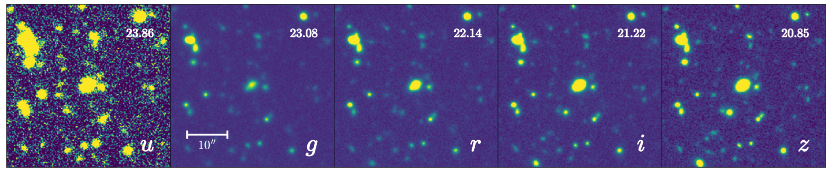
Figure 1: CLAUDS+HSC images of an SFG (centre) with mass $\log M=10.53$ at $z=0.67$ ($\alpha$: 150.17897, $\delta$: 2.03213) in u, g, r, i and z bands. Image cutouts are of dimensions $\sim 33.8^{\prime\prime}\times 33.8^{\prime\prime}$ and have the same intensity stretch. A $10^{\prime\prime}$ ($72.3$ kpc) scale is shown for reference in the middle panel.

CFHT CLAUDS (Sawicki et al., 2019) and Subaru HSC-SSP (Aihara et al., 2018, 2019) surveys together provide the ideal dataset for studies of galaxy morphology in rest-frame UV and visible lights at $z<1$. The CLAUDS+HSC survey includes deep images of the sky over an overlapping area of $18.6$ deg² in $6$ bands ($Ugrizy$) that range from UV to near infrared (IR). In this pilot study, we use a subset of this dataset (the central $\sim 1.6$ deg² region of the COSMOS field) to analyse the SMR and size evolution of $\sim 16000$ SFGs and $\sim 5200$ QGs at $0.1<z<0.9$ in two rest-frame wavelengths: $3000$ Å and $5000$ Å. We will expand the study to the entire survey volume in the followup analysis.

The plan of this paper is as follows. Section 2 provides an overview of CLAUDS+HSC survey, the data and auxiliary data products we use, sample selection and classification of galaxies into SFGs and QGs. In Section 3, we present details of the methodology for 2D galaxy light profile fitting (Section 3.1). In Section 3 we also provide the results of the simulations we perform to estimate the robustness of the fitting pipeline and the systematic uncertainties present in our morphological measurements (Section 3.2). In addition, we describe how we estimate the rest-frame Sérsic parameters in Section 3.3. We validate our size measurements by comparing them with those from the literature (Section 3.4). In Section 4, we describe the analytic fits to the SMR and present the results of SMR fitting and size evolution for SFGs and QGs in two rest-frame wavelengths. We discuss the implications of our findings in Section 5. We summarize the major conclusions based on our analysis in Section 6.

Throughout this study, we use $M$ to denote stellar mass in solar units ($M_{\star}/$M_⊙) unless otherwise stated. Additionally, we use the AB magnitude system and adopt a standard cosmology with $\Omega_{M}=0.3$, $\Omega_{\Lambda}=0.7$ and $h=0.7$ throughout this paper.

2 Data and Sample Selection

2.1 CLAUDS+HSC Survey

We use the ultra deep multi-band ($u+griz$) imaging data from the central $1.6$ deg² region of the COSMOS field from CFHT Large Area $U$-band Deep Survey (CLAUDS; Sawicki et al., 2019) and the Hyper Suprime-Cam Subaru Strategic Program (HSC-SSP; Aihara et al., 2018, 2019). In total, the combined deep CLAUDS+HSC dataset covers an overlapping area of $18.6$ deg². In u and i bands, the median depth is $27.1$ mag (measured at $5\sigma$ level in $2^{\prime\prime}$ apertures). The depth of the dataset is optimal for the analysis of massive galaxy morphology out to their faint outskirts. The CLAUDS+HSC bands also have similar sensitivities, except for y-band where the limiting magnitude is $25.6$ mag. Figure 1 shows an example galaxy from our dataset in u, g, r, i and z bands.

Recently, Kawinwanichakij et al. (2021) conducted an extensive morphological study using HSC-SSP data only (i.e., without the u-band images that are available only for the Deep and UltraDeep layers of the HSC-SSP). The u-band data are important for constraining photometric redshifts and internal galaxy properties. For example, u-band photometry is essential for bracketing the Balmer and $4000$ Å  breaks in order to estimate photometric redshifts (photo-$z$’s) accurately for galaxies at intermediate redshifts ($0<z\lesssim 0.7$, Sawicki et al., 2019). At these intermediate redshifts, u-band data also play a vital role in constraining star formation rates (SFRs) of galaxies. With the addition of u-band data from CLAUDS to the Deep and UltraDeep layer of HSC-SSP, we are able to minimize the contamination when separating SFGs and QGs at $z<1$ and to analyze structural evolution of the two populations in a unique way.

Although our final goal is to analyze the entire $18.6$ deg² of the survey region, we limit this pilot study to the COSMOS/UltraVISTA field, covering $\sim 1.6$ deg² on the sky. We target this smaller area because it is a widely studied survey region in the sky. Choosing a widely studied field is beneficial as we can compare the results of our work with those of previous and parallel studies. This approach ensures quality control of certain steps implemented in this project and enables us to draw scientific conclusions regarding the physical processes driving the observed trends with more certainty. In addition, the COSMOS field is rich in ancillary data, which we utilize in this study for mass and redshift estimates. In the next stages, we will expand the study to the entire CLAUDS+HSC data to improve statistics and analyze the impact of environment on size evolution of galaxies.

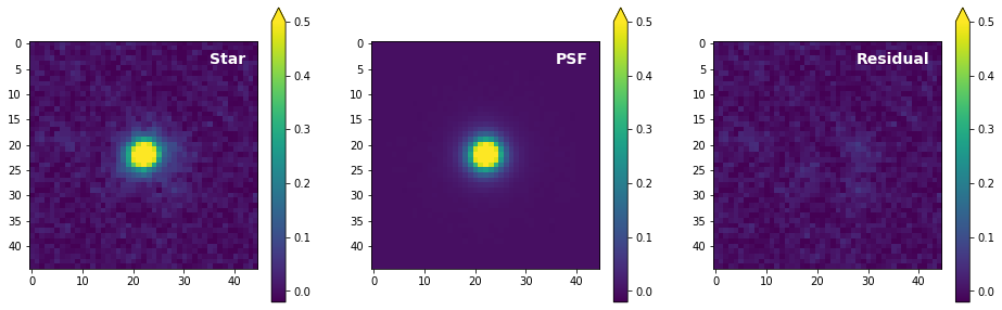
Figure 2: A sample PSF generated for u-band using PSFEx. The left panel shows the image of a star in u-band. The middle panel shows the PSF image generated for the same location in the sky. The last panel shows the residual image obtained by subtracting the PSF from the stellar image.

2.2 Point Spread Function

Atmospheric turbulence (atmospheric seeing) dominates the blurring of astronomical images in ground-based observations. A point spread function (PSF) describes how a point source in the sky (a star) looks like in the image due to this blurring. Hence, to study the intrinsic shapes of galaxies, we must remove the effect of PSF from galaxy images.

The HSC Pipeline uses the PSFEx algorithm (Bertin, 2011) to characterize the PSF of the HSC images. The PSFex adaptation in the HSC Pipeline models PSF from the images of unsaturated stars in an iterative way to remove contamination from neighbouring objects (Bosch et al., 2018). PSF models at any position within the footprint of the survey are available through the PSF picker utility in the Public Data Release by HSC-SSP.

Although PSFs for every sky coordinate covered by the HSC-SSP are available via the PSF picker, fetching a PSF model for every galaxy would be computationally expensive. Hence, we divide every HSC image patch into $36$ sub-regions of dimensions $117.6^{\prime\prime}\times 117.6^{\prime\prime}$. For all galaxies within a sub-region, we use the PSF image at the center of this region.

The PSF images for CLAUDS u-band data are not available externally and thus we model PSFs for these images using PSFEx. Although the software selects the bright unsaturated stars using the catalogue generated by SExtractor, we refine the automated star selection by identifying a region from peak in the surface brightness versus magnitude relation where the unsaturated stars lie. PSEFx then uses these stars to model PSFs for the 36 sub-regions in each image patch.

Figure 2 shows a sample PSF in u-band we generate using PSFEx. The third panel shows the residual after PSF model (second panel) is removed from an image of a star in u-band (first panel). The residual image shows no visible structure, confirming that the u-band PSFs we generated are reliable.

The PSF changes with the band of observations and location in the sky. Among the HSC bands, the i-band has the best seeing with full width at half maximum (FWHM) of the PSF ranges between $0.5^{\prime\prime}$ and $0.7^{\prime\prime}$. The FWHM in u-band is also in the same range. The median FWHM in other bands is $\sim 0.7^{\prime\prime}$.

2.3 Other Data Products

We make use of the COSMOS2020 (Weaver et al., 2022), the latest photometric catalog from Cosmic Evolution Survey (COSMOS, Scoville et al. (2007)). This catalog is based on new imaging and incorporates CFHT CLAUDS u-band data, HSC-SSP PDR2 grizy data, VISTA VIRCAM YJHKs-band data of UltraVISTA DR4 (McCracken et al., 2012) and Spitzer/ IRAC channel $1$, $2$, $3$, and $4$ data of the Cosmic Dawn Survey (Collaboration et al., 2022). The catalogue covers an area of $2$ deg² and includes multiwavelength photometric measurements and derived properties for $1.7$ million sources. From the catalogue, we use the photometric redshifts, stellar masses and star formation rates derived using LePhare (Ilbert et al., 2006) and rest-frame UVJ colours from Eazy code (Brammer et al., 2008).

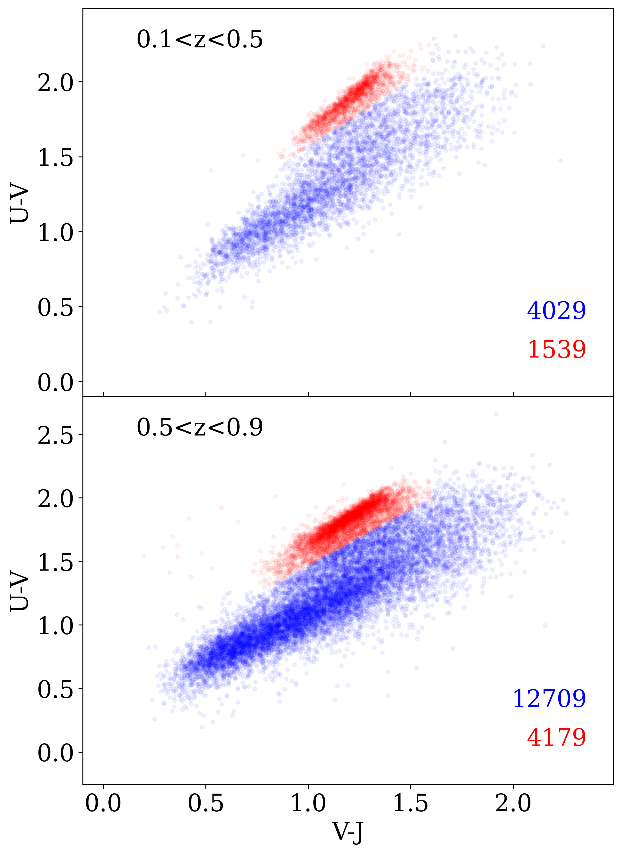
Figure 3: Classification of galaxies into SFGs (blue) and QGs (red) in the UVJ diagram using Equation 1. The upper and lower panels show the classification in two redshift bins. Rest-frame UVJ colours are taken from Weaver et al. (2022).

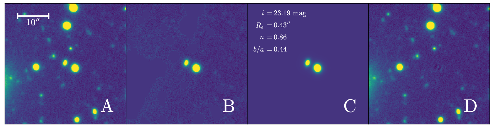
Figure 4: An example of galaxy profile modelling using Galfit. Panels from left to right show the input cutout image of an SFG ($z=0.81$; $\log M=9.56$) in i-band (A), masked image (B), best-fit models (C) and residual image (D). The fitting of the target galaxy (center) is performed simultaneously with a neighbouring bright galaxy on its bottom right. The best-fit parameters of the target galaxy is given in panel D. We also show a $10^{\prime\prime}$ ($77.6$ kpc) scale in panel A for reference.

2.4 Sample Selection and Galaxy Classification

We limit the redshift range of our work to $0.1<z<0.9$ because we cannot constrain the stellar mass of galaxies well beyond $z\sim 0.9$ by using CLAUDS+HSC data alone. This problem arises due to the limitation in the available wavelength coverage to bracket several spectral features like the $4000$ Å  break. Although this pilot study utilises COSMOS2020 catalogue with wider wavelength coverage (Section 2.3), our future studies will cover the complete CLAUDS+HSC deep survey region and thus we will be relying on the data from $Ugrizy$ bands alone.

Furthermore, we select only massive galaxies for this study. The mass completeness limits varies with redshift as well as with the level of galaxy star formation activity. The SFGs at lower redshifts have lower stellar mass completeness limit than the QGs at higher redshifts. To have a uniform mass completeness limit for the entire dataset, we limit our study to galaxies more massive than $\log M>9.5$ (Chen et al. 2024, in prep).

We classify selected galaxies into SFGs and QGs using UVJ colour-colour diagrams (e.g., Wuyts et al., 2007; Williams et al., 2009; Brammer et al., 2011; Muzzin et al., 2013; Carnall et al., 2018) by applying a selection criterion from Whitaker et al. (2011),

$$\begin{split}&(U-V)>0.88\times(V-J)+0.69\ [\mathrm{for}\ z<0.5],\\ &(U-V)>0.88\times(V-J)+0.59\ [\mathrm{for}\ z>0.5],\end{split}$$ (1)

where $U-V$ and $U-J$ are rest-frame colours. Figure 3 shows the UVJ classification of galaxies in two redshift regimes. The sample we analyze in this study contains in total $\sim 16000$ SFGs (blue points) and $\sim 5200$ QGs (red points).

3 Methodology

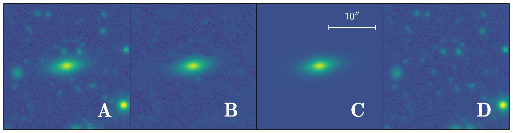
Figure 5: An example for profile modelling of simulated galaxies using Galfit in i-band. The panels are same as in Figure 4 but for a simulated galaxy instead for a real one.

3.1 Galaxy Profile Fitting using Galfit

We model galaxy light profiles with a single Sérsic profile,

$$\log\left(\frac{\Sigma(R)}{\Sigma_{e}}\right)=-b_{n}\left[\left(\frac{R}{R_{e}}\right)^{1/n}-1\right],$$ (2)

where $R_{e}$ is the effective radius, $\Sigma_{e}$ is the surface brightness at $R_{e}$ and $n$ is the Sérsic index, which defines the concentration of the profile. The coefficient $b_{n}$ is not a free parameter; it is a function of $n$ and it ensures that the region within $R_{e}$ encloses half of the total luminosity of the galaxy. Although galaxies usually have several internal components such as disks and bulges, we can fit the overall light profile of a galaxy using a single Sérsic function to obtain its global features (size, light concentration, axis ratio, etc.; van der Wel et al., 2012).

In this work we use Galfit, a two-dimensional ($2$D) parametric light profile fitting software tool to fit galaxy profiles (Peng et al., 2002, 2010a). The software extends the one dimensional Sérsic profile from Equation 2 to $2$D space for direct fitting of galaxy images. Based on the simulations we perform (and describe in Section 3.2), we introduce magnitude cut in each band (u$<26$; g$<25.5$; r, i, z$<25$) that corresponds to $\sim 75\%$ success rate for our fitting pipeline. We do not apply any limit based on other galaxy structural parameters such as size, Séric index or axis ratio, because they do not affect the robustness of our fitting pipeline (see Appendix A). Additionally, we do not fit y-band data because the simulations show that our pipeline does not produce accurate measurements of the structural parameters in that band even for fairly bright galaxies (e.g., $24<y<25$; see Section 3.2.3).

At the start of the fitting procedure, we make an image cutout centred around the target galaxy. We ensure that the size of the cutout is sufficiently large for good fitting by adopting a minimum cutout size of $25\times R_{eS}$, where $R_{eS}$ is the SExtractor effective radius from the COSMOS2020 catalogue (this radius does not take into account the effects of seeing). The cutout size does not exceed $84^{\prime\prime}$. Our simulations (Section 3.2.2) show that the fitting of galaxy profiles using the cutout size of $25\times R_{eS}$ performs significantly better than when using cutout sizes $<20\times R_{eS}$ and that the performance level plateaus around $20-25\times R_{eS}$. Because the HSC PSF images have dimensions of 43 pixels per side, we ensure that the image cutout is at least 45 pixels per side, which is also the dimension of the convolution box for PSF.

We flag neighbouring galaxies for simultaneous fitting if their projected distance from the target galaxy is $<2\times(R_{eS}$(target)$+R_{eS}$(neighbour)$)$, and the magnitude difference is $m_{\text{neighbour}}-m_{\text{target}}<0.5$. If the target galaxy is fainter than the $23$ mag, we further restrict the magnitude range for neighbour selection to ${m_{\text{neighbour}}-m_{\text{target}}<0.1}$.

We then mask out all other fainter galaxies and bright objects in the cutout image. We use a watershed segmentation technique implemented in the Photoutils package for Python for this purpose. The watershed algorithm treats pixel values in the image as an inverted local topography where the centroids of bright objects are at the local minima of this topography. The algorithm generates a segmentation map for the light sources in the image cutout. The algorithm then deblends all overlapping regions and separates the objects in into regions (‘watersheds’). Finally, it creates a file containing pixel coordinates belonging to the ‘watersheds’ of all objects to be masked out.

The next step is to estimate the initial parameters for galaxy fitting. We use magnitudes from COSMOS2020 catalogue as the input magnitude value for Galfit in the respective filters. We roughly estimate the initial values of the other Sérsic parameters (size, Sérsic index, axis ratio) using PetroFit, a galaxy light profile fitting Python package, and provide a random angle for the position angle. We estimate the mean sky background using the areas outside the watershed segments and provide it as the initial parameter. However, if a galaxy is fainter than $24.5$ mag, we fix the sky brightness at this mean sky value while running Galfit. In addition, the software requires $\sigma$-images, that contain the pixel level uncertainties in the data, and the PSF images.

A Galfit Séric model is a fuction of several parameters: centroid pixel coordinates ($x_{0}$, $y_{0}$), magnitude ($m_{tot}$), $R_{e}$, $n$, axis ratio ($b/a$), and position angle ($\theta_{PA}$). We fit galaxy profiles using Galfit in two steps, a procedure similar to the one used by Matharu et al. (2019). In the first step, we keep all parameters free to vary and obtain refined values of galaxy initial position parameters: centroid pixel coordinates ($x_{0}$, $y_{0}$), $b/a$ and $\theta_{PA}$. We provide the best-fit parameters from the first step as the input for the second step, where we force three position parameters to remain constant (within uncertainties) and keep the remaining three structural parameters ($m_{tot}$, $R_{e}$ and $n$) free. We also constrain the parameter space for both steps to ensure that the software reaches global minimum. These constraints are $10\leq m_{tot}\leq 30$, $0.1\leq R_{e}\leq 50$ pix, $0.1\leq n\leq 20$ and $0.02\leq b/a\leq 1$. In addition, we do not allow the Galfit-derived magnitude to differ from the magnitude obtained using SExtractor by more than $2$ mags.

Figure 4 illustrates the steps in fitting of a galaxy light profile. Panel A shows the image cutout, panel B shows the masking using watershed algorithm and panel C the best fit Sérsic models of the target and a neighbouring galaxy. Panel D provides the residual image obtained by subtracting panel C from panel A. From the residual image, it is clear that the fitting pipeline finds Sérsic profile that best matches the observed galaxy (i.e., Panel D shows no features in the region of fitted galaxy). Since we use only a single Sérsic profile for a galaxy, in some cases structural features (such as spiral arms) are visible in the residual image (see the residuals for the neighbouring galaxy in panel D).

3.2 Simulations

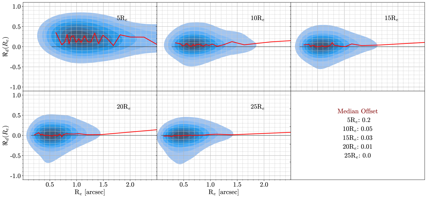
Figure 6: The relative difference in galaxy sizes in i-band from simulations with different cutout sizes. The contours in each panel show the distribution of the relative difference in size: $\Re_{d}=$ (input - output)/input (Equation 3). The red curve in each panel shows the median relative difference in sizes in bins of input galaxy sizes. We perform five sets of simulations, changing the cutout size in relation to the effective radii of simulated galaxies: $5R_{e}$, $10R_{e}$, $15R_{e}$, $20R_{e}$ and $25R_{e}$. In the last panel, we give the median value of the offset in $\Re_{d}(R_{e})$ for each cutout size.

3.2.1 Pipeline

We perform simulations to test the robustness of our galaxy profile fitting procedure (Section 3.1) and to estimate the systematic uncertainties present in the measurements. In these simulations, we generate artificial galaxies and plant them in real images. To ensure that the simulated galaxies reflect the properties of real galaxies, we use the structural parameters of galaxies in the COSMOS field from the Zurich Structure and Morphology Catalogue (ZSMC; Sargent et al., 2007; Scarlata et al., 2007). ZSMC contains Hubble Space Telescope (HST)/ACS F814W-based structural properties of galaxies (Sargent et al., 2007), derived from a single Sérsic profile fitting using GIM2D (Simard, 1998). We first estimate a multivariate probability distribution function (PDF) of GIM2D-derived size ($R_{e}$), Sérsic index ($n$) and axis ratio ($q$) along with u, g, r, i, z and y magnitudes from the CLAUDS+HSC-SSP catalogue (Desprez et al., 2023) using multi-dimensional kernel density estimation. As there are only a few galaxies with $R_{e}>1.5^{\prime\prime}$ in ZSMC, we include additional artificial galaxies with these larger sizes. We then randomly draw parameters from this PDF to simulate galaxy 2D profiles. While doing so, we make sure that we do not draw a parameter set from the multivariate PDF where any of the parameters has a non-physical value (for example, $R_{e}<0$ pixels).

In the next step, we model each artificial galaxy with its randomly chosen parameter set from the PDF using Galfit. We also convolve these artificial galaxies with PSF at the position where we plant them in the image. We then plant these galaxies in real images with randomly chosen position angles ($\theta_{PA}$). Random values of $\theta_{PA}$ ensure that galaxies are placed in the images with orientations similar to those of real galaxies. We also make sure that the centroid of the simulated galaxy does not fall within the effective radius of another real galaxy in the image.

We fit each planted galaxy using the same procedure we use with the real data (Section 3.1). Figure 5 shows an example of a simulated galaxy and its best-fitting model obtained by the pipeline. We perform the planting and fitting procedures using one artificial galaxy at a time to avoid overcrowding of images. One of the caveats of our simulation is that artificial galaxies have single Sérsic profiles, which is not true for most of the real galaxies. Nevertheless, this estimate is sufficient for the present study as we fit real galaxy profiles with a single-profile model.

3.2.2 Cutout image size

Using simulations we first explore the impact of the image cutout size on the fitting results. We perform several sets of simulations with varying cutout sizes based on the size of the target galaxy: $5R_{e}$, $10R_{e}$, $15R_{e}$, $20R_{e}$ and $25R_{e}$.

We define relative difference for a given parameter $x$ as

$$\Re_{d}(x)=\frac{x\,\text{(input)}-x\,\text{(output)}}{x\,\text{(output)}}.$$ (3)

We then analyse the distribution of $\Re_{d}(R_{e})$ as a function of galaxy size in bins of various cutout sizes (Figure 6). Clearly, the smallest cutout size ($5R_{e}$; first panel) performs the worst irrespective of the intrinsic size of the target galaxy. In this case, our pipeline yields sizes that are, based on the median relative difference, $\sim 20\%$ smaller than input values (red line in the first panel of Figure 6). In addition the scatter in relative differences is significantly higher than for any other cutout sizes (blue contours). This error in size measurements is mainly due to two reasons: (1) galaxy profiles are extended beyond $5R_{e}$; (2) there are a few pixels in the cutout to effectively estimate the sky background.

The offset in the size measurements decreases with increasing cutout sizes. With the $25R_{e}$ cutout (last populated panel of Figure 6), the median relative offset (red line) shows that the best-fit $R_{e}$ is equivalent to the real (input) $R_{e}$ irrespective of the input galaxy size. In addition, the scatter in relative galaxy size differences is slightly higher for $20R_{e}$ than for $25R_{e}$ cutout size. Since this scatter represents the systematic uncertainty in galaxy size measurements, we consider a cutout size of $\sim 25R_{e}$ as the best among the five cutout sizes chosen for the simulation and adopt that cutout size for our fitting procedure.

However, unlike simulated galaxies, we do not know the intrinsic sizes of galaxies in real data apriori. Therefore, for real galaxies, we use size estimations from SExtractor to determine the required sizes of image cutouts.

3.2.3 Robustness

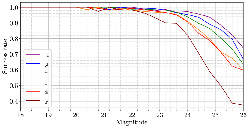
Figure 7: Simulated success rate (Equation 4) as a function of magnitudes in CLAUDS+HSC bands. The u-band data performs the best while the y-band data performs the poorest (see text for details). Hence, we do not use y-band data in this work.

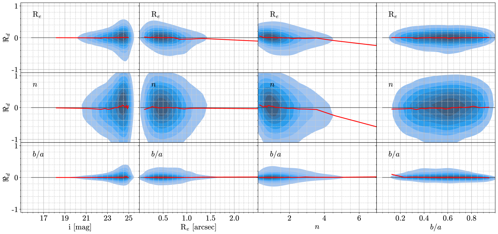
Figure 8: Relative difference in Sérsic parameters in i-band from simulations. The contours in each panel show the distribution of the relative difference in parameters: the top, middle and bottom rows show the relative differences in size, Sérsic index and axis ratios respectively. From left to right, the columns show the relative differences in parameters as functions of Sérsic parameters: magnitude, output size, output Sérsic index and output axis ratio. Note that we have used the relative difference here as $\Re_{d}=$ (input - output)/input (Equation 3). In each panel, the red curve represents the median of the relative difference.

To investigate the robustness of the pipeline, we define the simulated success rate as

$$\text{Success rate}=1-\frac{\text{Number of failures}}{\text{Total number of simulated galaxies}}.$$ (4)

We consider a fit as failed if any of the parameters lies at the limits of the allowed parameter space. We show this ratio in all the six CLAUDS+HSC bands in Figure 7.

We find that the success rate is a function of magnitude in the fitted band with limiting magnitude ranging from $\sim 25$ to $26$ mag for a success rate of $0.75$ in u, g, r, i and z bands. However, we do not find any significant dependence of the success rate on any other Sérsic parameter (see Appendix A). Hence, we limit our analysis based on the magnitude of galaxies in five CLAUDS+HSC bands.

We also note that success rate in the y-band is the lowest among the CLAUDS+HSC bands. It is because the y-band is shallow and has poor seeing compared to other HSC bands. Hence, the fits based on the y-band profiles are more likely to fail for even relatively bright galaxies. Therefore, we do not use galaxy morphology in the y-band for the analysis of galaxy morphological evolution in this work. This does not impact our ability to probe the light profiles of galaxies in two rest-frame wavelengths. For galaxies in our highest redshift bin ($0.75<z<0.9$, Section 4), we use z-band images to model light profiles at the redder rest-frame wavelength ($5000$ Å).

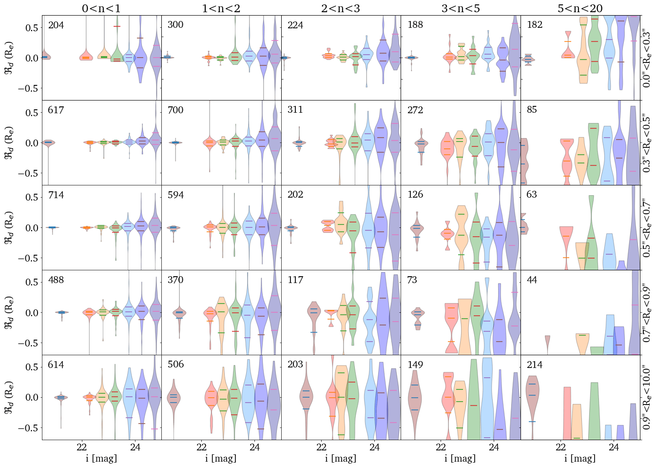
Figure 9: Violin plots showing the distribution of the relative difference in galaxy sizes $\Re_{d}(R_{e})$ in bins of i-band magnitude ($x$-axis), its measured size (rows) and measured Sérsic index (columns). The shape of the violin plots represents the distribution of $\Re_{d}(R_{e})$ in each $3$-D parameter bin, and its $16^{\text{th}}$, $50^{\text{th}}$ and $84^{\text{th}}$ percentiles are shown as horizontal lines. The distributions are approximately Gaussian with their medians around $0$. However, the distributions differ from Gaussian and their median values are significantly different from $0$ for galaxies with higher Sérsic indices or larger sizes that represent the tail of the distribution of galaxy structural properties.

3.2.4 Uncertainty Estimation

An important reason for running these simulations is to estimate the systematic uncertainties in our measurements. To do this, we analyze the distribution of $\Re_{d}(x)$ as a function of magnitude, measured size and measured Sérsic index. The first column of Figure 8 shows $\Re_{d}(x)$ as a function of i-band magnitude. The median relative difference (red curve) in size, Sérsic index or axis ratio does not exhibit any significant systematic offset as a function of magnitude.

If the measured size of a galaxy is large ($R_{e}>0.8^{\prime\prime}$; the first row in the second column of Figure 8), the measurement tends to be slightly larger than the input size. This offset increases with the measured size of the galaxy (offset is above $10\%$ if $R_{e}>1.5^{\prime\prime}$). We also tend to overestimate the Sérsic index of a galaxy if its measured size is greater than $1.5^{\prime\prime}$ (second panel in the middle row). These offsets are not significant, and galaxies with large sizes are extremely rare. The median relative differences in $R_{e}$ and $n$ also show offsets if output Sérsic index is greater than $4$ (red curves in the first and second row of the third column in Figure 8). These high Sérsic index galaxies could have complex formation history and are least likely to be described by a single Sérsic index. Furthermore, the ability of our algorithm to estimate structural parameters do not depend on the $b/a$ of galaxies (third column). Therefore, we do not introduce any offset to measured parameters in this study.

In summary, the simulations show that we are able to recover median values for structural parameters in all bands. We do not find any significant systematic offset between the measured $R_{e}$, $n$ or $b/a$ and their input values irrespective of the brightness, size, Sérsic index and axis ratio for most of our model galaxies ($R_{e}\lesssim 1^{\prime\prime}$ and/or $n\lesssim 4$, Figure 8). The median difference between input and output parameters (red curves) in the simulations is always close to $0$. We also find that the size measurements are more robust than the measurements of Sérsic index, as reflected in the scatters (blue contours) of relative differences of $R_{e}$ and $n$. The scatter in the distribution of $\Re_{d}(R_{e})$ is significantly smaller than the scatter in $\Re_{d}(n)$. Finally, we are able to recover the size of the simulated galaxies even if they are very small ($R_{e}<0.2^{\prime\prime}$).

We incorporate the $\Re_{d}$ scatter ( blue contours in Figure 8) into the measurement uncertainty as systematic uncertainty. We do not estimate the systematic uncertainty in a given parameter as a function of each Sérsic parameter separately due to covariance between them. We instead analyze the scatter in the relative differences in multi-dimensional bins of Sérsic parameters. As we do not find any dependence of the $\Re_{d}$ scatter on the measured axis ratio, we do not include $b/a$ in our uncertainty analysis. The violin plots in Figure 9 show the distribution of $\Re_{d}(R_{e})$ in 3-D bins of $m$, $R_{e}$ and $n$. Except for galaxies with high $R_{e}$ and $n$ ($R_{e}>0.7^{\prime\prime}$ and $n>3$; bottom right panels), the distribution is approximately Gaussian. Hence, we can use the standard deviation (std) of the distributions in Figure 9 as a quantitative measure of the systematic uncertainties. We consider the $x\times\text{std}(\Re_{d}(x))$ to be the systematic uncertainty in the parameter $x$, $\sigma_{sys}(x)$. We then estimate the total uncertainty in a measured parameter to be $\sigma^{2}=\sigma_{sys}^{2}+\sigma_{ran}^{2}$, where $\sigma_{ran}$ is the random uncertainty reported by Galfit for a given galaxy. We note that in most cases the $\sigma_{sys}$ is significantly larger than $\sigma_{ran}$.

3.3 Size Measurements in Two Rest-frame Wavelengths

The goal of this work is to perform morphological analysis of galaxies in two rest-frame wavelengths. We choose rest-frame $3000$ Å (UV light) and $5000$ Å (visible light) because they bracket the $4000$ Å break in galaxy spectrum (Bruzual & Charlot, 2003; Conroy, 2013). Because UV light is dominated by the light from young ($<1$ Gyr) massive stars, this light traces the regions of recent star formation activity in galaxies. In contrast, light from the old ($>1$ Gyr) low mass stars contributes significantly to the visible wavelength region of galaxy spectrum. Since low-mass stars represent the bulk of galaxy stellar mass, the visible light traces closely the stellar mass distribution within galaxies.

Earlier studies generally focus on the rest-frame $5000$ Å that traces the stellar mass distribution in galaxies. Furthermore, though many of the studies have multi-wavelength dataset, they often fit galaxy profiles in a single band alone. They first fit a subset of galaxies in multiple bands and estimate colour gradients (i.e., how galaxy size decreases with increasing wavelength). They then use this colour gradient estimation and correct the size measurements of all galaxies in a selected band to obtain size measurement in any desired rest-frame wavelength (e.g., van der Wel et al., 2014; Kawinwanichakij et al., 2021).

In contrast, we fit the light profiles of all galaxies in five bands and use this multi-band structural information to estimate the Sérsic parameters in two rest-frame wavelength regimes. We first estimate the characteristic redshifts at which effective wavelengths of CLAUDS+HSC bands cover these rest-frame wavelengths. As an example, the rest-frame $5000$ Å  corresponds to the effective (observed) wavelengths of r and i bands for galaxies at the characteristic redshift of $z\sim 0.235$ and $z\sim 0.5422$, respectively.

For a galaxy at redshift $z$, which falls between the characteristic redshifts $z_{a}$ and $z_{b}$ corresponding to bands $a$ and $b$, we estimate the rest-frame Sérsic parameter as

$$x_{\text{RF}}=w_{a}x_{a}+w_{b}x_{b},$$ (5)

where $x_{a}$ and $x_{b}$ are Sérsic parameter measurements in bands $a$ and $b$ respectively. We add weights $w_{a}$ and $w_{b}$ as

$$w_{a}=\left|{\frac{{z-z_{a}}}{{z_{b}-z_{a}}}}\right|\\ \text{and}\\ w_{b}=\left|{\frac{{z-z_{b}}}{{z_{b}-z_{a}}}}\right|.$$ (6)

If a galaxy is missing Sérsic parameter measurement in one of the bands (either $a$ or $b$) due to failed fit or magnitude limit, we use the measurement from the available single band.

3.4 Validation via Comparison with Literature

Figure 10: Comparison between size measurements in our study and those in the literature. Left panels show the comparison with the size measurements by van der Wel et al. (2014, v+14) and the right panels show the comparison with Kawinwanichakij et al. (2021, K+21), both corrected to rest-frame $5000$ Å. We use measurements in r, i and z bands to bracket the rest-frame $5000$ Å depending on the redshift of the galaxy (see Section 3.3). Our size measurements are on $y$-axis and those from the literature are on $x$-axis. The blue line shows the median for SFGs and the maroon line is the median relation for QGs. The shaded region indicate the uncertainties in these median sizes. The black line represents the $1:1$ relation. The lower panels show the relative difference in sizes measured as a function of their measurements in the literature. We estimate the relative difference as $\Re_{d}=(R_{e}$(literature) - $R_{e}$(this work$)/$ $R_{e}$(literature). Similar to the upper panels, the median values with their uncertainties are also shown. There is a good agreement between the measurements in this study and those in the literature.

A number of studies use HST to perform the structural analysis of galaxy light profiles. Since we use ground-based data, our images have (on average) $\sim 5$ times larger PSF than HST images. Hence, it is important to investigate how well our ground-based measurements perform when compared to the measurements based on higher-resolution HST data.

We compare our size measurements with those by van der Wel et al. (2012) based on HST Wide Field Camera 3 (WFC3/IR) images (the two left panels in Figure 10). We perform this comparison on a galaxy-by-galaxy basis because the study by van der Wel et al. (2012) also contains the Sérsic profile measurements of galaxies in the COSMOS field. Following the prescription described in that study, we correct HST size measurements to the constant rest-frame wavelength of $5000$ Å. In our measurements, we use weighted average of the measurements in two bands that are closest to the rest-frame $5000$ Å at a given redshift (Section 3.3).

Equivalent to our fitting approach, the measurements by van der Wel et al. (2012) also come from a single Sérsic profile fitting using Galfit. Because of this similarity in the approaches, a comparison between two size measurements is an independent test of the accuracy of galaxy size measurements based on the ground-based data. A direct comparison on a galaxy-by-galaxy basis shows that the galaxy sizes in our study tend to be on average $\sim 5\%$ larger than the measurements based on HST data for both SFGs and QGs (bottom panel in the first column in Figure 10). The fact that ground-based data have worse PSF than the HST data at least partially contributes to the observed offset. At the same time, our data are more sensitive to the low-surface brightness regions than the HST data and therefore our images better incorporate information from outer regions of galaxies. Since the offset is not very large (within uncertainties of individual measurements) and we do not find any trend in this offset with galaxy size, we infer that the size measurements are robust when obtained from the ground-based data with good seeing.

Kawinwanichakij et al. (2021) use the same ground-based images as we do (HSC-SSP). In the right panel of Figure 10 we compare the two ground-based size measurements, using the size estimates in rest-frame $5000$ Å for the comparison (the only estimates avaiable in Kawinwanichakij et al., 2021). Although in general we find a good agreement between these two size measurements, there is a significant offset at smaller sizes ($R_{e}<0.3^{\prime\prime}$): our size measurements are systematically larger than Kawinwanichakij et al. (2021). The offset increases with decreasing galaxy sizes and it is more prominent for SFGs than QGs.

We speculate that the differences between our size measurements and those of Kawinwanichakij et al. (2021) arise from a number of differences between the two fitting approaches. Kawinwanichakij et al. (2021) use Lenstronomy (Birrer et al., 2015; Birrer & Amara, 2018) whereas we use Galfit. In contrast to their single-band size measurements corrected to the rest-frame, we estimate the rest-frame $5000$ Å sizes by combining multi-band data that correspond to this rest-frame wavelength directly, without any corrections. In addition, compared to their cutout images, we select significantly larger cutout images to model the extended profiles of the galaxies. Our simulations show that a large-fitting region is essential to measuring accurately the overall galaxy sizes (Section 3.2.2).

4 Results

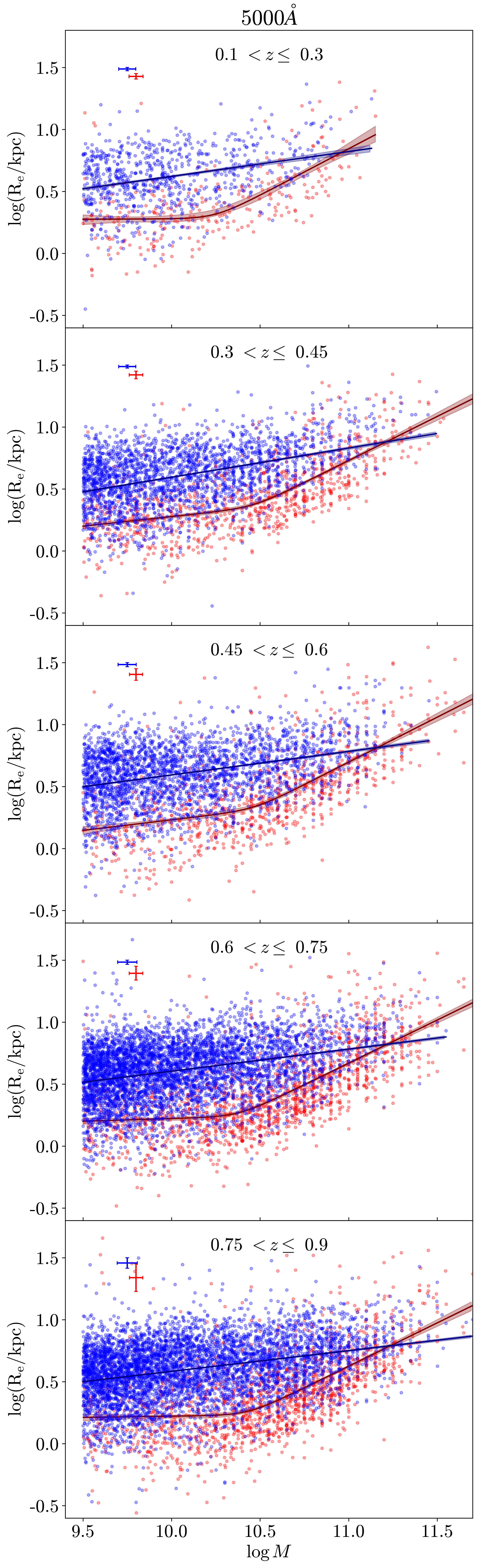
Figure 11: Fitting smoothly broken double power law to the QGs and single power law to the SFGs at rest-frame $5000$ Å in 5 redshift bins. The individual SFGs are shown as blue points; red points represent QGs. The median uncertainties in size measurements for SFGs and QGs are given in the top left corner of each panel. The best-fitting power law relations for SFGs and QGs are shown in navy blue and maroon, respectively, with the uncertainties from Bayesian posterior plotted as shaded region.

cccccccc[hvlines]

1-8Rest-frame $3000$ Å

$z$ median $z$ $\alpha$ $\beta$ $R_{p}$ $\log M_{p}$ $\sigma_{\log{R_{e}}}$ $R_{0}$

$0.1-0.3$ $0.22\pm 0.01$ $0.05\pm 0.14$ $0.61\pm 0.11$ $2.26\pm 0.33$ $10.16\pm 0.17$ $0.21\pm 0.01$ $4.52\pm 0.06$

$0.3-0.45$ $0.35\pm 0.00$ $0.19\pm 0.06$ $0.65\pm 0.08$ $3.27\pm 0.41$ $10.52\pm 0.12$ $0.23\pm 0.01$ $4.07\pm 0.02$

$0.45-0.6$ $0.53\pm 0.00$ $0.20\pm 0.12$ $0.60\pm 0.07$ $3.18\pm 0.56$ $10.52\pm 0.16$ $0.27\pm 0.01$ $3.91\pm 0.03$

$0.6-0.75$ $0.68\pm 0.00$ $0.12\pm 0.08$ $0.71\pm 0.04$ $2.65\pm 0.20$ $10.49\pm 0.07$ $0.26\pm 0.01$ $3.48\pm 0.01$

$0.75-0.9$ $0.83\pm 0.00$ $0.04\pm 0.12$ $0.59\pm 0.06$ $3.35\pm 0.32$ $10.57\pm 0.10$ $0.28\pm 0.01$ $3.82\pm 0.01$

1-8Rest-frame $5000$ Å

$z$ median $z$ $\alpha$ $\beta$ $R_{p}$ $\log M_{p}$ $\sigma_{\log{R_{e}}}$ $R_{0}$

$0.1-0.3$ $0.22\pm 0.01$ $0.01\pm 0.12$ $0.75\pm 0.14$ $2.08\pm 0.28$ $10.25\pm 0.15$ $0.22\pm 0.01$ $4.15\pm 0.05$

$0.3-0.45$ $0.36\pm 0.00$ $0.15\pm 0.04$ $0.71\pm 0.05$ $2.38\pm 0.19$ $10.47\pm 0.07$ $0.21\pm 0.00$ $3.28\pm 0.01$

$0.45-0.6$ $0.53\pm 0.00$ $0.17\pm 0.06$ $0.73\pm 0.05$ $2.18\pm 0.22$ $10.47\pm 0.09$ $0.24\pm 0.01$ $3.02\pm 0.01$

$0.6-0.75$ $0.68\pm 0.00$ $0.04\pm 0.05$ $0.70\pm 0.04$ $1.87\pm 0.12$ $10.38\pm 0.06$ $0.24\pm 0.00$ $2.87\pm 0.01$

$0.75-0.9$ $0.84\pm 0.00$ $0.02\pm 0.06$ $0.70\pm 0.04$ $1.83\pm 0.12$ $10.43\pm 0.07$ $0.26\pm 0.00$ $2.60\pm 0.00$

Table 1: The best-fit parameters of double power law SMR for QGs in two rest-frame wavelengths: $3000$ Å and $5000$ Å (Equation 8). Here $R_{0}$ denotes the characteristic size of QGs at $5\times 10^{10}$M_⊙. Uncertainties smaller than $0.005$ are rounded as $0.00$. Both $R_{p}$ and $R_{0}$ are in kpc and $M_{p}$ is in M_⊙.

cccccc[hvlines]

1-6Rest-frame $3000$ Å

Galaxy $z$ median $z$ $\alpha$ $R_{0}$ $\sigma_{\log{R_{0}}}$

5-1SFGs 0.1-0.3 $0.23\pm 0.00$ $0.22\pm 0.03$ $6.35\pm 0.30$ $0.22\pm 0.01$

0.3-0.45 $0.36\pm 0.00$ $0.28\pm 0.01$ $6.49\pm 0.15$ $0.24\pm 0.00$

0.45-0.6 $0.53\pm 0.00$ $0.22\pm 0.01$ $6.02\pm 0.14$ $0.25\pm 0.00$

0.6-0.75 $0.69\pm 0.00$ $0.20\pm 0.01$ $5.95\pm 0.09$ $0.24\pm 0.00$

0.75-0.9 $0.84\pm 0.00$ $0.19\pm 0.01$ $5.83\pm 0.08$ $0.24\pm 0.00$

5-1QGs 0.1-0.3 $0.23\pm 0.01$ $0.58\pm 0.08$ $4.57\pm 0.23$ $0.20\pm 0.01$

0.3-0.45 $0.37\pm 0.00$ $0.61\pm 0.05$ $4.14\pm 0.13$ $0.21\pm 0.01$

0.45-0.6 $0.53\pm 0.00$ $0.59\pm 0.06$ $3.94\pm 0.17$ $0.25\pm 0.01$

0.6-0.75 $0.69\pm 0.00$ $0.70\pm 0.03$ $3.48\pm 0.09$ $0.25\pm 0.01$

0.75-0.9 $0.84\pm 0.00$ $0.59\pm 0.04$ $3.77\pm 0.13$ $0.26\pm 0.01$

1-6Rest-frame $5000$ Å

Galaxy $z$ median $z$ $\alpha$ $R_{0}$ $\sigma_{\log{R_{0}}}$

5-1SFGs 0.1-0.3 $0.23\pm 0.00$ $0.20\pm 0.02$ $5.76\pm 0.23$ $0.21\pm 0.01$

0.3-0.45 $0.36\pm 0.00$ $0.24\pm 0.01$ $5.74\pm 0.11$ $0.21\pm 0.00$

0.45-0.6 $0.53\pm 0.00$ $0.19\pm 0.01$ $5.32\pm 0.09$ $0.22\pm 0.00$

0.6-0.75 $0.69\pm 0.00$ $0.18\pm 0.01$ $5.35\pm 0.07$ $0.22\pm 0.00$

0.75-0.9 $0.84\pm 0.00$ $0.17\pm 0.01$ $5.01\pm 0.06$ $0.22\pm 0.00$

5-1QGs 0.1-0.3 $0.25\pm 0.01$ $0.73\pm 0.08$ $4.18\pm 0.19$ $0.21\pm 0.01$

0.3-0.45 $0.37\pm 0.00$ $0.67\pm 0.04$ $3.36\pm 0.08$ $0.21\pm 0.01$

0.45-0.6 $0.53\pm 0.00$ $0.69\pm 0.04$ $3.10\pm 0.09$ $0.23\pm 0.01$

0.6-0.75 $0.69\pm 0.00$ $0.68\pm 0.03$ $2.90\pm 0.06$ $0.24\pm 0.01$

0.75-0.9 $0.84\pm 0.00$ $0.67\pm 0.03$ $2.64\pm 0.05$ $0.24\pm 0.01$

Table 2: The best-fitting parameters from the single power law SMR for SFGs and QGs in two rest-frame wavelengths (Equation 7). Uncertainties smaller than $0.005$ are rounded as $0.00$. The unit of $R_{0}$ is in kpc.

4.1 Size-Stellar Mass Relation

Observations show that galaxies exhibit a relation between their stellar mass and size(SMR) at least up to $z\sim 3$ (e.g., Shen et al., 2003; Trujillo et al., 2004; Guo et al., 2009; Williams et al., 2010; Newman et al., 2012; van der Wel et al., 2014; Lange et al., 2015; Faisst et al., 2017; Roy et al., 2018; Mowla et al., 2019b; Matharu et al., 2019, 2020). The form of the SMR differs between the SFGs and QGs (e.g., van der Wel et al., 2014; Mowla et al., 2019b; Kawinwanichakij et al., 2021).

SFGs exhibit a linear relation between galaxy size and stellar mass in log-log space:

$$\log R_{e}=\log R_{0}+\alpha\log\left(\frac{M}{M_{0}}\right),$$ (7)

where $\alpha$ is the slope and $R_{0}$ is the characteristic size at the fiducial mass, $M_{0}$ (e.g., van der Wel et al., 2014; Kawinwanichakij et al., 2021). In line with the literature, we adopt $M_{0}=5\times 10^{10}$M_⊙. Figure 11 illustrates the SMR at rest-frame $5000$ Å for SFGs in our sample divided into five redshift bins (with data points in blue and the best fit relation as blue-shaded line). In Appendix B, we show the SMR for our SFGs at rest-frame $3000$ Å.

However, QGs have a more complex SMR where the slope changes at the pivot mass $\sim 3\times 10^{10}$M_⊙ (Lange et al., 2015; Mowla et al., 2019a; Mosleh et al., 2020; Kawinwanichakij et al., 2021; Nedkova et al., 2021; Damjanov et al., 2023). Hence, to explore the trend in size with stellar mass for QGs, we first fit a smoothly broken double power law,

$$R(M)=R_{p}\left(\frac{M}{M_{p}}\right)^{\alpha}\left[\frac{1}{2}{\left(1+\frac{M}{M_{p}}\right)^{\delta}}\right]^{\frac{\beta-\alpha}{\delta}},$$ (8)

where $M_{p}$ is the pivot stellar mass at which the slope changes, $R_{p}$ is the effective radius at the pivot stellar mass, $\alpha$ is the slope of the SMR at the low-mass end, $\beta$ is the slope at the high-mass end, and $\delta$ is the smoothing factor. Following Mowla et al. (2019a), we adopt $\delta=6$ to reduce degeneracy between $\delta$ and the slopes.

We fit the SMR for both SFGs and QGs using Dynesty, a Python package designed to fit the data by implementing Bayesian inference (Speagle, 2020). We follow the fitting procedure from van der Wel et al. (2014, see their Section 3). The differences between our approach and the method of van der Wel et al. (2014) are the use of the double power law for QGs and how total likelihood is estimated in our study. van der Wel et al. (2014) introduce a $10\%$ contamination in the dataset due to misclassification of SFGs and QGs. Since we use UVJ classification where the separation criteria varies with redshift, we do not account for contamination in this study. Additionally, they also allow for $1\%$ outliers (objects that should not be in the data) in the likelihood estimation.

Our likelihood function is of the form

$$\mathcal{L}=\ln{(wp)},$$ (9)

where $w$ is a weighting factor and $p$ is the probability of observing the given size for a galaxy of mass $M_{*}$ as described by van der Wel et al. (2014, their Equation 4). The weighting factor, $w$, is inversely proportional to the galaxy number density at a given stellar mass taken from the stellar mass functions of Muzzin et al. (2013). By applying this weight, we ensure that each stellar mass range contributes equally to the SMR fit.

We first fit the double power-law to the SMR of QGs. Figure 11 shows (in red) the distribution of galaxies in this parameter space and the best-fit relations in five different redshift bins in the rest-frame $5000$ Å  (see Appendix B for the results in rest-frame $3000$ Å). It is clear that QGs have shallower SMR slopes at stellar masses below the pivot mass compared to those of more massive QGs. The SMR for the low mass QGs is horizontal within $2\sigma$ (i.e., $\alpha\sim 0$). These shallow slopes of low mass QGs ($M<M_{p}$) are also consistent, within their uncertainties, with the results of Kawinwanichakij et al. (2021) and Nedkova et al. (2021). However, the QGs show a steep SMR above the pivot mass, $M_{p}(z)$. This pivot mass is around $\log M\sim 10.5$, except in the lowest redshift bin where it drops to $\sim 10.3$. In addition, the high-mass end slopes $\beta$ do not change significantly across the full redshift interval. Table 4 gives the best fit parameters of the double power law fitting of QGs in two rest-frame wavelengths.

Once we estimate the pivot point, we fit the SMR for the QGs with stellar masses larger than $M_{p}(z)$ and SFGs that are more massive than $10^{9.5}M_{\odot}$ (mass completeness limit; Section 2.4) using the single-power law from Equation 7. We use the Equation 7 for QGs to be able to directly compare our findings with the results from the literature (Section 4.2). This approach captures the nature of SMR for QGs when we limit our analysis to very massive QGs (above the pivot point). The SMR fitting procedure is the same as above. We fit the SMR for SFGs and QGs separately without considering any cross-contamination between the two populations. Unlike van der Wel et al. (2014), we use moving UVJ separation line (with $z$) which further reduces contamination (Whitaker et al., 2011). The best-fit parameters are given in Table 4.

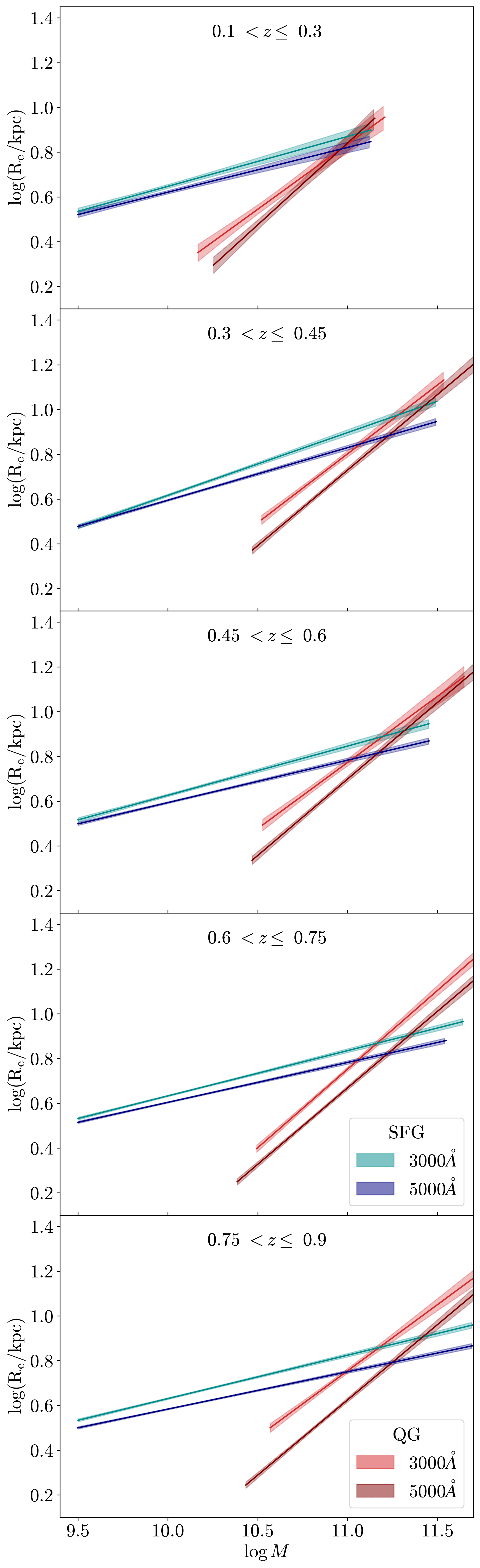
Figure 12: The best-fitting single power-law SMR for SFGs and massive QGs in two rest-frame wavelengths ($3000$ Å and $5000$ Å) in five redshift bins. The shaded regions represent the fit uncertainties estimated from the Bayesian posterior for SFGs and QGs respectively. The SMR fits for SFGs and QGs in the shorter wavelength are plotted in cyan and red, respectively. The fits for SFGs and QGs in the longer wavelengths are shown in navy blue and maroon, respectively.

Figure 12 shows the resulting SMR in the rest-frame $5000$ Å for SFGs and QGs (in navy blue and maroon, respectively) separated into five redshift bins. This figure includes the best-fit SMRs for SFGs from Figure 11. For QGs, the Figure 12 shows the best-fitting single power-law for massive QGs above the pivot point ($M>M_{p}$).

The results are mostly consistent with previous works. Except at very high masses, the sizes of SFGs are larger than those of QGs at a given stellar mass as shown previously by Shen et al. (2003), Williams et al. (2010), van der Wel et al. (2014), Mosleh et al. (2020), Kawinwanichakij et al. (2021) and others. At very high masses ($\log M\gtrsim 11.2$), we find that the average size of QGs becomes comparable to that of SFGs. The slopes of the SMR for SFGs ($\alpha\sim 0.2$) and massive QGs ($\alpha\sim 0.7$) are similar to those in the literature (van der Wel et al., 2014; Mowla et al., 2019b; Kawinwanichakij et al., 2021; Nedkova et al., 2021).

Figure 12 also shows the resulting best-fit SMRs in the rest-frame $3000$ Å for both SFGs and QGs (in cyan and red, respectively; see Figure 28 for the distribution of individual data points in this parameter space). Except for the clear offset in the zero-points, the results in the rest-frame $3000$ Å are also very similar to the results in the rest-frame $5000$ Å. For stellar masses $\log M\lesssim 11.2$, the SFGs are, on average, larger than QGs. The slopes of the SFGs are comparable between the two wavelengths ($\alpha\sim 0.2$). At the same time, the SMR for QGs is systematically $\sim 10\%$ steeper in the red light than in the blue light, although this difference is within $2\sigma$ uncertainty on the slope estimates. We return to the difference in the SMR zero points for two rest-frame wavelengths in Section 4.3.

4.2 Median Size Evolution in the Rest-frame Visible Light

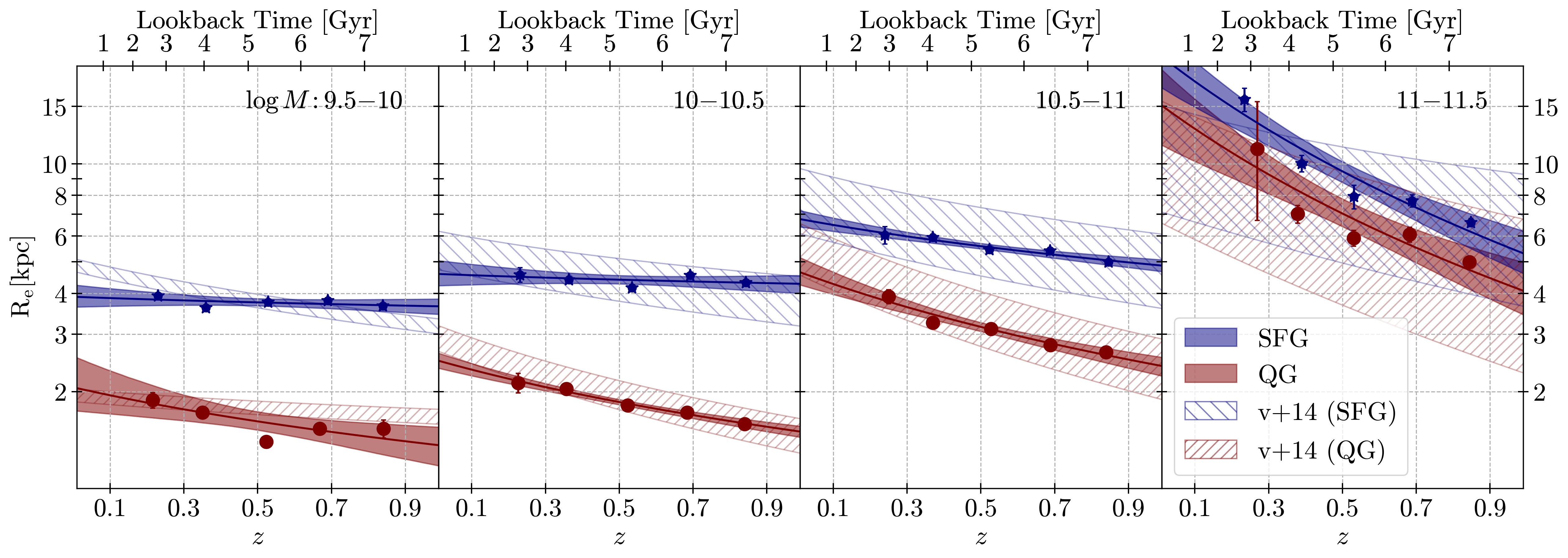
Figure 13: Evolution of the median galaxy sizes at fixed stellar mass in rest-frame $5000$ Å for galaxies segregated in four mass bins. Mass bins are noted in the top right corner of each panel. SFG population is represented by blue colour and the QG population is shown in red. The median sizes in five redshift bins are shown with stars for SFGs and with circles for QGs along with their bootstrapped error bars. The size evolution is represented by a power-law, $A(1+z)^{\beta}$ (solid curves with uncertainties from Bayesian posterior as shaded region). For comparison, we show the results from van der Wel et al. (2014, v+14) as well. Their best fitting evolution curves for SFGs and QGs at rest-frame $5000$ Å are shown in blue and red hatched regions respectively. In general, there is a good agreement between our results and those of v+14.

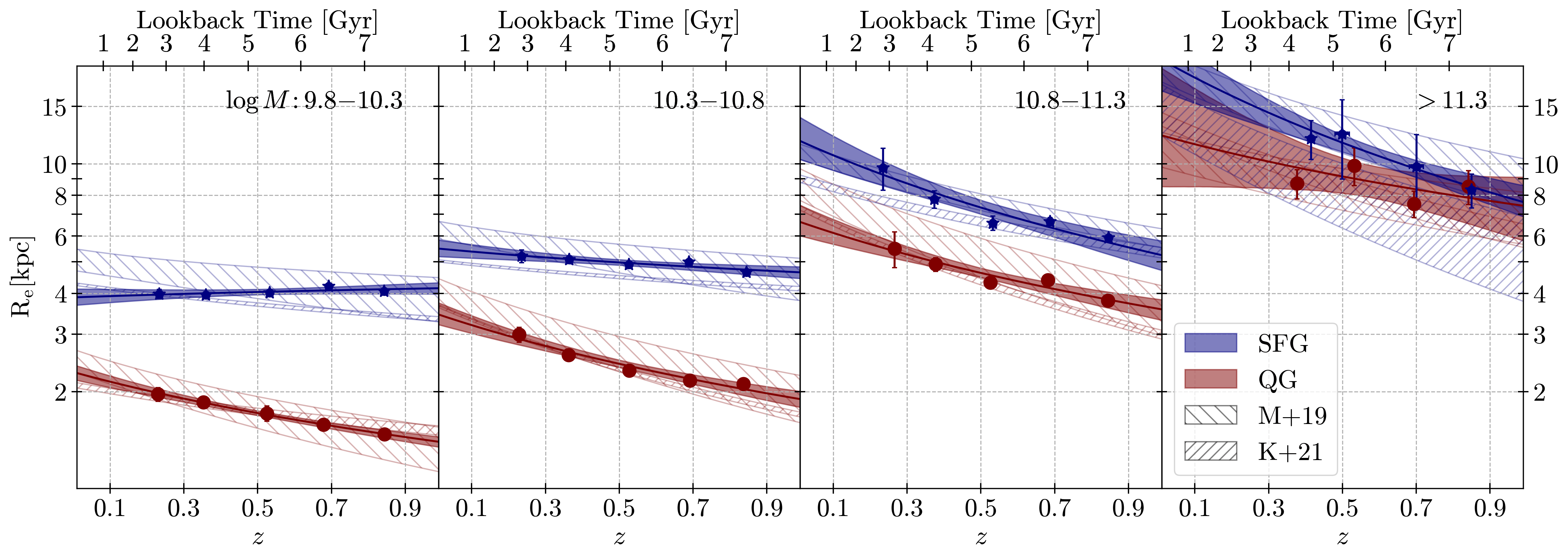
Figure 14: Comparison of the size evolution at fixed stellar mass for SFGs and QGs we trace in four stellar mass bins with the results of Mowla et al. (2019b, M+19) and Kawinwanichakij et al. (2021, K+21). The size evolution reported by M+19 and K+21 are shown as hatched regions. Rest of the details in the figure are the same as in Figure 13. In general, there is a good agreement between our results and the literature.

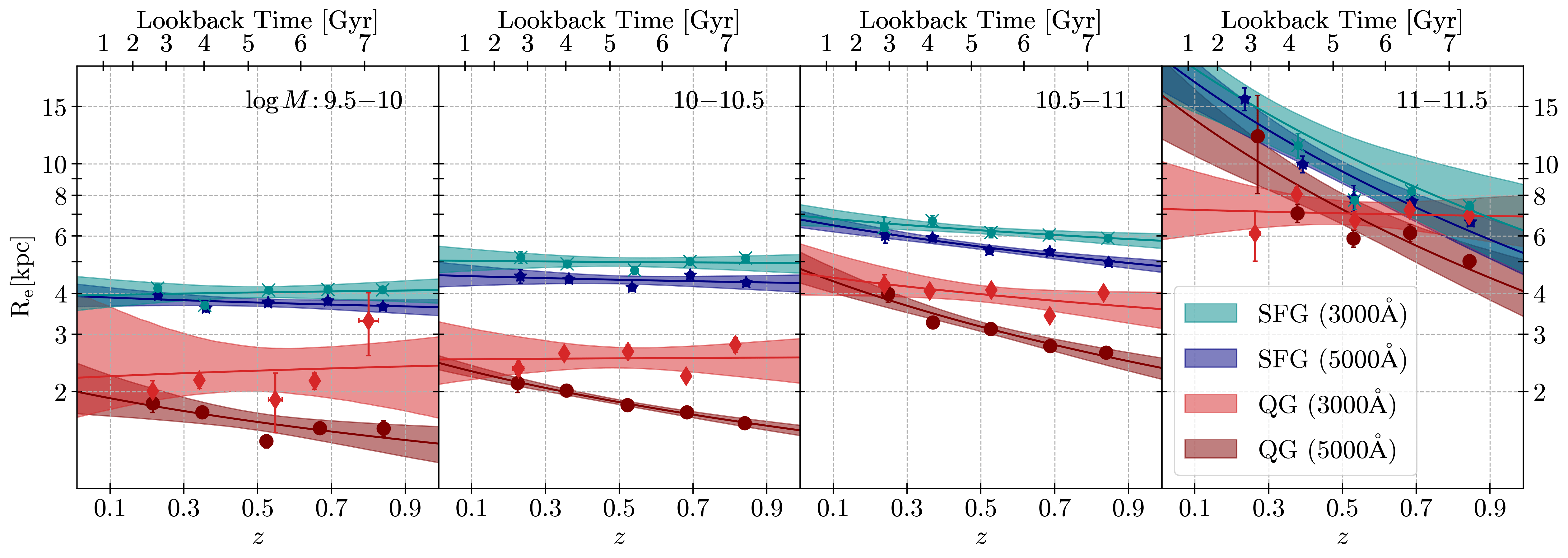
Figure 15: Comparison of the median size evolution for SFGs and QGs at fixed mass between rest-frames UV ($3000$ Å) and visible ($5000$ Å) light. As in Figure 13, panels show the median size evolution in various mass bins as denoted in the top right corner of each panel. Cyan and navy blue represent SFG population in rest-frames $3000$ Å and $5000$ Å respectively. Similarly, red and maroon colours denote QG population in rest-frame $3000$ Å and $5000$ Å respectively. The best fitting power-law functions (solid curves) for the size evolution of SFGs and QGs are shown with their uncertainties (shaded regions). Galaxies are more extended in shorter wavelength than in longer wavelength.

We further employ galaxy size measurements to explore the trend in median size with redshift for SFGs and QGs segregated by stellar mass. First, we use median galaxy sizes to explore galaxy size evolution in the rest-frame wavelength of $5000$ Å.

Figure 13 shows the median sizes of SFGs and QGs in this rest-frame wavelength as a function of redshift in four different stellar mass bins. Within each bin, the stellar mass range is fixed across the full redshift interval. In addition to SFGs having larger sizes than QGs, median sizes of both galaxy populations at a given fixed stellar mass generally grow with cosmic time.

We fit the redshift evolution in size of SFGs and QGs with a power law,

$$R_{e}=R_{e}^{0}(1+z)^{\beta},$$ (10)

where $R_{e}^{0}$ is $R_{e}$ at $z=0$. When traced in the rest-frame visible light, the pace of size evolution differs between SFGs and QGs (blue vs. red solid lines in Figure 13). In all mass bins below $\log M\sim 11$, sizes of QGs evolve faster than those of SFGs. In the mass range $10.5<\log M<11$ and over the redshift interval $0.1<z<0.9$, the median sizes of QGs grow as $R_{e}\varpropto(1+z)^{-1.0}$ whereas the sizes of SFGs grow as $R_{e}\varpropto(1+z)^{-0.5}$. For example, the average sizes of $\log M\sim 10.75$ QGs grow by $\sim 73\%$ in the time interval of 6.1 Gyrs. In contrast, similarly massive SFG grows in size by only $\sim 31\%$ over the same time interval.

Furthermore, for both galaxy populations, the pace at which galaxies grow is faster for more massive systems. The growth rate $\beta=\frac{d\log{(R_{e}/\mathrm{kpc})}}{d\log(1+z)}$ for SFGs ranges from $0.10\pm 0.18$ for the least massive to $-2.07\pm 0.45$ for the most massive SFGs (blue lines in Figure 13). Over the same mass range, the growth rate for QGs changes from $\beta=-0.55\pm 0.4$ to $\beta=-1.94\pm 0.64$ (red lines in Figure 13). QGs grow significantly in size at $z<1$ even at lower masses ($\log M<10.5$). In contrast, the size evolution of SFGs at these low masses is, within uncertainties, consistent with no growth.

We note that these growth rates are the median trends for galaxy populations, not individual galaxies. Furthermore, for now we do not consider the fact that stellar mass of SFGs also grows through star formation. Finally, here we do not account for the effect of progenitor bias among QG population. We estimate the amplitude of the effects that mass growth and progenitor bias have on the evolution in average size of SFGs and QGs in Section 5.

Our findings are in good agreement with results reported in the literature. In Figure 13, we compare our results (solid curves and shaded regions) with those from van der Wel et al. (2014, hatched region) at rest-frame $5000$ Å. Like us, they have fitted galaxy images using Galfit. However, their fits are based on galaxy images taken with WFC3 onboard HST, which has at least 4 times better resolution than our ground-based HSC images (see Section 3.4). Furthermore, we note that their best-fitting relation between median size and redshift spans the redshift interval $0<z<3$. Finally, they only have two redshift bins at $z<1$ while we have a finer sampling of this redshift range with $5$ bins. Despite these differences, we find an excellent agreement between our trends and results reported in van der Wel et al. (2014).

In Figure 14 we compare our results (solid lines with shaded regions) with Mowla et al. (2019b, backward hatched regions) and Kawinwanichakij et al. (2021, forward hatched regions). Mowla et al. (2019b) follow a similar methodology as ours: they fit the galaxy light profiles using Galfit. However, their measurements are based on the same HST imaging as the ones reported in van der Wel et al. (2014) and thus do not suffer from atmospheric seeing effects. Furthermore, they measure galaxy size growth over the redshift interval $0<z<3$, with only two redshift bins below $z\sim 1$. At the same time, Kawinwanichakij et al. (2021) use a ground-based HSC dataset similar to ours, but follow a different methodology (see Section 3.4 for details).

Except for the marginal difference for SFGs in the lowest mass bin (first panel of Figure 14), the agreement between our results and the results of Mowla et al. (2019b) is excellent. With our dataset that covers larger area of the COSMOS field (Section 2.1), we are able to obtain a narrower confidence interval (shaded regions in Figure 14).

In general, our median size evolution estimates for QGs are in agreement with Kawinwanichakij et al. (2021), but we do find some discrepancy between the measurements for SFGs. Overall, the median SFG size measurements of Kawinwanichakij et al. (2021, blue forward hatched regions in Figure 14) are smaller than our measurements and those of Mowla et al. (2019b). This offset could could be a combination of several effects. As we discuss in Section 3.4, the two ground-based studies (this study and that of Kawinwanichakij et al. (2021)) use different methodology to fit galaxy light profiles. In addition, we select significantly larger cutout images to model the extended galaxy profiles. Furthermore, we have much better estimation of photo-$z$’s and UVJ based SFG-QG classification thanks to $U+grizy+JHK$ data from COSMOS2020, whilst Kawinwanichakij et al. (2021) use only HSC $grizy$ data to segregate galaxies into SFGs and QGs. On the other hand, our study is somewhat affected by cosmic variance because our dataset covers almost two orders of magnitude smaller area on the sky (1.6 deg² of the COSMOS field vs $100$ deg² of the HSC-SSP analyzed in Kawinwanichakij et al. 2021). Using the Equation $3$ from Driver & Robotham (2010), we estimate that the cosmic variance will decrease by a factor of $4$ when we expand to the full CLAUDS+HSC survey area (from $12\%$ to $3\%$).

The slower pace of evolution for SFGs compared to QGs for galaxies with $\log M<11$ in the rest-frame $5000$ Å is consistent with the suite of previous studies (e.g., Lilly et al., 1998; Ravindranath et al., 2004; Barden et al., 2005; van der Wel et al., 2014; Mowla et al., 2019b; Kawinwanichakij et al., 2021). Additionally, similar to our findings, van der Wel et al. (2014), Mowla et al. (2019b) and Kawinwanichakij et al. (2021) find that the rate of median size evolution for both QGs and SFGs depends on galaxy stellar mass. This comparison confirms that the resolution of the HSC+CLAUDS imaging dataset is well suited for detailed probes of galaxy size evolution up to $z\sim 1$.

4.3 Median Size Evolution in Rest-frame UV Light

In addition to the rest-frame visible light, we also investigate the size evolution of galaxies in rest-frame UV ($3000$ Å). The comparison of galaxy sizes in two rest-frame wavelengths using a large dataset is unique to our work. These two rest-frame wavelengths ($3000$ and $5000$ Å) represent light coming from young and old stars (see Section 3.3). Hence, comparisons of galaxy morphology in these two rest-frame wavelengths can advance our understanding of the connection between galaxy structural change (i.e., size growth) and the evolution in their stellar content.

We combine the median evolutionary trends in galaxy size at fixed stellar mass in rest-frame UV and visible light for both SFGs and QGs in Figure 15. The median sizes of SFGs and QGs in UV are represented by cyan crosses and red diamonds respectively and those in visible light are in blue stars and maroon circles. We also show the best-fit size evolution trends (solid curves) along with uncertainties (shaded area).

On average, we find that the two galaxy popoulations are larger in rest-frame $3000$ Å  than in $5000$ Å. For example, the median size of SFGs with stellar mass $\log M\sim 10.5$ at $z\sim 0.5$ is $12\%$ larger in rest-frame blue light than in red light (cyan and blue curves in the second panel of Figure 15). The sizes of QGs display even larger difference when measured in two rest-frame wavelengths. At the same mass and redshift ($\log M\sim 10.5$, $z\sim 0.5$) QGs are, on average, $33\%$ more extended in the observations at shorter rest-frame wavelength ($3000$ Å) than in $5000$ Å (red and maroon curves in the second panel of Figure 15).

Several evolutionary trends in galaxy size at the rest-frame wavelegth of $3000$ Å are similar to those we observe at the rest-frame wavelength of $5000$ Å. Firstly, the median UV-based sizes of both SFGs and QGs evolve with cosmic time. At stellar mass range of $10.8<\log M<11$, the median UV-based sizes of SFGs grow by $\sim 50\%$ over the span of $\sim 6.1$ Gyrs ($z=0.9$ to $z=0.1$) whilst sizes of similarly massive QGs grow by $21\%$ in the same rest-frame regime and during the same cosmic period. However, the pace of evolution in rest-frame $3000$ Å is slower than in $5000$ Å. For comparison, in the rest-frame visible light SFGs of similar mass grow by $90\%$ over the same redshift interval; based on their visible light profiles, similarly massive QGs grow by $78\%$ since $z\sim 0.9$.

Finally, the trend in the pace of size evolution with galaxy mass in the rest-frame $3000$ Å is similar to the trend we observe at $5000$ Å except for QGs in the most massive bin ($\log M>11$). SFGs in the most massive bin grow by $\sim 165\%$ whilst at lowest mass bin we do not find any significant evidence for size evolution of either SFG or QG population. However, unlike the rest-frame visible light, the most massive QGs in rest-frame UV do not show any significant signs of growth in median size since $z\sim 1$. Nevertheless, we note that our sample size is small at these higher mass end and the uncertainties are large.

cccc[hvlines]

1-4Rest-frame $3000$ Å

Galaxy $\log M$ $R_{e}^{0}$ $\beta$

4-1SFGs $9.7$ $3.62\pm 0.39$ $0.03\pm 0.24$

$10.2$ $4.95\pm 0.27$ $-0.11\pm 0.12$

$10.7$ $6.83\pm 0.40$ $-0.26\pm 0.13$

$11.2$ $9.57\pm 1.17$ $-0.45\pm 0.27$

2-1QGs $10.7$ $5.06\pm 0.64$ $-0.59\pm 0.28$

$11.2$ $9.68\pm 0.58$ $-0.44\pm 0.14$

1-4Rest-frame $5000$ Å

Galaxy $\log M$ $R_{e}^{0}$ $\beta$

4-1SFGs $9.7$ $3.59\pm 0.30$ $-0.08\pm 0.19$

$10.2$ $4.75\pm 0.28$ $-0.21\pm 0.13$

$10.7$ $6.28\pm 0.38$ $-0.35\pm 0.14$

$11.2$ $8.37\pm 0.76$ $-0.50\pm 0.20$

2-1QGs $10.7$ $5.07\pm 0.58$ $-1.10\pm 0.26$

$11.2$ $11.95\pm 1.96$ $-1.24\pm 0.36$

Table 3: The best-fit parameters for the redshift evolution of characteristic sizes at fixed stellar mass for SFGs and QGs in two rest-frame wavelengths ($R_{e}=R_{e}^{0}(1+z)^{\beta}$). The best-fit curves are displayed in Figures 16 and 21 for SFGs and QGs respectively.

cccc[hvlines]

1-4SFGs

Restframe $\lambda$ $\log M_{(z=0.9)}$ $R_{e}^{0}$ $\beta$

4-1$3000$ Å $9.7$ $7.00\pm 0.44$ $-0.91\pm 0.14$

$10.2$ $8.06\pm 0.63$ $-0.81\pm 0.17$

$10.7$ $9.72\pm 1.15$ $-0.78\pm 0.27$

$11.2$ $12.21\pm 2.03$ $-0.80\pm 0.37$

4-1$5000$ Å $9.7$ $6.42\pm 0.45$ $-0.91\pm 0.16$

$10.2$ $7.25\pm 0.55$ $-0.82\pm 0.17$

$10.7$ $8.52\pm 0.80$ $-0.79\pm 0.21$

$11.2$ $10.37\pm 1.27$ $-0.82\pm 0.28$

Table 4: The best-fit parameters of redshift evolution of characteristic sizes of SFGs with evolving mass as described in Section 5.1.2. The corresponding evolutionary curves are displayed in Figure 17.

5 Discussion

So far we have used the median sizes in several mass bin to trace the size evolution of galaxies in our dataset. Although this approach provides direct comparison with the results based on median size measurements from other studies, it does not formally take into account the uncertainties present in the individual size and mass measurements. At the same time, the SMR fitting procedure incorporates these measurement uncertainties and applies weighting based on galaxy stellar mass functions (Section 4.1). Therefore, we decide to use the size estimates from the best-fitting SMRs for the interpretation of our results. Our conclusions remain the same when we replace the estimates from the best-fit SMRs with the measured median sizes in bins of galaxy stellar mass.

In addition, we also compare this size evolution in two rest-frame wavelengths: $3000$ Å  and $5000$ Å. The analysis of the size growth in two rest-frame wavelengths enables us to trace the distribution of young and old stellar populations in galaxies. We list the parameters of the best-fit function for the redshift evolution of SFG and QG sizes in both wavelengths in Table 4.3.

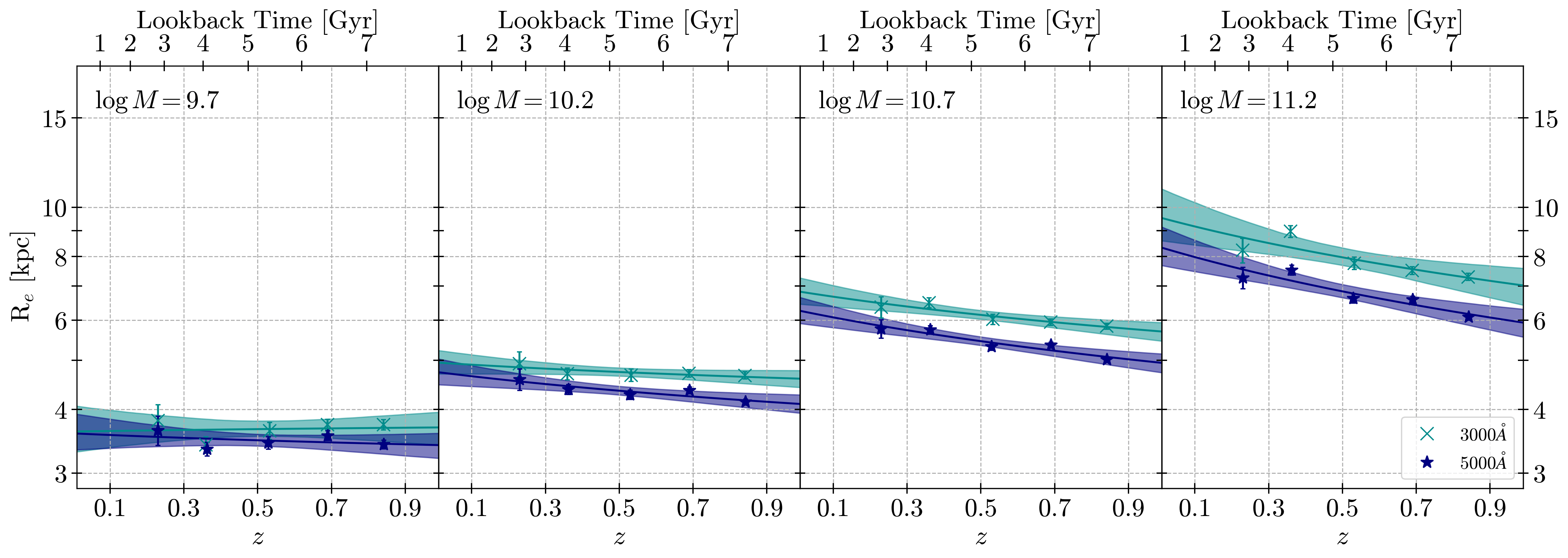
Figure 16: Evolution of characteristic sizes of SFGs at a given fixed stellar mass. Panels show the size evolution of SFGs for a range of characteristic masses (as labeled). The SFG sizes at rest-frame $5000$ Å  are shown in navy blue and at rest-frame $3000$ Å  in cyan. The sizes at shorter wavelength are larger than those at longer wavelengths. The size evolution is fit by a power-law $R_{e}=R_{e}^{0}(1+z)^{\beta}$, and the best fitting parameters are given in Table 4.3. The solid curves show the evolutionary trends as described by these power-law functions with shaded regions showing the $1\sigma$ confidence intervals.

5.1 Size Evolution of Star-Forming Galaxies

5.1.1 Overview of the Observed Trends

Figure 16 shows the size evolution of SFGs in two rest-frame wavelengths for four fixed characteristic stellar masses since $z\sim 1$. As expected, for the evolution in rest-frame $5000$ Å (visible light, navy blue symbols and solid lines with shaded area in Figure 16) we find similar trends as in Section 4.2. The size growth of SFGs is mass dependent: the higher the mass of SFGs, the faster they grow in size with cosmic time. At $\log M=9.7$, SFGs grow only $\sim 5\%$ in size but at $\log M=11.2$, they grow by $31\%$ in $6$ Gyrs from $z\sim 0.9$ to $z\sim 0.1$.

At the characteristic mass of $5\times 10^{10}\text{M}_{\odot}$, van der Wel et al. (2014) report the power-law fit (Equation 10) to the size evolution of SFGs with $\beta=-0.75$ whereas we find $\beta=-0.35\pm 0.14$. When probing the trends in near-IR-based size with redshift for $\log M>10.8$ galaxies Williams et al. (2010) also find a steeper size evolution for SFGs ($\beta=-0.77\pm 0.08$). We note that both Williams et al. (2010) and van der Wel et al. (2014) studies cover wider redshift ranges: $0.5<z<2$ and $0<z<3$ respectively. Thus, their observed evolution is affected by SFGs at $z>1$. Furthermore, the flatter distribution of median SFG sizes below $z\sim 1$ from Figure 4 of Williams et al. (2010) and the agreement between our size measurements and those of van der Wel et al. (2014) suggest that the size evolution of SFGs weakens at $z<1$. Moreover, Oesch et al. (2010) and Mosleh et al. (2012) report faster evolution of SFG sizes at $z>2$. At the same time, studies that focus at $z<1$ (e.g., Lilly et al., 1998; Ravindranath et al., 2004; Barden et al., 2005; Kawinwanichakij et al., 2021) report either a slow or no evolution of the average size of SFGs. Thus, our analysis confirms that the size evolution of SFGs slows down with decreasing redshift and that this change in pace occurs at $z\sim 1$.

As in Figure 15, Figure 16 also includes the size evolution of SFGs in the rest-frame $3000$ Å (cyan symbols and solid lines with shaded area). In general, we find that the sizes of SFGs are larger at shorter wavelength than at the longer one, as we indicate in Section 4.3. For example, at $z=0.5$, SFGs appear $\sim 5\%-17\%$ larger in rest-frame UV than in visible light depending on their stellar mass. Since the shorter wavelength probes the distribution of younger stellar population, the larger size in $3000$ Å  may imply extended (less concentrated) star-forming regions in those star-forming systems. A smaller size at longer wavelength suggests that the older population is more centrally concentrated, in line with the inside-out quenching scenario (Tacchella et al., 2015, 2018; Lin et al., 2019).

The difference between the two rest-frame wavelengths also depends on galaxy stellar mass. The sizes of SFGs at low mass ($\log M<10$) are almost the same at both wavelengths, and the differences in the sizes between the wavelength regimes increase with their stellar mass. At $z=0.5$, an average SFG with stellar mass $\log M=9.7$ has very similar size (within uncertainties) in both red and blue light. However, a massive SFG ($\log M=11.2$) is $\sim 17\%$ larger in blue than in red light.

We interpret the lack of difference in two rest-frame sizes of low-mass SFGs as a sign that low-mass galaxies tend to have their younger and older stars well mixed within their light profiles, without any strong signals of either inside-out or outside-in quenching. However, as the galaxies grow in mass and size, the bulges also grow in the centres of these galaxies. These bulges may eventually suppress star formation by stabilizing the gas within them (e.g., Martig et al., 2009; Saintonge et al., 2012; Sachdeva et al., 2017; Hashemizadeh et al., 2022). As the star formation ceases in the centre, the peak of star formation activity moves to the outskirts of disks. Thus, the massive SFGs tend to look bigger in rest-frame UV than in visible light.

At fixed stellar mass, we find that the pace of SFG size evolution is slightly slower at $3000$ Å than at $5000$ Å. For example, at $\log M=10.7$, SFGs grow by $21\%$ ($\beta=-0.35$) in red light and by $15\%$ ($\beta=-0.26$) in blue light between $z\sim 0.9$ and $z\sim 0.1$. The direction towards faster growth in red light is systematic across all stellar masses of SFGs, but we also note that, within uncertainty, this difference is consistent with the same pace of size evolution in two rest-frame wavelengths.

The slower pace of evolution in blue light than in red light could also indicate the role of bulge growth in the evolution of SFGs. Bulges become more and more significant in the overall galaxy light profile with time (e.g., Sachdeva et al., 2017). As the bulges grow, this growth is reflected in the size evolution of SFGs at longer wavelength where we see a slightly faster pace of size evolution.

There are two scenarios for bulge growth that we can consider: (1) both the bulge and the disk grow in SFGs, and (2) bulge grows into the disk and pushes the peak star-forming regions we can observe at $3000$ Å further out. In the first scenario, the slightly faster pace of SFG size evolution in longer wavelength probing older stellar population could suggest that the growth of bulges is faster than the growth of disks at this redshift range. In the second scenario, since only bulges grow significantly, the size growth in visible light is faster as well. Although pushing the peak star forming regions outward will make the sizes in UV bigger, growth in visible light is still stronger because it encompasses the light from stars in both the growing bulge and the disk. However, we note that we only fit a single Sérsic profile to observed galaxy light profiles. We will explore the two scenarios in more detail in the follow-up study by performing bulge$+$disk decomposition.

Figure 17: Evolution of characteristic sizes of SFGs assuming evolving stellar mass we calculate based on Equation 12 at $z<1$. Each panel shows the size evolution for a galaxy that has labeled stellar mass at $z\sim 0.9$. This characteristic mass then evolves along the redshift space in each panel via in-situ star formation. We adopt the SFR values of star formation main sequence from Speagle et al. (2014) to estimate this stellar mass growth. We then adopt galaxy size considering increased mass and observed SMR at each subsequent redshift point. As in Figure 16, the navy blue stars denote the size in rest-frame $5000$ Å  and the cyan crosses denote those in rest-frame $3000$ Å, along with their bootstrapped error bars. The best fitting power-laws with their uncertainties are represented by solid curves and shaded areas. The parameters of the best-fit power-laws are given in Table 4.3. By selecting galaxies with increased stellar mass at lower redshifts we attempt to analyze the size evolution of SFGs by connecting progenitors to their descendants.

5.1.2 The Effects of SFG Mass Growth

The earlier studies in general look at the galaxy size evolution at a constant stellar mass across the redshift range that they probe (e.g., van der Wel et al., 2014; Mowla et al., 2019b; Kawinwanichakij et al., 2021, and many others). So far, we have also analyzed the size evolution in this manner. However, SFGs are actively forming stars and growing in both size and mass with cosmic time. To study the true size evolution of SFGs, it is important to consider their mass growth.

We use a toy model to trace the size evolution of galaxies having progenitors with similar mass at $z\sim 0.9$ by incorporating mass growth via star-formation. We assume that the SFGs remain on the star-forming main sequence since $z\sim 1$ and that the mass growth is only due to in situ star formation in galaxies. Although galaxies quench and leave the SFG population over cosmic time interval we probe, in the toy model we also assume that this quenching is random and does not affect any sub-population of SFGs specifically.

We adopt the star-forming main sequence relation from Speagle et al. (2014),

$$\log\mathrm{SFR}(M,t)=(0.84-0.026t)\log M+0.11t-6.51,$$ (11)

where $t$ is the age of the universe in Gyr and SFR is in $\hbox{M${}_{\odot}$}/$yr. For SFGs with a specific mass at $z=0.9$, we estimate their mass at various cosmic times between $z=0.9$ and $z=0.1$ as

$$M(t_{2})=M(t_{1})+\int_{t_{1}}^{t_{2}}10^{\log\mathrm{SFR}(M,t)}dt,$$ (12)

where $t_{1}$ is the age of the Universe at $z=0.9$ and $t_{2}$ is its age at the target redshift. We then estimate the characteristic sizes of these SFGs at lower redshifts by taking their increased stellar mass as the input for the SMR (Equation 7) with redshift-dependent parameters from Table 4. Finally, we fit the size evolution of SFGs growing both in mass and size at two different rest-frame wavelengths. Figure 17 illustrates the results and Table 4.3 lists the best-fit parameters of the evolutionary trends for the SFGs with growing stellar mass.

When considering stellar mass growth, for every initial stellar mass (i.e., stellar mass at $z=0.9$) we find that the size growth is faster than the growth at constant mass. In rest-frame visible light, SFGs with initial stellar mass of $\log M=9.7$ grow in size by $\sim 65\%$ when we consider mass growth (navy blue curve in the first panel of Figure 17) against only $\sim 5\%$ growth when the mass growth is ignored in the redshift range we probe (navy blue curve in the first panel of Figure 16). The observed weak/no evolution at the lowest mass bin in Figure 16 ($\beta=-0.08\pm 0.19$ in $5000$ Å) seems to be due to the selection of different galaxies at different redshifts.

At the same time, the SFGs with initial stellar mass $\log M=11.2$ grow in size by $\sim 55\%$ and $\sim 32\%$ with and without stellar mass growth, respectively (last panels in Figures 17 and 16). Thus the difference in size growth with or without simultaneous stellar mass growth decreases with stellar mass. The difference we observe demonstrates that the size evolution of individual galaxies is faster than what is being suggested in the literature because size growth of SFGs cannot be separated from the increase in their stellar mass.

Additionally, we do not find any differential size evolution with stellar mass when we consider mass growth. Our analysis shows that the sizes of all massive SFGs ($\log M>9.5$) grow, within uncertainties, at a constant pace ($\beta\sim-0.8$ to $-0.9$) (Figure 17 and Table 4.3).

Furthermore, the differences in the rate of size growth between two wavelength regimes that we report in Section 5.1.1 disappear when we include stellar mass growth. Both cyan and navy blue curves represent power-law functions with very similar exponents in all panels of Figure 17. However, throughout the redshift range we probe, the SFGs remain more extended in the shorter wavelength than in the longer wavelength in all initial stellar mass bins.

5.1.3 Slowing down of Size Evolution for SFGs

In combination with the observed rates of size growth at $z>1$ from the literature, our results for the star-forming population point to slowing down of SFG size evolution with cosmic time (5.1.1). To explore this further, we separate SFGs into two groups based on $U-V$ colour: red SFGs ($U-V>1$) and blue SFGs ($U-V\leq 1$). In Figure 18 we show the characteristics of these two populations in size-stellar mass parameter space for sizes measured at the rest-frame $5000$ Å. The figure shows that (1) blue SFGs (blue squares) cover a smaller range of masses (up to $10^{10.5}$M_⊙) than red SFGs (purple diamonds); (2) at the same stellar mass, blue SFGs are around $20\%$ larger than red SFGs.

The lack of massive blue SFGs may be related to the extent of the star formation episodes. Blue SFGs are forming stars at high rates and thus are still "catching up" with the SFGs that are in slightly more advanced stage of the evolution (but still on the main sequence). As the SFGs evolve, they become redder in colour because low-mass stars become dominant light source. A fraction of these stars are in central bulges. The presence of bulges in red SFGs makes them more centrally concentrated in the rest-frame $5000$ Å than blue SFGs of the same mass. Hence, on average, these red SFGs have smaller sizes in visible light than blue SFGs.

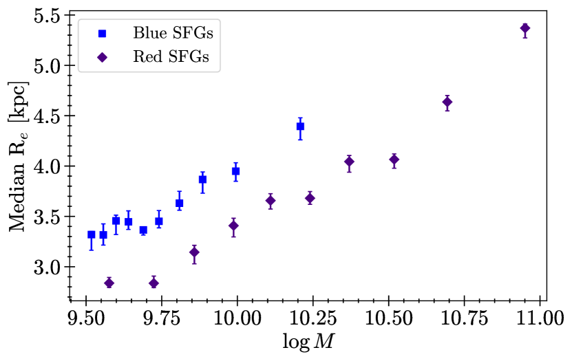
Figure 18: The median rest-frame $5000$ Å sizes of red SFGs ($U-V>1$) and blue SFGs ($U-V\leq 1$) in ten equally populated mass bins. The red SFGs are shown as indigo diamonds and blue SFGs as blue squares. All errors are bootstrapped. Blue SFGs tend to be less massive than red SFGs and thus mass bins are concentrated at lower masses for blue SFGs. At a given mass, blue SFGs are $20\%$ larger than red SFGs.

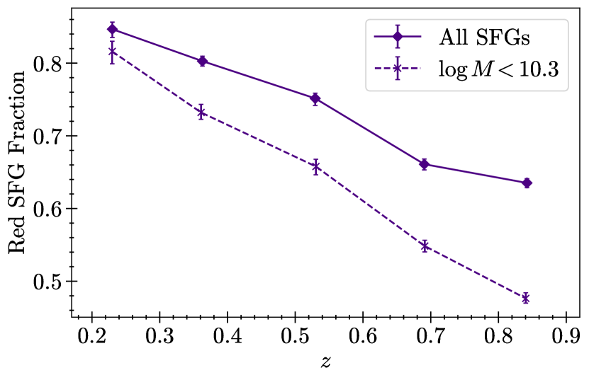
Figure 19: The redshift evolution of the SFG red fraction: fraction of red SFGs in the complete SFG population along with bootstrapped error bars (diamonds with solid line). Conversely, the fraction of blue SFGs decrease with cosmic time. We find that the fraction of red SFGs increases with cosmic time. Since the majority of blue SFGs have mass $\log M<10.3$ (see Figure 18), we also show the red SFG fraction in this mass range (crosses with dashed line) to demonstrate that the trend remains the same. This fractional increase in the smaller and redder SFGs with cosmic time could explain the slowing pace of the characteristic size evolution of SFGs since $z\sim 1$.

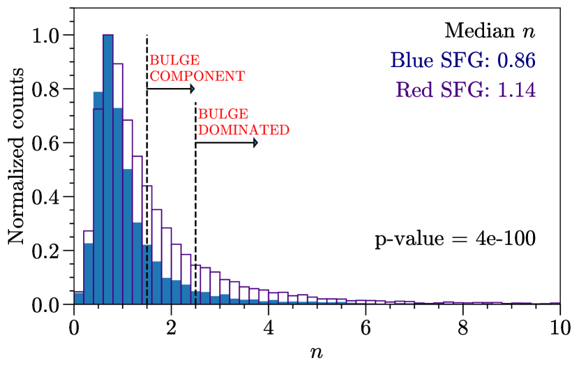
Figure 20: The distribution of Sérsic indices of blue SFGs (blue filled histograms) and red SFGs (purple unfilled histograms). Galaxies with $n>1.5$ are often considered to have a significant bulge component whilst galaxies with $n>2.5$ are considered to bulge dominated. Among bulge-dominated SFGs, $83\%$ are red. We also show the p-value from the K-S test in the figure legend.

We also find that the fraction of red galaxies in the SFG population is steadily increasing with cosmic time across the redshift range we explore (Figure 19). At $0.75<z<0.9$, red SFGs constitute $\sim 64\%$ of the SFG sample (purple diamonds with solid curve). This percentage increases to $\sim 80\%$ in the lowest redshift bin. Conversely, the fraction of blue SFGs decreases with redshift because the sum of fractions of red and blue SFGs equals to $1$ in each redshift bin.

Since blue SFGs have low masses, we investigate how the fraction of red SFGs change with redshift for $\log M<10.3$ (crosses with dashed curve in Figure 19). We find a similar trend: the fraction of red SFGs increases with decreasing redshift. Low-mass red SFGs constitute $\sim 48\%$ of the low-mass SFG sample in the highest redshift bin but this percentage increases to $\sim 82\%$ in the lowest redshift bin. This increase in the fraction of smaller red galaxies in the SF population could explain the observed slower pace of sizes growth for SFGs at $z<1$ with respect to higher redshifts.

Based on the observational studies, galaxies with Sérsic index $n\gtrsim 1.5$ are generally considered to have a significant bulge component and those with $n\gtrsim 2.5$ are considered bulge-dominated or spheroidal galaxies (e.g., Dutton, 2009; Sachdeva, 2013). Figure 20 shows that in our sample red SFGs dominate both the $n>1.5$ (galaxies with significant bulge component) and $n>2.5$ (bulge-dominated galaxies) subsamples with 81% and 83%, respectively. The average Sérsic indices of red SFGs are higher than their blue counterparts. The median $n$ of red SFGs ($n=1.14$) is $33\%$ higher than blue SFGs ($n=0.86$). We perform a Kolmogorov–Smirnov test (K-S test, Kolmogorov-Smirnov et al., 1933; Smirnov, 1948) to check whether the two distributions differ statistically from each other. An extremely small p-value implies that the two samples do not originate from the same parent (sub)population.

Even when we remove massive red SFGs and restrict the analysis of Sérsic indices to $\log M<10.3$, we find similar trends as in Figure 20. Among low-mass SFGs with significant bulge component, $\sim 69\%$ are red SFGs; among bulge dominated SFGs, this percentage is $\sim 72\%$.

To summarize, we see that blue SFGs are more extended but lower in mass than red SFGs. The fraction of red SFGs in the parent SFG population is increasing steadily with cosmic time. Red SFGs tend to be more concentrated and host significant bulge component in them compared to their bluer SFG counterparts. Together with the difference we see between sizes of SFGs at shorter and longer rest-frame wavelengths (Figures 12, 15, 16, and 17) and the scenarios that can explain it (Section 5.1.1), this analysis suggests that the emergence of bulges is driving the observed average size evolution of SFGs.

Several physical processes may be responsible for the emergence and growth of bulges in galaxies. Bulge growth can happen internally (secular evolution) or it can be induced externally.

In secular evolution, bulge formation and growth is often a result of perturbations in the galaxy disks due to internal substructures such as spiral arms and bars (Kormendy & Kennicutt, 2004; Athanassoula, 2005; Kormendy, 2008; Gadotti, 2009; Sellwood, 2014). This secular growth of bulges (also called pseudo-bulges) is global to all disk galaxies. The pseudo-bulges are characterised by disk like profiles ($n\sim 1$) and thus do not increase galaxy Sérsic index.

In contrast, bulge formation and growth induced externally (e.g., through mergers) by displacing the stars and gas in the disks towards galaxy centres, can contribute to the increase in galaxy Sérsic index (Naab et al., 2006; Gadotti, 2009; Hopkins et al., 2010; Oser et al., 2010; Tacchella et al., 2019). Bulges formed in this manner (classical bulges) have light profiles and properties similar to elliptical galaxies. These bulges have higher fraction of old red stars than in the disks and appear redder in colour (e.g., Breda et al., 2020). They generally have centrally concentrated surface brightness distributions, which are reflected in their higher $n$.

Several processes can cause a compaction towards galaxy centre resulting in central bulge formation and growth. Those mechanisms include galaxy wet mergers (Zolotov et al., 2015; Inoue et al., 2016) and collisions of counter-rotating gas streams that feed the galaxy (Danovich et al., 2015). In both cases, dissipative gaseous accretion promotes bursts of star formation and growth of stellar mass towards galaxy centre (e.g., Dekel et al., 2009; Lapiner et al., 2023). The absence of further gas inflow results in gas depletion and eventual quenching of the core regions (e.g., Ceverino et al., 2010; Zolotov et al., 2015; Tacchella et al., 2016). Thus, the bulges in SFGs tend to have high central mass concentrations and appear redder in colour as they age. We note, however, that wet compaction events are more common at earlier cosmic times than within the redshift interval we probe here.

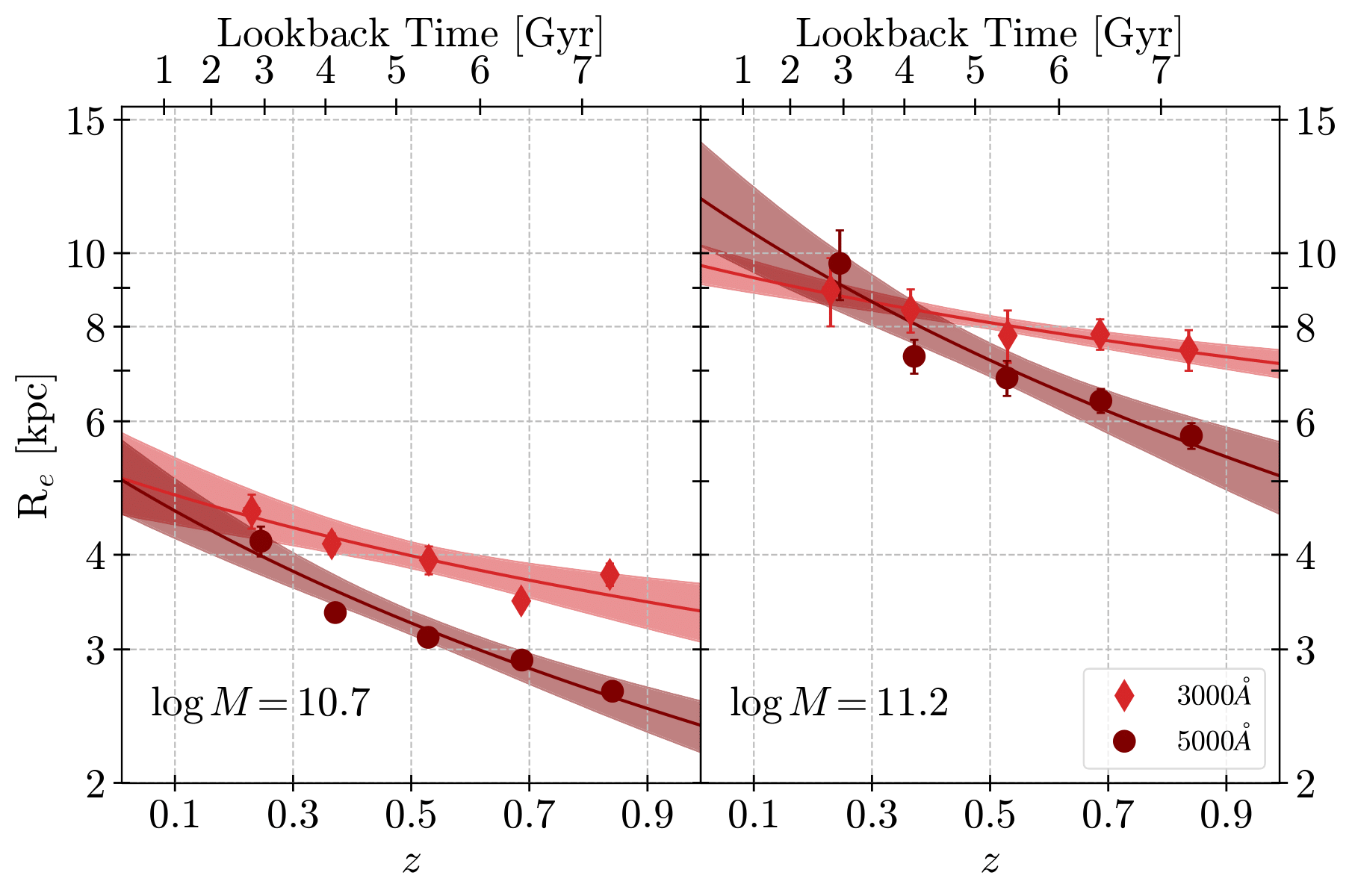
Figure 21: Evolution of median sizes of QGs. Panels show the size evolution of SFGs at two different characteristic masses. The QG sizes at rest-frame $3000$ Å is shown in red and at rest-frame $5000$ Å in maroon. The sizes at shorter wavelength is larger than those at longer wavelengths. The size evolution is fit using a power-law: $A(1+z)^{\beta}$ and the best fitting parameters are given in Table 4.3. The solid curves show the best-fit evolutionary curves with shaded regions showing their $1\sigma$ confidence intervals.

Studies based on cosmological hydrodynamic simulations (e.g., IllustrisTNG) predict that the emergence of centrally concentrated spheroidal components is a common phenomena in SFGs (e.g., Tacchella et al., 2019). Observational studies show that the overall Sérsic index and bulge-to-total ratios increase with cosmic time for SFGs which agrees with the predictions of simulations that the bulges are growing in SFGs (e.g., Lang et al., 2014). In light of these results, the emergence of classical bulges must be responsible for the high $n$ tail of the Sérsic index distribution for SFGs in our sample.

5.1.4 Limitations

Effects of age and metallicity on galaxy light profiles cannot be disentangled without spatially-resolved spectroscopic data. Observed larger galaxy sizes in shorter wavelength can result from either young or low-metallicity stars in their outskirts as both stellar population properties contribute to galaxy colours (e.g., Gustafsson, 1989; Streich et al., 2014). If light profiles of our $\log M>9.5$ SFGs in bluer rest-frame wavelength are at least in part affected by the presence of low-metallicity stars, measured larger sizes in $3000$ Å can point towards accretion (in addition to star-formation) in the outskirts of these galaxies. Low mass galaxies generally have lower metallicities than massive ones (e.g., Tremonti et al., 2004; Foster et al., 2012; Zahid et al., 2014; Ma et al., 2016). Thus the accretion of low-mass satellites can lower the average metallicity and increase the surface brightness of galaxy outskirts in bluer light.

The presence of dust can also cause observed differences between rest-frame $3000$ Å  and $5000$ Å. The rest-frame $3000$ Å is more impacted by dust absorption than $5000$ Å. Some studies show that the dust attenuation is stronger in bulges than in disks (e.g., Driver et al., 2007). This radial dependence of dust reddening could impact the fitting of Sérsic profile at $3000$ Å. As the contribution of unobscured blue light from the outskirts dominates the overall light profile of a galaxy, its $R_{e}$ is overestimated and $n$ is underestimated. However, we find that the red SFGs tend to be smaller and have higher Sérsic indices than blue SFGs in the rest-frame $5000$ Å where galaxy light is less affected by dust compared to the rest-frame $3000$ Å (Figures 18 and 20). Hence, we conclude that the observed differences between red and blue SFGs in our study are not driven by dust reddening alone.

With this study, we do not perform detailed analysis of galaxy components (bulges v/s disks). This is a necessary next step in testing the bulge growth scenario for the size evolution of SFGs. In the follow-up study we plan to perform bulge-disk decomposition and estimate bulge-to-total (B/T) ratios for all CLAUDS+HSC galaxies using a multi-component model fitting approach.

5.2 Size Evolution of Quiescent Galaxies

5.2.1 Overview of the Observed Trends

As in Section 5.1, we use characteristic sizes estimated from the SMR to trace the evolution in size for QG population in two rest-frame waveleghts (Figure 21). We limit the analysis to two different characteristic masses ($\log M=10.7,11.2$) that are above the pivot point of the SMR (Section 4.1) for quiescent population.

As expected, the results we show in Figure 21 are in line with our findings in Section 4.3. Similar to SFGs, we find that the sizes of QGs are larger in rest-frame $3000$ Å  than in $5000$ Å (red and maroon curves in Figure 21). At $z\sim 0.5$, QGs with mass $\log M=10.7$ are $\sim 23\%$ larger in size in shorter wavelength than in longer wavelength. This offset in size decreases with increase in stellar mass. At the same redshift, QGs with mass $\log M\sim 11.2$ are $\sim 12\%$ more extended in the rest-frame UV light than in visible light.

With respect to SFGs in our sample, QGs exhibit much stronger size evolution in rest-frame $5000$ Å than in $3000$ Å. For example, in the rest-frame $3000$ Å, QGs with mass $\log M\sim 10.7$ grow in size by $\sim 38\%$ in the rest-frame UV and by $\sim 82\%$ in the rest-frame visible light over the span of 6 Gyrs that we probe. For very massive QGs ($\log M\sim 11.2$), this growth is by $\sim 27\%$ and $\sim 97\%$, respectively, for sizes measured in rest-frame UV and visible light.

Furthermore, the average size of a QG is significantly smaller than an SFG at a given mass and redshift (Figure 15). Comparison of the last two panels of Figure 16 with Figure 21 shows that at $z=0.5$ and rest-frame wavelength $5000$ Å, $\log M=10.7$ SFG is $\sim 70\%$ larger than QG of the same stellar mass. However, SFGs and QGs with $\log M=11.2$ have similar sizes. The trends in the bluer wavelength are also similar to those in the redder wavelength. This is interpreted to be due to the fading of disk when a galaxy fully quenches (e.g., Christlein & Zabludoff, 2004; Carollo et al., 2016; Matharu et al., 2020; Estrada-Carpenter et al., 2023). Since the disks are more extended than their more centrally concentrated bulges/spheroids, the overall size of a galaxy shrinks when the disk completely fades.

Alternatively, the smaller sizes of QGs relative to SFGs of comparable stellar mass could be due to the preferential growth of central regions over the outer ones during and after quenching. We can investigate the effects of both disk fading and growth of bulges through bulge$+$disk decomposition in two rest-frame wavelengths. When the star formation in galaxy disk is quenched, the disk become fainter, especially at UV wavelengths (although it does not disappear completely). The surface brightness of the disk diminishes significantly in the rest-frame UV regime and less so at longer (rest-frame optical) wavelengths. However, this fading should not affect the central regions (galaxy bulges). We will explore this effect in our future work through bulge$+$disk decomposition.

Finally, the QGs tend to grow in size at a more rapid pace compared to SFGs even though they do not actively form stars. This observation is in line with the literature (e.g., Conselice, 2014; van der Wel et al., 2014; Straatman et al., 2015; Damjanov et al., 2019; Kawinwanichakij et al., 2021). This strong size evolution could be driven by several physical processes affecting individual QGs, such as major mergers (Conselice et al., 2003, 2022; Bluck et al., 2012; Kaviraj et al., 2014; Man et al., 2016; Mantha et al., 2018; Huško et al., 2022, 2023), minor mergers and accretion (Khochfar & Silk, 2006; Naab et al., 2009; Bluck et al., 2012; Newman et al., 2012; Fagioli et al., 2016; Sawicki et al., 2020; Conselice et al., 2022; Huško et al., 2023; Suess et al., 2023), and adiabatic expansion (Boily & Kroupa, 2003; Goodwin & Bastian, 2006; Baumgardt & Kroupa, 2007; Fan et al., 2008, 2010; Damjanov et al., 2009; Ragone-Figueroa & Granato, 2011; Lapi et al., 2018). In addition, progenitor bias due to newcomers affects the average QG size evolution (Franx et al., 2008; Carollo et al., 2013; Fagioli et al., 2016; Damjanov et al., 2019, 2023).

Galaxy mergers can contribute significantly to the size evolution of QGs. Although major dry mergers can yield an increase in size of QGs proportional to the increase in mass (eg., Boylan-Kolchin et al., 2006; Naab et al., 2007), the average number of major mergers per galaxy since $z\sim 1$ is low (e.g., Bundy et al., 2009; López-Sanjuan et al., 2010; Kaviraj et al., 2014; Thibert, 2018). However, both observational studies (e.g., Bezanson et al., 2009; van Dokkum et al., 2010; Trujillo et al., 2011; Fagioli et al., 2016; Zahid et al., 2019) and theoretical/simulation based studies (e.g., Khochfar & Silk, 2006; Naab et al., 2009; Oser et al., 2010, 2012; Hilz et al., 2012) show that minor mergers and accretion can support size growth in QGs. Theoretical studies (e.g., Naab et al., 2009) and observational studies that incorporate these theoretical predictions (e.g., Bezanson et al., 2009; Zahid et al., 2019) indicate that a series of minor mergers, with the fractional growth in $R_{e}\propto M_{*}^{2}$ (where $M_{*}$ is the fractional growth in stellar mass) can explain QG size growth since $z\sim 2-3$.

The fact that the QGs have larger sizes in shorter wavelength (red curves in Figure 21) than the longer one (maroon curves in Figure 21) could indicate growth through minor mergers and accretion (e.g., Bezanson et al., 2009; Naab et al., 2009; Suess et al., 2020, 2023). As these are passive galaxies, they are not actively forming stars, but the bulk of the young and/or low-metallicity stars traced by shorter wavelength could be added ex-situ or formed from ex-situ added gas through accretion and minor mergers. These materials are added to the outskirts puffing up galaxy light profile.

On the other hand, the longer wavelength profiles are dominated by the in-situ old stars which are concentrated towards galaxy centre. As time progresses, the ex-situ stars can also migrate inward and add to the galaxy profile in the longer wavelength as they age (e.g., Boecker et al., 2023). Since the longer wavelength probes newly added old ex-situ stars along with the already existing in-situ aged stellar population in galaxies, we see the stronger evolution in rest-frame $5000$ Å.

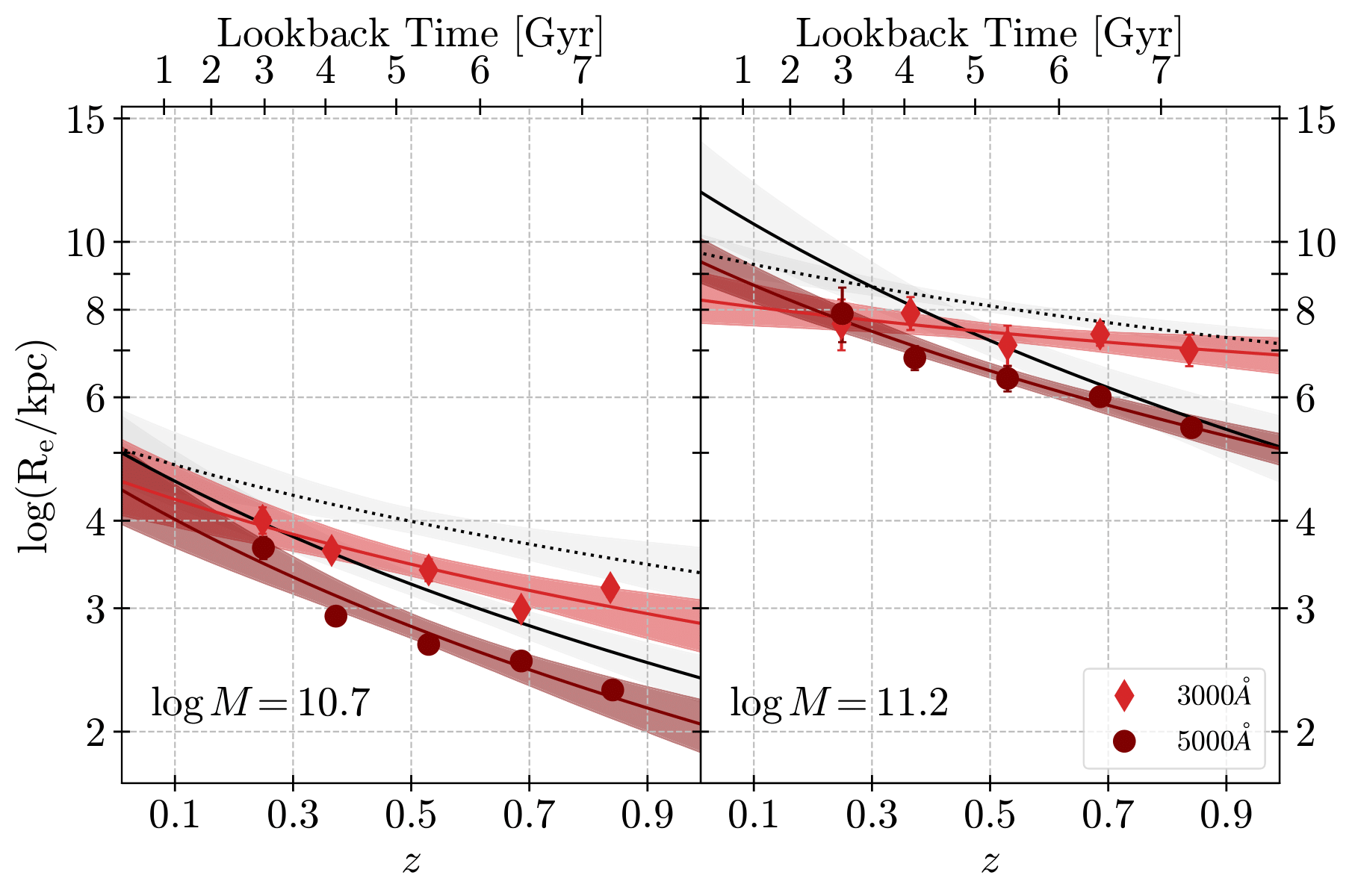
Figure 22: Size Evolution of QGs in two rest-frame wavelengths when progenitor bias is removed. The size evolution curves of the entire QG population are shown in gray (dotted and solid curves for rest-frame UV and visible light respectively). The best-fit parameters are given in Table 5.2.2. Other details are same as for Figure 21.

5.2.2 Removing the Effect of Progenitor Bias

Newly quenched galaxies (newcomers) can affect the distribution of QG sizes at a given mass because they are, on average, more extended than the rest of the QG population (progenitor bias; Saglia et al., 2010; Damjanov et al., 2023). Progenitor bias should not contribute significantly to the size evolution of QGs. For example, Damjanov et al. (2023) find that the newcomers contributed only $11\%$ to the growth of QGs at $z<0.6$. Nonetheless, it is important to remove the impact of progenitor bias from the QG population to understand how aging QGs may evolve with time. Here we account for the effect of progenitor bias by removing the most extended galaxies and re-fitting the “corrected" QG SMR in five redshift bins that cover the $0.1<z<0.9$ interval.

We assume that in total $\sim 10\%$ of the QG population above the SMR pivot point in each redshift bin are newcomers (Moutard et al., 2016). However, the probability for an SFG to quench increases with stellar mass and is given by

$$\begin{split}p_{Q}&\varpropto\left(1-e^{-\frac{M}{M^{*}}}\right),\\ &=c\left(1-e^{-\frac{M}{M^{*}}}\right),\end{split}$$ (13)

where $M$ is the stellar mass of the SFG in solar masses, $c$ is the normalization constant and $M^{*}$ is the characteristic mass from stellar mass (Schechter) function for SFGs in M_⊙ (Peng et al., 2010b). $M^{*}$ varies with redshift and we adopt the values from Muzzin et al. (2013). In addition, the number densities of SFGs and QGs also vary with stellar mass and redshift (e.g., Muzzin et al., 2013).

To incorporate this information into a toy model of QG size growth, we first divide massive QGs ($M>M_{p}$) in each redshift bin into $10$ equal frequency bins of stellar mass. Then we determine the fraction of galaxies to be removed from each mass bin as

$$f_{pb}=p_{Q}\frac{n_{Q}(M)}{n_{T}(M)},$$ (14)

where $n_{Q}(M)$ and $n_{T}(M)$ are the number densities of QGs and all galaxies respectively. We adopt the number densities from Muzzin et al. (2013). We use the normalization constant $c$ in the equation for $p_{Q}$ (Equation 13) to keep the percentage of the newly quenched galaxies to be $\sim 10\%$ . We adopt $c=3/5$ which removes $\sim 8-13\%$ of the most extended galaxies in each redshift bin above the SMR pivot point (see also Appendix C). Across the stellar mass bins, this percentage varies from $\sim 0\%$ to $\sim 20\%$ of the QG population in that bin. We then perform the SMR fitting and examine the evolution of characteristic sizes of remaining (aging) QGs at two different stellar masses in $3000$ Å and $5000$ Å (Figure 22; the best-fit parameters of the size evolution are given in Table 5.2.2).

cccc[hvlines]

1-4QGs

Restframe $\lambda$ $\log M_{(z=0.9)}$ $R_{e}^{0}$ $\beta$

2-1$3000$ Å $10.7$ $4.58\pm 0.60$ $-0.69\pm 0.28$

$11.2$ $8.28\pm 0.70$ $-0.27\pm 0.19$

2-1$5000$ Å $10.7$ $4.48\pm 0.59$ $-1.13\pm 0.29$

$11.2$ $9.45\pm 0.70$ $-0.91\pm 0.17$

Table 5: The parameters of the best-fit power-law (Equation 10) to the redshift evolution of characteristic QG sizes after the removal of the the progenitor bias (Section5.2).

When we remove the supposed newcomers from the QG sample, the average characteristic sizes of QGs become smaller, as expected. The decrease in the average size of QGs with stellar mass $\log M=10.7$ is similar across the redshift range at both wavelength regimes ($11-15\%$). However, at high stellar mass ($\log M=11.2$), this decrease ranges from $3\%$ ($5\%$) at $z=0.9$ to $18\%$ ($13\%$) at $z=0.1$ in rest-frame visible (UV) light.

We do not find any significant difference in the pace of size growth for QGs with mass $\log M=10.7$ when we account for progenitor bias in both wavelength regimes (compare coloured curves against black curves in the first panel of Figure 22). However, there are indications that the size evolution becomes weaker when we remove the progenitor bias for QGs with mass $\log M=11.2$ (second panel of Figure 22). Nonetheless, the difference is within uncertainties for both UV and visible light. Thus, the progenitor bias only causes a significant vertical offset in the redshift evolution of average QG sizes without strong signals of change in the exponent of the evolutionary trends for stellar masses higher than the pivot mass ($\log M\sim 10.5$, Section 4.1).

Progenitor bias can affect the size evolution of QGs in two ways. First, the sizes of SFGs are larger than QGs at the same stellar mass and the size of SFGs increase with time (e.g., Figures 11 and 15). Thus, the newcomers are larger than the those quenched earlier in time. This causes a vertical shift in the size evolution curve by increasing the average size of QGs at all redshifts. We see this effect in our sample (the black curves are higher than coloured curves in Figure 22).

Second, disks of galaxies fade when they quench (Christlein & Zabludoff, 2004; Carollo et al., 2016; Estrada-Carpenter et al., 2023). Bulge becomes more prominent in a galaxy light profile resulting in smaller effective sizes of galaxies. Since the disk fading affects light profiles in rest-frame $3000$ Å more than $5000$ Å and the quenched fraction increases with cosmic time, the progenitor bias effect should slow down the pace of size evolution in the shorter wavelength (red curves in Figure 22). We expect to see a strengthening of the size evolution for QGs in rest-frame UV light after we remove the progenitor bias. Instead, we find that the pace of the size evolution is unaffected indicating that the process of disk fading does not affect the average size evolution of massive QGs.

Thus, we conclude that the effects of progenitor bias on the massive QG population is mainly on the vertical offset of the evolutionary trend. The strength of the redshift evolution in size for massive QGs is determined by other physical processes such as minor mergers and accretion adding low-mass and/or low-metallicity stellar population (Section 5.1.4) to galaxy outskirts.

5.3 Evolution in Central Stellar Mass Surface Density

Central stellar mass surface density, the projected stellar mass surface density within central $1$ kpc radius, is another physical parameter that is widely used in the analysis of galaxy evolution (e.g., Cheung et al., 2012; Fang et al., 2013; Barro et al., 2013, 2014, 2017; Suess et al., 2021, 2020; Xu & Peng, 2021; Ji et al., 2022; Ji & Giavalisco, 2022, 2023; Estrada-Carpenter et al., 2023). Stellar mass surface density is derived using both $R_{e}$ and $n$ and thus it does not include uncertainties due to covariance between $R_{e}$ and $n$ making it a more robust parameter than these two parameters individually (Ji et al., 2020, 2022).

We calculate $\Sigma_{1}$ in units of $\hbox{M${}_{\odot}$}/\text{kpc}^{2}$ and fit the relation between $\Sigma_{1}$ and galaxy stellar mass in Appendix D. We first fit the $\Sigma_{1}$-stellar mass relation in log-log space for all SFGs and QGs (Figure 31) and also for SFGs split into blue and red subpopulations (Figure 32). One of the parameters of the fits we perform in Appendix D is the characteristic $\Sigma_{1}$ value for galaxies with stellar mass of $5\times 10^{10}$ M_⊙. Figure 23 shows the redshift evolution of this characteristic value for SFGs (dark blue stars) and QGs (maroon filled circles).

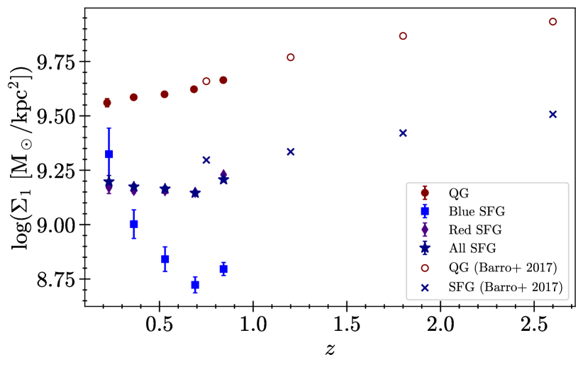
Figure 23: The evolution of characteristic $\Sigma_{1}$ for galaxies with mass $5\times 10^{10}$ M_⊙. We show these values for all SFGs (dark blue stars) and QGs (maroon dots) along with their uncertainties. We also show the evolution in $\Sigma_{1}$ in two subpopulations of SFGs - blue (blue diamonds) and red (purple squares). We compare our results with the estimated characteristic $\Sigma_{1}$ values at higher redshift for SFGs (blue crosses) and QGs (maroon open circles) from Barro et al. (2017).

The QGs have $\sim 2$ ($3$) times higher $\Sigma_{1}$ than SFGs at $0.1<z<0.3$ ($0.75<z<0.9$). As the majority of the SFGs are red (Figure 19), the average $\Sigma_{1}$ of red SFGs (purple diamonds) are almost identical to those of all SFGs. However, blue SFGs (blue squares) have significantly lower $\Sigma_{1}$ values than red SFGs, except at $0.1<z<0.3$ where the sample size is small. Red SFGs have $\sim 1.5$ ($2.7$) times higher central stellar mass density than blue SFGs at $0.3<z<0.45$ ($0.75<z<0.9$). This difference is in line with SFGs growing their central regions and increasing $\Sigma_{1}$ during their evolution towards the red sequence (as also reported by Guo et al., 2021; Quilley & de Lapparent, 2022).

We compare our results with the evolution in $\Sigma_{1}$ for SFG and QG at $0.5<z<3$ (Barro et al., 2017, maroon open circles (QGs) and blue crosses (SFGs) in Figure 23). High-redshift $\Sigma_{1}$ are estimated based on spatially resolved SED fits derived from surface brightness profiles in nine HST bands. We do not have spatially resolved SED fits for $z<1$ galaxies. By incorporating spatially resolved SEDs, Barro et al. (2017) are potentially able to incorporate the effects of colour gradients in the $\Sigma_{1}$ calculation. However, these gradients in both SFGs and QGs do not evolve at $z<1$ significantly (Suess et al., 2019). Hence, the fact that we consider only global rather than spatially resolved colour gradients does not affect the difference in the evolutionary trends for $\Sigma_{1}$ between two studies.

Figure 23 shows decreasing trend in $\Sigma_{1}$ of SFGs at $z>1$ with cosmic time. At $z<1$, we find that the SFGs with mass $5\times 10^{10}$M_⊙ have, on average, a constant $\Sigma_{1}$ value. We interpret this lack of evolution in $\Sigma_{1}$ for SFGs in our sample as another aspect of prominent bulge growth in them. The growth of centrally concentrated bulges increases the $\Sigma_{1}$ values at lower redshift, resulting in flattening of the observed evolutionary trend.

The characteristic $\Sigma_{1}$ values for QGs also decrease with time since $z\sim 3$. Potential mechanisms driving this decrease in $\Sigma_{1}$ include minor mergers (resulting in much larger size than stellar mass increase; e.g., Bezanson et al., 2009; Hopkins et al., 2009; Naab & Ostriker, 2009; van Dokkum et al., 2010; Fagioli et al., 2016; Zahid et al., 2019), adiabatic expansion due to mass loss and the rearrangement of stellar orbits in shallower gravitational potential (e.g., Damjanov et al., 2009, 2011; van Dokkum et al., 2010, 2014; Lapi et al., 2018), and the influx of larger newcomers (Section 5.2.2; Carollo et al., 2013; Damjanov et al., 2019, 2023; Ji & Giavalisco, 2022).

However, QGs at $z<1$ show that the pace of redshift evolution in $\Sigma_{1}$ slows down at $z<0.9$. For example, $\Sigma_{1}$ of QGs decreases by $\sim 10\%$ from $z\sim 0.7$ to $z\sim 0.2$ (or over 4 Gyrs of cosmic time), while the decline is somewhat more dramatic at higher $z$ ($20\%$ between the redshift bins $1.5<z<2$ and $1<z<1.5$, corresponding to $\sim 2$ Gyrs of cosmic time). This weakening of $\Sigma_{1}$ evolution reflects the lack of evolution in $\Sigma_{1}$ for SFGs (especially red SFGs shown in purple diamonds) of the same mass. This similarity in trends between SFGs and QGs is driven partly by the quenching processes that transfer a fraction of SFGs in one redshift bin to the the QG population in the next lower redshift bin.

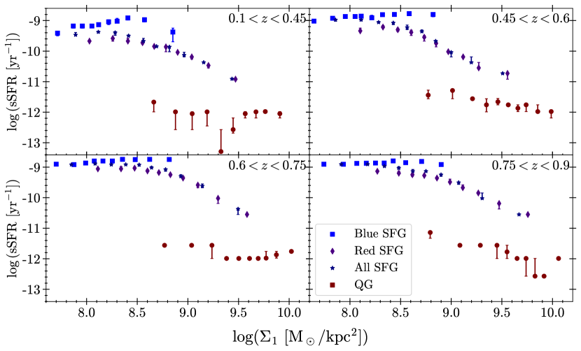
Figure 24: The relation between specific star formation rate (sSFR) and $\Sigma_{1}$ in four redshift bins for SFGs (red, blue and all) and QGs. We divide each galaxy groups into $10$ equally populated bins of $\Sigma_{1}$ and estimate median sSFR. The errorbars correspond to the bootstrapped errors for the medians.

Earlier studies show that galaxy star formation activity is correlated with their central stellar mass surface density (e.g., Barro et al., 2017; Whitaker et al., 2017; Suess et al., 2021). These studies demonstrate that galaxies follow an "L-shaped track" in the specific star formation rate (sSFR) vs $\Sigma_{1}$ parameter space. We explore this relation in Figure 24, where we show median sSFR values for both SFGs (dark blue stars) and QGs (maroon filled circles) in ten equally populated $\Sigma_{1}$ bins. The sSFR values for SFGs are roughly stable at $\log\Sigma_{1}\lesssim 9$. After that point, the sSFR starts to decrease with the increase in $\Sigma_{1}$. As the SFGs build up their central regions, their star-formation activity declines. However, we note that the observed correlation between $\Sigma_{1}$ and the sSFR may not necessarily imply a causal relation between the two parameters since a third, hidden parameter may be involved (as also noted by, e.g., Lilly & Carollo, 2016; Chen et al., 2020; Ji & Giavalisco, 2022, 2023).

When we divide the SFG population into red and blue SFGs (purple diamonds and blue squares, respectively, in Figure 24), red SFGs show somewhat lower sSFR at any given $\Sigma_{1}$. Furthermore, there is a maximum $\Sigma_{1}$ above which only red SFGs exist.

The sSFR values for blue SFGs do not change with $\Sigma_{1}$, indicating that these young SFGs are actively forming stars at all galactocentric radii. The sSFR for red SFGs declines with $\Sigma_{1}$ above the threshold value where blue SFGs are absent. This trend suggests that by probing the red SFG subpopulation, we trace how these galaxies build up their central bulges and undergo inside-out quenching.

The threshold $\Sigma_{1}$ value above which all SFGs are red is $\log\Sigma_{1}\sim 9$. This threshold value does not evolve with redshift. In line with the values reported by Whitaker et al. (2017), our result suggests that as SFGs build up sufficient central stellar mass density, quenching process becomes prominent above this universal minimum value.

In addition, we find that there is a threshold $\Sigma_{1}$ ($\log\Sigma_{1}\sim 9.7$) beyond which a galaxy cannot sustain star formation. This finding broadly agrees with previous results of Whitaker et al. (2017), Suess et al. (2021) and Estrada-Carpenter et al. (2023).

Thus, we observe the minimum value for $\Sigma_{1}$ that corresponds to the point when quenching becomes prominent globally (throughout the galaxy) and the maximum value above which all galaxies are quiescent. Between these two threshold values of $\Sigma_{1}$, red bulges continue to grow in SFGs as indicated by the negative correlation between $\Sigma_{1}$ and sSFR (Figure 24).

The range of $\Sigma_{1}$ values that red SFGs can have once they drop below sSFR for the blue subpopulation suggests that the process we trace is the slow process of bulge growth that drives this decline in sSFR. A number of studies support the emergence/significant growth of centrally concentrated bulges in galaxies before and while they transition through the green valley and quench (Barro et al., 2017; Wu et al., 2020; Guo et al., 2021; Quilley & de Lapparent, 2022; Ji & Giavalisco, 2023). Therefore, we conclude that the bulge growth is the major driving force behind the evolution of SFGs towards the red sequence at $z<0.9$.

6 Conclusions

We measure morphological parameters for 21,200 massive ($\log M>9.5$) star-forming and quiescent galaxies (SFGs and QGs) in the redshift range $0.1<z<0.9$ and in two rest-frame wavelengths, $3000$ Å and $5000$ Å. We use the multi-band images from the central region of the COSMOS field in the CLAUDS+HSC Survey and ancillary data from COSMOS2020 catalogue for the estimates of galaxy redshifts and stellar masses. We measure galaxy sizes by fitting a single-component Sérsic profile to their light profiles using Galfit software.

We fit the size-mass relation (SMR) for SFGs and QGs separately in five redshift bins in the two rest-frame wavelengths (Equations 7 and 8. We then analyse the redshift evolution of galaxy sizes by fitting a power-law (Equation 10).

The main conclusions of our study are:

1. Both SFGs and QGs on average appear more extended in blue light (rest-frame $3000$ Å) than in red light (rest-frame $5000$ Å) at all redshifts and masses (Figures 12, 15, 16 and 21). We find that the pace of evolution at fixed stellar mass is stronger in the rest-frame visible light than in the rest-frame UV light and this difference is more prominent for QGs (Figure 21). In addition, the strength of the evolution in both wavelengths in general increases with the stellar mass of galaxies (Figures 15 and 16).

2. When we incorporate mass growth for SFGs assuming the evolving star formation main sequence, the pace of the SFG size evolution (i.e., the exponent of the best-fitting power-law) becomes independent of both galaxy stellar mass and the rest-frame wavelength (Figure 17).

3. The strength of the size evolution at constant stellar mass for SFGs is weaker than the strength reported in studies that cover wider redshift ranges. We explore this slowing down of the size evolution since $z\sim 1$ by dividing the SFG population into two groups: blue SFGs ($U-V\leq 1$) and red SFGs ($U-V>1$). We find that red SFGs are smaller and more massive than blue SFGs and that their fraction increases by $25\%$ during the $6$ billion years of cosmic time that we explore. In addition, red SFGs constitute the majority ($83\%$) of the bulge-dominated SFGs ($n>2.5$). We conclude that the emergence of bulges is a primary driver of size evolution for SFGs.

4. We use a a toy model to remove the effect of newcomers (progenitor bias) from the observed trend in size evolution for QGs. The removal of the largest QGs changes the characteristic size of QGs at $z=0$ ($R_{e}^{0}$ in Equation 10). This change in $R_{e}^{0}$ is systematically negative for all masses and in both rest-frame wavelengths. Our analysis shows that newcomers increase the average size of QGs by up to $\sim 20\%$ since $z\sim 1$. In contrast, the pace of QG size evolution is not affected systematically by this effect. We conclude that the strength of the evolution is not determined by disk fading during the process of quenching but rather by physical processes affecting individual galaxies after they become quiescent (e.g., mergers and accretion).

5. We find that the redshift evolution of $\Sigma_{1}$ stops (slows down) for SFGs (QGs) at $z<1$. This change in the evolutionary pace compared to higher $z$ is consistent with the growth of bulges in SFGs and the influx of newcomers to the QG population. We also find that all SFGs with $\log\Sigma_{1}\gtrsim 9$ are red ($U-V>1$) and that all galaxies with $\log\Sigma_{1}\gtrsim 9.7$ are quiescent. Finally, the sSFR of red SFGs within these two threshold values of $\Sigma_{1}$ declines with $\Sigma_{1}$, suggesting that the growth of bulges drives the evolution of SFGs towards the QG population.

To explore further the role of bulges in the average size growth of the SFG population and the impact of various physical processes on the QG size evolution, we will perform bulge$+$disk decomposition. We plan to implement this procedure in the future by fitting a double-component Sérsic profile to galaxy light profiles. Furthermore, here we do not investigate the impact of environment on the galaxy size evolution due to the small volume we probe. To take into account environmental effects, we will expand our analysis based both on a single- and double-component Sérsic profile to the entire $18.6$ deg² of the CLAUDS+HSC survey. Our pilot study demonstrates the power of deep ground-based photometric surveys and galaxy light profiles fitting in multiple rest-frame wavelengths to probe in detail the strength of galaxy structural evolution at $z<1$ and constrain its driving mechanisms.

Acknowledgements

We thank the anonymous referee for their thoughtful suggestions that helped us improve the clarity and completeness of the manuscript. We gratefully acknowledge the contributions of Anneya Golob, Bobby Sorba, Harrison Souchereau and Ikuru Iwata. We thank the extra-galactic research group at Saint Mary’s University, Canada, especially Vicente Estrada-Carpenter, Lingjian Chen and Devin Williams for their valuable inputs and support. We also thank Lalitwadee Kawinwanichakij, Dan Taranu, Connor Bottrell, Arjen van der Wel, Chien Peng, Lamiya Mowla and Jasleen Matharu for helpful discussions. The research of A.G., I.D. and M.S. is supported by the National Sciences and Engineering Council (NSERC) of Canada.

These data were obtained and processed as part of the CFHT Large Area U-band Deep Survey (CLAUDS), which is a collaboration between astronomers from Canada, France, and China described in Sawicki et al. (2019). CLAUDS is based on observations obtained with MegaPrime/ MegaCam, a joint project of CFHT and CEA/DAPNIA, at the CFHT which is operated by the National Research Council (NRC) of Canada, the Institut National des Science de l’Univers of the Centre National de la Recherche Scientifique (CNRS) of France, and the University of Hawaii. CLAUDS uses data obtained in part through the Telescope Access Program (TAP), which has been funded by the National Astronomical Observatories, Chinese Academy of Sciences, and the Special Fund for Astronomy from the Ministry of Finance of China. CLAUDS uses data products from TERAPIX and the Canadian Astronomy Data Centre (CADC) and was carried out using resources from Compute Canada and Canadian Advanced Network For Astrophysical Research (CANFAR).

The Hyper Suprime-Cam (HSC) collaboration includes the astronomical communities of Japan and Taiwan, and Princeton University, USA. The Hyper Suprime-Cam (HSC) collaboration includes the astronomical communities of Japan and Taiwan, and Princeton University. The HSC instrumentation and software were developed by the National Astronomical Observatory of Japan (NAOJ), the Kavli Institute for the Physics and Mathematics of the Universe (Kavli IPMU), the University of Tokyo, the High Energy Accelerator Research Organization (KEK), the Academia Sinica Institute for Astronomy and Astrophysics in Taiwan (ASIAA), and Princeton University.

This paper is based (in part) on data collected at the Subaru Telescope and retrieved from the HSC data archive system, which is operated by Subaru Telescope and Astronomy Data Center (ADC) at National Astronomical Observatory of Japan. Data analysis was in part carried out with the cooperation of Center for Computational Astrophysics (CfCA), National Astronomical Observatory of Japan.

Software: NumPy (van der Walt et al., 2011; Harris et al., 2020), SciPy (Virtanen et al., 2020), Astropy (Astropy Collaboration et al., 2013, 2018, 2022), Photutils (Bradley et al., 2022), PetroFit, Scikit-learn (Pedregosa et al., 2011), Matplotlib (Hunter, 2007), GalfitPyWrap, SExtractor (Bertin & Arnouts, 1996), PSFEx (Bertin, 2011), Galfit (Peng et al., 2002, 2010a), Dynesty (Speagle, 2020).

Data Availability

Hyper Suprime-Cam Subaru Strategic Program (HSC-SSP) Public Data are available at https://hsc.mtk.nao.ac.jp/ssp. CLAUDS u-band images of Deep and UltraDeep layers of the HSC-SSP and a catalogue that includes the parameters of the best-fit 2D Sérsic models we produced for this paper as well as matched COSMOS2020 photometry, stellar masses, and SFRs are available at https://www.clauds.net.

Appendix A Robustness of the Fitting Pipeline and Sérsic parameters

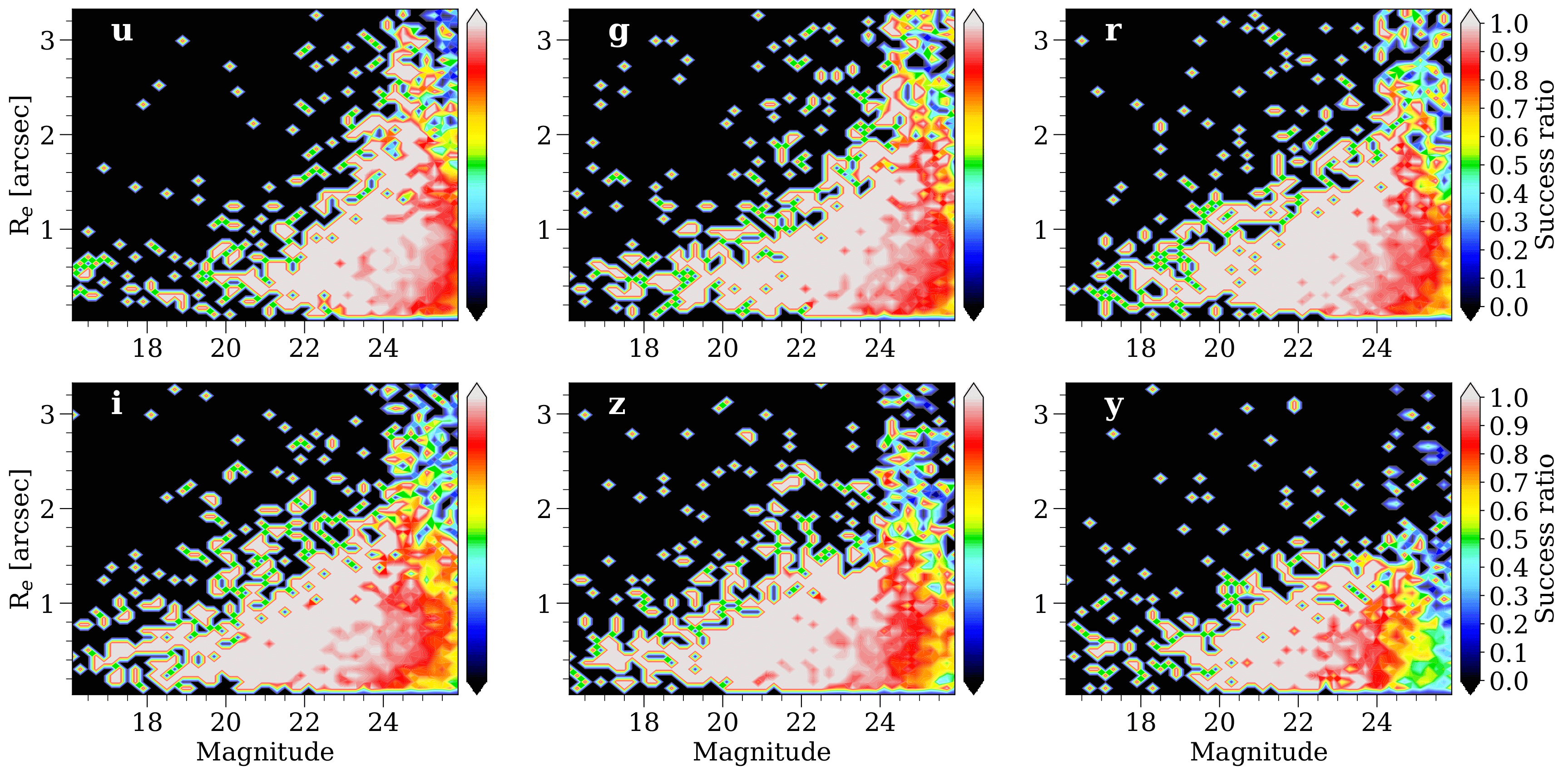
Figure 25: Heat maps showing the simulation success rate (Equation 4) as a function of input magnitude and input size. Galaxy sizes do not affect the success rate significantly in a given magnitude bin as indicated by the (almost) vertical colour stripes.

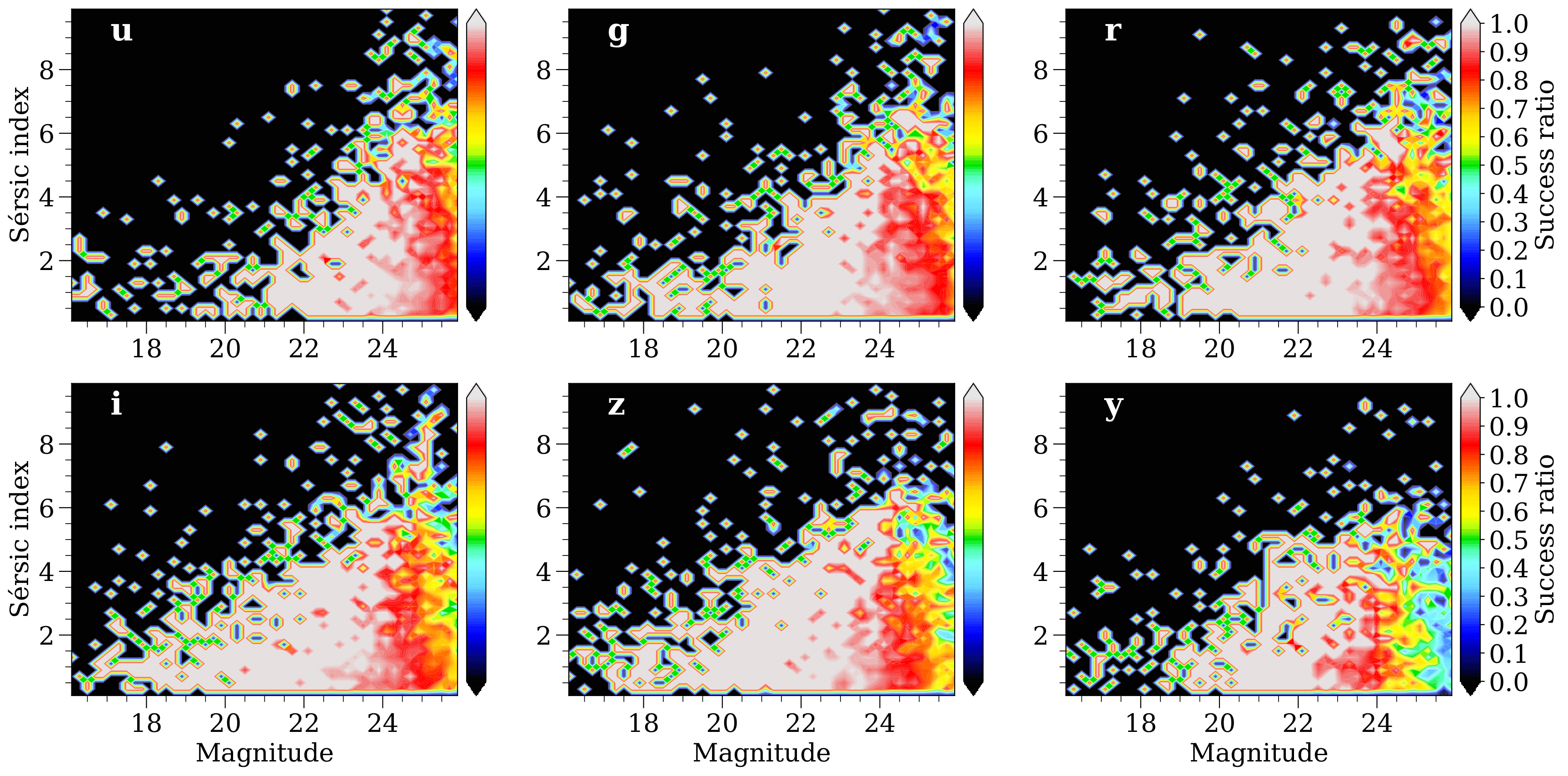
Figure 26: Heat maps showing the simulation success rate (Equation 4) as a function of input magnitude and input Sérsic index. Sérsic indices of galaxies do not affect the success rate significantly in a given magnitude bin as indicated by the vertical colour stripes.

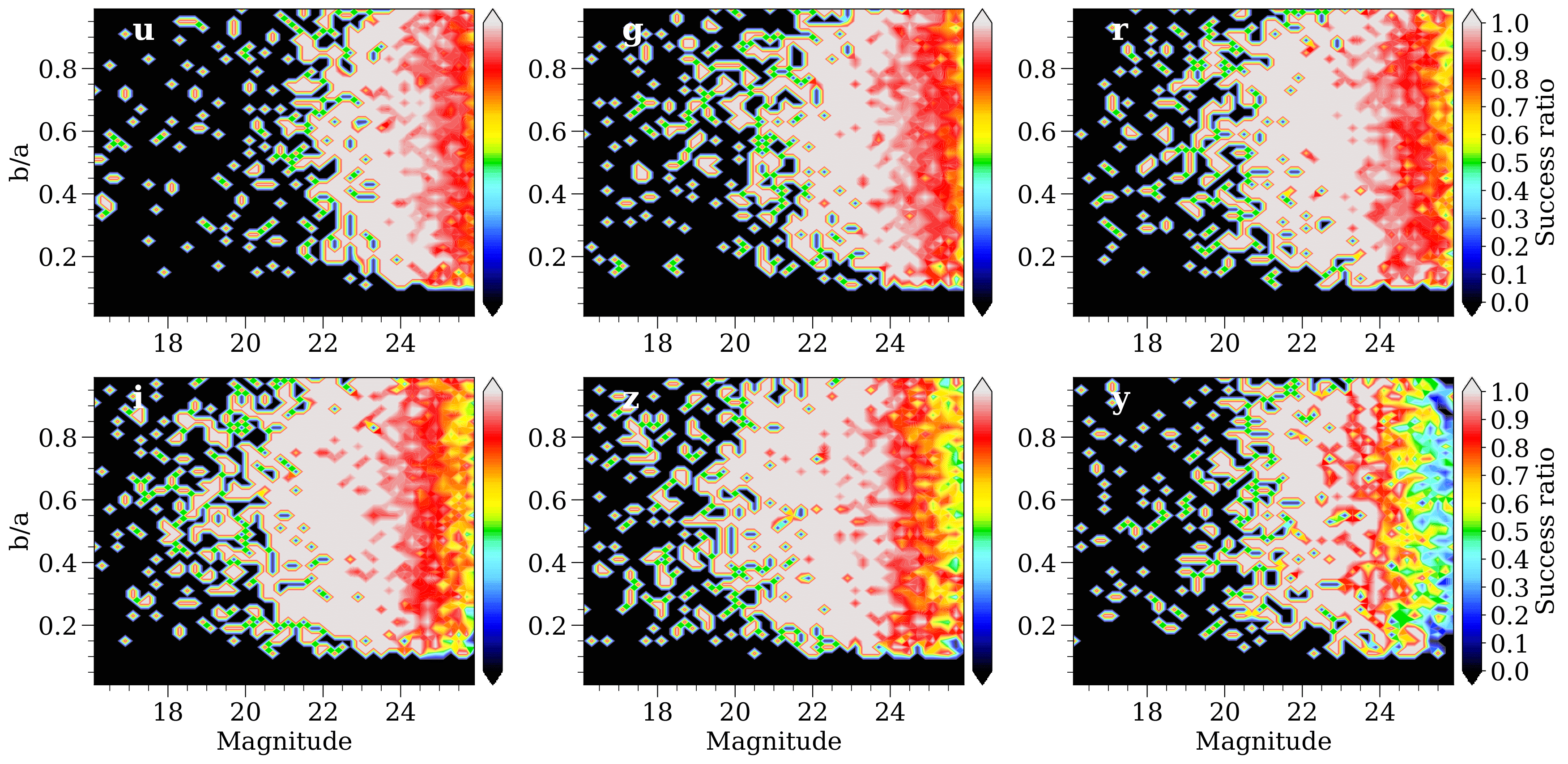
Figure 27: Heat maps showing the simulation success rate (Equation 4) as a function of input magnitude and input axis ratio. Axis ratios of galaxies do not affect the success rate significantly in a given magnitude bin as indicated by the vertical colour stripes.

In Section 3.1, we mention the magnitude limits that we adopt in each band while fitting the light profiles of galaxies. These magnitude limits are as follows: u$<26$; g$<25.5$; r, i, z$<25$. We introduce these limits based on the robustness analysis of our fitting pipeline through the simulations we perform (Section 3.2). We adopt the simulation success rate described in Equation 4 as a proxy for the robustness of the pipeline. This rate tells us what fraction of galaxies with a certain properties we can fit successfully.

Through simulations we investigate how this success rate changes with intrinsic Sérsic parameters of the simulated galaxies. In Figure 7, we show how success rates in each CLAUDS+HSC bands change with the band magnitude of galaxies. It is clear from the figure that the success rate is sensitive to the brightness of a galaxy beyond $24^{\text{th}}$ magnitude in the bands used in this study.

In Figures 25, 26 and 27, we investigate how the success rate depend on other Sérsic parameters - size ($R_{e}$), Sérsic index ($n$) and axis ratio ($b/a$) respectively through heat maps. These figures show the success rate as function of both the input/intrinsic values of these Sérsic parameters and magnitude in a given band. We find that the colours in the heat map in every panel in each figure change horizontally but remain more or less constant vertically. This observed colour pattern in the heat map shows that the success rate and thereby the robustness of the fitting algorithm does not depend on the intrinsic shape of the galaxy ($R_{e}$, $n$ and $b/a$) but the brightness alone. Therefore, we do not adopt any cuts on the data based on $R_{e}$, $n$ and $b/a$.

Appendix B Size-Mass Relation Fitting in Rest-frame UV Light

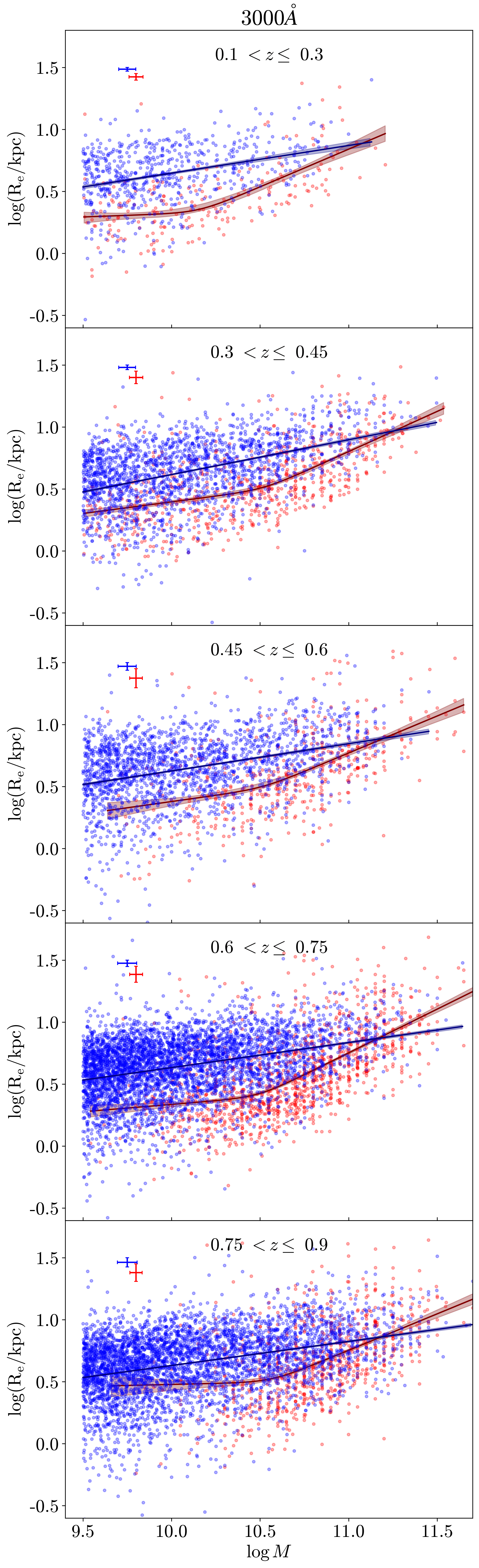
Figure 28: Fitting smoothly broken double power law to the QGs and single power law to the SFGs at rest-frame $3000$ Å in $5$ redshift bins. The individual SFGs are shown as blue points and QGs in red. The median uncertainties in their measurements are given in the top left corner of each panel. The best-fitting power law relations for SFGs and QGs are shown in navy blue and maroon respectively with their uncertainties from Bayesian posterior plotted as shaded region.

In Figure 28, we show the size-mass relation (SMR) for star-forming galaxies (SFGs; blue) and quiescent galaxies (QGs; red) in rest-frame UV light ($3000$ Å). We fit a single power-law for SFGs but a double power-law for QGs initially followed by a single power-law fit for QGs above the pivot mass ($M_{p}$; mass at pivot point) in the double power-law SMR (see Section 4.1). We provide the best-fit parameters of double power-law SMR in Table 4 and single-power law SMR in Table 4.

As we see in Figure 28, the SFGs are on average more extended than QGs in rest-frame UV light in every redshift bin at $0.1<z<0.9$. The SFGs and low mass QGs ($M<M_{p}$) have shallow SMR with an exponent around $0.2$ but the high mass QGs have a steep exponent ($\sim 0.6$). These differences in SFG and QG SMRs are similar to those we find in rest-frame $5000$ Å (see Figure 11).

Appendix C Removing Progenitor Bias from QG Population

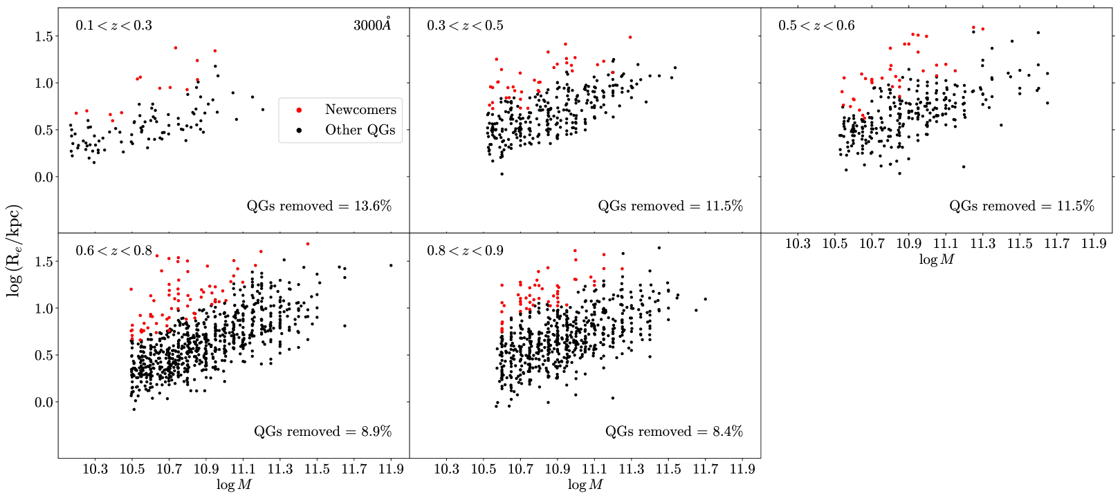
Figure 29: Removing progenitor bias in rest-frame $3000$ Å shown in size-mass plane. We describe the removal process in Section 5.2.2 and Appendix C. The QGs removed (newcomers) are shown in red and the remaining QGs are in black. The percentage of QGs removed are given in each panel.

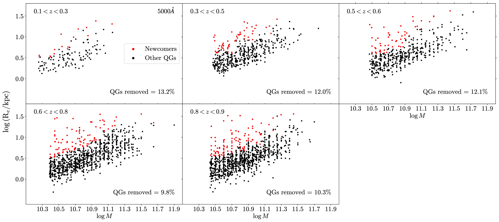
Figure 30: Removing progenitor bias in rest-frame $5000$ Å shown in size-mass plane. As in Figure 29, removed newcomers are in red and other QGs are in black.

Newly quenched galaxies introduces a bias (progenitor bias) when we analyze the size evolution of the quiescent population. Hence, we remove progenitor bias from our QG population as described in Section 5.2.2. In short, we assume that the newly quenched galaxies are more extended than the galaxies those quenched earlier in a given stellar mass bin. We also assume that the quenching efficiency increases with mass and thus, the fraction of newly quenched galaxy in our QG sample varies in stellar mass bins. We estimate this fraction using Equation 14. We normalize this equation so that we remove approximately $10\%$ of QGs from the parent population in each redshift bin.

In Figures 29 and 30 we show the QGs removed in the size-mass plane in rest-frames $3000$ Å and $5000$ Å respectively. In both wavelengths, we remove $8-13\%$ of QGs in each redshift bin and this percentage is given in each panel. The removed QGs (red) are more extended than the remaining QGs in their respective mass bin and their percentage increases towards higher masses by design.

Appendix D Central Stellar Mass Surface Density

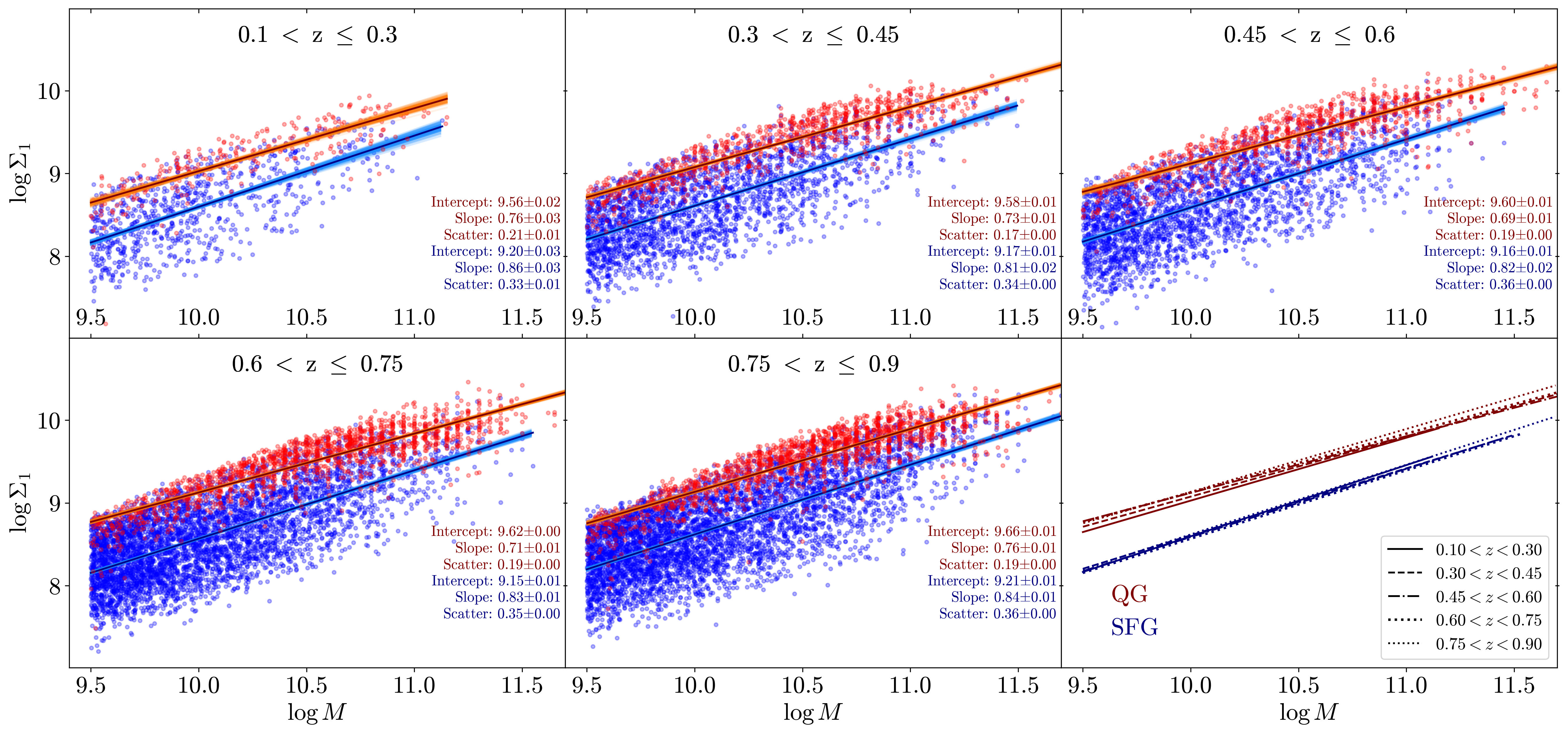
Figure 31: The best-fitting $\log\Sigma_{1}-\log M$ relation for SFGs (blue) and QGs (red) with mass $\log M>9.5$ in $5$ redshift bins. The best-fit single power-law parameters are given in each panel.

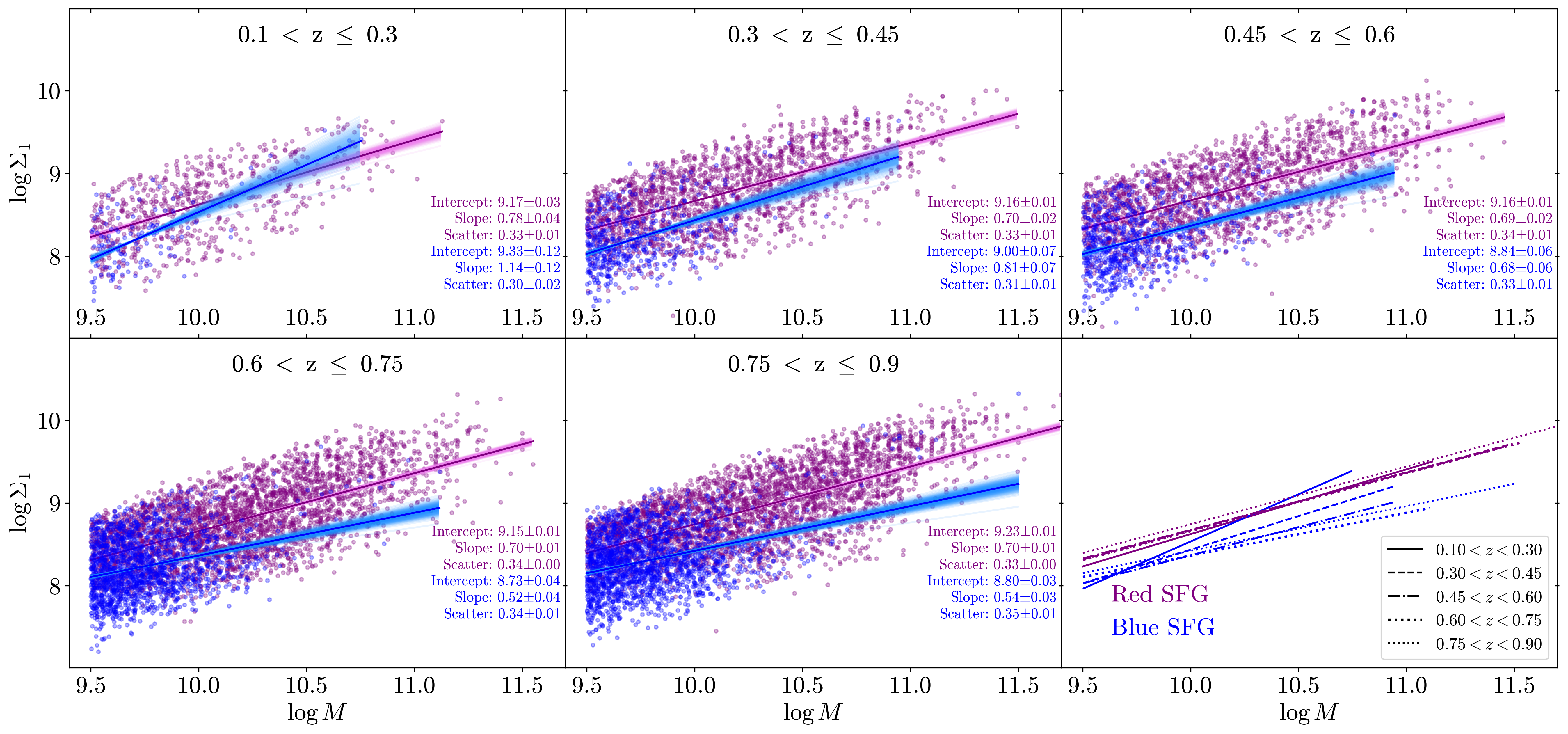
Figure 32: The best-fitting $\log\Sigma_{1}-\log M$ relation for blue and red SFGs (blue and purple colours respectively) with mass $\log M>9.5$ in $5$ redshift bins. The best-fit single power-law parameters are given in each panel.

Following Cheung et al. (2012) and Ji & Giavalisco (2022), we calculate the projected central stellar mass surface density as

$$\Sigma_{1}\left[\frac{\hbox{M${}_{\odot}$}}{\text{kpc}^{2}}\right]=\frac{M_{1\text{kpc}}}{\pi\times 1\text{kpc}^{2}}=\frac{M}{\pi\times 1\text{kpc}^{2}}\frac{\gamma(2n,x)}{\Gamma(2n)},$$ (15)

where $M_{1\text{kpc}}$ is the stellar mass within $1$ kpc radius in M_⊙, $M$ is the total stellar mass in M_⊙, $\gamma$ and $\Gamma$ are incomplete and complete gamma functions, and $x=b_{n}\left(\frac{1\text{kpc}}{R_{e}}\right)^{(1/n)}$. We calculate $b_{n}$ by solving the equation $\Gamma(2n)=2\gamma(2n,b_{n})$ numerically (Graham & Driver, 2005). The caveat here is that we assume a uniform mass-to-light (M/L) ratio within each galaxy. Although this assumption is reasonable for QGs, we acknowledge that the radial variation in $M/L$ ratio is significantly higher for SFG (e.g., Tortora et al., 2011). We attempt to minimize the effect of $M/L$ variation by analyzing the $\Sigma_{1}$ only at the rest-frame $5000$ Å which has more contribution from bulk of the stars (old low-mass stars) than at $3000$ Å. However, even at $5000$ Å, radial variation of $M/L$ ratio can be significant (at least) in SFGs where the overall profile is dominated by the light from young stars in the disks. Hence, the $\Sigma_{1}$ that we estimate are lower limits, especially for SFGs with steep negative colour gradients.

To explore how the characteristic $\Sigma_{1}$ value for SFGs and QGs evolves in Section 5.3, we fit a single power-law to the $\Sigma_{1}$-stellar mass relation in log-log space for SFGs and QGs with mass $\log M>9.5$ in $5$ redshift bins (Figure 31). Across the redshift bins, we do not find any signs of significant evolution in the power-law parameters, in congruence with previous works (e.g., Fang et al. (2013) at $z\sim 0.1$ and Barro et al. (2017) at $0.5<z<3$). The only parameter that we observe changing with time is the zero point for QGs. The $\Sigma_{1}$ of QGs with a characteristic mass $5\times 10^{10}$ M_⊙ increases by $\sim 20\%$ from the lowest to the highest redshift bin.

The $\Sigma_{1}-$stellar mass relation is tighter for QGs than for SFGs (Figure 31). One of the possible reasons for this difference is the strong variation in $M/L$ ratios in SFG radial profiles compared to QG profiles (Tortora et al., 2011). QGs in general have higher $\Sigma_{1}$ than SFGs in any given mass bin and this $\Sigma_{1}$ value is very similar for all QGs with similar stellar mass due to the very tight $\Sigma_{1}-$stellar mass relation. Thus, there exists a threshold $\Sigma_{1}$ value required for a galaxy to be quiescent and this threshold value increases with galaxy stellar mass. It means that forming a dense core is a prerequisite for quenching (or a consequence of quenching) as argued by Cheung et al. (2012), Fang et al. (2013), van Dokkum et al. (2014), Barro et al. (2017), Ji & Giavalisco (2023) and others. However, since some SFGs also have $\Sigma_{1}$ close to the threshold value, having a dense core alone is insufficient for a galaxy to be quiescent.

A lack of evolution in the slopes indicates that the galaxies build up their inner core while they grow in stellar mass in a similar manner across the redshift range. However, $\Sigma_{1}-$stellar mass relation has $15-20\%$ steeper slope for SFGs. This difference in the slopes is at least partially due to the differences in how galaxies evolve before and after quenching. SFGs build up mass more uniformly across the galactocentric radii than QGs. However, we note that the scaling relations for QGs are also affected by recently quenched galaxies (newcomers) through the so-called progenitor bias (Section 5.2.2; Ji & Giavalisco, 2022, 2023).

To further probe the evolution in characteristic $\Sigma_{1}$ for blue and red SGFs separately in Section 5.3, we fit the $\Sigma 1-$stellar mass relations for these two SFG subpopulations in Figure 32. Because the majority of SFGs within our redshift interval is red (purple points in 32; see also Figure 19), the $\Sigma_{1}$ values of the overall SFGs reflect those of red SFGs. The blue SFGs (blue points in 32) generally have lower $\Sigma_{1}$ than red SFGs at a given stellar mass. This suggests that, as blue SFGs turn red, they also build up their central regions.

However, we acknowledge that the parameters of the $\Sigma_{1}-$mass relation for blue SFGs are quite uncertain because of the small sample that covers a narrow dynamic range in stellar masses. At $0.75<z<0.9$, around $45\%$ of SFGs are blue but this percentage drops down to below $15\%$ at $0.1<z<0.3$. Most of these blue SFGs have stellar mass in a narrow $9.5<\log M<10$ interval. Hence, the parameters of the fit for blue SFGs at $z<0.45$, where the fraction of blue galaxies in the star-forming population is below $20\%$, are not well constrained.

References

- Abazajian et al. (2009) Abazajian K. N., et al., 2009, The Astrophysical Journal Supplement Series, 182, 543
- Aihara et al. (2011) Aihara H., et al., 2011, The Astrophysical Journal Supplement Series, 193, 29
- Aihara et al. (2018) Aihara H., et al., 2018, Publications of the Astronomical Society of Japan, 70, S4
- Aihara et al. (2019) Aihara H., et al., 2019, Publications of the Astronomical Society of Japan, 71, 114
- Astropy Collaboration et al. (2013) Astropy Collaboration et al., 2013, Astronomy and Astrophysics, 558, A33
- Astropy Collaboration et al. (2018) Astropy Collaboration et al., 2018, The Astronomical Journal, 156, 123
- Astropy Collaboration et al. (2022) Astropy Collaboration et al., 2022, The Astrophysical Journal, 935, 167
- Athanassoula (2005) Athanassoula E., 2005, Monthly Notices of the Royal Astronomical Society, 358, 1477
- Barden et al. (2005) Barden M., et al., 2005, The Astrophysical Journal, 635, 959
- Barone et al. (2022) Barone T. M., et al., 2022, Monthly Notices of the Royal Astronomical Society, 512, 3828
- Barro et al. (2013) Barro G., et al., 2013, The Astrophysical Journal, 765, 104
- Barro et al. (2014) Barro G., et al., 2014, The Astrophysical Journal, 791, 52
- Barro et al. (2017) Barro G., et al., 2017, The Astrophysical Journal, 840, 47
- Baumgardt & Kroupa (2007) Baumgardt H., Kroupa P., 2007, Monthly Notices of the Royal Astronomical Society, 380, 1589
- Behroozi et al. (2010) Behroozi P. S., Conroy C., Wechsler R. H., 2010, The Astrophysical Journal, 717, 379
- Beifiori et al. (2014) Beifiori A., et al., 2014, The Astrophysical Journal, 789, 92
- Belli et al. (2015) Belli S., Newman A. B., Ellis R. S., 2015, The Astrophysical Journal, 799, 206
- Belli et al. (2017) Belli S., Newman A. B., Ellis R. S., 2017, The Astrophysical Journal, 834, 18
- Belli et al. (2019) Belli S., Newman A. B., Ellis R. S., 2019, The Astrophysical Journal, 874, 17
- Bertin (2011) Bertin E., 2011, in Astronomical Data Analysis Software and Systems XX. p. 435
- Bertin & Arnouts (1996) Bertin E., Arnouts S., 1996, Astronomy and Astrophysics Supplement Series, 117, 393
- Bezanson et al. (2009) Bezanson R., van Dokkum P. G., Tal T., Marchesini D., Kriek M., Franx M., Coppi P., 2009, The Astrophysical Journal, 697, 1290
- Birrer & Amara (2018) Birrer S., Amara A., 2018, Physics of the Dark Universe, 22, 189
- Birrer et al. (2015) Birrer S., Amara A., Refregier A., 2015, The Astrophysical Journal, 813, 102
- Bluck et al. (2012) Bluck A. F. L., Conselice C. J., Buitrago F., Grützbauch R., Hoyos C., Mortlock A., Bauer A. E., 2012, The Astrophysical Journal, 747, 34
- Boecker et al. (2023) Boecker A., Neumayer N., Pillepich A., Frankel N., Ramesh R., Leaman R., Hernquist L., 2023, Monthly Notices of the Royal Astronomical Society, 519, 5202
- Boily & Kroupa (2003) Boily C. M., Kroupa P., 2003, Monthly Notices of the Royal Astronomical Society, 338, 665
- Bosch et al. (2018) Bosch J., et al., 2018, Publications of the Astronomical Society of Japan, 70, S5
- Bower et al. (2006) Bower R. G., Benson A. J., Malbon R., Helly J. C., Frenk C. S., Baugh C. M., Cole S., Lacey C. G., 2006, Monthly Notices of the Royal Astronomical Society, 370, 645
- Boylan-Kolchin et al. (2006) Boylan-Kolchin M., Ma C.-P., Quataert E., 2006, Monthly Notices of the Royal Astronomical Society, 369, 1081
- Bradley et al. (2022) Bradley L., et al., 2022, Zenodo
- Brammer et al. (2008) Brammer G. B., van Dokkum P. G., Coppi P., 2008, The Astrophysical Journal, 686, 1503
- Brammer et al. (2011) Brammer G. B., et al., 2011, The Astrophysical Journal, 739, 24
- Breda et al. (2020) Breda I., et al., 2020, Astronomy and Astrophysics, 635, A177
- Bruzual & Charlot (2003) Bruzual G., Charlot S., 2003, Monthly Notices of the Royal Astronomical Society, 344, 1000
- Buitrago et al. (2017) Buitrago F., Trujillo I., Curtis-Lake E., Montes M., Cooper A. P., Bruce V. A., Pérez-González P. G., Cirasuolo M., 2017, Monthly Notices of the Royal Astronomical Society, 466, 4888
- Bundy et al. (2009) Bundy K., Fukugita M., Ellis R. S., Targett T. A., Belli S., Kodama T., 2009, The Astrophysical Journal, 697, 1369
- Carnall et al. (2018) Carnall A. C., McLure R. J., Dunlop J. S., Davé R., 2018, Monthly Notices of the Royal Astronomical Society, 480, 4379
- Carollo et al. (2013) Carollo C. M., et al., 2013, The Astrophysical Journal, 773, 112
- Carollo et al. (2016) Carollo C. M., et al., 2016, The Astrophysical Journal, 818, 180
- Ceverino et al. (2010) Ceverino D., Dekel A., Bournaud F., 2010, Monthly Notices of the Royal Astronomical Society, 404, 2151
- Chen et al. (2020) Chen Z., et al., 2020, The Astrophysical Journal, 897, 102
- Cheung et al. (2012) Cheung E., et al., 2012, The Astrophysical Journal, 760, 131
- Christlein & Zabludoff (2004) Christlein D., Zabludoff A. I., 2004, The Astrophysical Journal, 616, 192
- Cimatti et al. (2012) Cimatti A., Nipoti C., Cassata P., 2012, Monthly Notices of the Royal Astronomical Society, 422, L62
- Collaboration et al. (2022) Collaboration E., et al., 2022, Astronomy and Astrophysics, 658, A126
- Conroy (2013) Conroy C., 2013, Annual Review of Astronomy and Astrophysics, 51, 393
- Conselice (2014) Conselice C. J., 2014, Annual Review of Astronomy and Astrophysics, 52, 291
- Conselice et al. (2003) Conselice C. J., Bershady M. A., Dickinson M., Papovich C., 2003, The Astronomical Journal, 126, 1183
- Conselice et al. (2022) Conselice C. J., Mundy C. J., Ferreira L., Duncan K., 2022, The Astrophysical Journal, 940, 168
- Croton et al. (2006) Croton D. J., et al., 2006, Monthly Notices of the Royal Astronomical Society, 365, 11
- Damjanov et al. (2009) Damjanov I., et al., 2009, The Astrophysical Journal, 695, 101
- Damjanov et al. (2011) Damjanov I., et al., 2011, The Astrophysical Journal, 739, L44
- Damjanov et al. (2019) Damjanov I., Zahid H. J., Geller M. J., Utsumi Y., Sohn J., Souchereau H., 2019, The Astrophysical Journal, 872, 91
- Damjanov et al. (2023) Damjanov I., Sohn J., Geller M. J., Utsumi Y., Dell’Antonio I., 2023, The Astrophysical Journal, 943, 149
- Danovich et al. (2015) Danovich M., Dekel A., Hahn O., Ceverino D., Primack J., 2015, Monthly Notices of the Royal Astronomical Society, 449, 2087
- Dekel et al. (2009) Dekel A., Sari R., Ceverino D., 2009, The Astrophysical Journal, 703, 785
- Desprez et al. (2023) Desprez G., et al., 2023, A&A, 670, A82
- Dey et al. (2019) Dey A., et al., 2019, The Astronomical Journal, 157, 168
- Driver & Robotham (2010) Driver S. P., Robotham A. S. G., 2010, Monthly Notices of the Royal Astronomical Society, 407, 2131
- Driver et al. (2007) Driver S. P., Popescu C. C., Tuffs R. J., Liske J., Graham A. W., Allen P. D., de Propris R., 2007, Monthly Notices of the Royal Astronomical Society, 379, 1022
- Dutton (2009) Dutton A. A., 2009, Monthly Notices of the Royal Astronomical Society, 396, 121
- Estrada-Carpenter et al. (2023) Estrada-Carpenter V., et al., 2023, The Astrophysical Journal, 951, 115
- Fagioli et al. (2016) Fagioli M., Carollo C. M., Renzini A., Lilly S. J., Onodera M., Tacchella S., 2016, The Astrophysical Journal, 831, 173
- Faisst et al. (2017) Faisst A. L., Carollo C. M., Capak P. L., Tacchella S., Renzini A., Ilbert O., McCracken H. J., Scoville N. Z., 2017, The Astrophysical Journal, 839, 71
- Fan et al. (2008) Fan L., Lapi A., De Zotti G., Danese L., 2008, The Astrophysical Journal, 689, L101
- Fan et al. (2010) Fan L., Lapi A., Bressan A., Bernardi M., De Zotti G., Danese L., 2010, The Astrophysical Journal, 718, 1460
- Fang et al. (2013) Fang J. J., Faber S. M., Koo D. C., Dekel A., 2013, The Astrophysical Journal, 776, 63
- Foster et al. (2012) Foster C., et al., 2012, A&A, 547, A79
- Franx et al. (2008) Franx M., van Dokkum P. G., Förster Schreiber N. M., Wuyts S., Labbé I., Toft S., 2008, The Astrophysical Journal, 688, 770
- Gabrielpillai et al. (2022) Gabrielpillai A., Somerville R. S., Genel S., Rodriguez-Gomez V., Pandya V., Yung L. Y. A., Hernquist L., 2022, Monthly Notices of the Royal Astronomical Society, 517, 6091
- Gadotti (2009) Gadotti D. A., 2009, Monthly Notices of the Royal Astronomical Society, 393, 1531
- Genel et al. (2018) Genel S., et al., 2018, Monthly Notices of the Royal Astronomical Society, 474, 3976
- Golden-Marx & Miller (2019) Golden-Marx J. B., Miller C. J., 2019, The Astrophysical Journal, 878, 14
- Golden-Marx et al. (2022) Golden-Marx J. B., et al., 2022, The Astrophysical Journal, 928, 28
- Goodwin & Bastian (2006) Goodwin S. P., Bastian N., 2006, Monthly Notices of the Royal Astronomical Society, 373, 752
- Graham & Driver (2005) Graham A. W., Driver S. P., 2005, Publications of the Astronomical Society of Australia, 22, 118
- Guo et al. (2009) Guo Y., et al., 2009, Monthly Notices of the Royal Astronomical Society, 398, 1129
- Guo et al. (2021) Guo Y., et al., 2021, The Astrophysical Journal, 914, 7
- Gustafsson (1989) Gustafsson B., 1989, Annual Review of Astronomy and Astrophysics, 27, 701
- Hamadouche et al. (2022) Hamadouche M. L., et al., 2022, Monthly Notices of the Royal Astronomical Society, 512, 1262
- Harris et al. (2020) Harris C. R., et al., 2020, Nature, 585, 357
- Hashemizadeh et al. (2022) Hashemizadeh A., et al., 2022, Monthly Notices of the Royal Astronomical Society, 515, 1175
- Hilz et al. (2012) Hilz M., Naab T., Ostriker J. P., Thomas J., Burkert A., Jesseit R., 2012, Monthly Notices of the Royal Astronomical Society, 425, 3119
- Hopkins et al. (2009) Hopkins P. F., Bundy K., Murray N., Quataert E., Lauer T. R., Ma C.-P., 2009, Monthly Notices of the Royal Astronomical Society, 398, 898
- Hopkins et al. (2010) Hopkins P. F., et al., 2010, The Astrophysical Journal, 715, 202
- Huang et al. (2017) Huang K.-H., et al., 2017, The Astrophysical Journal, 838, 6
- Hudson et al. (2010) Hudson M. J., Stevenson J. B., Smith R. J., Wegner G. A., Lucey J. R., Simard L., 2010, Monthly Notices of the Royal Astronomical Society, 409, 405
- Huertas-Company et al. (2013) Huertas-Company M., et al., 2013, Monthly Notices of the Royal Astronomical Society, 428, 1715
- Hunter (2007) Hunter J. D., 2007, Computing in Science and Engineering, 9, 90
- Huško et al. (2022) Huško F., Lacey C. G., Baugh C. M., 2022, Monthly Notices of the Royal Astronomical Society, 509, 5918
- Huško et al. (2023) Huško F., Lacey C. G., Baugh C. M., 2023, Monthly Notices of the Royal Astronomical Society, 518, 5323
- Ilbert et al. (2006) Ilbert O., et al., 2006, Astronomy and Astrophysics, 457, 841
- Inoue et al. (2016) Inoue S., Dekel A., Mandelker N., Ceverino D., Bournaud F., Primack J., 2016, Monthly Notices of the Royal Astronomical Society, 456, 2052
- Ji & Giavalisco (2022) Ji Z., Giavalisco M., 2022, The Astrophysical Journal, 935, 120
- Ji & Giavalisco (2023) Ji Z., Giavalisco M., 2023, The Astrophysical Journal, 943, 54
- Ji et al. (2020) Ji Z., et al., 2020, ApJ, 888, 109
- Ji et al. (2022) Ji Z., Giavalisco M., Kirkpatrick A., Kocevski D., Daddi E., Delvecchio I., Hatcher C., 2022, ApJ, 925, 74
- Kaviraj et al. (2014) Kaviraj S., et al., 2014, Monthly Notices of the Royal Astronomical Society, 443, 1861