Optimization of Discrete Parameters Using the Adaptive Gradient Method and Directed Evolution

Abstract

The problem is considered of optimizing discrete parameters in the presence of constraints. We use the stochastic sigmoid with temperature and put forward the new adaptive gradient method CONGA. The search for an optimal solution is carried out by a population of individuals. Each of them varies according to gradients of the ’environment’ and is characterized by two temperature parameters with different annealing schedules. Unadapted individuals die, and optimal ones interbreed, the result is directed evolutionary dynamics. The proposed method is illustrated using the well-known combinatorial problem for optimal packing of a backpack (0–1 KP).

1 Introduction

Deep learning models usually utilize real-valued parameters. This is due to the fact that the only known optimization method applicable to models with millions or more parameters is gradient descent. However, many tasks that machine learning is aiming to solve are intrinsically discrete in nature. This discreteness may follow directly from the structure of the input or output data, and also can be optimal configuration for the latent feature space.

For example, natural language operates with tokens, the relationship between which can be described using tree structures. A similar situation occurs when working with particles, molecules, graphs and other objects that are of a discrete nature. Over the years, researchers have become adept at ’encoding’ discrete objects using continuous parameters (using embedding vectors, for example). However, this accomplishment comes at the cost of introducing a large number of redundant parameters.

There are numerous real world problems that require a solution of optimization task with constrained parameters, some of the most prominent examples being the traveling salesman problem (TSP), ranking and sorting algorithms, routing optimization, the 0–1 knapsack problem, and many other. Application to these combinatorial problems of the traditional ML methods that rely on the gradient descent is not straightforward, as the solution space is discrete and objective functions are not differentiable, as they involve step-wise decisions or discrete choices, rendering gradients undefined or impractical to compute. Also traditional gradient-based methods may not naturally integrate constraint satisfaction into the optimization process. Researchers put forward a number of approaches to tackle these difficulties. After the papers [1, 2, 3] introduced the continuous relaxation of discrete random variables it became possible to use the gradient method for discrete parameters.

In the present paper we put forward a new adaptive gradient method for discrete optimization tasks. The layout of the paper is as follows. In Section 2 we give a brief overview of the research conducted recently in the domain of discrete optimization problems with constraints. Section 3 presents our new method for solving such problems, CONstrained Gradient descent with Adaptation (CONGA). The application of hot and stochastic sigmoids for gradient computation is discussed in detail; the optimization procedure is carried out by a population of individuals in directed dynamic evolution. Section 4 demonstrates the performance of the CONGA method applied to one of the benchmark discrete problems, the 0–1 Knapsack Problem. The numerical details of the experiments and comparison of our results to branch and bound, genetic algorithm, greedy search algorithm and simulated annealing are compiled in the Appendices.

2 Related Work

In [1] a multi-scale approach was proposed, called the hierarchical multi-scale recurrent neural network, that can capture the latent hierarchical structure in the sequence by encoding the temporal dependencies with different timescales. It found that the straight-through estimator is one efficient way of training a model containing discrete variables is the straight-through estimator, which was first introduced in [4] and works by decomposing the operation of a binary stochastic neuron into a stochastic binary part and a smooth differentiable part, approximating the expected effect of the pure stochastic binary neuron.

Authors of [2] introduced the continuous relaxation of discrete random variables, using Gumbel-Softmax trick. They introduce the Concrete distribution with a closed form density parameterized by a positive temperature parameter. The essence of the approach is that the zero temperature limit of a Concrete distribution corresponds to a discrete distribution of parameters. Thus, optimization of an objective over an architecture with discrete stochastic nodes can be accomplished by gradient descent on the samples of the corresponding continuous relaxation.

The concept of employing a Gumbel-Softmax as a relaxation technique for discrete random variables was also explored by [3]. In their approach, the relaxed objective does not incorporate density; rather, all elements of the graph are evaluated using the relaxed stochastic state of the graph, which includes discrete log-probability calculations. Gumbel-Softmax estimator outperformed gradient estimators on both Bernoulli variables and categorical variables; the most important result is a differentiable approximate sampling mechanism for categorical variables that can be integrated into neural networks and trained using standard backpropagation. A recent survey of the applications of Gumbert-softmax trick to numerous machine learning tasks, as well as its extensions and modifications is available in [5].

There are a wide range of machine learning problems and applications, where discrete optimization may be profitably applied. We will outline here some interesting examples of recent research in the field. Vector quantized variational autoencoders (VAE) were first introduced in [6]; the approach uses discrete rather than continuous latent space of categorical variables, which is arguably better corresponds to many language tasks. Another discretization of the VAE was considered in [7] for the task of text-to-image generation (the first incarnation of DALL-E); this paper implements the autoregressive transformer model and utilizes the Gumbel-Softmax optimization.

In the paper [8] authors proposed using VAE for a masked image modeling task to pretrain vision transformers (BEiT) in a self-supervised manner; this self-supervised model learned to segment semantic regions and object boundaries without prior human annotation.

Another productive family of models for the discrete optimization are graph neural networks. MolGAN [9] is a generative model for small molecular graphs that circumvents the need for expensive graph matching procedures or node ordering heuristics, adapting instead generative adversarial networks (GANs) to operate directly on graph-structured data, in combination with a reinforcement learning, and generate molecules with specific desired chemical properties.

The medical Generative Adversarial Network (medGAN) introduced in [10] can generate realistic synthetic high-dimensional patient records, containing discrete variables (e.g., binary and count features) via a combination of an autoencoder and generative adversarial networks.

Sorting and ranking of the input objects is a key step in many algorithms and an important task in itself (e.g. ranking the documents in web or database search). The Gumbel-Sinkhorn algorithm, an analog of Gumbel-Softmax for permutations, was constructed in [11] and applied to several diverse problems (number sorting, jigsaw puzzle solving, identifying C. elegans neural signals), outperforming state-of-the-art neural network baselines. Recently proposed Sparse Sinkhorn Attention [12] is a new memory-efficient method for learning to attend, based on differentiable sorting of internal representations for transformer networks. This approach learns to generate latent permutations over sequences, and with sorted sequences, is able to compute global attention with only local windows, mitigating the memory constraints.

Let’s us now turn to 0–1 Knapsack Problem (KP) [13], a classic NP-hard problem that is frequently encountered in real-world scenarios, including decision-making processes, resource allocation, cryptography, and computer vision. It involves selecting the best combination of items to maximize an objective function while satisfying a certain budget constraint. Over time, numerous algorithms have been devised to efficiently solve the KP. While some rely on traditional combinatorial optimization techniques, others harness the power of deep learning methods. Traditional methods such as integer linear programming and dynamic programming provide exact solutions but often suffer from scalability issues. As the dimensionality of the problem increases, the runtime of classical algorithms tends to grow exponentially, which can be a significant drawback in practical applications. Even for the relatively low-dimensional KP there are classes of instances that pose serious difficulties for the exact methods, as was shown in [14]. Here, several instance dataset generation algorithms were constructed, which were later used by many researchers to produce the benchmarks for consistent comparison of the results. Several new computationally challenging problems were recently described in [15].

A comparative study of meta-heuristic optimization algorithms for 0–1 KP is given in [16, 17, 18], which provide a theoretical review and experimental results of applying a number of methods, including genetic algorithms, simulated annealing, branch and bound, dynamic programming, and greedy search algorithm. In recent years, a number of attempts were made at solving the combinatorial optimization problems by deep learning methods. For example, the traveling salesman problem is being solved by recurrent neural networks in [19]. A machine learning approach to getting an approximate solution to the KP is proposed in the paper [20], consisting in randomly generating of large quantity of samples of 0–1 KP and applying supervised learning to train a pointer network to this task. Another novel method to solve the large-scale hard KPs using advanced deep learning techniques was proposed in [21]. The authors designed an adaptive gradient descent method that proved able to optimize the KP objective function, and conducted extensive experiments with state-of-the-art baseline methods and benchmark KP datasets.

3 Proposed Method

Let’s consider the problem of maximizing the function $v(\mathbf{x})>0$ of binary variables $\mathbf{x}=\{x_{1},...,x_{n}\}$ in the presence of a constraint:

$$v(\mathbf{x})=\max,\leavevmode\nobreak\ \leavevmode\nobreak\ \leavevmode\nobreak\ \leavevmode\nobreak\ \leavevmode\nobreak\ \leavevmode\nobreak\ w(\mathbf{x})\leq 0,\leavevmode\nobreak\ \leavevmode\nobreak\ \leavevmode\nobreak\ \leavevmode\nobreak\ \leavevmode\nobreak\ \leavevmode\nobreak\ x_{k}\in\{0,1\}.$$ (1)

Using the gradient method $\mathbf{x}\mapsto\mathbf{x}-\lambda\nabla L$ with learning rate $\lambda$, we will look for the minimum of the following loss function:

$$L(\mathbf{x})=-v(\mathbf{x})+\frac{\gamma}{\nu}\,\bigr{[}\max(0,w(\mathbf{x}))\bigr{]}^{\nu},$$ (2)

where $\gamma\geq 0$, $\nu>0$ are hyperparameters that determine the magnitude of the penalty for violating the constraint $w(\mathbf{x})\leq 0$. In the paper [21], a ’game-theoretic approach’ was used to justify the choice of $\nu=2$, which resulted from the use of the quadratic regularization term. In general, the choice of $\nu$ is arbitrary and depends on the nature of the function $w(\mathbf{x})$. For smooth functions, it is reasonable to set $\nu>1$ so that there is no gradient jump at the transition point from the allowed region $w(\mathbf{x})\geq 0$ to the forbidden one $w(\mathbf{x})<0$ and back.

3.1 The Hot Sigmoid

We cannot directly minimize the loss function $L(\mathbf{x})$ using the gradient method because the derivatives by the integer-valued variables $x_{k}$ are not defined.

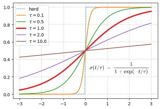
Figure 1: Heaviside function (dashed) and sigmoid for different values of temperature $\tau$

We thus will compute the error gradient using the real-valued variable $t\in[-\infty,\infty]$ (the last letter in the word logit). The Heaviside function $x=H(t)$ of the logit is equal to $x=1$ (for $t>0$) and $x=0$ otherwise (in the graph 1 $H(t)$ is shown by the dashed line, while the logit $t$ is plotted on the horizontal axis).

After substituting $x_{k}=H(t_{k})$ into $L(\mathbf{x})$, we see the loss now depends on the continuous parameters $t=\{t_{1},...,t_{n}\}$, still only taking on the ’allowed values’ since $x_{k}$ are still discrete quantities. However, the derivative of $H(t)$ at $t\neq 0$ is zero. Hence, the error gradient will also vanish.

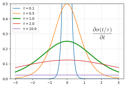
Figure 2: The derivative of the sigmoid with temperature at different values of $\tau$

To solve this problem, following the [1], we will do the following. In the forward pass (when $L$ is computed), we will use the Heaviside function to obtain $x_{k}$. In the backward pass (when computing the gradient $\nabla L$), we will assume that $x_{k}$ was obtained using a hot sigmoid with temperature $\tau$ (the ’smooth Heaviside function’). Figure 1 shows the shape of this function for different values of temperature $\tau$, and Figure 2 shows its derivative. The closer $\tau$ is to zero, the more closely the sigmoid fits the stepped Heaviside function. In fact, the following rule is used:

$$x=H(t),\leavevmode\nobreak\ \leavevmode\nobreak\ \leavevmode\nobreak\ \leavevmode\nobreak\ \leavevmode\nobreak\ \leavevmode\nobreak\ \leavevmode\nobreak\ \leavevmode\nobreak\ \leavevmode\nobreak\ \leavevmode\nobreak\ \leavevmode\nobreak\ \leavevmode\nobreak\ \leavevmode\nobreak\ \leavevmode\nobreak\ \frac{\partial x}{\partial t}=\frac{\partial\sigma(t/\tau)}{\partial t}.$$ (3)

During the training the temperature is usually assumed to be high $\tau\geq 1$ at first and the derivatives of discrete $x_{k}$ by the logits $t_{k}$ will be different from zero (while $x_{k}$ remains discrete). As the temperature gradually decreases, the derivatives outside the region $t\sim 0$ decrease, but they nevertheless ’steer’ the values of the discrete parameters $x_{k}$ to their optimal values. The software implementation of this computation is discussed in Appendix A.

3.2 The Stochastic Sigmoid

It is often convenient to consider the binary parameter $x\in\{0,1\}$ as a random variable that takes the value 1 with probability $p$ and 0 with probability $1-p$. This nondeterminism helps to get out of local minima, and in supervised learning tasks leads to data augmentation, thus reducing overfitting.

To construct a stochastic estimator of the discrete value $x$ from the real logit $t$, let us use the logistic probability distribution $\mathcal{L}(0,s)$:

$$f(t)=\frac{e^{-t/s}}{(1+e^{-t/s})^{2}},\leavevmode\nobreak\ \leavevmode\nobreak\ \leavevmode\nobreak\ \leavevmode\nobreak\ \leavevmode\nobreak\ \leavevmode\nobreak\ \leavevmode\nobreak\ \leavevmode\nobreak\ \leavevmode\nobreak\ \leavevmode\nobreak\ \leavevmode\nobreak\ \leavevmode\nobreak\ \leavevmode\nobreak\ F(t)=\int\limits^{t}_{-\infty}f(z)\,dz=\sigma(t/s),$$ (4)

where $f(t)$ is the probability density function, $F(t)$ is the probability distribution, and $s$ is a parameter characterizing the dispersion of the random variable.

The probability that the random variable $\varepsilon\sim\mathcal{L}(0,s)$ is less than given $t$, is by definition equal to $P(\varepsilon<t)=F(t)=\sigma(t/s)$. This means that with probability $\sigma(t/s)$ the value of $t-\varepsilon$ is positive (the probability density $f(t)$ is symmetric and $\varepsilon$ can be both subtracted and added to $t$). Therefore, if one subtracts $\varepsilon\sim\mathcal{L}(0,s)$ from the logit in a deterministic sigmoid with temperature and computes the Heaviside function from the result, then with probability $\sigma(t/s)$ one will obtain 1, and 0 otherwise:

$$\varepsilon\sim\mathcal{L}(0,s)\leavevmode\nobreak\ \leavevmode\nobreak\ \leavevmode\nobreak\ \Rightarrow\leavevmode\nobreak\ \leavevmode\nobreak\ \leavevmode\nobreak\ H(t-\varepsilon)=\left\{\begin{array}[]{lll}1&\text{with probability}&\sigma(t/s)\\ 0&\text{otherwise}\end{array}\right.$$ (5)

Note also that the logistic distribution is a limiting case of the Gumbel distribution ([2], [3]) when dealing with a categorical variable that has only two values.

The value of the parameter $s$ depends on the problem we are trying to solve. We can set $s=1$; then for the temperature annealing (decreasing $\tau$) the stochasticity will decrease only if the absolute values of logits grow large during the training. For some problems, the ’stochasticity with heating’ is more appropriate, where $s$ is minimal at the beginning of training, then increases to a maximum value and decreases towards the end of training.

As a result, we have two ’temperatures’ with different annealing schedules. One temperature ($\tau$) regulates the transition from continuous variable space to discrete, and the second one ($s$) regulates the degree of random variability of the parameters.

3.3 CONGA - CONstrained Gradient descent with Adaptation

The optimization problem in the presence of constraints leads to the loss function (2) with a cusp (the penalty is zero when $w(\mathbf{x})\geq 0$, and different from zero otherwise). One problem in applying the gradient method to such loss function is related to the choice of the parameter $\gamma$. If it is small, the penalty may be insufficient and the minimum point will be located in the forbidden region $w(\mathbf{x})>0$. When $\gamma$ is large, the solution on the boundary of the region starts to experience oscillations, which slows down convergence. The problem is partially solved if we apply the exponential moving average (EMA) smoothing to the gradients. Nevertheless, it would be advantageous to have a method that selects the optimal value of the hyperparameter $\gamma$. In what follows, we will put forward such a method.

Following [21] we require that in the next step of the gradient method the positive penalty for violating the constraint decreases: $w(\mathbf{x}-\lambda\,\nabla L)=(1-\mu)\,w(\mathbf{x})$. This leads to a new adaptive method to select the parameter $\gamma$, which we have named CONGA (CONstrained Gradient descent with Adaptation):

$$\gamma=\frac{\nabla v\nabla w+\mu\,w}{w^{\nu-1}\,(\nabla w)^{2}},\leavevmode\nobreak\ \leavevmode\nobreak\ \leavevmode\nobreak\ \leavevmode\nobreak\ \leavevmode\nobreak\ \leavevmode\nobreak\ \gamma=\max(0,\,\gamma),$$ (6)

In fact, instead of the hyperparameter $\gamma$, another one $\mu\in[0...1]$ is introduced. It is worth pointing out that unlike $\gamma$, this new parameter has the simple meaning and the corresponding rule to select its value: the target relative reduction of the violation of the constraint condition $w(\mathbf{x})$ at the next step of the gradient method. Additionally, we introduce the parameters $\beta_{v},\leavevmode\nobreak\ \beta_{w}\in[0...1]$ of EMA smoothing of gradients $\nabla v$ and $\nabla w$ using them in (6) and in the loss-function gradient $\nabla L$. Details of the computations and comparisons with the adaptive method of [21] are given in the Appendix B.

3.4 The Population of Solutions

Using the GPU one can efficiently calculate the functions $v(\mathbf{x})$, $w(\mathbf{x})$ and their gradients simultaneously for several trajectories in the parameter space. In our experiments, we create $m$ ’individuals’ with logits $\mathbf{t}^{(k)}$, $k=1,...,m$, which have different initial positions. These vectors are independently and simultaneously varied according to the CONGA method.

In addition to the ’innate’ (initial) diversity, individuals have different values of the hyperparameter $\mu$. As experiments have shown, the hyperparameter $\mu$ for each example has its own value at which the given problem better converges to the optimal solution. Therefore, one of the tasks of a population of ’individuals’ is to choose the optimal distribution of a given hyperparameter. The lifetime of a population of individuals is limited by another hyperparameter (epochs), after this interval the selection of ’individuals’ is performed in the following way. The best ’individuals’ (top 20%) are selected that have the largest maximum backpack value. The range of parameter $\mu_{best}\in[\mu_{min},\mu_{max}]$ is determined for these solutions, and then the range boundaries are proportionally expanded: $\mu_{next}\in[\mu_{min}/frac,\mu_{max}\cdot frac]$. The resulting range is used to create new ’individuals’ of the population. As the result, the directed evolutionary dynamics is obtained.

Algorithm 1 CONGA

$gen\_id=0$

for all n_generations do

      if $gen\_id>0$ then

           $p_{k}=selection(p_{k-1})$ $\triangleright$ selecting top individuals from generation

      else

           $p_{k}\leftarrow$ individual

      end if

      for all epochs do

           for all individual do

                 $x_{k}=hot\_sigmoid(p_{k})$ $\triangleright$ soft/hard sigmoid

                 $v_{k}=v(\mathbf{x}_{k})$

                 $w_{k}=w(\mathbf{x}_{k})$

                 $\mathbf{V}_{k}\leavevmode\nobreak\ \leftarrow\beta_{v}\,\mathbf{V}_{k}\leavevmode\nobreak\ \,+(1-\beta_{v})\nabla v(\mathbf{x}_{k})$ $\triangleright$ gradient smoothing

                 $\mathbf{W}_{k}\leftarrow\beta_{w}\,\mathbf{W}_{k}+(1-\beta_{w})\nabla w(\mathbf{x}_{k})$

                 $\gamma_{k}=\max(0,\leavevmode\nobreak\ (\mathbf{V}_{k}\mathbf{W}_{k}+\mu\,w_{k}/\lambda)/(w^{\nu-1}_{k}\,\mathbf{W}^{2}_{k})\,)$

                 $\mathbf{p}_{k+1}\leftarrow\mathbf{p}_{k}-\lambda\,(-\mathbf{V}_{k}+\gamma_{k}\,\max(0,w_{k})^{\nu-1}\,W_{k})$

           end for

      end for

end for

4 Experimental Results

We will demonstrate the performance of the CONGA method using the dataset for 0–1 Knapsack Problem described in [22]. The dataset is split into groups depending on the number of items and the correlation of values and their weights as shown in the table 1. The following hardware platform was used in the experiments: Intel(R) Xeon(R) 2.00GHz CPU, Tesla T4 GPU. The source code is implemented in Python and is available online in the repository at https://github.com/QuDataAI/CONGA.

Table 1: Datasets.

[1.2pt] name	items	correlation	tasks
[1.2pt] LD-UC	4-20	uncorrelated	10
[1pt] HD-UC	100-10000	uncorrelated	7
[1pt] HD-WC	100-10000	weakly correlated	7
[1pt] HD-SC	100-10000	strongly correlated	7
[1.2pt]

4.1 Single-Agent Case

Let us now consider the application of this method without directed evolution in the mode with only one agent. For this case, the number of populations and the number of agents are $n\_generations=1,n\_agents=1$.

The agent, having received the task, initializes the initial state of the backpack packing vector randomly with a normal distribution. Then, using the CONGA method, the value of the backpack is iteratively optimized while changing the packing vector and taking into account the weight constraint. The maximum number of such iterations is limited by the hyperparameter $epochs=2000$ in order to prevent an infinite search for the optimal solution.

As a result of optimization, the agent can come to either an exact or an approximate solution, however the iteration always converges to a valid solution.

To evaluate the results we will use the following metrics:

$$acc=\frac{1}{n}\sum_{i=1}^{n}(v_{opt}==v),\leavevmode\nobreak\ \leavevmode\nobreak\ \leavevmode\nobreak\ \leavevmode\nobreak\ \leavevmode\nobreak\ time=\frac{1}{n}\sum_{i=1}^{n}t$$ (7)

where $v_{opt}$ is the optimal value of the backpack, $v$ is the value of the backpack after optimization, $n$ is the number of tasks in the dataset, $t$ is the time to solve one problem in seconds. Thus, $acc$ shows how many problems reached the optimal solution, and $time$ is the average time to solve one problem in seconds.

By running this experiment, we obtained the following metrics: $\{acc:0.48,\leavevmode\nobreak\ \leavevmode\nobreak\ time:2.655\}$, therefore, we solve optimally less than half of the problems, while spending approximately 3 seconds on each problem.

Figure 3: Single-agent accuracy for different task types

The outcome of the optimizer application to different types of problems is presented in Fig. 3. As one can see, the method works better with a dataset in which there are fewer objects, but one agent is clearly not enough to solve more complex problems.

4.2 Multi-Agent Case

The multi-agent approach allows one to solve the problem in parallel by several agents, as representatives of the population that has a common goal, but each agent has a unique initial state of the backpack packing vector. Thanks to GPU parallelization, we can significantly increase the number of agents without losing processing speed.

We can see how the optimizer’s result changes depending on the number of agents in Fig. 4.

Figure 4: Metric $acc$ dependence on the number of agents

Figure 5: Dependence of the mean solution time on the number of agents

As one can see, 50 agents is optimal for solving problems, and yields the metric values equal to $\{acc:0.74(+0.26),\leavevmode\nobreak\ \leavevmode\nobreak\ time:2.964(+0.309)\}$, while the average time spent on solving one problem increased by only $309ms$ thanks to parallel computing on the GPU.

A further increase in the number of agents linearly increases the time to process one task as shown in Fig. 5, but the result does not improve. Thus, we fix the hyperparameter $n\_agents=50$

4.3 Directed Evolutionary Dynamics

Analyzing the process of solving problems in the dataset, we noticed that some problems are successfully solved with small values of the parameter $\mu$ from Eq. 6, while others require higher values as shown in the histogram 6.

Figure 6: Histogram of parameter density $\mu$ among optimal solutions

Therefore, we proceeded to endow our method with the properties of a genetic algorithm. Agents from the population randomly select a hyperparameter value $\mu$ from the range $[0.2,8.0]$. After reaching the maximum number of epochs, agents with the best backpack values are selected. As a result of selection, we determine a new hyperparameter range $\mu$ that better optimizes this problem. Then we create a new population of agents that inherit the updated range $\mu$ and therefore optimize the solution based on the experience of their ancestors. The number of such iterations is determined by the hyperparameter $n\_generations$.

Executing such a process of evolutionary directed dynamics, the CONGA method finds the optimal solution for all problems in the dataset; correspondingly, we obtain the following metrics: $\{acc:1.0(+0.26),\leavevmode\nobreak\ \leavevmode\nobreak\ time:6.132(+3.168)\}$.

Thus, in the Fig. 7 we see the contribution of each experiment to the final result.

Figure 7: Dependence of the result on the given experiments

The detailed results of this experiment in comparison with other approximate methods are presented in the Appendix C.

5 Conclusions

In conclusion, this paper addressed the challenge of optimizing discrete parameters within defined constraints. Introducing the stochastic sigmoid with temperature, we proposed the novel adaptive gradient method, CONGA, employing a population-based dynamical evolution approach. Each individual within the population undergoes variation based on environmental gradients, characterized by two temperature parameters with distinct annealing schedules. The evolutionary dynamics involve the elimination of unadapted individuals, while optimal ones interbreed, fostering a directed evolution. While in general case the method finds approximate solutions, our experiments have shown that in many cases the method yields optimal solutions, which makes it one step closer to exact methods. Evolutionary dynamics adapts its parameters to a specific problem, allowing one to find rather non-trivial solutions. The efficacy of the proposed method was demonstrated through its application to the classic combinatorial problem of optimal packing of a backpack (0–1 Knapsack Problem).

6 Acknowledgments

We wish to thank the authors of papers [21, 11] for helpful communication on their methods and datasets. A special thanks to Gloria Estefan for the hit song Conga, the unbounded source of energy that kept our algorithms running.

Appendix A Code Implementation for Hot Sigmoid

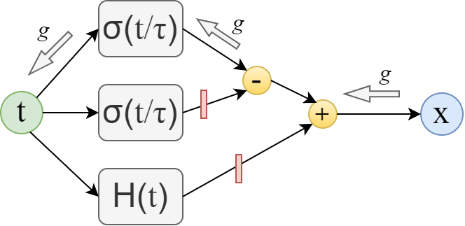
Figure 8: Computation graph for the deterministic hot sigmoid

We present here the program code for computing the stochastic sigmoid with temperature. Instead of the Heaviside function we will use rounding of the sigmoid output, which leads to the same result (and it is faster in the pytorch framework). The values of x_hard— are, while real, but nevertheless discrete values of $0$ or $1$. When calculating this quantity, there is a detachment from the graph (Then we add the difference between the numerically equal values of (the grouping by parentheses around the difference is important to avoid the loss of precision). Since one of the terms (In Figure 8, detachment from the graph is denoted by the red vertical bars. The forward computation runs left-to-right along the graph, and the gradient $g$ propagates right-to-left.

⬇

def hot_sigmoid(t, tau=1., s=1., hard=True, rand=True, eps=1e-8):

if rand:

r = torch.rand_like(t) # ~ U(0,1)

r = torch.log(eps + r / (1-r+eps)) # ~ L(0,1)

t = t + s * r # + L(0,s)

x_soft = torch.sigmoid(t/tau)

if not hard:

return x_soft

x_hard = x_soft.detach().round()

return x_hard + (x_soft - x_soft.detach())

If the version of the step-function. In the For generality, we will also combine the deterministic and stochastic functions into one (parameter

Appendix B CONstrained Gradient descent with Adaptation

Suppose that the change of parameters leads to escape into the forbidden region of the search space (a penalty is triggered): $w(\mathbf{x})>0$. Then the loss function (2) and its gradient would have the form:

$$L=-v+\frac{\gamma}{\nu}\,w^{\nu},\leavevmode\nobreak\ \leavevmode\nobreak\ \leavevmode\nobreak\ \leavevmode\nobreak\ \leavevmode\nobreak\ \leavevmode\nobreak\ \leavevmode\nobreak\ \nabla L=-\nabla v+\gamma\,w^{\nu-1}\,\nabla w.$$ (8)

We choose $\gamma$ so that $w(\mathbf{x})$ decreases in the next step of the gradient method:

$$w(\mathbf{x}-\lambda\,\nabla L)=(1-\mu)\,w(\mathbf{x}),$$ (9)

where $\mu\in[0...1]$ is a constant (another hyperparameter). The closer $\mu$ is to unity, the more strongly $w$ decreases. Assuming that the change in the parameters $\lambda\,\nabla L$ is small, let us expand the left part of the equality into a Taylor series: $w(\mathbf{x}-\lambda\,\nabla L)\approx w(\mathbf{x})-\lambda\,\nabla L\,\nabla w(\mathbf{x})$ and substitute $\nabla L$. This yields the following value for the factor at penalty:

$$\gamma=\frac{\nabla v\nabla w+\mu\,w}{w^{\nu-1}\,(\nabla w)^{2}},\leavevmode\nobreak\ \leavevmode\nobreak\ \leavevmode\nobreak\ \leavevmode\nobreak\ \leavevmode\nobreak\ \leavevmode\nobreak\ \gamma=\max(0,\,\gamma).$$ (10)

Trimming the value of $\gamma$ from below is necessary to ensure that the weight of the penalty is not negative when $\nabla v\nabla w<0$. The possible singularity in the denominator is eliminated, as usual, by adding a small $\text{eps}\sim 10^{-6}$.

In the method described in [21], it is required that along with the decrease of $w$, the target function $v$ increases. The corresponding AGA (Adaptive Gradient Ascent) algorithm is as follows:

$$\gamma=\left\{\begin{array}[]{llll}0&\nabla v\nabla w<0&(1)\\ (r_{1}+r_{2})/2&\nabla v\nabla w>0\leavevmode\nobreak\ \leavevmode\nobreak\ \&\leavevmode\nobreak\ \leavevmode\nobreak\ r_{1}<r_{2}&(2)\\ r_{3}&\text{otherwise}&(3)\end{array}\right.$$ (11)

where

$$r_{1}=\frac{\nabla v\nabla w}{w^{\nu-1}\,(\nabla w)^{2}},\leavevmode\nobreak\ \leavevmode\nobreak\ \leavevmode\nobreak\ \leavevmode\nobreak\ \leavevmode\nobreak\ r_{2}=\frac{(\nabla v)^{2}}{w^{\nu-1}\,\nabla v\nabla w},\leavevmode\nobreak\ \leavevmode\nobreak\ \leavevmode\nobreak\ \leavevmode\nobreak\ \leavevmode\nobreak\ r_{3}=\frac{\nabla v\nabla w+w/\lambda}{w^{\nu-1}\,(\nabla w)^{2}}.$$

In fact, when $\nabla v\nabla w>0$, it is almost always $r_{1}<r_{2}$, since this inequality is not satisfied only when the gradients of $\nabla v$ and $\nabla w$ are exactly parallel (or antiparallel). Therefore, the third condition is rarely satisfied.

Note that the original AGA method is quite sensitive to the learning rate $\lambda$. Figure 9 shows the trajectories of the gradient method from the same point at different $\lambda$. The blue circle outlines the region covering the allowed solutions. The color of the points corresponds to the three conditions of the AGA method in (11) and the zero index is given to the points inside the allowed region.

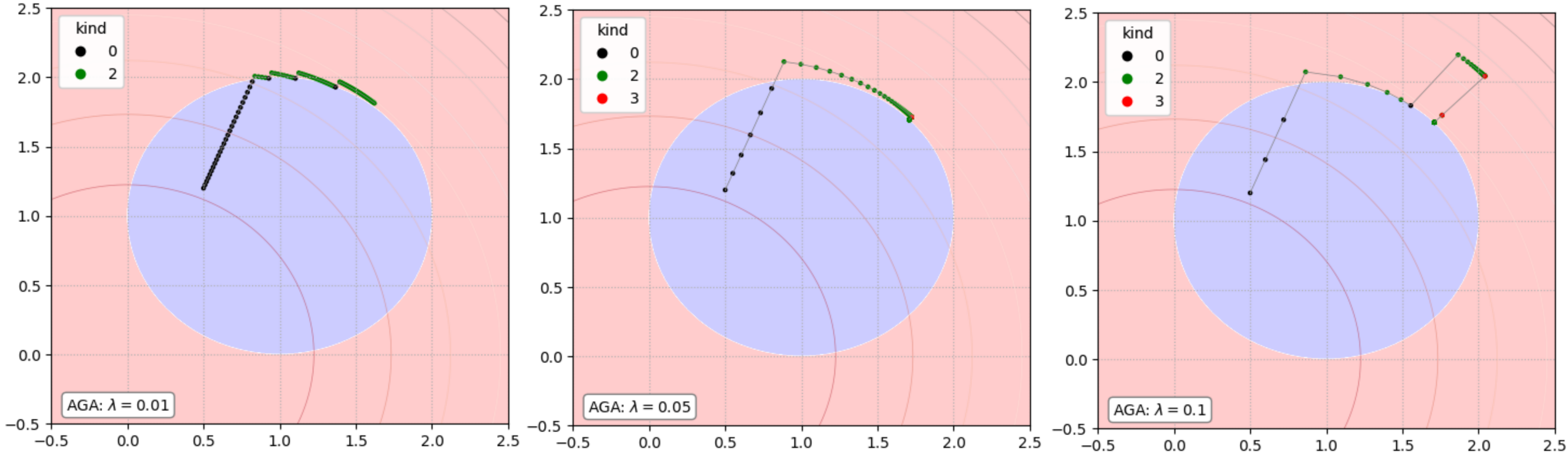
Figure 9: Search for the optimal solution by the AGA method for different $\lambda$. Throughout the following, the target function $v=x^{2}+y^{2}=\max$ and $\mathbf{x}=\{x,y\}$ are assumed to be continuous. The constraint function: $w=(x-1)^{2}+(y-1)^{2}-1\leq 0$

The CONGA method proposed in this paper is significantly less sensitive to the choice of learning rate (see Fig. 10).

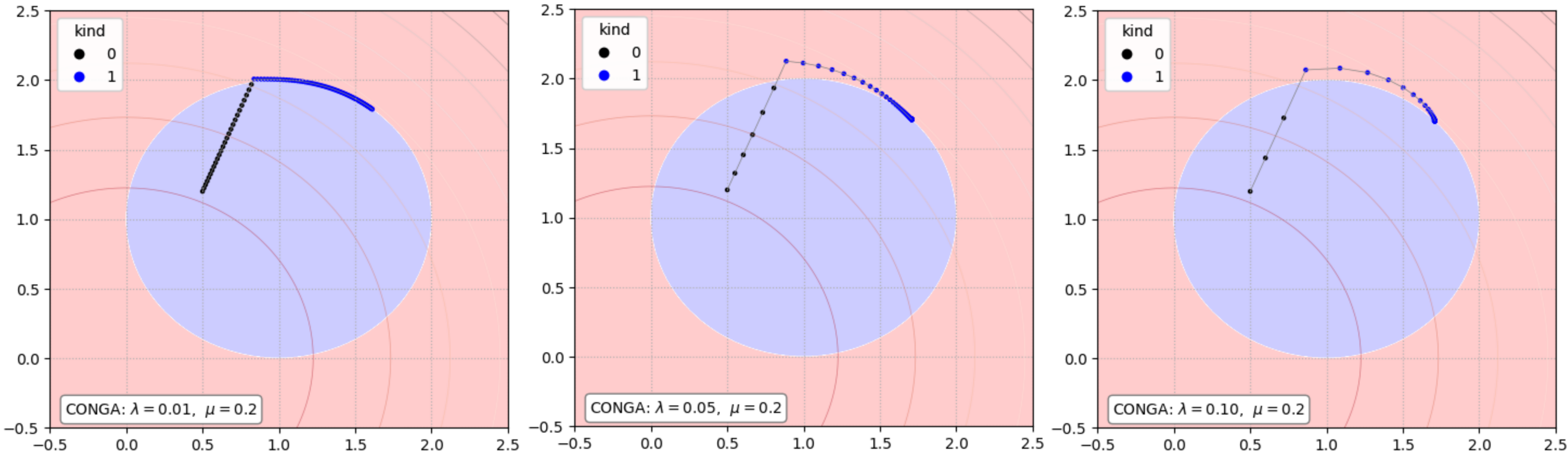
Figure 10: Search for the optimal solution by the CONGA method for different $\lambda$.

The second advantage of CONGA comes from the presence of a hyperparameter $\mu$, which regulates the desired ’attraction’ of the iterative procedure to the interior of the allowed region. Figure 11 shows a solution that starts in the forbidden region. The first graph corresponds to the AGA method, and the second and third to different values of the hyperparameter $\mu$ in the CONGA method.

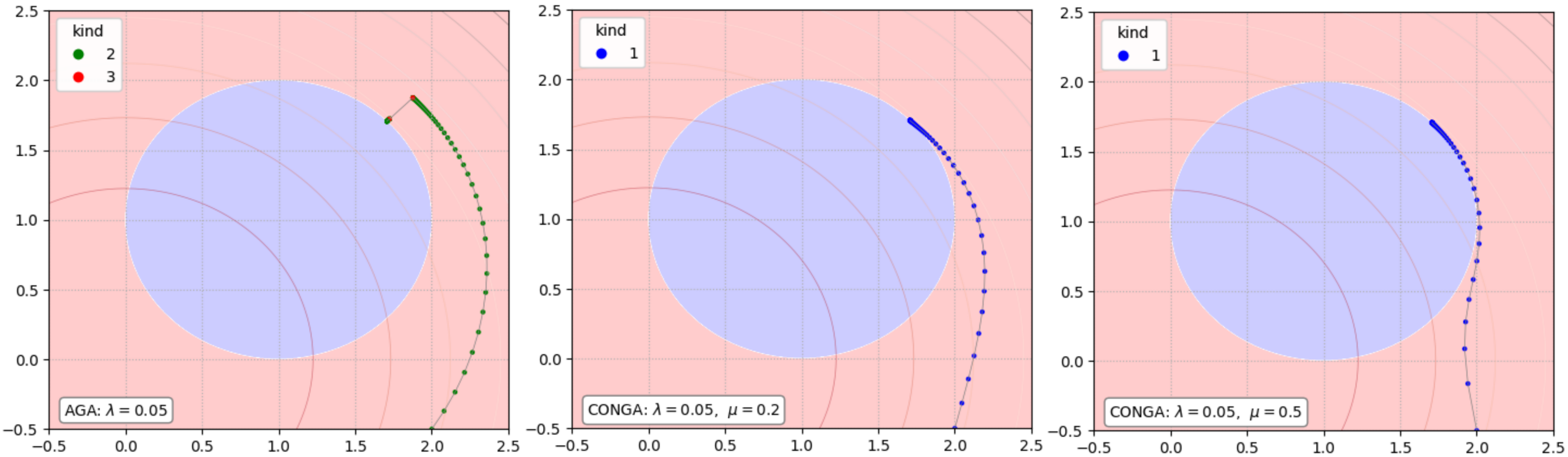
Figure 11: Search for the optimal solution starting from the forbidden region: AGA method compared to CONGA (for 2 different values of $\mu$). The closer $\mu$ is to $1$, the more strongly the solution is pushed to the boundary.

Another important feature of CONGA is the introduction of exponential smoothing for the gradient $\nabla v$ (with the parameter $\beta_{v}\in[0...1]$) and $\nabla w$ (with the parameter $\beta_{w}\in[0...1]$):

$$V_{k+1}=\beta_{v}\,V_{k}+(1-\beta_{v})\,\nabla v_{k},\leavevmode\nobreak\ \leavevmode\nobreak\ \leavevmode\nobreak\ \leavevmode\nobreak\ \leavevmode\nobreak\ \leavevmode\nobreak\ \leavevmode\nobreak\ \leavevmode\nobreak\ \leavevmode\nobreak\ \leavevmode\nobreak\ W_{k+1}=\beta_{w}\,W_{k}+(1-\beta_{w})\,\nabla w_{k}$$ (12)

The closer $\beta_{w}$ is to $1$, the deeper the iteration can penetrate into the forbidden region, while still eventually converging to the valid solution. This allows us to find an optimal solution even in situations where the constraint is not a convex function (Figure 12).

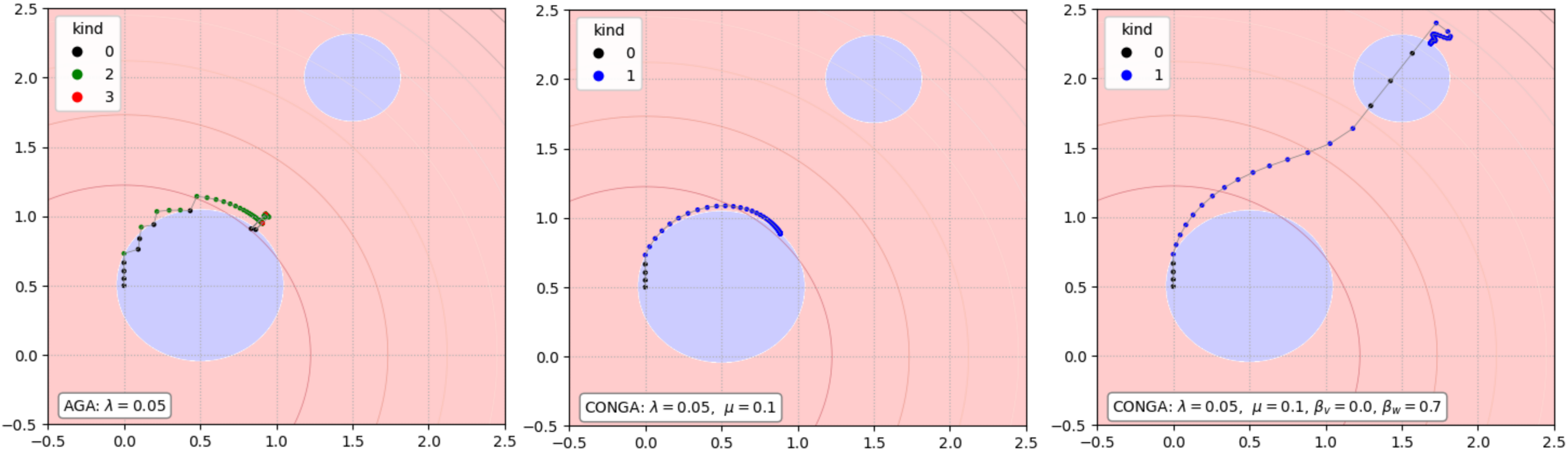
Figure 12: Search for an optimal solution for a non-convex constraint function by AGA, CONGA w/o EMA and CONGA with EMA methods.

Appendix C Summary of CONGA Method Application

We present here the comparison of our results to several other algorithms. To compare the results of the CONGA method proposed in this paper, the following algorithms for solving the 0–1 KP problem were used: Branch and Bound (BB), Genetic Algorithm (GA), Greedy Search Algorithm (GSA) and Simulated Annealing (SA). One recent review of these algorithms application to the dataset we use to test our method is given in [16]. Therefore, in this work, we solved the problems of the above dataset using the CONGA algorithm and compared it with benchmark results collected in [16].

The results of comparing the CONGA method with other algorithms by type of problem are presented in the Tables 3 (LD-UC datasets), 4 (HD-UC datasets), 5 (HD-WC datasets), and 6 (HD-SC datasets). The values of the hyperparameters used in our experiments are given in Table 2.

Table 2: Hyperparameters

[1.2pt] Hyper-parameter	Values	Description
[1pt] n_generations	2	number of generations
epochs	2000	maximum epochs per generation
n_agents	50	number of agents in generation
lr	1e-1	learning rate
nu	1.0	fraction of boundary part
mu1	0.2	minimum value of mu for initial distribution
mu2	0.8	maximum value of mu for initial distribution
beta_v	0.5	EMA beta for values gradient
beta_w	0.5	EMA beta for weights gradient
eps	1e-6	avoid zero div in gamma calc
tau1	30	initial temperature for hot sigmoid
tau_hot	30	hot temperature value at tau_warmap_epochs
tau2	0.01	final temperature value at tau_max_epochs
tau_warmap_epochs	1	epochs where temperature reaches tau_hot
tau_max_epochs	2000	epochs where temperature reaches tau2
[1.2pt]

Table 3: Results obtained on LD-UC datasets.

[2pt] Algorithm	Dataset	Items	Best Value	Optimal Value	Shortfall
[2pt] BB	f1_1-d_kp_10_269	10	280	295	15
GA	f1_1-d_kp_10_269	10	295	295	0
GSA	f1_1-d_kp_10_269	10	288	295	7
SA	f1_1-d_kp_10_269	10	294	295	1
CONGA	f1_1-d_kp_10_269	10	295	295	0
[1pt] BB	f2_1-d_kp_20_878	20	972	1024	52
GA	f2_1-d_kp_20_878	20	1024	1024	0
GSA	f2_1-d_kp_20_878	20	1024	1024	0
SA	f2_1-d_kp_20_878	20	972	1024	52
CONGA	f2_1-d_kp_20_878	20	1024	1024	0
[1pt] BB	f3_1-d_kp_4_20	4	24	35	11
GA	f3_1-d_kp_4_20	4	35	35	0
GSA	f3_1-d_kp_4_20	4	28	35	7
SA	f3_1-d_kp_4_20	4	35	35	0
CONGA	f3_1-d_kp_4_20	4	35	35	0
[1pt] BB	f4_1-d_kp_4_11	4	22	23	1
GA	f4_1-d_kp_4_11	4	23	23	0
GSA	f4_1-d_kp_4_11	4	19	23	4
SA	f4_1-d_kp_4_11	4	22	23	1
CONGA	f4_1-d_kp_4_11	4	23	23	0
[1pt] BB	f5_1-d_kp_15_375	15	469,16	481,07	11,91
GA	f5_1-d_kp_15_375	15	477	481,07	4,07
GSA	f5_1-d_kp_15_375	15	481,07	481,07	0
SA	f5_1-d_kp_15_375	15	481,07	481,07	0
CONGA	f5_1-d_kp_15_375	15	481,07	481,07	0
[1pt] BB	f6_1-d_kp_10_60	10	49	52	3
GA	f6_1-d_kp_10_60	10	52	52	0
GSA	f6_l-d_kp_10_60	10	43	52	9
SA	f6_l-d_kp_10_60	10	52	52	0
CONGA	f6_l-d_kp_10_60	10	52	52	0
[1pt] BB	f7_1-d_kp_7_50	7	96	107	11
GA	f7_1-d_kp_7_50	7	107	107	0
GSA	f7_l-d_kp_7_50	7	100	107	7
SA	f7_1-d_kp_7_50	7	102	107	5
CONGA	f7_1-d_kp_7_50	7	107	107	0
[2pt]

Table 4: Results obtained on HD-UC datasets.

[2pt] Algorithm	Dataset	Items	Best Value	Optimal Value	Shortfall
[2pt] SA	knapPI_1_100_1000_1	100	9147	9147	0
GA	knapPI_1_100_1000_1	100	9147	9147	0
GSA	knapPI_1_100_1000_1	100	2983	9147	6164
BB	knapPI_1_100_1000_1	100	8026	9147	1121
CONGA	knapPI_1_100_1000_1	100	9147	9147	0
[1pt] SA	knapPI 1 200_1000_1	200	10163	11238	1075
GA	knapPI 1 200_1000_1	200	102340	11238	-91102
GSA	knapPI 1 200_1000_1	200	4544	11238	6694
BB	knapPI_1_200_1000_1	200	10436	11238	802
CONGA	knapPI_1_200_1000_1	200	11238	11238	0
[1pt] SA	knapPI_1_500_1000_1	500	21390	28857	7467
GA	knapPI_1_500_1000_1	500	102340	28857	-73483
GSA	knapPI_1_500_1000_1	500	9865	28857	18992
BB	knapPI_1_500_1000_1	500	28043	28857	814
CONGA	knapPI_1_500_1000_1	500	28857	28857	0
[1pt] SA	knapPI_1_1000_1000_1	1000	36719	54503	17784
GA	knapPI_1_1000_1000_1	1000	130	54503	54373
GSA	knapPI_1_1000_1000_1	1000	14927	54503	39576
BB	knapPI_1_1000_1000_1	1000	53397	54503	1106
CONGA	knapPI_1_1000_1000_1	1000	54503	54503	0
[1pt] SA	knapPI_1_2000_1000_1	2000	65793	110625	44832
GA	knapPI_1_2000_1000_1	2000	102340	110625	8285
GSA	knapPI_1_2000_1000_1	2000	25579	110625	85046
BB	knapPI_1_2000_1000_1	2000	109679	110625	946
CONGA	knapPI_1_2000_1000_1	2000	110625	110625	0
[1pt] SA	knapPI_1_5000_1000_1	5000	150731	276457	125726
GA	knapPI_1_5000_1000_1	5000	102340	276457	174117
GSA	knapPI_1_5000_1000_1	5000	49306	276457	227151
BB	knapPI_1_5000_1000_1	5000	275720	276457	737
CONGA	knapPI_1_5000_1000_1	5000	276457	276457	0
[1pt] SA	knapPI_1_10000_1000_1	10000	563647	563647	0
GA	knapPI_1_10000_1000_1	10000	562556	563647	1091
GSA	knapPI_1_10000_1000_1	10000	292255	563647	271392
BB	knapPI_1_10000_1000_1	10000	130	563647	563517
CONGA	knapPI_1_10000_1000_1	10000	563647	563647	0
[2pt]

Table 5: Results obtained on HD-WC datasets.

[2pt] Algorithm	Dataset	Items	Best Value	Optimal Value	Shortfall
[2pt] SA	knapPI_2_100_1000_1	100	1486	1514	28
GA	knapPI_2_100_1000_1	100	1158	1514	356
GSA	knapPI_2_100_1000_1	100	1041	1514	473
BB	knapPI_2_100_1000_1	100	1440	1514	74
CONGA	knapPI_2_100_1000_1	100	1514	1514	0
[1pt] SA	knapPI_2_1000_1000_1	1000	6831	9052	2221
GA	knapPI_2_1000_1000_1	1000	7912	9052	1140
GSA	knapPI_2_1000_1000_1	1000	5675	9052	3377
BB	knapPI_2_1000_1000_1	1000	9006	9052	46
CONGA	knapPI_2_1000_1000_1	1000	9052	9052	0
[1pt] SA	knapPI_2_10000_1000_1	10000	57852	90204	32352
GA	knapPI_2_10000_1000_1	10000	79615	90204	10589
GSA	knapPI_2_10000_1000_1	10000	54447	90204	35757
BB	knapPI_2_10000_1000_1	10000	90073	90204	131
CONGA	knapPI_2_10000_1000_1	10000	90204	90204	0
[1pt] SA	knapPI_2_200_1000_1	200	1537	1634	97
GA	knapPI_2_200_1000_1	200	1306	1634	328
GSA	knapPI_2_200_1000_1	200	1073	1634	561
BB	knapPI_2_200_1000_1	200	1603	1634	31
CONGA	knapPI_2_200_1000_1	200	1634	1634	0
[1pt] SA	knapPI_2_2000_1000_1	2000	12780	18051	5271
GA	knapPI_2_2000_1000_1	2000	15887	18051	2164
GSA	knapPI_2_2000_1000_1	2000	11064	18051	6987
BB	knapPI_2_2000_1000_1	2000	17794	18051	257
CONGA	knapPI_2_2000_1000_1	2000	18051	18051	0
[1pt] SA	knapPI_2_500_1000_1	500	3744	4566	822
GA	knapPI_2_500_1000_1	500	3701	4566	865
GSA	knapPI_2_500_1000_1	500	2951	4566	1615
BB	knapPI_2_500_1000_1	500	4484	4566	82
CONGA	knapPI_2_500_1000_1	500	4566	4566	0
[1pt] SA	knapPI_2_5000_1000_1	5000	29220	44356	15136
GA	knapPI_2_5000_1000_1	5000	37746	44356	6610
GSA	knapPI_2_5000_1000_1	5000	27387	44356	16969
BB	knapPI_2_5000_1000_1	5000	44198	44356	158
CONGA	knapPI_2_5000_1000_1	5000	44356	44356	0
[2pt]

Table 6: Results obtained on HD-SC datasets.

[2pt] Algorithm	Dataset	Items	Best Value	Optimal Value	Shortfall
[2pt] SA	knapPI_3_100_1000_1	100	2296	2397	101
GA	knapPI_3_100_1000_1	100	2091	2397	306
GSA	knapPI_3_100_1000_1	100	1095	2397	1302
BB	knapPI_3_100_1000_1	100	2268	2397	129
CONGA	knapPI_3_100_1000_1	100	2397	2397	0
[1pt] SA	knapPI_3_1000_1000_1	1000	11789	14390	2601
GA	knapPI_3_1000_1000_1	1000	13090	14390	1300
GSA	knapPI_3_1000_1000_1	1000	5589	14390	8801
BB	knapPI_3_1000_1000_1	1000	14271	14390	119
CONGA	knapPI_3_1000_1000_1	1000	14390	14390	0
[1pt] SA	knapPI_3_10000_1000_1	10000	106114	146919	40805
GA	knapPI_3_10000_1000_1	10000	124719	146919	22200
GSA	knapPI_3_10000_1000_1	10000	54518	146919	92401
BB	knapPI_3_10000_1000_1	10000	146787	146919	132
CONGA	knapPI_3_10000_1000_1	10000	146919	146919	0
[1pt] SA	knapPI_3_200_1000_1	200	2594	2697	103
GA	knapPI_3_200_1000_1	200	25319	2697	-22622
GSA	knapPI_3_200_1000_1	200	1095	2697	1602
BB	knapPI_3_200_1000_1	200	2542	2697	155
CONGA	knapPI_3_200_1000_1	200	2697	2697	0
[1pt] SA	knapPI_3_2000_1000_1	2000	22482	28919	6437
GA	knapPI_3_2000_1000_1	2000	25319	28919	3600
GSA	knapPI_3_2000_1000_1	2000	10818	28919	18101
BB	knapPI_3_2000_1000_1	2000	28726	28919	193
CONGA	knapPI_3_2000_1000_1	2000	28919	28919	0
[1pt] SA	knapPI_3_500_1000_1	500	6103	7117	1014
GA	knapPI_3_500_1000_1	500	6517	7117	600
GSA	knapPI_3_500_1000_1	500	2916	7117	4201
BB	knapPI_3_500_1000_1	500	6995	7117	122
CONGA	knapPI_3_500_1000_1	500	7117	7117	0
[1pt] SA	knapPI_3_5000_1000_1	5000	53672	72505	18833
GA	knapPI_3_5000_1000_1	5000	61904	72505	10601
GSA	knapPI_3_5000_1000_1	5000	27304	72505	45201
BB	knapPI_3_5000_1000_1	5000	72345	72505	160
CONGA	knapPI_3_5000_1000_1	500	72505	72505	0
[2pt]

References

- [1] Junyoung Chung, Sungjin Ahn and Yoshua Bengio “Hierarchical multiscale recurrent neural networks”, 2016 arXiv:1609.01704
- [2] Chris J. Maddison, Andriy Mnih and Yee Whye Teh “The Concrete Distribution: A Continuous Relaxation of Discrete Random Variables”, 2017 arXiv:1611.00712 [cs.LG]
- [3] Eric Jang, Shixiang Gu and Ben Poole “Categorical Reparameterization with Gumbel-Softmax”, 2017 arXiv:1611.01144 [stat.ML]
- [4] Yoshua Bengio, Nicholas Léonard and Aaron Courville “Estimating or Propagating Gradients Through Stochastic Neurons for Conditional Computation” arXiv, 2013 DOI: 10.48550/ARXIV.1308.3432
- [5] Iris AM Huijben, Wouter Kool, Max B Paulus and Ruud JG Van Sloun “A review of the gumbel-max trick and its extensions for discrete stochasticity in machine learning” In IEEE Transactions on Pattern Analysis and Machine Intelligence 45.2 IEEE, 2022, pp. 1353–1371
- [6] Aaron Van Den Oord and Oriol Vinyals “Neural discrete representation learning” In Advances in neural information processing systems 30, 2017
- [7] Aditya Ramesh et al. “Zero-shot text-to-image generation” In International Conference on Machine Learning, 2021, pp. 8821–8831 PMLR
- [8] Hangbo Bao, Li Dong, Songhao Piao and Furu Wei “Beit: Bert pre-training of image transformers”, 2021 arXiv:2106.08254
- [9] Nicola De Cao and Thomas Kipf “MolGAN: An implicit generative model for small molecular graphs”, 2022 arXiv:1805.11973 [stat.ML]
- [10] Edward Choi et al. “Generating Multi-label Discrete Patient Records using Generative Adversarial Networks” arXiv, 2017 DOI: 10.48550/ARXIV.1703.06490
- [11] Gonzalo Mena, David Belanger, Scott Linderman and Jasper Snoek “Learning latent permutations with gumbel-sinkhorn networks”, 2018 arXiv:1802.08665
- [12] Yi Tay et al. “Sparse Sinkhorn Attention” arXiv, 2020 DOI: 10.48550/ARXIV.2002.11296
- [13] Hans Kellerer, Ulrich Pferschy and David Pisinger “Knapsack Problems” Springer Berlin Heidelberg, 2004 DOI: 10.1007/978-3-540-24777-7
- [14] David Pisinger “Where are the hard knapsack problems?” In Computers & Operations Research 32.9 Elsevier, 2005, pp. 2271–2284
- [15] Jorik Jooken, Pieter Leyman and Patrick De Causmaecker “Features for the 0-1 knapsack problem based on inclusionwise maximal solutions” In European Journal of Operational Research 311.1, 2023, pp. 36–55 DOI: https://doi.org/10.1016/j.ejor.2023.04.023
- [16] Absalom E. Ezugwu et al. “A Comparative Study of Meta-Heuristic Optimization Algorithms for 0 – 1 Knapsack Problem: Some Initial Results” In IEEE Access 7, 2019, pp. 43979–44001 DOI: 10.1109/ACCESS.2019.2908489
- [17] Soukaina Laabadi, Mohamed Naimi, Hassan El Amri and Boujemâa Achchab “The 0/1 Multidimensional Knapsack Problem and Its Variants: A Survey of Practical Models and Heuristic Approaches” In American Journal of Operations Research 08.05 Scientific Research Publishing, Inc., 2018, pp. 395–439 DOI: 10.4236/ajor.2018.85023
- [18] Jakob Puchinger, Günther R. Raidl and Ulrich Pferschy “The Multidimensional Knapsack Problem: Structure and Algorithms” In INFORMS Journal on Computing 22.2 Institute for Operations Researchthe Management Sciences (INFORMS), 2010, pp. 250–265 DOI: 10.1287/ijoc.1090.0344
- [19] Oriol Vinyals, Meire Fortunato and Navdeep Jaitly “Pointer Networks” arXiv, 2015 DOI: 10.48550/ARXIV.1506.03134
- [20] Shenshen Gu and Tao Hao “A pointer network based deep learning algorithm for 0–1 Knapsack Problem” In 2018 Tenth International Conference on Advanced Computational Intelligence (ICACI), 2018, pp. 473–477 DOI: 10.1109/ICACI.2018.8377505
- [21] Duanshun Li et al. “A novel method to solve neural knapsack problems” In International Conference on Machine Learning 139, Proceedings of Machine Learning Research PMLR, 2021, pp. 6414–6424 PMLR URL: https://proceedings.mlr.press/v139/li21m.html
- [22] David Pisinger “Instances of 0/1 Knapsack Problem”, 2018 URL: http://artemisa.unicauca.edu.co/~johnyortega/instances_01_KP/