Surrogate Neural Networks Local Stability for Aircraft Predictive Maintenance

Abstract

Surrogate Neural Networks (NN) now routinely serve as substitutes for computationally demanding simulations (e.g.,  finite element). They enable faster analyses in industrial applications e.g., manufacturing processes, performance assessment. The verification of surrogate models is a critical step to assess their robustness under different scenarios. We explore the combination of empirical and formal methods in one NN verification pipeline. We showcase its efficiency on an industrial use case of aircraft predictive maintenance. We assess the local stability of surrogate NN designed to predict the stress sustained by an aircraft part from external loads. Our contribution lies in the complete verification of the surrogate models that possess a high-dimensional input and output space, thus accommodating multi-objective constraints. We also demonstrate the pipeline effectiveness in substantially decreasing the runtime needed to assess the targeted property.

1 Introduction

There have been significant advances in the development of verification methods assessing the resilience of NN against perturbations, often represented by $l_{p}$ norm balls. These approaches have proven promising in providing NN robustness assessment, and may allow one day to meet the emerging certification requirements for NN use in critical systems such as aviation. Notable references include guidelines from certification and aviation standardization entities advocating for the use of formal methods as a mean of compliance to ensure model robustness. A concrete example of this progress is the Formal Methods use for Learning Assurance (ForMuLA (2023)) report, published from the partnership between European Aviation Safety Agency (EASA) and Collins Aerospace. It relies on an industrial use case (prediction of the remaining useful life of aeronautical components) to illustrate how formal methods can be used to assess the safety of ML based systems. Although the predominant focus of formal method applications has been on classification tasks, there has been comparatively less emphasis on regression tasks, especially those tailored for industrial applications. It is crucial to highlight however the relevance of pushing these methods for regression in regard to the increasing use of NN surrogate models in the aviation industry, e.g., substituting computationally-demanding finite elements simulations.

In this paper, we are investigating the robustness of a NN surrogate model in the context of predictive aircraft maintenance. By taking into account the unique specificities of our use case (e.g., multiple inputs and outputs, regression task etc.) and the domain constraints of predictive maintenance, our case-study offers a unique opportunity to explore a pragmatic process of robustness verification for surrogate models developed for a concrete civil aviation application.

2 Use case: Aircraft Loads-to-Stress Prediction

2.1 Description

In aeronautics, numerical simulations are used to model system physical phenomena (e.g., finite element) but, due to computational cost, querying them in real-time or embedding them in larger processes is unpractical. Their application therefore remains limited to the design phase and particular cases. Their use could however greatly improve productivity e.g. in predictive maintenance. Currently, structural maintenance programs are based on conservative design assumptions aiming to cover a variety of aircraft usage in the fleet. Therefore, there is a benefit in introducing optimised maintenance, tailored to individual aircraft to reduce maintenance cost as well as ensure safety of operations is maintained at the highest level. Custom solutions, however, require the analysis of large amount of data (e.g., flight history), not practical with the current solutions.

NN are a game changer. Studies have shown the value of NN-based surrogates to approximate numerical simulators (e.g., Sudakov et al. (2019)). Their use, however, requires the maturation of new processes for a safe use. In this analysis, we investigate an example of NN surrogate model: the prediction of the stress level in part of an aircraft structure from sustained external loads. The accurate evaluation of the stresses is a key enabler for maintenance optimization.

We consider a number of NNs composed of $2$ hidden layers ($h$) with 165 neurons ($r$), followed by ReLU activation functions. They predict $81$ normalised stress outputs ($k$) from $216$ normalised loads input variables ($n$). These NNs are research prototypes. They are trained with various epochs (from $2$ to $10000$). These feed-forward NNs are functions we denote as $f:\mathbb{R}^{n}\mapsto\mathbb{R}^{k}$. Let $x$ be an input vector of dimension $n$, $W$ the weights and $b$ the biases of the network. A function $f$ is the composition of linear functions denoted $l_{i}:x\mapsto W_{i}\cdot x+b_{i}$ and followed by element-wise non linear activation functions denoted $\sigma$. We only consider ReLU activations, such that $\sigma:x\in\mathbb{R}^{k}\mapsto[max(x_{j},0)]_{j=1}^{r}$. Therefore, we can express the NNs as the following: $f(x):x\mapsto W_{i}\cdot h_{i}(x)+b_{i}$, with $h_{i\geq 1}:x\mapsto\sigma\Big{(}l_{i-1}\big{(}h_{i-1}(x)\big{)}\Big{)}$ and $h_{0}:x\mapsto x$.

2.2 Property specification to be ensured: Local stability

Local stability ensures that NN predictions are consistent in the vicinity of test data where the model is not explicitly trained. In sensitive domains such as aeronautics, NN local stability is a critical requirement as it reflects physical characteristics: the prediction of stress from loads inherently possesses a local stability well known by aeronautical engineers. Requirements are enunciated in property 1 and are essentially split in two zones. We will refer to this property as the ‘bow tie’ owing to its distinctive shape. The belonging to a given zone for a data point $x$ to be verified is defined by the output value $f(x)$.

Property 1

The ‘Bow tie’

Consider a NN $f$, an input sample $x\in\mathbb{R}^{n}$, a local perturbation $p$ such that $x^{\prime}\in\big{[}x-p_{inp}.|x|,x+p_{inp}.|x|\big{]}$. The local stability is ensured if:

$$\underline{\delta}\leq f(x^{\prime})-f(x)\leq\overline{\delta}$$

$$[\underline{\delta},\overline{\delta}]=\begin{cases}[-c_{T},c_{T}]&\text{if }|f(x)|\leq T\\ &\text{(`Knot')}\\ [-p_{out},p_{out}].|f(x)|&\text{else}\\ &\text{(`Wings')}\\ \end{cases}$$

Stability is guaranteed if property 1 is proven for all $81$ outputs. Taking into account domain expertise related to the use case and the required stability properties, we choose $T=10$, $c_{T}=1$ and $p_{inp}=p_{out}=0.05$.

3 Local stability assessment via methods combination

Before the advent of NN verification methods, stability was assessed via a random sampling of its ‘neighborhood’, a technique both partial and heavy when the number of outputs is high. There was therefore a crucial need for more formal and time-efficient means to assess stability. Formal verification involves both complete and incomplete methods. Complete methods have the capability to provide definite guarantees whereas incomplete methods are not always able to determine whether a property is unsatisfied. In a complementary manner, empirical techniques such as adversarial attacks exploit vulnerabilities by adding perturbations to inputs and make a model produce incorrect outputs. Hence, exploring a combination of techniques is the next obvious step. We converge towards the sequential use of the following techniques (summarized in Fig. 1):

A- Empirical approaches. To minimize the need for time-consuming formal approaches, the first verification step relies on generating attacks. If one is found (on even only one of the outputs), its stability is proven wrong. Attacks intent to ‘push’ predictions beyond the bow tie while staying within the allowed noise and are performed for each output $j$ separately i.e., we intend to increase $|f_{j}(x)-f_{j}(x^{\prime})|$, independently of the effect on other indexes. The attack implementation is designed to create either a positive or a negative property violation (beyond $\overline{\delta}$ or $\underline{\delta}$). We conduct experiments with several classical attacks using the cleverhans library e.g., PGD: Projected Gradient Descent (Madry et al. (2017)).

B- Incomplete formal methods. We make use of the linear relaxation-based verification bound method CROWN (Zhang et al. (2018)) implemented within the decomon library (Ducoffe (2021)). The use of incomplete methods is to converge towards a stability guarantee for most of the test data and leverage their less computationally-demanding nature compared to complete techniques.

C- Complete formal methods. To evaluate test points whose stability is neither refuted nor guaranteed by the previous methods, we use an in-house Mixed-Integer Linear Program (MILP)-based verifier. Encoding of the network into variables and constraints is done similarly to the Venus library (Botoeva et al. (2020)). Symbolic interval propagation is used to provide bounds for neuron values. Details on the implementation are provided in Appendix B.

4 Results

The assessment of local stability (§2.1) is performed on $1000$ test points. All experiments are conducted on a machine equipped with an Apple M2 Pro processor and $32$ GB of memory. The MILP based solver is running with Gurobi 10.0 version. This section discusses the key findings and outcomes of our study.

Fig 1 illustrates the technique sequence used to assess NN stability and how the NN verification is performed on the ‘2-epoch’ model. It shows subsets of the $1000$ test points progressing through the different stages (ABC), thus indicating whether their stability is verified (✓), violated (X), or non-guaranteed (?).

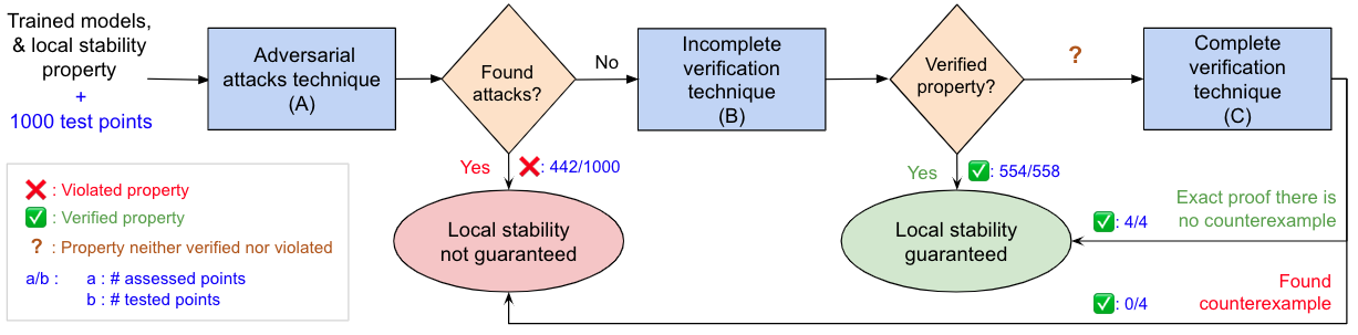
Figure 1: Overview of our verification pipeline for NN stability assessment.

		(1)	(2)	(3)	(4)	(5)	(6)
		A	B	C	A+C	B+C	Pipeline A+B+C
model 2	#Tested	1000	1000	1000	1000/558	1000/446	1000/558/4
	#Verified	-	554	558	558	558	-/554/4 = 558
	#Violated	442	-	442	442	442	442/-/0 = 442
	Runtime	10.7	3.3	267	19.8	267	10.7/1.96/3.91 = 16.6
model 500	#Tested	1000	1000	1000	1000/552	1000/471	1000/552/23
	#Verified	-	529	552	552	552	-/529/23 = 552
	#Violated	448	-	448	448	448	448/-/0 = 448
	Runtime	11.5	3.4	1091	580	827	11.5/1.9/307 = 320

Table 1: Stability assessment of $2$ and $500$-epoch models. Columns 1-3 correspond to experiments with only A- adversarial, B- incomplete and C- complete techniques. Columns 4-6 show combinations of these. ‘#Tested’ refers to the number of test data entering a verification brick. ‘#Verified’ refers to points whose property is guaranteed and ‘#Violated’ to the fact that a counterexample is found. ‘-’ means the technique can not prove that property status. ‘0’ shows it can but did not. Runtimes are provided in seconds.

Table 1 shows the stability assessments performed on two models using our verification pipeline. PGD attacks are generated using $20$ iterations of step size $\epsilon=0.01$. The MILP verifier was run with a timeout $t=300$s per point. We note that adversarial attacks can only provide ‘Violated’ status, but cannot guarantee the property. CROWN, on the opposite, can only prove points are ‘Verified’ i.e., guarantee stability but not its lack of. Only complete techniques can unequivocally prove that a point stability is either guaranteed or not.

Our core results are:

• A significant verification time gain: A factor of $3-16$% in runtime is obtained by combining verification methods instead of solely using complete approaches. The use of MILP-only verification takes $267$s ($1091$s) for the $2$- ($500$-)epoch model. In contrast, the cumulative time for the full pipeline is only $16.6$s ($320$s). Similarly, it has a faster runtime than a portion of it (e.g., Bricks A+C) which proves the effectiveness of combining techniques, thereby reducing the call to time-demanding exact computations. Details on the origin of the equal runtime between technique C-only and B+C for the 2-epoch model is explained in Appendix B. Pragmatically, we acknowledge that the more a model is robust, the more challenging it is to generate attacks and that runtime will increase with the use of formal techniques.

• Insights into our models: (i) Depending on the considered model and attack type, up to $45$% of the test data could be corrupted. Fig. 2 (in Appendix A) shows an example of these attack generations for our 50-epoch model. Some output indexes are found to be more vulnerable than others, a result that will be carefully considered for our on-going model optimisation. (ii) We find that the increase of training epochs does not make models less vulnerable to attacks (see Fig. 2 and Table 1). We suspect model overfitting may play a role in the decrease of model stability. It is also worth noting that the number of epochs negatively affects the performance of incomplete methods, leading to a longer verification time. (iii) We also show that attacks are preferentially found for $|f(x)|>10$. The requirement in the ‘knot’ stress regime is conservative enough that the property is almost never infringed.

5 Conclusions

This analysis presents the implementation and testing of a sound multi-technique verification pipeline for the a posteriori assessment of the local stability property of surrogate NN. By combining the strengths and mitigating the limitations of a number of techniques including adversarial attacks and complete and incomplete formal verification methods, we have not only manage to successfully perform a complete NN robustness assessment of our NN but also optimise the runtime of our experiments. Furthermore, our tests have also shade light on our model vulnerabilities as well as the potential consequence of design of our local stability property itself. This case-study only begins to explore what such verification pipeline could offer and further tuning of the techniques could lead to an even more time-efficient verification (see Appendix C). Beyond a posteriori assessment, we are now exploring the feasibility of strengthening our models by including empirical and formal components into our model design phase.

Appendix

A Example of adversarial attacks

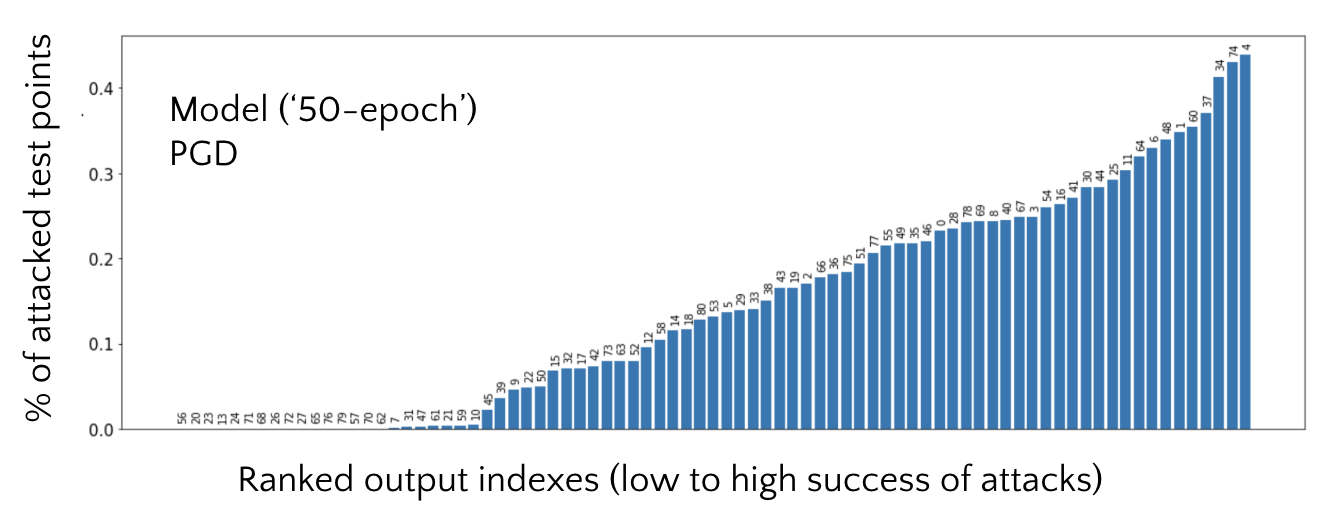
Figure 2: Percentage of successful PGD attacks for a given targeted output index (from $0$ to $80$; ranked with increasing success). Results are shown for the 50-epoch model. Attacks are generated for $1000$ test points. Each output index was attacked twice per test point (towards a positive or negative violation) resulting in a total of $2000$ attack attempts.

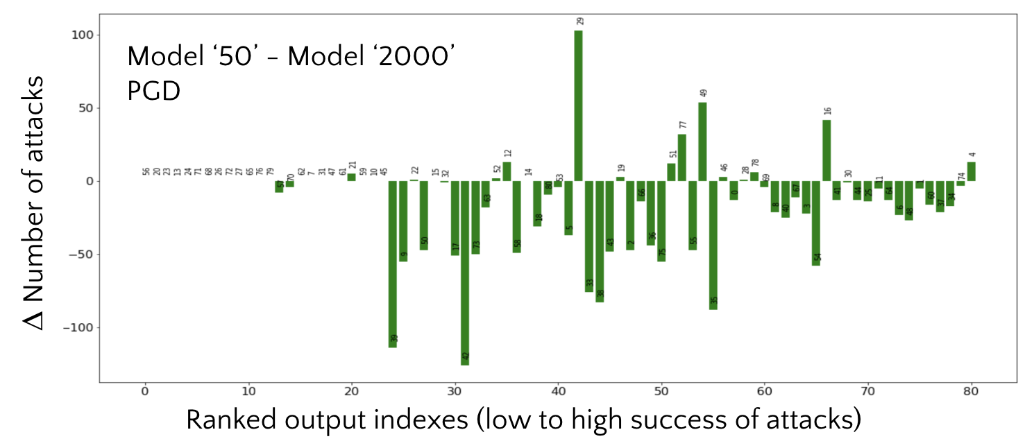
Figure 3: Difference of number of attacks (out of $2000$ attempts; see Fig.2) between the $50$-epoch and $2000$-epoch models. The $2000$-epoch model is clearly shown to be more vulnerable to attacks.

B Complete verification technique using MILP

B.1 Bound computation

A subtlety of the complete method used in the present analysis is that it uses bound propagation (Wang et al. [2018]) in order to provide lower and upper values to all neurons in the network. When the bound propagation is already able to reach a definite conclusion on the property, there is no call to the MILP solver (see Fig. 4).

Let’s now explain why the computation time of method A+C (Column 4, Table 1) is competitive with respect to the full pipeline on the 2-epoch model. On this lightly trained model, the first step of bound propagation estimation already concludes on the robustness of input points, without the need for further MILP computations, for all except $4$ test points (similar to the full pipeline A+B+C). On the contrary, when using method B+C (Column 5), most of the points entering the complete method are not robust and the MILP solver has to be run to find counter-example to the property.

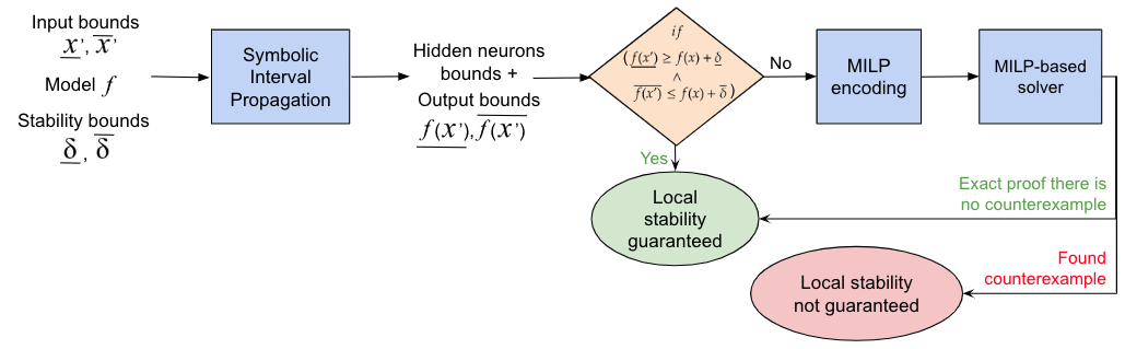
Figure 4: Sub-pipeline included in the MILP-based approach

B.2 MILP encoding of the neural network

The MILP encoding makes use of bounds computed by symbolic interval propagation. For each layer $i$ and neuron $j$ in the layer $i$, two continuous variables are created : $y_{i,j,-},y_{i,j,+}$ which corresponds to pre-activation and post-activation values of the neurons. Bounds of these variables are known thanks to the bound propagation function. Layer $i=0$ corresponds to input values.

The MILP is encoded as follow:

1. $\forall i\in[1,n_{layers}],j\in[0,n_{i}],y_{i,j,-}=W_{i}[j,:]*y_{i-1,:,+}+b_{i,j}$, where $W_{i}$ and $b_{i}$ are respectively the model weights and bias of layer $i$

2. $\forall i\in[1,n_{layers}]$, if layer $i$ is activated by a ReLu, $y_{i,j,+}=max(y_{i,j,-},0)$ else $y_{i,j,+}=y_{i,j-}$

The $max$ constraint is native into the Gurobi library and can be chosen instead of the classically used Big-M constraint (e.g., in Botoeva et al. [2020]).

B.3 Property encoding

Given $x,f(x),\underline{\delta},\overline{\delta}$ defined in property 1, we encode the negation of the property as follows:

1. Let $\forall j\in[1,81],indic_{-,j},indic_{+,j}$ be binary variables.

2. $\forall j,indic_{-,j}\rightarrow y_{n_{layers},j,+}\leq f(x)_{j}+\underline{\delta}$

3. $\forall j,indic_{+,j}\rightarrow y_{n_{layers},j,+}\geq f(x)_{j}+\overline{\delta}$

4. $\sum_{j}{(indic_{+,j}+indic_{-,j})}\geq 1$

Each indicator variable will encode the fact that for one output index, the perturbed NN prediction goes out of the bow-tie property. The last constraint thus encodes that the solver has to find a counter-example violating the property. If the MILP solver finds a solution, we conclude that the property is violated. On the contrary, if the solver proves the infeasibility of the model, we conclude that the property is verified.

C Foreseen optimisation of the verification pipeline

This case-study only begins to explore what such a verification pipeline could offer, and further tuning of the techniques could lead to an even more time-efficient verification.

For example, adversarial attacks are performed by order of output indexes while we find that some were more easily attackable than others. One could benefit from this knowledge to optimise the attack search on subsequent models.

We also experiment with hyperparameters tuning e.g., we test different numbers of iterations for a PDG attack and attempt to find a good compromise between the number of test points we successfully attack (in order not to have to use complete verification techniques further down the pipeline) and the total computing time of the adversarial attack stage (usually run on the larger test subsample). But further optimisation work could be done in that respect.

As far as the implementation of the MILP solver is concerned (see Appendix B), we are currently using symbolic interval propagation in order to provide starting bounds and restrict the input domain to be verified. For more complex NN however, interval arithmetic could provide excessively conservative bounds that may slow the verification. We are currently looking into using bounds derived from the inexact verification stage in order to feed them as initial bounds.

References

- Botoeva et al. [2020] E. Botoeva, P. Kouvaros, J. Kronqvist, A. Lomuscio, and R. Misener. Efficient verification of relu-based neural networks via dependency analysis. Proceedings of the AAAI Conference on Artificial Intelligence, 34:3291–3299, Apr. 2020.
- Ducoffe [2021] M. Ducoffe. Decomon: Automatic certified perturbation analysis of neural networks, 2021. URL https://github.com/airbus/decomon.
- ForMuLA [2023] ForMuLA. Formal methods use for learning assurance. Technical report, 2023.
- Madry et al. [2017] A. Madry, A. Makelov, L. Schmidt, D. Tsipras, and A. Vladu. Towards dl models resistant to adversarial attacks. arXiv preprint arXiv:1706.06083, 2017.
- O’Higgins et al. [2020] E. O’Higgins, K. Graham, D. Daverschot, and J. Baris. Machine Learning Application on Aircraft Fatigue Stress Predictions, pages 1031–1042. 01 2020. ISBN 978-3-030-21502-6. doi: 10.1007/978-3-030-21503-3˙81.
- Sudakov et al. [2019] O. Sudakov, D. Koroteev, B. Belozerov, and E. Burnaev. Artificial nn surrogate modeling of oil reservoir: a case study. In Advances in NN–ISNN 2019: 16th International Symposium on NN, ISNN 2019, Moscow, Russia, July 10–12, 2019, Proceedings, Part II 16, pages 232–241. Springer, 2019.
- Wang et al. [2018] S. Wang, K. Pei, J. Whitehouse, J. Yang, and S. Jana. Formal security analysis of neural networks using symbolic intervals. CoRR, 2018.
- Zhang et al. [2018] H. Zhang, T.-W. Weng, P.-Y. Chen, C.-J. Hsieh, and L. Daniel. Efficient neural network robustness certification with general activation functions. Advances in neural information processing systems, 31, 2018.