Supersymmetry in Quantum Mechanics by Generalized Uncertainty Principle

Abstract

In this paper, we study supersymmetry in quantum mechanics using the generalized uncertainty principle (GUP), or in other words, generalized supersymmetry in quantum mechanics. We construct supersymmetry in the generalized form of the momentum operator, which is derived from GUP. By generalizing the creation and annihilation operators, we can transform the supersymmetry into a generalized state. In the following, we address the challenge of solving the Schrödinger equation for the generalized Hamiltonian. To overcome this difficulty, we employ perturbation theory to establish a relationship between the creation and annihilation operators. By solving this equation analytically and utilizing wave functions and energy levels, we can generate new potentials using the creation and annihilation operators of the wave functions and energy levels for the newer potentials.

1 Introduction

The uncertainty principle, which is a cornerstone of quantum physics, establishes a fundamental limit on the precision of measuring incompatible physical quantities. The Generalized Uncertainty Principle (GUP) goes beyond the Heisenberg Uncertainty Principle by considering the influence of gravity and other fundamental forces on particle behavior[1]. It provides a more comprehensive understanding of the limitations of measurement precision in quantum mechanics.
The Generalized Uncertainty Principle (GUP) has been directly applied to the motion of macroscopic test bodies in a specific space-time, effectively connecting classical mechanics with general relativity[2]. By considering the influence of gravity, the Generalized Uncertainty Principle (GUP) offers insights into the behavior of particles in the presence of strong gravitational fields or at extremely small length scales.
One of the key implications of the Generalized Uncertainty Principle (GUP) is the existence of a minimum length scale in the universe. Below this scale, the concept of position becomes meaningless, and the uncertainty in position measurements increases[3]. This minimum length scale arises from the interplay between quantum mechanics and gravity, suggesting a profound connection between the microscopic and macroscopic aspects of the universe.
The GUP has also been used to derive a momentum-dependent effective mass Schrödinger equation, which provides a modified description of the behavior of particles in quantum systems[3]. This modification takes into account the influence of the Generalized Uncertainty Principle (GUP) on the dynamics of particles, which can have implications for various areas of physics, including quantum field theory and cosmology.
In conclusion, the Generalized Uncertainty Principle is a significant concept in quantum physics that expands upon the traditional uncertainty principle by taking into account the influence of gravity and other fundamental forces. It provides insights into the limitations of measurement precision and the behavior of particles in different physical scenarios. The Grand Unified Theory (GUP) has implications for our understanding of the fundamental forces of the universe and the interplay between quantum mechanics and gravity.
In this paper, we study Supersymmetry in Quantum Mechanics using the Generalized Uncertainty Principle (GUP). At first, we review classical supersymmetry in quantum mechanics (SUSYQM)[4], and then we modify the supersymmetry in quantum mechanics using GUP.

2 Classical Supersymmetry in Quantum Mechanics

Supersymmetry is a principle of symmetry in quantum mechanics that relates two fundamental classes of particles: bosons and fermions[5]. Bosons have an integer-valued spin and follow Bose-Einstein statistics, while fermions have a half-integer-valued spin and follow Fermi-Dirac statistics. In supersymmetry, each particle from one class has an associated particle in the other class, known as its superpartner[5]. The superpartners have the same mass and internal quantum numbers as their corresponding particles, but they differ in their spin.
Supersymmetry has various applications in different areas of physics, such as quantum mechanics, statistical mechanics, quantum field theory, condensed matter physics, nuclear physics, optics, stochastic dynamics, astrophysics, quantum gravity, and cosmology[5]. In particular, supersymmetry has been applied to high-energy physics, where a supersymmetric extension of the Standard Model is a possible candidate for physics beyond the Standard Model[5]. The minimal supersymmetric extension of the Standard Model (MSSM) is an example of a successful gauge theory that provides a framework for understanding the behavior of particles at high energies[6].
One of the key features of supersymmetry is that it relates the equations for force and matter, making them identical [5]. This property has important implications for the behavior of particles in different physical scenarios. For example, supersymmetry predicts the existence of a stable particle that could be a candidate for dark matter, a mysterious substance that constitutes most of the matter in the universe [7]. Supersymmetry also plays a role in the study of string theory, a theoretical framework that aims to unify all the fundamental forces of nature[8].
In this paper, we investigate Supersymmetry in quantum mechanics. Specifically, we explore the relationship between two Hamiltonian systems, their wave functions, and their eigenvalues. In general, the Hamiltonian can be expressed as follows:

(1) $$\hat{H}=\frac{\hat{P}^{2}}{2m}+V(x)$$

where $\hat{P}=-i\frac{d}{dx}$ and $V(x)$ is the potential of the system . Assume we have two systems with Hamiltonians , $H_{1}$ and $H_{2}$ as

(2) $$\hat{H_{1}}=\frac{\hat{P}^{2}}{2m}+V_{1}(x)=-\frac{d^{2}}{dx^{2}}+V_{1}(x)$$

(3) $$\hat{H_{2}}=\frac{\hat{P}^{2}}{2m}+V_{2}(x)=-\frac{d^{2}}{dx^{2}}+V_{2}(x)$$

which $V_{1}(x)$ and $V_{2}(x)$ are the potentials that the systems have and we assume $2m=1$ . Now consider the Creation and Annihilation operators in quantum field theory defined as

(4) $$\hat{A}=\frac{d}{dx}+W(x)\;\;,\;\;\hat{A}^{\dagger}=-\frac{d}{dx}+W(x)$$

where $W(x)$ is called Superpotential[4] . Now we want to construct the Hamiltonians by these operators so

(5) $$\hat{H_{1}}=\hat{A}^{\dagger}\hat{A}\;\;,\;\;\hat{H_{2}}=\hat{A}\hat{A}^{\dagger}$$

then the potentials of the systems can be written in terms of $W(x)$ as follows

(6) $$V_{1}(x)=W^{2}(x)-W^{{}^{\prime}}(x)$$

(7) $$V_{2}(x)=W^{2}(x)+W^{{}^{\prime}}(x)$$

In Supersymmetry (SUSY), we must consider the ground state to have zero energy. This is because we need to create a gap between the two systems to determine the energy levels and wave functions of the second system. By doing so, we can establish a relationship between the ground state wave function and the superpotential.

(8) $$W(x)=-\frac{\phi^{1^{\prime}}_{0}(x)}{\phi^{1}_{0}(x)}$$

this solution is obtained by recognizing that once we satisfy $\hat{A}\phi^{1}_{0}(x)=0$ , we automatically have a solution to $\hat{H_{1}}\phi^{1}_{0}(x)=\hat{A}^{\dagger}\hat{A}\phi^{1}_{0}(x)=0$.
From eq.5 we have this relation

(9) $$\hat{A}\hat{H_{1}}=\hat{H_{2}}\hat{A}\;\;,\;\;\hat{H_{1}}\hat{A}^{\dagger}=\hat{A}^{\dagger}\hat{H_{2}}$$

In fact the Supersymmetry has algebra is called Superalgebra sl(1/1) [9] and have commutation and anticommutation relations [4] so we can obtain the relation between wave functions and energy levels of two system. From the Schrödinger equation

(10) $$\hat{H_{1}}\phi^{1}_{n}(x)=E^{1}_{n}\phi^{1}_{n}(x)\;\;,\;\;\hat{H_{2}}\phi^{2}_{n}(x)=E^{2}_{n}\phi^{2}_{n}(x)$$

then

(11) $$\phi^{2}_{n}(x)=\hat{A}\phi^{1}_{n+1}(x)\;\;,\;\;\phi^{1}_{n+1}(x)=\hat{A}^{\dagger}\phi^{2}_{n}(x)$$

(12) $$E^{2}_{n}=E^{1}_{n+1}\;\;,\;\;E^{1}_{0}=0$$

In [9], it is explained in quantum field theory that if the ground state of the annihilation operator becomes zero, then we can say that the masses of fermions and bosons are equal. However, we have not observed this equality in nature. Therefore, physicists believe that this supersymmetry was spontaneously broken.
So in the end, if we have two systems that are superpartners of each other, we can solve one system and obtain analytical solutions for the wave functions and eigenvalues of the second system using the $\hat{A}(\hat{A}^{\dagger})$ operators (Creation and Annihilation operators).
For instance, if we have an infinite square well potential $V(x)=0$, where $0<x<L$, we know that the wave functions are given by $\phi_{n}(x)=\sqrt{\frac{2}{L}}\sin(\frac{n\pi x}{L})$. Therefore, from equation 8, we have

(13) $$W(x)=-\frac{\phi^{1^{\prime}}_{0}(x)}{\phi^{1}_{0}(x)}=-\frac{\pi}{L}\cot(\frac{\pi x}{L})$$

Now we can generate new potentials and get the wave functions for each of them analytically, so

(14) $$V_{p+1}(x)=\frac{\pi^{2}}{L^{2}}[p(p+1)\csc^{2}(\frac{\pi x}{L})-p^{2}]$$

(15) $$\phi^{p+1}_{0}(x)\propto\sin^{p+1}(\frac{\pi x}{L})$$

In Figure 1, we plot the ground state and first excited state wave functions in the potential $V(x)=2\csc^{2}(\pi x)-1$. We obtained the analytical solution using the $\hat{A}$ and $\hat{A}^{\dagger}$ operators and applied them to the solutions of the infinite square well potential with $p=0$. Note that it is possible to obtain $W(x)$ by starting with one potential and then producing different potentials. It is also possible to produce partner potentials by choosing $W(x)$.

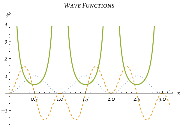
Figure 1: The ground state (dotted line) and first excited state (dashed line) wave functions in $V_{2}(x)=2\csc^{2}(x)-1$ have been plotted. We assume that $L=\pi$.

3 Generalized Uncertainty Principle

The GUP, which stands for the Generalized Uncertainty Principle, is an extension of the famous Heisenberg Uncertainty Principle in quantum mechanics. The Heisenberg Uncertainty Principle states that there is a fundamental limit to the precision with which certain pairs of physical properties, such as position and momentum, can be simultaneously known. However, the Generalized Uncertainty Principle goes a step further by considering the effects of gravity.
The Generalized Uncertainty Principle arises from attempts to reconcile quantum mechanics with general relativity, which describes gravity as the curvature of spacetime caused by mass and energy. In the context of GUP, the uncertainty in position and momentum is modified to include gravitational effects.
Mathematically, the Generalized Uncertainty Principle can be expressed in various forms, depending on the specific theoretical framework being used. One common form is.

(16) $$\Delta x\Delta p\geq\frac{\hbar}{2}[1+\alpha\Delta x^{2}+\beta\Delta p^{2}]$$

Here, $\Delta x$ represents the uncertainty in position, $\Delta p$ represents the uncertainty in momentum, $\hbar$ is the reduced Planck constant, and $\alpha$ and $\beta$ are dimensionless parameters that depend on the specific theory being considered. These parameters are typically associated with the effects of gravity.
The Generalized Uncertainty Principle introduces additional terms involving the squares of the uncertainties in position and momentum, which are not present in the Heisenberg Uncertainty Principle. These terms reflect the influence of gravity on the fundamental limits of measurement in quantum mechanics.
It is important to note that the Generalized Uncertainty Principle is still an area of active research and is not yet fully understood. Different theoretical frameworks, such as string theory and loop quantum gravity, may yield different forms of the Generalized Uncertainty Principle (GUP). Therefore, the specific mathematical relationships of the Generalized Uncertainty Principle (GUP) can vary depending on the theoretical context in which it is applied. So, the commutator relation between $\hat{x}$ and $\hat{p}$ is:

(17) $$[\hat{X},\hat{P}]=i\hbar(1+\alpha\hat{x}^{2}+\beta\hat{p}^{2})$$

Let us define the generalized space and momentum operators

(18) $$\hat{X}=x$$

(19) $$\hat{P}=-i\hbar[(1+\alpha x^{2})\frac{d}{dx}+\gamma x]$$

Now we are going to investigate supersymmetries in quantum mechanics using generalized operators of space and momentum.[10, 11, 12]

4 Generalized supersymmetry in quantum mechanics

Let’s obtain the Hamiltonian in this approach, so

$$\hat{\tilde{H}} =\hat{P}^{2}+V(x)$$

$$=-(1+\alpha x^{2})^{2}\frac{d^{2}}{dx^{2}}-2(\gamma+\alpha)x(1+\alpha x^{2})\frac{d}{dx}$$

(20) $$-\gamma(1+\alpha x^{2})-\gamma^{2}x^{2}+V(x)$$

we assume $i\hbar=1$ , so the Hamiltonian is Hermitian and the normalized wave functions in $\mathcal{H}ilbert\;space\;(a,b)$ is as[13],[14]

(21) $$\bra{\psi_{n}}\ket{\psi_{m}}=\int^{b}_{a}\frac{\psi^{*}_{n}(x)\psi_{m}(x)}{1+\alpha x^{2}}dx$$

We prove this in Appendix A. In this case we define the generalized potential $\tilde{V}(x)$ which $\tilde{V}(\alpha,\gamma;x)=V(x)-\gamma(1+\alpha x^{2})-\gamma^{2}x^{2}$ . Let us define the generalized creation and annihilation operators

(22) $$\hat{\tilde{A}}=(1+\alpha x^{2})\frac{d}{dx}+\gamma x+\tilde{W}(x)$$

(23) $$\hat{\tilde{A}}^{\dagger}=-(1+\alpha x^{2})\frac{d}{dx}-\gamma x+\tilde{W}(x)$$

where $\tilde{W}(x)$ is Generalized Superpotential. Now we can construct the Hamiltonian Super partner by creation and annihilation operators like sections II, so

(24) $$\hat{\tilde{H}}_{1}=\hat{\tilde{A}}^{\dagger}\hat{\tilde{A}}\;\;,\;\;\hat{\tilde{H}}_{2}=\hat{\tilde{A}}\hat{\tilde{A}}^{\dagger}$$

and we have yet this relations

(25) $$\hat{\tilde{A}}\hat{\tilde{H}}_{1}=\hat{\tilde{H}}_{2}\hat{\tilde{A}}\;\;,\;\;\hat{\tilde{H}}_{1}\hat{\tilde{A}}^{\dagger}=\hat{\tilde{A}}^{\dagger}\hat{\tilde{H}}_{2}$$

therefore

(26) $$V_{1}(x)=\tilde{W}^{2}(x)-(1+\alpha x^{2})\tilde{W}^{{}^{\prime}}(x)$$

(27) $$V_{2}(x)=\tilde{W}^{2}(x)+(1+\alpha x^{2})\tilde{W}^{{}^{\prime}}(x)$$

and

(28) $$\psi^{2}_{n}(x)=\hat{\tilde{A}}\psi^{1}_{n+1}(x)\;\;,\;\;\psi^{1}_{n+1}(x)=\hat{\tilde{A}}^{\dagger}\psi^{2}_{n}(x)$$

(29) $$\tilde{E}^{2}_{n}=\tilde{E}^{1}_{n+1}\;\;,\;\;\tilde{E}^{1}_{0}=0$$

Therefore, potentials do not depend on $\gamma$, but wave functions and generalized potentials do depend on $\gamma$.
Now, considering the ground state wave function has zero energy, we can write it as eq. 8.

$$\hat{\tilde{A}}\psi^{1}_{0}(x)=[(1+\alpha x^{2})\frac{d}{dx}+\gamma x+\tilde{W}(x)]\psi^{1}_{0}(x)=0$$

(30) $$\tilde{W}(x)=-(1+\alpha x^{2})\frac{\psi^{1^{\prime}}_{0}(x)}{\psi^{1}_{0}(x)}-\gamma x$$

So we can obtain $\tilde{W}(x)$ by using the ground state wave functions of the first system, $\hat{H}_{1}$. We can then generate multiple potentials and their corresponding solutions.
Now, the problem that exists is that a wide range of generalized Hamiltonians cannot be solved analytically or numerically. To utilize supersymmetry, we need to obtain the solution for one of the systems. However, the difficulty in finding a solution hinders this work.
An analytical method is used to find solutions for the generalized system by using the classical system. In this situation, we use perturbation theory. In the next section, we will discuss the analytical solution of the generalized Hamiltonian using perturbation theory.

5 Analytical solution of generalized Hamiltonian by perturbation theory

In this section, we attempt to find approximate solutions for the generalized Hamiltonian using perturbation theory[15, 16, 17] and classical Hamiltonian solutions. Considering that we are using perturbation theory, we consider $\alpha$ as the perturbation factor. At first, we establish a relationship between the classical and generalized creation and annihilation operators. This creates a connection between the classical and generalized superpotential. Let us assume that $\gamma=0$.

(31) $$\tilde{W}(x)=(1+\alpha x^{2})W(x)$$

(32) $$\hat{\tilde{A}}=(1+\alpha x^{2})\frac{d}{dx}+\tilde{W}(x)=(1+\alpha x^{2})\hat{A}$$

(33) $$\hat{\tilde{A}}^{\dagger}=-(1+\alpha x^{2})\frac{d}{dx}+\tilde{W}(x)=(1+\alpha x^{2})\hat{A}^{\dagger}$$

Therefore from eq.24 for $\hat{\tilde{H}}_{1}$ we have

$$\hat{\tilde{H}}_{1} =\hat{\tilde{A}}^{\dagger}\hat{\tilde{A}}=(1+\alpha x^{2})\hat{A}^{\dagger}(1+\alpha x^{2})\hat{A}$$

$$=(1+\alpha x^{2})^{2}\hat{A}^{\dagger}\hat{A}-2\alpha x(1+\alpha x^{2})\frac{d}{dx}$$

(34) $$=(1+\alpha x^{2})^{2}\hat{H}_{1}-2\alpha x(1+\alpha x^{2})\frac{d}{dx}$$

Considering the $O(\alpha^{3})$ becomes very small, from perturbation theory we have

(35) $$\hat{\tilde{H}}_{1}=\hat{H}_{1}+\alpha\hat{H^{1}}+\alpha^{2}\hat{H^{2}}$$

where

(36) $$\hat{H^{1}}=2x^{2}\hat{H}_{1}-2x\frac{d}{dx}\;\;,\;\;\hat{H^{2}}=x^{4}\hat{H}_{1}-2x^{3}\frac{d}{dx}$$

so the wave functions and energy levels are

(37) $$\hat{\tilde{H}}_{1}\tilde{\psi}^{1}_{n}(x)=\hat{\tilde{E}}_{1}\tilde{\psi}^{1}_{n}(x)$$

(38) $$\psi^{1}_{n}(x)=\phi^{1}_{n}(x)+\alpha\phi^{1,1}_{n}(x)+\alpha^{2}\phi^{1,2}_{n}(x)$$

(39) $$\tilde{E}^{1}_{n}=E^{1}_{n}+\alpha E^{1,1}_{n}+\alpha^{2}E^{1,2}_{n}$$

that

(40) $$\phi^{1,1}_{n}(x)=\sum_{m\neq n}\frac{H^{1}_{mn}}{E^{1}_{n}-E^{1}_{m}}\bra{x}\ket{\phi^{1}_{m}}$$

$$\phi^{1,2}_{n}(x)=\sum_{m\neq n}\frac{1}{E^{1}_{n}-E^{1}_{m}}[H^{2}_{mn}+h^{1}_{mn}$$

(41) $$-\frac{E^{1,1}_{n}}{E^{1}_{n}-E^{1}_{m}}H^{1}_{mn}]\bra{x}\ket{\phi^{1}_{m}}$$

(42) $$E^{1,1}_{n}=\bra{\phi^{1}_{n}}\hat{H}^{1}\ket{\phi^{1}_{n}}$$

(43) $$E^{1,2}_{n}=\bra{\phi^{1}_{n}}\hat{H}^{2}\ket{\phi^{1}_{n}}+\sum_{m\neq n}\frac{\absolutevalue{H^{1}_{mn}}^{2}}{E^{1}_{n}-E^{1}_{m}}$$

where

(44) $$H^{2}_{mn}=\bra{\phi^{1}_{m}}\hat{H}^{2}\ket{\phi^{1}_{n}}$$

(45) $$H^{1}_{mn}=\bra{\phi^{1}_{m}}\hat{H}^{1}\ket{\phi^{1}_{n}}$$

(46) $$h^{1}_{mn}=\bra{\phi^{1}_{m}}\hat{H}^{2}\ket{\phi^{1}_{n}}=\sum_{k\neq n}\frac{H^{1}_{kn}H^{1}_{mk}}{E^{1}_{n}-E^{1}_{k}}$$

where $\phi^{1}_{n}(x)$ and $E^{1}_{n}$ are wave functions and energy levels for the classical Hamiltonian $\hat{H}_{1}$, respectively. As it is known, in this method, $\gamma=0$.
As mentioned earlier, the analytical solution is obtained using perturbation theory. It relies on the perturbation factor and the degree to which we utilize it. Therefore, these solutions are not exact, and the accuracy of the answers increases as we assume a higher degree of the perturbation factor, denoted by $\alpha$. Analytical solutions are obtained, but the advantage of these solutions is that they can be used in cases where it is not feasible to solve the generalized Schrödinger equation, which is dependent on the Hamiltonian, using numerical methods. Therefore, the analytical method helps solve such problems. In the next section, we will examine two famous examples in quantum mechanics and compare the accuracy of analytical and numerical solutions.

6 Examples

In this section, we will solve two well-known examples in quantum mechanics for a generalized Hamiltonian using numerical and analytical methods. The first one is the particle in a box, and the second one is the harmonic oscillator. As mentioned, the numerical method refers to solutions obtained through programming codes and relevant software. In section V, we derive the condition for the analytical method, which is $\gamma=0$.

6.1 Particle in a box

In the example of a particle in a box, we know that the wave function and energy levels in the classical Hamiltonian are as follows.

(47) $$\phi_{n}(x)=\sqrt{\frac{2}{L}}sin(\frac{n\pi x}{L})\;\;,\;\;E_{n}=\frac{n^{2}\pi^{2}}{2mL^{2}}$$

First, we solve the generalized particle in a box problem. Then, we obtain the superpotential and generate potentials to find the wave functions and energy levels.

6.1.1 Numerical solution

In this case, the generalized Hamiltonian is

(48) $$\hat{H}=-(1+\alpha x^{2})^{2}\frac{d^{2}}{dx^{2}}-2\alpha x(1+\alpha x^{2})\frac{d}{dx}$$

Let we assume $L=\pi$ then the normal wave functions and energy levels are

(49) $$\psi^{1}_{n}(x)=\bigg{[}\frac{2\sqrt{a}}{tan^{-1}(\sqrt{a}\pi)}\bigg{]}^{1/2}sin\bigg{[}\frac{n\pi tan^{-1}(\sqrt{a}x)}{tan^{-1}(\sqrt{a}\pi)}\bigg{]}$$

(50) $$\tilde{E}_{n}=\frac{an^{2}\pi^{2}}{[tan^{-1}(\pi\sqrt{a})]^{2}}$$

In the limit as $\alpha\rightarrow 0$, the wave functions and energy levels correspond to the classical case described by equation 47. Therefore, we can determine the wave functions and energy levels for the generalized Hamiltonian of a particle in a box. In Figure 2, the ground and first excited states are plotted for $\alpha=0.2$.

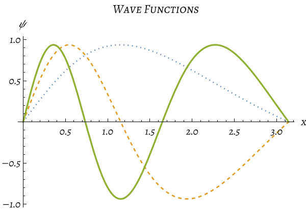
Figure 2: The ground (dotted line), first (dashed line), and second (thick line) excited states of wave functions for the generalized Hamiltonian of a particle in a box for $\alpha=0.2$. As you can see, the wave function deviates from its classical state and shifts to the left as the value of $\alpha$ increases. We assume that $L=\pi$.

Now, by obtaining the wave functions and energy levels for the generalized particle-in-a-box problem, we can solve the partner potential using generalized supersymmetry. So, from equation 30, we have

(51) $$\tilde{W}(x)=-\frac{\pi\sqrt{a}}{tan^{-1}(\pi\sqrt{a})}cot[\frac{\pi tan^{-1}(\pi\sqrt{x})}{tan^{-1}(\pi\sqrt{a})}]$$

then from eq.27

$$V_{2}(x) =\frac{a\pi^{2}}{[tan^{-1}(\pi\sqrt{a})]^{2}}\bigg{[}2\csc^{2}[\frac{\pi tan^{-1}(\pi\sqrt{x})}{tan^{-1}(\pi\sqrt{a})}]-1\bigg{]}$$

(52) $$+\frac{2\pi a^{5/2}x^{3}cot[\frac{\pi tan^{-1}(\pi\sqrt{x})}{tan^{-1}(\pi\sqrt{a})}]}{tan^{-1}(\pi\sqrt{a})}$$

so the wave functions from eq.28 are

(53) $$\psi^{2}_{1}(x) =-\frac{2\sqrt{a}\pi}{tan^{-1}(\pi\sqrt{a})}\sin^{2}\bigg{[}\frac{\pi tan^{-1}(\sqrt{a}x)}{tan^{-1}(\sqrt{a}\pi)}\bigg{]}$$

$$\psi^{2}_{2}(x) =-\frac{8\sqrt{a}\pi}{tan^{-1}(\pi\sqrt{a})}\sin^{2}\bigg{[}\frac{\pi tan^{-1}(\sqrt{a}x)}{tan^{-1}(\sqrt{a}\pi)}\bigg{]}$$

(54) $$\cos[\frac{\pi tan^{-1}(\sqrt{a}x)}{tan^{-1}(\sqrt{a}\pi)}\bigg{]}$$

$$\vdots$$

and the energy levels are

(55) $$\tilde{E}^{2}_{1}=\frac{a\pi^{2}}{[tan^{-1}(\pi\sqrt{a})]^{2}}$$

(56) $$\tilde{E}^{2}_{2}=\frac{4a\pi^{2}}{[tan^{-1}(\pi\sqrt{a})]^{2}}$$

$$\vdots$$

Therefore, using generalized supersymmetry, we were able to solve the potentials generated by the particle potential in a box in the generalized quantum mechanical framework. We must consider that in the limiting case where $\alpha\rightarrow 0$, the solutions of the potentials tend to their classical state. As seen in Figure 3, we plotted the wave functions for the ground state and first excited state of $V_{2}(x)$ with $\alpha=0.1$.
In Figure 4, we plot the energy levels in the generalized Hamiltonian and classical Hamiltonian for $\alpha=0,0.01,0.1$.
Therefore, we obtain wave functions and energy levels in potentials generated by the particle in a box potential in generalized quantum mechanics through the use of generalized supersymmetry (GSUSYQM).

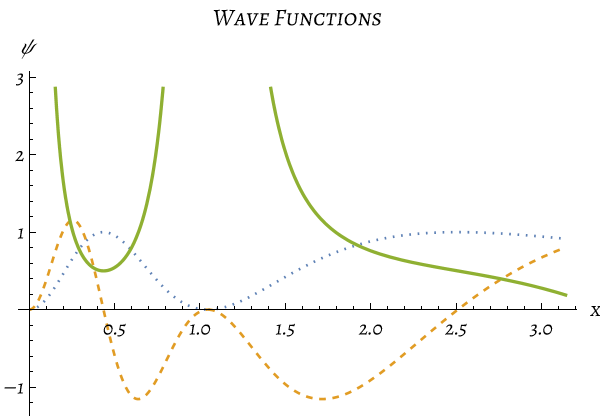
Figure 3: In this figure, we assume that $\alpha=0.1$. The thick line represents $V_{2}(x)$ from equation 40, the dotted line represents the ground state wave function, and the dashed line represents the excited state wave function. We consider $L=\pi$. If $\alpha\rightarrow 0$, we refer to Figure 1.

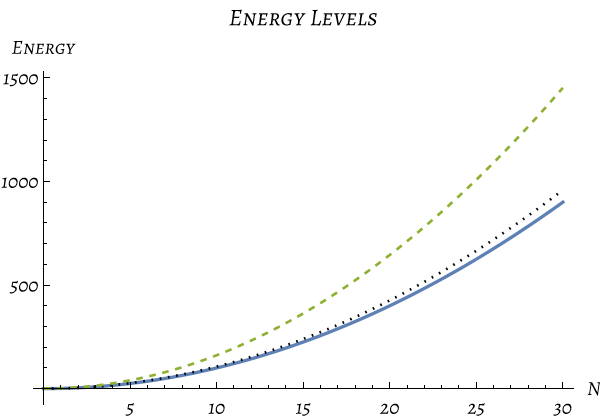
Figure 4: In this figure, we examined the behavior of energy levels in terms of different $\alpha$ and nth levels. We plotted for different values of $\alpha$, where the thick line represents $\alpha=0$ (classic), the dotted line represents $\alpha=0.01$, and the dashed line represents $\alpha=0.1$. As you can see, as the value of $\alpha$ approaches 0, the energy levels converge to the classical states.

6.1.2 Analytical solution

Let’s solve the generalized particle in a box using perturbation theory. We assume $O(\alpha^{2})\rightarrow 0$. According to Section V, we can solve this generalized Hamiltonian using a convenient approximation. Therefore, from equations 38,39,40and 42, we have

$$\bra{\phi^{1}_{m}}\hat{H}\ket{\phi^{1}_{n}}=H_{mn} =2n[\frac{m+n}{(m-n)^{2}}(-1)^{m-n}$$

(57) $$+\frac{m-n}{(m+n)^{2}}(-1)^{m+n}]$$

and

(58) $$\bra{\phi^{1}_{n}}\hat{H}\ket{\phi^{1}_{n}}=\frac{2\pi^{2}n^{2}}{3}$$

then the wave functions and energy levels are

(59) $$\psi^{1}_{n}(x)=\sqrt{\frac{2}{\pi}}\bigg{[}\sin(nx)+\alpha\sum_{m\neq n}\frac{H_{mn}}{n^{2}-m^{2}}\sin(mx)\bigg{]}$$

(60) $$\tilde{E}^{1}_{n}=n^{2}+\alpha\frac{2\pi^{2}n^{2}}{3}$$

In Figure 5, the ground state and first excited state wave functions have been plotted for $\alpha=0.2$. As it is known, the wave function leads to the exact solution through the analytical solution method when $\alpha\rightarrow 0$. By considering higher order terms such as $\alpha^{2},\alpha^{3},\dots$, our solution becomes more accurate.

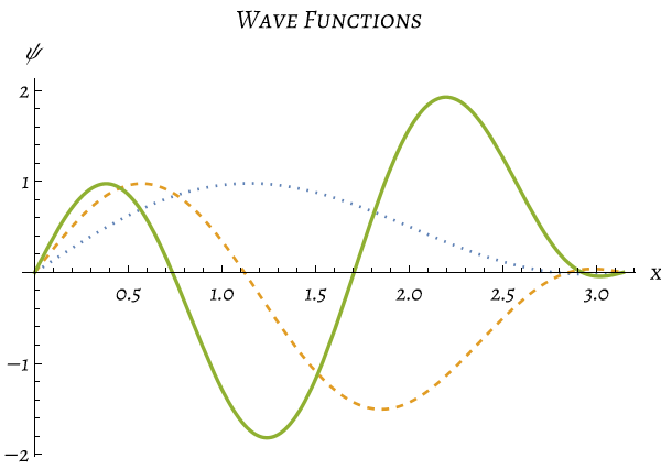
Figure 5: The ground (dotted line), first (dashed line), and Second excited state wave functions for the generalized Hamiltonian of a particle in a box for $\alpha=0.2$ using the analytical method. As shown, the analytical method is a good approximation for solving the generalized Hamiltonian.

In Figure 6, we plot energy levels for $\alpha=0.01$ and $\alpha=0.1$. As shown, for $\alpha=0.01$, the energy levels of the solution are exact. However, for the approximation of $\alpha=0.1$, there is a quantitative difference from the exact solution.

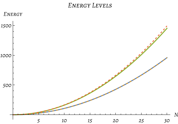
Figure 6: In this figure, we plotted energy levels using both analytical and numerical methods for different values of $\alpha$. The thick lines represent the numerical results, with the bottom line corresponding to $\alpha=0.01$ and the upper line corresponding to$\alpha=0.1$. The dashed lines represent the analytical results, with the bottom line also corresponding to $\alpha=0.01$ and the upper line corresponding to $\alpha=0.1$. As shown, the difference in energy levels between numerical and analytical methods when $\alpha<<1$ is very small.

Now, if we want to obtain the partner potentials of the particle potential in a box through generalized supersymmetry from eq.30 and the ground state wave function, we have.

(61) $$\psi^{1}_{1}(x)=\sqrt{\frac{2}{\pi}}\bigg{[}\sin(x)+\alpha\sum_{m\neq 1}\frac{H_{m1}}{1-m^{2}}\sin(mx)\bigg{]}$$

(62) $$\tilde{W}(x.m)=-(1+\alpha x^{2})\frac{\cos(x)+\alpha\sum_{m\neq 1}\frac{mH_{m1}}{1-m^{2}}\cos(mx)}{\sin(x)+\alpha\sum_{m\neq 1}\frac{H_{m1}}{1-m^{2}}\sin(mx)}$$

or from eq.31

(63) $$\tilde{W}(x)=-(1+\alpha x^{2})\cot(x)$$

In fact, these two superpotential are the same , $\lim_{m\rightarrow\infty}\tilde{W}(x,m)=\tilde{W}(x)$.
So the second potential is

(64) $$V_{2}(x)=(1+ax^{2})[2\csc^{2}(x)-1]-2ax(1+ax^{2})\cot(x)$$

Now, from eq.32 and 33, we can obtain the wave functions in this potential.

(65) $$\psi^{2}_{1}(x)=\hat{\tilde{A}}\psi^{1}_{2}(x)=(1+\alpha x^{2})\hat{A}\psi^{1}_{2}(x)$$

(66) $$\psi^{2}_{2}(x)=\hat{\tilde{A}}\psi^{1}_{3}(x)=(1+\alpha x^{2})\hat{A}\psi^{1}_{3}(x)$$

$$\vdots$$

As shown in Figure 7, the wave functions for the ground state and first excited state have been plotted for $\alpha=0.2$.

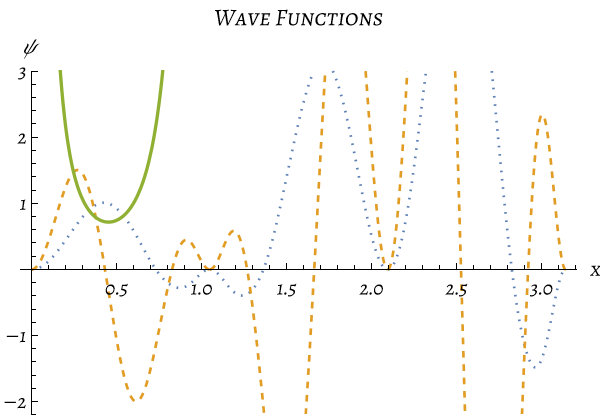
Figure 7: In this figure, we assume $\alpha=0.1$ and the thickness. The solid-state function, while the dashed represents the state. state Wave we arrive at Figure 3.

As expected, perturbation theory provides approximate but accurate solutions for wave functions and energy levels in generalized systems. Therefore, we can first use their classical form to solve difficult generalized Hamiltonians and then apply perturbation theory to obtain wave functions and energy levels for the potentials generated from them through generalized supersymmetry.

6.2 Harmonic oscillator

As we know, the wave function and energy values for a harmonic oscillator are as follows

(67) $$\phi_{n}(x)=\frac{1}{\sqrt{2^{n}n!}}(\frac{m\omega}{\pi\hbar})^{1/4}e^{-\frac{m\omega x^{2}}{2\hbar}}\mathcal{H}_{n}(\sqrt{\frac{m\omega}{\hbar}x)}$$

(68) $$E_{n}=\hbar\omega(n+\frac{1}{2})$$

In supersymmetry in quantum mechanics, it is necessary to consider a gap between the two potentials to account for the superpotential, wave functions, and energy levels [4].

(69) $$W(x)=\frac{1}{2}\omega x-b$$

(70) $$V_{1}(x)=\frac{1}{4}\omega^{2}(x-\frac{2b}{\omega})^{2}-\frac{\omega}{2}$$

(71) $$E^{1}_{n}=n\omega$$

(72) $$\phi^{1}_{n}(x)\propto\exp(-\frac{1}{2}y^{2})\mathcal{H}_{n}(y)$$

where

(73) $$y=\sqrt{\frac{\omega}{2}}(x-\frac{2b}{\omega})$$

Now we obtain the wave functions and energy levels for the generalized harmonic oscillator using numerical and analytic methods.

6.2.1 Numerical solution

Let’s obtain the wave functions in the Generalized Harmonic Oscillator. The Generalized Hamiltonian for this case is known

(74) $$\hat{H}=-(1+\alpha x^{2})^{2}\frac{d^{2}}{dx^{2}}-2\alpha x(1+\alpha x^{2})\frac{d}{dx}+\frac{1}{4}x^{2}-\frac{1}{2}$$

so the wave function in numerical solution is

(75) $$\psi^{1}_{n}(x)=c_{1}P^{(-\frac{1}{2}+\sqrt{\frac{-2+a^{2}}{4a^{2}}})}_{\frac{\sqrt{-1+2ae}}{\sqrt{2}a}}(x)+c_{2}Q^{(-\frac{1}{2}+\sqrt{\frac{-2+a^{2}}{4a^{2}}})}_{\frac{\sqrt{-1+2ae}}{\sqrt{2}a}}(x)$$

where $P^{m}_{n}(x)$ and $Q^{m}_{n}(x)$ are associated Legendre functions and is defined

$$P^{m}_{n}(x)=\frac{1}{\Gamma(1-m)}[\frac{1+x}{1-x}]^{m/2}$$

(76) $$F_{1}(-n,n+1;1-m;\frac{1-x}{2})$$

$$Q^{m}_{n}(x)=\frac{\sqrt{\pi}\Gamma(1+n+m)}{2^{n+1}\Gamma(1-m)}\frac{(1-x^{2})^{m/2}}{x^{m+n+1}}$$

(77) $$F_{1}(\frac{m+n+1}{2},\frac{m+n+2}{2};n+\frac{3}{2};\frac{1}{x^{2}})$$

where

(78) $$F_{1}(\alpha,\beta;\gamma;z)=\frac{\Gamma(\gamma)}{\Gamma(\alpha)\Gamma(\beta)}\sum^{\infty}_{n=0}\frac{\Gamma(\alpha+n)\Gamma(\beta+n)}{\Gamma(\gamma+n)n!}z^{n}$$

is called hypergeometric functions.[18, 19, 14]
According to eq.75, it is very difficult to use this wave function to check and obtain energy levels. Therefore, this numerical solution is not as useful as it should be. Therefore, we use the analytical method of perturbation theory.

6.2.2 Analytical solution

We want to obtain the ground state wave function and energy level for a generalized Hamiltonian. For the classical Hamiltonian, the ground state, first excited state, and second excited state wave functions and energy levels are as follows

(79) $$\phi^{1}_{0}(x)=\frac{1}{\pi^{1/4}}e^{-\frac{x^{2}}{2}}\;\;,\;\;E_{0}=2$$

(80) $$\phi^{1}_{1}(x)=\frac{2}{\pi^{1/4}}xe^{-\frac{x^{2}}{2}}\;\;,\;\;E_{0}=4$$

(81) $$\phi^{1}_{2}(x)=\frac{2}{\pi^{1/4}}(2x^{2}-1)e^{-\frac{x^{2}}{2}}\;\;,\;\;E_{0}=6$$

For convenience we assume $\omega=2$ and $b=0$. Now, the ground state wave function and energy level for the generalized Hamiltonian from eqs.40 and 42 are:

(82) $$\bra{\phi^{1}_{m}}\hat{H}\ket{\phi^{1}_{0}}=\frac{5}{\sqrt{\pi}}\int^{\infty}_{-\infty}x^{2}\mathcal{H}_{m}(x)e^{-x^{2}}dx$$

and for the ground state energy

(83) $$\bra{\phi^{1}_{0}}\hat{H}\ket{\phi^{1}_{0}}=\frac{5}{4}$$

so the ground state wave functions generalized Harmonic oscillator are

$$\psi^{1}_{0}(x) =\frac{1}{\pi^{1/4}}\bigg{[}e^{-\frac{x^{2}}{2}}$$

(84) $$-\alpha\frac{5}{\pi^{1/4}}\sum_{m\neq 0}\frac{1}{m}\int^{\infty}_{-\infty}x^{2}\mathcal{H}_{m}(x)e^{-x^{2}}dx\phi^{1}_{m}(x)\bigg{]}$$

and the ground state, first and second excited states’ energy levels

(85) $$\tilde{E}^{1}_{0}=2+\alpha\frac{5}{4}$$

(86) $$\tilde{E}^{1}_{1}=4+\alpha\frac{25}{4}$$

(87) $$\tilde{E}^{1}_{2}=6+\alpha\frac{65}{4}$$

In figures 8 and 9, the ground state wave function and energy levels for the generalized harmonic oscillator have been plotted, respectively.
On the other hand, in Figure 10, the ground, first, and second excited states are plotted for $\alpha=0.1$. As we expect, if $\alpha\rightarrow 0$, then the wave function tends to the classical wave function. Pay attention that we have omitted the higher degrees of $\alpha$, and the accuracy of the wave functions and energy levels is related to the perturbation factor $(\alpha)$.
Now, from eq.31, we can obtain the generalized superpotential. Then, using eqs.32 and 33, one can derive the wave function and energy levels for newer potentials. The potentials are as follows:

(88) $$V_{1}(x)=x^{2}(1+ax^{2})^{2}-(1+ax^{2})(1+3ax^{2})$$

(89) $$V_{2}(x)=x^{2}(1+ax^{2})^{2}+(1+ax^{2})(1+3ax^{2})$$

The equation 84 represents the ground state wave function of the potential $V_{1}(x)$, while equations 85, 86, and 87 represent the energy levels for the ground state, first excited state, and second excited state of the respective potentials.
Now, from Eq. (28) and (32), we can obtain the wave functions of the potential $V_{2}(x)$. So, the wave functions of the ground and first excited states, $\dots$, are.

$$\psi^{2}_{1}(x)=\hat{\tilde{A}}\psi^{1}_{2}(x)=(1+\alpha x^{2})\hat{A}\psi^{1}_{2}(x)$$

$$\psi^{2}_{2}(x)=\hat{\tilde{A}}\psi^{1}_{3}(x)=(1+\alpha x^{2})\hat{A}\psi^{1}_{3}(x)$$

$$\vdots$$

$$\psi^{2}_{n}(x)=\hat{\tilde{A}}\psi^{1}_{n+1}(x)=(1+\alpha x^{2})\hat{A}\psi^{1}_{n+1}(x)$$

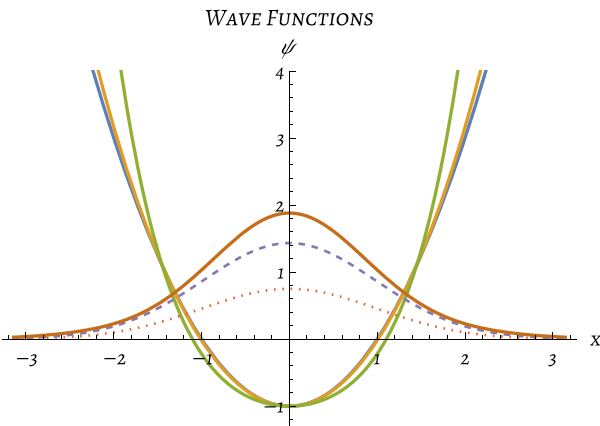
Figure 8: As shown, the ground state wave functions in potentials $V_{2}(x)$ for $\alpha=0,0.1,0.1$ have been plotted using dotted, dashed, and thick lines, respectively. As we expected, if$\alpha\rightarrow 0$, then the wave function will be the classical ground state wave function (dotted line).

In Figure 11, the ground, first, and excited states for $\alpha=0.1$ have been plotted. As it is known if $\alpha\rightarrow 0$, then the figures 10 and 11 are the same. This can be used to verify the correctness of our answer. On the other hand, if we consider intuition and the classical point of view, we can observe that potential $V_{2}(x)$ is wider than potential $V_{1}(x)$. Classically, this width causes a perturbation in the wave. Comparing it to Figure 10, we can see that the wave at that point should change the domain. This perturbation and change can be observed in Figure 11.

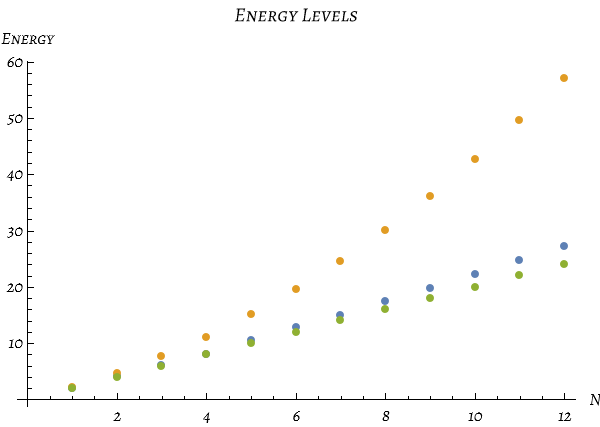
Figure 9: In this figure, the energy levels for different $\alpha$ are plotted. The bottom line represents $\alpha=0$, the middle line represents $\alpha=0.01$, and the upper line represents $\alpha=0.1$. As $\alpha$ approaches zero, the energy levels will converge to the classical energy levels.

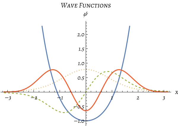
Figure 10: As shown in the graph, the ground state, first excited state, and second excited state wave functions for $\alpha=0.1$ have been plotted using dotted, dashed, and thick lines, respectively. As we expected, if $\alpha$ approaches 0, then the wave functions will resemble Figure 10.

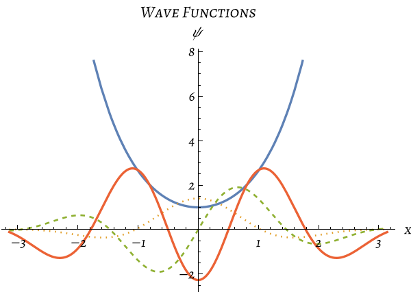
Figure 11: In this figure, the ground state, first, and second excited wave functions in $V_{2}(x)$ for $\alpha=0.1$ are plotted using dotted, dashed, and thick lines, respectively.

7 conclusion

In summary, first we will review supersymmetry in quantum mechanics and solve the new potentials generated from the infinite square well potential. Then, we describe the Generalized Uncertainty Principle (GUP) and consider the new form of the momentum operator eq.19. Next, we investigate the concept of supersymmetry in quantum mechanics using GUP, or in other words, the Generalized Supersymmetry in quantum mechanics. We explore the existence of supersymmetry in this form.
In the following, since it can be challenging to solve the generalized Hamiltonian directly in certain systems, we utilized perturbation theory to solve it. This approach established relationships between the creation and annihilation operators and allowed us to solve two well-known examples. For the second example, which involved the harmonic oscillator, solving it numerically proved to be quite challenging. This led us to appreciate the advantages of the analytical solution. By employing this method, we were able to obtain the Hamiltonian solution for the generalized harmonic oscillator.
So, we construct supersymmetry in quantum mechanics using the generalized uncertainty principle (GUP) and obtain analytical solutions to solve generalized Hamiltonians. Through this approach, we generate many potentials using generalized supersymmetry, allowing us to obtain wave functions and energy levels in a generalized form.

Appendix A

First, let us define the Adjoint Differential Operators. Consider we have the operator differential as

(90) $$\hat{\mathcal{L}}=p_{2}(x)\frac{d^{2}}{dx^{2}}+p_{1}(x)\frac{d}{dx}+p_{0}(x)$$

and we have the differential equation

(91) $$\hat{\mathcal{L}}[u]\equiv p_{2}(x)\frac{d^{2}u}{dx^{2}}+p_{1}(x)\frac{du}{dx}+p_{0}(x)u=0$$

Now let us define some definitions and propositions.
Difinition 1  The eq.91 is said to be exact if

(92) $$p_{2}(x)\frac{d^{2}u}{dx^{2}}+p_{1}(x)\frac{du}{dx}+p_{0}(x)u=\frac{d}{dx}[A(x)u^{{}^{\prime}}+B(x)u]$$

for all $u\in\mathcal{H}^{2}[a,b]$ and for some $A,B\in\mathcal{H}[a,b]$. An integrating factor for $\hat{\mathcal{L}}[u]$ is a function $\mu(x)$ such that $\mu(x)\hat{\mathcal{L}}[u]$ is exact[14].
Proposition 1  A function $\mu(x)$ is an integrating factor of the eq.91 if and only if it is a solution for

(93) $$\hat{\mathcal{M}}[\mu]\equiv(p_{2}\mu)^{{}^{\prime\prime}}-(p_{1}\mu)^{{}^{\prime}}+p_{0}\mu=0$$

The operator $\hat{\mathcal{M}}$ given by

(94) $$\hat{\mathcal{M}}\equiv p_{2}\frac{d^{2}}{dx^{2}}+(2p_{2}-p_{1})\frac{d}{dx}+(p^{{}^{\prime\prime}}_{2}-p^{{}^{\prime}}_{1}-p_{0})$$

is called the adjoint of the operator $\hat{\mathcal{L}}$ and denoted by $\hat{\mathcal{M}}\equiv\hat{\mathcal{L}}^{\dagger}$[14].
Theorem 1  The eq.91 is self-adjoint(Hermitian) if and only if $p^{{}^{\prime}}_{2}=p_{0}$ in which the eq.91 can be written

(95) $$\frac{d}{dx}[p_{2}(x)\frac{du}{dx}]+p_{0}u=0$$

If it is not self-adjoint, it can be made so by multiplying it through by

(96) $$\mu(x)=\frac{1}{p_{2}(x)}\exp[\int^{x}\frac{p_{1}(t)}{p_{2}(t)}dt]$$

Now we know when an operator is an adjoint or self-adjoint. Now we will examine the orthogonality of the solutions of a differential equation.
From Sturm-Liouville systems[14, 20] and second order differential equations(SOLDEs) , assume $\hat{\mathcal{L}}$ is an operator(not self-adjoint), then if we have eigenvalue problem(differential equation) as

(97) $$\hat{\mathcal{L}}[u]+\lambda[u]=0$$

which can be written

(98) $$p_{2}(x)\frac{d^{2}u}{dx^{2}}+p_{1}(x)\frac{du}{dx}+p_{0}(x)u+\lambda u=0$$

From Theorem 1 , by multiplying integrating factor the $\hat{\mathcal{L}}$ be self-adjoint and we have

(99) $$\frac{d}{dx}[p(x)\frac{du}{dx}]+[\lambda\mu(x)-q(x)]u=0$$

where $p(x)=\mu(x)p_{2}(x)$ and $q(x)=-\mu(x)p_{0}(x)$.
Now from Lagrange identity for a self-adjoint differential operator $\hat{\mathcal{L}}$ [14, 21]

(100) $$u\hat{\mathcal{L}}[v]-v\hat{\mathcal{L}}[u]=\frac{d}{dx}[p(x)[u(x)v^{{}^{\prime}}(x)-v(x)u^{{}^{\prime}}(x)]]$$

which $u(x)$ and $v(x)$ are the solution of eq.99 and if $\lambda_{1}$ and $\lambda_{2}$ are the eigenvalue of eq.97 , respectively, so

(101) $$u\hat{\mathcal{L}}[v]-v\hat{\mathcal{L}}[u]=(\lambda_{1}-\lambda_{2})\mu(x)u(x)v(x)$$

Integrating both sides of eq.101 then yields

(102) $$(\lambda_{1}-\lambda_{2})\int^{b}_{a}\mu uvdx=p(x)[u(x)v^{{}^{\prime}}(x)-v(x)u^{{}^{\prime}}(x)]|^{b}_{a}$$

now if $u(x)$ and $v(x)$ could satisfy the boundary condition that the Sturm-Liouville system defined, then the inner product integral with weight function(or integrating factor) $\mu(x)$ is

(103) $$\bra{u}\ket{v}\equiv\int^{b}_{a}\mu(x)u(x)v(x)dx$$

Let check eqs.20 and 22. We know the Hamiltonian from eq.20 is hermitian , so it is self-adjoint and from eqs.96 and 103 the inner product for wave functions of Hamiltonian is

(104) $$\bra{\psi_{n}}\ket{\psi_{m}}=\int^{b}_{a}\frac{\psi^{*}_{n}(x)\psi_{m}(x)}{1+\alpha x^{2}}dx$$

References

- [1] Jun-Li Li and Cong-Feng Qiao. The generalized uncertainty principle. Annalen der Physik, 533(1), November 2020.
- [2] Roberto Casadio and Fabio Scardigli. Generalized uncertainty principle, classical mechanics, and general relativity. Physics Letters B, 807:135558, August 2020.
- [3] B Bagchi, R Ghosh, and P Goswami. Generalized uncertainty principle and momentum-dependent effective mass schrödinger equation. Journal of Physics: Conference Series, 1540(1):012004, April 2020.
- [4] Fred Cooper, Avinash Khare, and Uday Sukhatme. Supersymmetry and quantum mechanics. Physics Reports, 251(5–6):267–385, January 1995.
- [5] Wikipedia contributors. Supersymmetry — Wikipedia, the free encyclopedia, 2023. [Online; accessed 11-January-2024].
- [6] Howard E. Haber. Lecture notes in supersymmetry, part i (theory), September 2015.
- [7] Encyclopedia of Physical Science and Technology. Encyclopedia of physical science and technology. 3rd edition edited by robert a. meyers (ramtech limited, tarzana, ca). academic press:san diego. 2001. 17 volume set plus a separate index volume. $2900 introductory price through january 31, 2002. $3750 list price thereafter. isbn: 0-12-227410-5. Journal of the American Chemical Society, 124(6):1128–1128, 2002.
- [8] MS Windows NT Kernel Description. MS Windows NT kernel description, 2016. [Accessed: 2010-09-30].
- [9] Edward Witten. Supersymmetry and Morse theory. J. Diff. Geom., 17(4):661–692, 1982.
- [10] Fabian Wagner. Generalized uncertainty principle or curved momentum space? Physical Review D, 104(12), December 2021.
- [11] SOUVIK PRAMANIK and SUBIR GHOSH. Gup-based and snyder noncommutative algebras, relativistic particle models, deformed symmetries and interaction: A unified approach. International Journal of Modern Physics A, 28(27):1350131, October 2013.
- [12] Ahmed Farag Ali, Mohammed M. Khalil, and Elias C. Vagenas. Minimal length in quantum gravity and gravitational measurements, 2015.
- [13] Achim Kempf, Gianpiero Mangano, and Robert B. Mann. Hilbert space representation of the minimal length uncertainty relation. Physical Review D, 52(2):1108–1118, July 1995.
- [14] S. Hassani. Mathematical Physics: A Modern Introduction to Its Foundations. Springer International Publishing, 2013.
- [15] J.J. Sakurai. Advanced Quantum Mechanics. Addison-Wesley series in advanced physics. Addison-Wesley Longman, 1999.
- [16] F.M. Fernandez. Introduction to Perturbation Theory in Quantum Mechanics. CRC Press, 2000.
- [17] Giovanni Gallavotti. Perturbation theory, 2007.
- [18] Wikipedia contributors. Hypergeometric function — Wikipedia, the free encyclopedia, 2023. [Online; accessed 11-January-2024].
- [19] Ian G. Macdonald. Hypergeometric functions i, 2013.
- [20] The Editors of Encyclopedia Britannica. Sturm-Liouville problem, pages 260–290. Encyclopedia Britannica, February 2011.
- [21] B. Kanguzhin, Lyailya Zhapsarbayeva, and Zhumabay Madibaiuly. Lagrange formula for differential operators and self-adjoint restrictions of the maximal operator on a tree. Eurasian Mathematical Journal, 10:16–29, 01 2019.