Isotropic Exact Solutions via Noether Symmetries in $f(R,T,R_{\mu\nu}T^{\mu\nu})$ Gravity

Iqra Nawazish and M. Sharif
Department of Mathematics and Statistics, The University of Lahore,
1.5 KM Defence Road Lahore-54000, Pakistan
iqranawazish07@gmail.commsharif.math@pu.edu.pk
Abstract

In this paper, we study cosmic evolutionary stages in the background of modified theory admitting non-minimal coupling between Ricci scalar, trace of the energy-momentum tensor, contracted Ricci and energy-momentum tensors. For dust distribution, we consider isotropic, homogeneous and flat cosmic model to determine symmetry generators, conserved integrals and exact solutions using Noether symmetry scheme. We find maximum symmetries for non-minimally interacting Ricci scalar and trace of the energy-momentum tensor but none of them correspond to any standard symmetry. For rest of the models, we obtain scaling symmetry with conserved linear momentum. The graphical analysis of standard cosmological parameters, squared speed of sound, viability conditions suggested by Dolgov-Kawasaki instability and state-finder parameters identify realistic nature of new models compatible with Chaplygin gas model, quintessence and phantom regions. The fractional densities relative to ordinary matter and dark energy are found to be consistent with Planck 2018 observational data. It is concluded that the constructed non-minimally coupled models successfully explore cosmic accelerated expansion.

Keywords: Noether symmetry; Exact solution; $f(R,T,R_{\mu\nu}T^{\mu\nu})$ gravity, Conserved quantities; Cosmic expansion.
PACS: 04.20.Jb; 04.50.Kd; 98.80.Jk; 95.36.+x.

1 Introduction

The theory of general relativity (GR) is based on the most intellectual idea that connects curvature and matter contents to interpret the geometry of spacetime and dynamics of gravitating objects. Besides the attractive nature of gravity, modern cosmology unravels the presence of an obscured repulsive force being responsible for current cosmic expansion. The enigmatic description of this force triggers cosmologists to put forward the most compatible explanation of an exotic form of fluid with negative pressure. This negative pressure is assumed to be the source of strong anti-gravitational force whose striking features are still unknown and consequently, referred to as dark energy (DE). To interpret strong gravitational interactions and intriguing characteristics of DE, GR requires few modifications that increase differential order of the Einstein field equations and ensure the existence of an extra force deviating massive particles from geodesic to non-geodesic lines of motion [1]. The most convincing approach is to redefine the geometric part of Einstein-Hilbert action that supports minimal as well as non-minimal coupling between geometric and matter contents. This approach achieves a milestone on the road of theoretical advancements by introducing modified gravitational theories like $f(R)$, $f(R,T)$ and $f(R,T,R_{\mu\nu}T^{\mu\nu})$ ($R_{\mu\nu}$, $T^{\mu\nu}$, $R$ and $T$, denote Ricci and energy-momentum tensors with their traces, respectively) theories. The minimally coupled gravitational theories follow equivalence principle, geodesic motion and preserve conservation of energy-momentum tensor whereas the geometric infrastructure of these theories unravel various cosmological phenomenologies [2].

The non-minimal interactions of curvature and matter contents significantly investigate early expansion, cosmological evolution and current cosmic state in the background of both geodesic as well as non-geodesic motion. Bertolami et al. [3] followed this concept of non-minimal interactions in $f(R)$ theory and found an extra force that deviates massive test particles from their geodesics. Harko et al. [4] considered non-minimal coupling between $R$ and $T$, and consequently proposed $f(R,T)$ theory. Besides cosmic expansion and evolution, such advancements successively explore realistic/unrealistic cosmological configurations and possible explanations for early expansion [5]. In the framework of $f(R,T)$ theory, Sharif and Zubair [6] dealt with different cosmic issues of isotropic as well as anisotropic cosmological models. In the last decade, researchers have taken a keen interest to study thermodynamical laws, energy constraints for different cosmological models, gravitational collapse, dynamical instabilities, cosmic evolution and cosmological solutions for self-gravitating objects in the framework of $f(R,T,R_{\mu\nu}T^{\mu\nu})$ gravity [7].

The evaluation of cosmological exact solutions provides a significant way to understand evolution, configurations and matter contribution in the universe. Sebastiani and Zerbini [8] determined static spherically symmetric solutions for constant as well as variable Ricci scalar in $f(R)$ theory. For minimally interacting scalar field with Ricci scalar, Maharaj et al. [9] restricted constant of integration to find de Sitter, oscillating, accelerating, decelerating and contracting cosmological solutions. Sharif and Zubair [10] measured anisotropic solutions corresponding to power-law and exponential cosmological models in $f(R,T)$ theory. Harko and Lake [11] used particular constraints to calculate cylindrical solutions in the same theory. Shamir [12] considered anisotropic Bianchi I cosmological model and obtained three unique solutions whose physical behavior is analyzed via standard cosmological parameters. Besides evaluating exact solutions, different authors [13] studied dynamical features of cosmological configurations in Gauss-Bonnet gravity and Einstein-Maxwell scalar theory.

Capozziello et al. [14] used Noether symmetry technique to evaluate static spherically symmetric solution with constant Ricci scalar and power-law $f(R)$ model. Hussain et al. [15] measured symmetries for flat, isotropic and homogeneous cosmological model with the same $f(R)$ model. Shamir et al. [16] used Noether gauge symmetry condition for power-law $f(R)$ isotropic cosmological model and obtained some extra symmetries. $\ddot{O}$z and Bamba [17] discovered some new solutions for static cylindrical and planar spacetimes with non-dust fluid and same $f(R)$ model. Atazadeh and Darabi [18] solved equations of motion via Noether symmetry technique and obtained some viable $f(\mathcal{T})$ models ($\mathcal{T}$ denotes torsion) that favor power-law expansion. Momeni et al. [19] constructed an over-determining system of non-linear equations in the framework of mimetic $f(R)$ gravity that yields Noether point symmetries whereas they also determined power-law solution supporting decelerating cosmic expansion in $f(R,T)$ theory. Sharif and his collaborators [20] studied cosmic evolution by establishing symmetry generators and conserved entities of isotropic as well as anisotropic cosmological models in the background of $f(R)$, $f(R,T)$ and $f(\mathcal{G})$ theories ($\mathcal{G}$, referred to Gauss-Bonnet invariant). Besides exploring current cosmic expansion and evolution, they also determined the existence of cosmological configurations like wormholes whose realistic nature and structure are examined via stability constraints, geometric conditions and energy bounds in the same theories [21]. In $f(R,\phi,X)$ ($\phi$ and $X$ specify scalar field and kinetic term of scalar field, respectively) theory, different researchers solved isotropic, anisotropic and static spherically symmetric cosmological models via Noether symmetry scheme [22].

The evaluation of new cosmological models and exact solutions significantly lead the way to understand interaction of matter with geometry and its contribution in the universe. In non-minimally coupled theories, it is a bit of task to determine exact solutions of non-linear higher order field equations. This problem compelled to think of some other ways that will reduce the complexity of these equations as well as lead to construct exact solutions. In order to understand the impact of strong non-minimal curvature-matter interactions on current cosmos, we consider flat isotropic dust cosmological model and use Noether symmetry approach to calculate new cosmological models. We determine symmetries as well as relative conserved integrals in $f(R,T,R_{\mu\nu}T^{\mu\nu})$ theory.

The layout of the paper is given as follows. The basic background of this theory and key steps of this approach are provided in section 2. In sections 3-6, we obtain Noether symmetry, conserved quantities and corresponding exact solutions. We establish graphical analysis of standard cosmological parameters and fractional densities to understand the behavior of solutions whereas model consistency is investigated via Dolgov-Kawasaki instability constraints, squared speed of sound and state-finder parameters. In the last section, we provide a detailed summary of our results.

2 Background of $f(R,T,R_{\mu\nu}T^{\mu\nu})$ Gravity and Noether Symmetry Approach

Odintsov and Saez-Gomez [23] considered non-minimally coupled contracted Ricci and energy-momentum tensors in $f(R,T)$ theory and extended this theory to $f(R,T,R_{\mu\nu}T^{\mu\nu})$ gravitational theory. The Einstein-Hilbert action admitting non-minimal interaction among Ricci scalar, trace of the energy-momentum tensor with contracted Ricci and energy-momentum tensors is defined as

$$\mathcal{A}=\frac{1}{2\kappa^{2}}\int\sqrt{-g}f(R,T,R_{\mu\nu}T^{\mu\nu})d^{4}x+\int\sqrt{-g}\mathcal{L}_{m}d^{4}x.$$ (1)

Here the first integral defines geometric Lagrangian depending on a generic function $f$ that incorporates non-minimal coupling between curvature and matter variables whereas $\kappa$ represents coupling constant and $g$ describes determinant of the metric tensor ($g_{\mu\nu}$). The second integral related to ordinary matter Lagrangian density is denoted as $\mathcal{L}_{m}$. The matter Lagrangian density is independent of first order derivative of the metric tensor and consequently, leads to the following energy-momentum tensor

$$T_{\mu\nu}=-\frac{2}{\sqrt{-g}}\frac{\delta(\sqrt{-g}\mathcal{L}_{m})}{\delta g^{\mu\nu}}=g_{\mu\nu}\mathcal{L}_{m}-\frac{2\delta\mathcal{L}_{m}}{\delta g^{\mu\nu}}.$$ (2)

For $\kappa^{2}=1$ and $R_{\mu\nu}T^{\mu\nu}=Q$, the metric variation of the action (1) yields

$\displaystyle(f_{{}_{R}}-f_{{}_{Q}}\mathcal{L}_{m})G_{\mu\nu}+\left[\Box f_{{}_{R}}+\frac{1}{2}Rf_{{}_{R}}-\frac{1}{2}f+f_{{}_{T}}\mathcal{L}_{m}+\frac{1}{2}\nabla_{\alpha}\nabla_{\beta}\left(f_{{}_{Q}}T^{\alpha\beta}\right)\right]g_{\mu\nu}$
$\displaystyle-\nabla_{\mu}\nabla_{\nu}f_{{}_{R}}+\frac{1}{2}\Box(f_{{}_{Q}}T_{\mu\nu})+2f_{{}_{Q}}R_{\alpha(\mu}T_{\nu)}^{\alpha}-\nabla_{\alpha}\nabla_{(\mu}[T_{\nu)}^{\alpha}f_{{}_{Q}}]-2(f_{{}_{T}}g^{\alpha\beta}$
$\displaystyle+f_{{}_{Q}}R^{\alpha\beta})\frac{\partial^{2}\mathcal{L}_{m}}{\partial g^{\mu\nu}\partial g^{\alpha\beta}}=(1+f_{{}_{T}}+\frac{1}{2}Rf_{{}_{Q}})T_{\mu\nu},$ (3)

where $f_{{}_{i}}$, $i=R,~{}T,~{}Q$ represents derivative of the generic function with respect to corresponding variable while $G_{\mu\nu}$ and $\nabla_{\mu}$ denote Einstein tensor and covariant derivative, respectively and $\Box=\nabla_{\mu}\nabla^{\mu}$.

An equivalent expression for the above field equations is given by

$$R_{\mu\nu}-\frac{1}{2}Rg_{\mu\nu}=T_{\mu\nu}^{eff}=T_{\mu\nu}^{c}+T_{\mu\nu},$$ (4)

where $T_{\mu\nu}^{c}$ defines energy-momentum tensor relative to higher-order non-linear curvature terms whereas the effective energy-momentum tensor $T_{\mu\nu}^{eff}$ incorporates a combination of ordinary matter variables and curvature terms given as

$\displaystyle T_{\mu\nu}^{eff}$ $\displaystyle=$ $\displaystyle\frac{1}{f_{{}_{R}}-f_{{}_{Q}}\mathcal{L}_{m}}[(1+f_{{}_{T}}+\frac{1}{2}Rf_{{}_{Q}})T_{\mu\nu}+\{\frac{1}{2}(f-Rf_{{}_{R}})-\mathcal{L}_{m}f_{{}_{T}}$ (5)
$\displaystyle-$ $\displaystyle\frac{1}{2}\nabla_{\alpha}\nabla_{\beta}(f_{{}_{Q}}T^{\alpha\beta})\}g_{\mu\nu}-(g_{\mu\nu}\Box-\nabla_{\mu}\nabla_{\nu})f_{{}_{R}}-\frac{1}{2}\Box(f_{{}_{Q}}T_{\mu\nu})$
$\displaystyle+$ $\displaystyle\nabla_{\alpha}\nabla_{(\mu}[T_{\nu)}^{\alpha}f_{{}_{Q}}]-2f_{{}_{Q}}R_{\alpha(\mu}T_{\nu)}^{\alpha}+2(f_{{}_{T}}g^{\alpha\beta}+f_{{}_{Q}}R^{\alpha\beta})\frac{\partial^{2}\mathcal{L}_{m}}{\partial g^{\mu\nu}\partial g^{\alpha\beta}}].$

From the metric contraction of Eq.(3), we obtain a significant equation that preserves relationship between traces of geometric and matter parts as follows

$\displaystyle\nabla_{\alpha}\nabla_{\beta}(f_{{}_{Q}}T^{\alpha\beta})+(f_{{}_{R}}+f_{{}_{Q}}\mathcal{L}_{m})R+4f_{{}_{T}}\mathcal{L}_{m}-2f+3\Box f_{{}_{R}}+\frac{1}{2}\Box(f_{{}_{Q}}T)$
$\displaystyle+2f_{{}_{Q}}R_{\alpha\beta}T^{\alpha\beta}-2g^{\mu\nu}(f_{{}_{T}}g^{\alpha\beta}+f_{{}_{Q}}R^{\alpha\beta})\frac{\partial^{2}\mathcal{L}_{m}}{\partial g^{\mu\nu}\partial g^{\alpha\beta}}=(1+f_{{}_{T}}+\frac{1}{2}Rf_{{}_{Q}})T.$

In the present case, the non-conserved effective energy-momentum tensor takes the following form

$\displaystyle\nabla^{\mu}T_{\mu\nu}=\frac{1}{1+f_{{}_{T}}+(Rf_{{}_{Q}})/2}\left[\nabla_{\mu}(f_{{}_{Q}}T_{\sigma\nu}R^{\sigma\mu})-\frac{1}{2}(f_{{}_{Q}}f_{{}_{T}}R_{\alpha\beta}g_{\alpha\beta})\nabla_{\nu}T^{\alpha\beta}\right.$
$\displaystyle\left.+\nabla_{\nu}(\mathcal{L}_{m}f_{{}_{T}})-G_{\mu\nu}\nabla^{\mu}(f_{{}_{Q}}\mathcal{L}_{m})-\frac{1}{2}(\nabla^{\mu}(Rf_{{}_{Q}})+2\nabla^{\mu}f_{{}_{T}})T_{\mu\nu}\right].$ (6)

This non-conserved energy-momentum tensor appears due to the existence of an additional force (${\mathcal{F}}^{\alpha}$) perpendicular to four velocity of the massive particles given by

$\displaystyle\frac{d^{2}x^{\alpha}}{ds^{2}}+\Gamma^{\alpha}_{\mu\nu}u^{\mu}u^{\nu}=\mathcal{F}^{\alpha}.$

In $f(R,T,Q)$ theory, this extra force takes the following form

$\displaystyle\mathcal{F}^{\alpha}=\frac{h^{\alpha\beta}}{(\rho_{m}+p_{m})(1+2f_{T}+Rf_{{}_{RT}})}[(f_{T}+Rf_{{}_{RT}})\nabla_{\beta}\rho_{m}-(1+3f_{T})\nabla_{\beta}p_{m}$
$\displaystyle-(\rho_{m}+p_{m})f_{{}_{RT}}R^{\gamma\delta}(\nabla\beta h_{\gamma\delta}-2\nabla\delta h_{\gamma\beta})-f_{{}_{RT}}R_{\gamma\delta}h^{\gamma\delta}\nabla_{\beta}(\rho_{m}+p_{m})],$ (7)

where $h^{\alpha\beta}$ represents projection vector.

The compatibility between minimally and non-minimally coupled theories could be established if the equivalence principle and conservation of effective energy-momentum tensor are preserved. In case of $f(R,T)$ theory, this consistency can be achieved for perfect fluid distribution with $f_{T}(R,T)=0$ as additional force becomes perpendicular to four velocity. For pressureless fluid, the effect of additional force can be avoided even with fT​(R,T)β‰ 0subscript𝑓𝑇𝑅𝑇0f_{T}(R,T)\neq 0. For $f(R,T,Q)$ gravitational theory, this extra force cannot be neglected even for pressureless fluid due to its dependence on the Ricci tensor. This dependence significantly interprets the impact of interacting matter and curvature components on cosmological configurations, their structures, thermodynamical features and cosmic evolution. In the present case, the non-geodesic motion of test particles can be reduced to geodesic motion only for non-interacting curvature invariant and matter variables, i.e., $f_{T}(R,T,Q)=f_{{}_{RT}}=0$ [4].

The contribution of matter Lagrangian acts as stepping stone to explore conserved or non-conserved nature of matter. In order to understand the behavior of geodesic as well as non-geodesic motion of massive test particles, one can freely choose the Lagrangian density to be pressure or energy density dependent due to its non-unique behavior. For pressure dependant matter Lagrangian density ($\mathcal{L}_{m}=p_{m}$, $p_{m}$ denotes pressure of normal matter), the extra force vanishes in $f(R,\mathcal{L}_{m})$ theory [24]. The universe is considered to be distributed with perfect fluid whose energy-momentum is defined as follows

$$T_{\mu\nu}=(\rho_{m}+p_{m})u_{\mu}u_{\nu}+p_{m}g_{\mu\nu},\quad u_{\mu}=(-1,0,0,0),$$

where $\rho_{m}$ refers to energy density and $u_{\mu}$ specifies four velocity of co-moving frame. The choice of matter Lagrangian does not affect the non-conserved nature of effective energy-momentum tensor as the additional force deviates test particles from geodesics even for $\mathcal{L}_{m}=-\rho_{m}$ or $\mathcal{L}_{m}=p_{m}$. Therefore, we can freely choose $\mathcal{L}_{m}=-\rho_{m}$ for perfect fluid distribution.

The cosmological model for flat isotropic homogenous universe is given as

$$ds^{2}=-dt^{2}+a^{2}(t)(dx^{2}+dy^{2}+dz^{2}),$$ (8)

where $a(t)$ represents the scale factor measuring cosmic expansion in spatial directions. In non-minimally coupled theories, the Lagrange multiplier approach is helpful to construct point-like Lagrangian. Using this approach, the action (1) leads to the following form

$\displaystyle\mathcal{I}$ $\displaystyle=$ $\displaystyle\int\sqrt{-g}[f(R,T,Q)-\eta(R-\bar{R})-\zeta(T-\bar{T})-\varphi(Q-\bar{Q})+\rho_{m}(a)]dt,$
$\displaystyle\bar{R}$ $\displaystyle=$ $\displaystyle 6\left(\frac{\ddot{a}}{a}+\frac{\dot{a^{2}}}{a^{2}}\right),\quad\bar{T}=3p_{m}-\rho_{m},\quad\bar{Q}=-\frac{3\ddot{a}\rho_{m}}{a}+\frac{3p_{m}}{a^{2}}\left(2\dot{a}^{2}+a\ddot{a}\right).$ (9)

Here $\sqrt{-g}=a^{3}$, $\eta,~{}\zeta$ and $\varphi$ are scalar terms while $\bar{R},~{}\bar{T}$ and $\bar{Q}$ define dynamical constraints. Varying the above action with respect to $R,~{}T$ and $Q$, we get $\eta=f_{{}_{R}},~{}\zeta=f_{{}_{T}}$ and $\varphi=f_{{}_{Q}}$, respectively. In order to eliminate second-order derivatives in Eq.(9), we integrate the action by parts that yield

$\displaystyle\mathcal{L}(a,R,T,Q,\dot{a},\dot{R},\dot{T},\dot{Q})=a^{3}[f(R,T,Q)-Rf_{{}_{R}}-Tf_{{}_{T}}-Qf_{{}_{Q}}-f_{{}_{T}}(\rho_{m}-3p_{m})$
$\displaystyle-\rho_{m}]-6a\dot{a}^{2}f_{{}_{R}}-6a^{2}\dot{a}\dot{R}f_{{}_{RR}}-6a^{2}\dot{a}\dot{T}f_{{}_{RT}}-6a^{2}\dot{a}\dot{Q}f_{{}_{RQ}}+3a\dot{a}^{2}f_{{}_{Q}}(2\rho_{m}-ap_{m}^{\prime}$
$\displaystyle+a\rho_{m}^{\prime})+3a^{2}\dot{a}(\rho_{m}-p_{m})[\dot{R}f_{{}_{RQ}}+\dot{T}f_{{}_{TQ}}+\dot{Q}f_{{}_{QQ}}].$ (10)

The Hamiltonian and Euler-Lagrange equations are significantly helpful to determine total energy and equations of motion of a dynamical system. The mathematical form of these equations is given as

$\displaystyle\mathcal{H}=\Sigma_{i}\dot{q}^{i}\mathcal{P}_{i}-\mathcal{L},\quad\frac{\partial\mathcal{L}}{\partial q^{i}}-\frac{d\mathcal{P}_{i}}{dt}=0,\quad\mathcal{P}_{i}=\frac{\partial\mathcal{L}}{\partial\dot{q}^{i}},$

where $q^{i},~{}\mathcal{P}^{i}$ and $\dot{q}^{i}$ represent generalized coordinates, momentum and velocity of the dynamical system, respectively. For Eq.(10), the Hamiltonian equation turns out to be

$\displaystyle\mathcal{H}$ $\displaystyle=$ $\displaystyle-\frac{3\dot{a^{2}}}{a^{2}}+\frac{1}{2(f_{{}_{R}}-\rho_{m}f_{{}_{Q}})}\left[f(R,T,Q)-Rf_{{}_{R}}-Tf_{{}_{T}}-f_{T}(\rho_{m}-3p_{m})\right.$ (11)
$\displaystyle+$ $\displaystyle\rho_{m}-Qf_{{}_{Q}}+\left.3\dot{a}H(\rho_{m}^{\prime}-p_{m}^{\prime})f_{{}_{Q}}+3H(\rho_{m}-p_{m})\{\dot{R}f_{{}_{RQ}}+\dot{T}f_{{}_{TQ}}+\dot{Q}f_{{}_{QQ}}\}\right.$
$\displaystyle-$ $\displaystyle\left.6H\{\dot{R}f_{{}_{RR}}+\dot{T}f_{{}_{RT}}+\dot{Q}f_{{}_{RQ}}\}\right].$

The Hamiltonian equation also evaluates total energy density for constraint $\mathcal{H}=0$. For generalized co-ordinates $q_{i}=\{a,R,T,Q\}$, the corresponding Euler-Lagrangian equations become

$\displaystyle\dot{a^{2}}+2a\ddot{a}+\frac{a^{2}}{2(f_{{}_{R}}-\rho_{m}f_{{}_{Q}})}\left[f(R,T,Q)-Rf_{{}_{R}}-Tf_{{}_{T}}-Qf_{{}_{Q}}-f_{T}(\rho_{m}-3p_{m})\right.$
$\displaystyle-\left.\rho_{m}-\frac{a}{3}(f_{T}(\rho_{m}^{\prime}-3p_{m}^{\prime})+\rho_{m}^{\prime})+2H\{2\dot{f_{{}_{R}}}-\dot{f_{{}_{Q}}}(2\rho_{m}+a\rho_{m}^{\prime}-ap_{m}^{\prime})\}\right.$
$\displaystyle+\left.2(\ddot{R}f_{{}_{RR}}+\ddot{T}f_{{}_{RT}}+\ddot{Q}f_{{}_{RQ}}+\dot{R}\dot{f_{{}_{RR}}}++\dot{T}\dot{f_{{}_{RT}}}+\dot{Q}\dot{f_{{}_{RQ}}})+(\ddot{a}+2aH^{2})\right.$
$\displaystyle\times\left.(\rho_{m}^{\prime}-p_{m}^{\prime})f_{{}_{Q}}-aH^{2}f_{{}_{Q}}(6\rho_{m}^{\prime}-2p_{m}^{\prime}+a\rho_{m}^{\prime\prime}-ap_{m}^{\prime\prime})+(\rho_{m}-p_{m})\right.$
$\displaystyle\times\left.(\ddot{R}f_{{}_{RQ}}+\ddot{T}f_{{}_{TQ}}+\ddot{Q}f_{{}_{QQ}}+\dot{R}\dot{f_{{}_{RQ}}}++\dot{T}\dot{f_{{}_{TQ}}}+\dot{Q}\dot{f_{{}_{QQ}}})\right]=0,$ (12)
$\displaystyle-a^{3}(Rf_{{}_{RR}}+Tf_{{}_{RT}}+Qf_{{}_{RQ}}+f_{{}_{RT}}(\rho_{m}-3p_{m}))+6a\dot{a}^{2}(f_{{}_{RR}}+\rho_{m}f_{{}_{RQ}})$
$\displaystyle+6a^{2}\ddot{a}f_{{}_{RR}}-3af_{{}_{RQ}}(\rho_{m}-p_{m})(2\dot{a}^{2}+a\ddot{a})=0,$ (13)
$\displaystyle-a^{3}(Rf_{{}_{RT}}+Tf_{{}_{TT}}+Qf_{{}_{TQ}}+f_{{}_{TT}}(\rho_{m}-3p_{m}))+6a\dot{a}^{2}(f_{{}_{RT}}+\rho_{m}f_{{}_{TQ}})$
$\displaystyle+6a^{2}\ddot{a}f_{{}_{RT}}-3af_{{}_{TQ}}(\rho_{m}-p_{m})(2\dot{a}^{2}+a\ddot{a})=0,$ (14)
$\displaystyle-a^{3}(Rf_{{}_{RQ}}+Tf_{{}_{TQ}}+Qf_{{}_{QQ}}+f_{{}_{TQ}}(\rho_{m}-3p_{m}))+6a\dot{a}^{2}(f_{{}_{RQ}}+\rho_{m}f_{{}_{QQ}})$
$\displaystyle+6a^{2}\ddot{a}f_{{}_{RQ}}-3af_{{}_{QQ}}(\rho_{m}-p_{m})(2\dot{a}^{2}+a\ddot{a})=0.$ (15)

The exact solutions of the above non-linear partial differential equations can be determined via Noether symmetry approach that remarkably minimizes the complexity of dynamical equations [25]. The formalism depends on a well-known Noether principle which states that the invariance of Lagrangian along a vector field establishes a relationship between symmetries induced by symmetry generators and conservation. A gravitational theory admitting minimal or non-minimal coupling is referred to as physically viable if it retains symmetries and conserved entities. For affine parameter $t$ and generalized co-ordinates $q^{i}$, the vector field with invariance condition and Noether first integral are defined mathematically as follows

$\displaystyle Y$ $\displaystyle=$ $\displaystyle\chi(t,q^{i})\partial_{t}+\xi^{j}(t,q^{i})\partial_{q^{j}},\quad Y^{[1]}\mathcal{L}+(D\chi)\mathcal{L}=D\mathcal{B}(t,q^{i}),$
$\displaystyle I$ $\displaystyle=$ $\displaystyle\mathcal{B}-\chi\mathcal{L}-(\xi^{j}-\dot{q}^{j}\chi)\frac{\partial\mathcal{L}}{\partial\dot{q}^{j}},$ (16)

where $\chi$ and $\xi^{j}$ are unknown functions depending on affine parameter and canonical variables $q^{j}=a,R,T,Q$. The boundary term ($\mathcal{B}$) identifies some extra symmetries that are referred to as Noether gauge symmetry while the first order prolongation $Y^{[1]}$ and total derivative $D$ are given by

$\displaystyle Y^{[1]}=Y+(\chi^{j},_{t}+\chi^{j},_{i}\dot{q}^{i}-\xi,_{t}\dot{q}^{j}-\xi,_{i}\dot{q}^{i}\dot{q}^{j})\frac{\partial}{\partial\dot{q}^{j}},\quad D=\partial_{t}+\dot{q}^{i}\partial_{q^{i}}.$ (17)

Due to the absence of boundary term ($\mathcal{B}=0$), the first order prolongation becomes zero as the unknown coefficients are independent of affine parameter. For this scenario, the Noether gauge symmetry reduces into simple Noether symmetry and consequently, Eq.(16) becomes

$$Y=\xi^{i}(q^{i})\partial_{q^{i}}+\left[\frac{d}{dt}(\xi^{i}(q^{i}))\right]\partial_{\dot{q}^{i}},\quad L_{Y}\mathcal{L}=Y\mathcal{L}=0,\quad I=-\xi^{j}\frac{\partial\mathcal{L}}{\partial\dot{q}^{j}},$$ (18)

where $L$ specifies Lagrangian’s Lie derivative. For the configuration $\mathcal{Q}=\{a,R,T,Q\}$ and tangent space $\mathcal{T}=\{a,\dot{a},R,\dot{R},T,\dot{T},Q,\dot{Q}\}$, the corresponding vector field takes the following form

$$Y=\alpha\partial_{{}_{a}}+\beta\partial_{{}_{R}}+\phi\partial_{{}_{T}}+\psi\partial_{{}_{Q}}+\dot{\alpha}\partial_{{}_{\dot{a}}}+\dot{\beta}\partial_{{}_{\dot{R}}}+\dot{\phi}\partial_{{}_{\dot{T}}}+\dot{\psi}\partial_{{}_{\dot{Q}}}.$$ (19)

The time derivatives of the above unknown coefficients are given by

$\displaystyle\dot{\alpha}$ $\displaystyle=$ $\displaystyle\alpha_{{}_{t}}+\dot{a}\alpha_{{}_{a}}+\dot{R}\alpha_{{}_{R}}+\dot{T}\alpha_{{}_{T}}+\dot{Q}\alpha_{{}_{Q}},\quad\dot{\beta}=\beta_{{}_{t}}+\dot{a}\beta_{{}_{a}}+\dot{R}\beta_{{}_{R}}+\dot{T}\beta_{{}_{T}}+\beta\alpha_{{}_{Q}},$
$\displaystyle\dot{\phi}$ $\displaystyle=$ $\displaystyle\phi_{{}_{t}}+\dot{a}\phi_{{}_{a}}+\dot{R}\phi_{{}_{R}}+\dot{T}\phi_{{}_{T}}+\dot{Q}\phi_{{}_{Q}},\quad\dot{\psi}=\psi_{{}_{t}}+\dot{a}\psi_{{}_{a}}+\dot{R}\psi_{{}_{R}}+\dot{T}\psi_{{}_{T}}+\dot{Q}\psi_{{}_{Q}}.$

The invariance condition (18) for the vector field (19) yields

$\displaystyle\alpha_{{}_{R}}[2f_{{}_{RR}}-(\rho_{m}-p_{m})f_{{}_{RQ}}]=0,$ (20)
$\displaystyle\alpha_{{}_{T}}[2f_{{}_{RT}}-(\rho_{m}-p_{m})f_{{}_{TQ}}]=0,$ (21)
$\displaystyle\alpha_{{}_{Q}}[2f_{{}_{RQ}}-(\rho_{m}-p_{m})f_{{}_{QQ}}]=0,$ (22)
$\displaystyle\alpha_{{}_{R}}[2f_{{}_{RT}}-(\rho_{m}-p_{m})f_{{}_{TQ}}]+\alpha_{{}_{T}}[2f_{{}_{RR}}-(\rho_{m}-p_{m})f_{{}_{RQ}}]=0,$ (23)
$\displaystyle\alpha_{{}_{R}}[2f_{{}_{RQ}}-(\rho_{m}-p_{m})f_{{}_{QQ}}]+\alpha_{{}_{Q}}[2f_{{}_{RR}}-(\rho_{m}-p_{m})f_{{}_{RQ}}]=0,$ (24)
$\displaystyle\alpha_{{}_{Q}}[2f_{{}_{RT}}-(\rho_{m}-p_{m})f_{{}_{TQ}}]+\alpha_{{}_{T}}[2f_{{}_{RQ}}-(\rho_{m}-p_{m})f_{{}_{QQ}}]=0,$ (25)
$\displaystyle\alpha(a^{2}f_{{}_{Q}}(\rho_{m}^{\prime\prime}-p_{m}^{\prime\prime})-2(f_{{}_{R}}-af_{{}_{Q}}(\rho_{m}^{\prime}-p_{m}^{\prime})-f_{{}_{Q}}\rho_{m}))+a\beta(-2f_{{}_{RR}}+f_{{}_{RQ}}$
$\displaystyle\times(2\rho_{m}+a\rho_{m}^{\prime}-ap_{m}^{\prime}))+a\phi(-2f_{{}_{RT}}+(2\rho_{m}+a\rho_{m}^{\prime}-ap_{m}^{\prime})f_{{}_{TQ}})+a\psi(-2f_{{}_{RQ}}$
$\displaystyle+(2\rho_{m}+a\rho_{m}^{\prime}-ap_{m}^{\prime})f_{{}_{QQ}})+2a\alpha_{{}_{a}}((2\rho_{m}+a\rho_{m}^{\prime}-ap_{m}^{\prime})f_{{}_{Q}}-2f_{{}_{R}})-a^{2}\beta_{{}_{a}}$
$\displaystyle\times(2f_{{}_{RR}}-(\rho_{m}-p_{m}^{\prime})f_{{}_{RQ}})-a^{2}\phi_{{}_{a}}(2f_{{}_{RT}}-(\rho_{m}-p_{m}^{\prime})f_{{}_{TQ}})-a^{2}\psi_{{}_{a}}(2f_{{}_{RQ}}$
$\displaystyle-(\rho_{m}-p_{m})f_{{}_{QQ}})=0,$ (26)
$\displaystyle\alpha(-4f_{{}_{RR}}+af_{{}_{RQ}}(\rho_{m}^{\prime}-p_{m}^{\prime})+2(\rho_{m}-p_{m})f_{{}_{RQ}})-a\beta(2f_{{}_{RRR}}-f_{{}_{RRQ}}(\rho_{m}-p_{m}))$
$\displaystyle-a\phi(2f_{{}_{RRT}}-(\rho_{m}-p_{m})f_{{}_{RTQ}})-a\psi(2f_{{}_{RRQ}}-(\rho_{m}-p_{m})f_{{}_{RQQ}})-a\alpha_{{}_{a}}(2f_{{}_{RR}}$
$\displaystyle-f_{{}_{RQ}}(\rho_{m}-p_{m}))+2\alpha_{{}_{R}}((2\rho_{m}+a\rho_{m}^{\prime}-ap_{m}^{\prime})f_{{}_{Q}}-2f_{{}_{R}})-a\beta_{{}_{R}}(2f_{{}_{RR}}-f_{{}_{RQ}}$
$\displaystyle\times(\rho_{m}-p_{m}))-a\phi_{{}_{R}}(2f_{{}_{RT}}-(\rho_{m}-p_{m})f_{{}_{TQ}})-a\psi_{{}_{R}}(2f_{{}_{RQ}}-(\rho_{m}-p_{m})f_{{}_{QQ}})$
$\displaystyle=0,$ (27)
$\displaystyle\alpha(-4f_{{}_{RT}}+af_{{}_{TQ}}(\rho_{m}^{\prime}-p_{m}^{\prime})+2(\rho_{m}-p_{m})f_{{}_{TQ}})-a\beta(2f_{{}_{RRT}}-f_{{}_{RTQ}}(\rho_{m}-p_{m}))$
$\displaystyle-a\phi(2f_{{}_{RTT}}-(\rho_{m}-p_{m})f_{{}_{TTQ}})-a\psi(2f_{{}_{RTQ}}-(\rho_{m}-p_{m})f_{{}_{TQQ}})-a\alpha_{{}_{a}}(2f_{{}_{RT}}$
$\displaystyle-f_{{}_{TQ}}(\rho_{m}-p_{m}))+2\alpha_{{}_{T}}((2\rho_{m}+a\rho_{m}^{\prime}-ap_{m}^{\prime})f_{{}_{Q}}-2f_{{}_{R}})-a\beta_{{}_{T}}(2f_{{}_{RR}}-f_{{}_{RQ}}$
$\displaystyle\times(\rho_{m}-p_{m}))-a\phi_{{}_{T}}(2f_{{}_{RT}}-(\rho_{m}-p_{m})f_{{}_{TQ}})-a\psi_{{}_{T}}(2f_{{}_{RQ}}-(\rho_{m}-p_{m})f_{{}_{QQ}})$
$\displaystyle=0,$ (28)
$\displaystyle\alpha(-4f_{{}_{RQ}}+af_{{}_{QQ}}(\rho_{m}^{\prime}-p_{m}^{\prime})+2(\rho_{m}-p_{m})f_{{}_{QQ}})-a\beta(2f_{{}_{RRQ}}-f_{{}_{RQQ}}(\rho_{m}-p_{m}))$
$\displaystyle-a\phi(2f_{{}_{RTQ}}-(\rho_{m}-p_{m})f_{{}_{TQQ}})-a\psi(2f_{{}_{RQQ}}-(\rho_{m}-p_{m})f_{{}_{QQQ}})-a\alpha_{{}_{a}}(2f_{{}_{RQ}}$
$\displaystyle-f_{{}_{QQ}}(\rho_{m}-p_{m}))+2\alpha_{{}_{Q}}((2\rho_{m}+a\rho_{m}^{\prime}-ap_{m}^{\prime})f_{{}_{Q}}-2f_{{}_{R}})-a\beta_{{}_{Q}}(2f_{{}_{RR}}-f_{{}_{RQ}}$
$\displaystyle\times(\rho_{m}-p_{m}))-a\phi_{{}_{Q}}(2f_{{}_{RT}}-(\rho_{m}-p_{m})f_{{}_{TQ}})-a\psi_{{}_{Q}}(2f_{{}_{RQ}}-(\rho_{m}-p_{m})f_{{}_{QQ}})$
$\displaystyle=0,$ (29)
$\displaystyle\alpha(3a^{2}\{f-Rf_{{}_{R}}-Tf_{{}_{T}}-Qf_{{}_{Q}}-f_{{}_{T}}(\rho_{m}-3p_{m})-\rho_{m}\}-a^{3}\{f_{{}_{T}}(\rho_{m}^{\prime}$
$\displaystyle-3p_{m}^{\prime})-\rho_{m}^{\prime}\})+a^{3}\beta(-Rf_{{}_{RR}}-Tf_{{}_{RT}}-Qf_{{}_{RQ}}-(\rho_{m}-3p_{m})f_{{}_{RT}})+a^{3}\phi$
$\displaystyle\times(-Rf_{{}_{RT}}-Tf_{{}_{TT}}-Qf_{{}_{TQ}}-(\rho_{m}-3p_{m})f_{{}_{TT}})+a^{3}\psi(-Rf_{{}_{RQ}}-Tf_{{}_{TQ}}$
$\displaystyle-Qf_{{}_{QQ}}-(\rho_{m}-3p_{m})f_{{}_{TQ}})=0.$ (30)

In order to study the impact of geodesic as well as non-geodesic strong curvature regimes in the cosmos, we consider different possibilities for interactions among curvature scalar, trace of the energy-momentum tensor, contracted Ricci and energy-momentum tensors. For pressureless perfect fluid ($p_{m}=0$), the non-geodesic equation of motion recovers standard geodesic equation with $T=0$, $Q=0$, $f_{T}(R,T)=0$ and $f_{{}_{RT}}(R,T)=0$. These constraints lead to define non-minimal models of $f(R,T,Q)$ theory such as $f(R,Q)$ and $f(R,T)$ models that appreciate direct interactions of Ricci scalar with contracted Ricci, energy-momentum tensors and trace of the energy-momentum tensor, respectively. For fT​(R,T)β‰ 0subscript𝑓𝑇𝑅𝑇0f_{T}(R,T)\neq 0, we consider $f(T,Q)$ model with $R=0$ to analyze cosmic evolution in the presence of non-geodesic dust particles. Apart from these non-minimally coupled models, it would be interesting to investigate the crucial behavior of extra force in the presence of all three variables, i.e., $R,T$ and $Q$. For the considered possibilities of the generic function, we have

  • β€’

    f​(R,Q)𝑓𝑅𝑄f(R,Q) model, independent of $T$,

  • β€’

    f​(R,T)𝑓𝑅𝑇f(R,T) model, independent of $Q$,

  • β€’

    f​(T,Q)𝑓𝑇𝑄f(T,Q) model, independent of $R$,

  • β€’

    f​(R,T,Q)𝑓𝑅𝑇𝑄f(R,T,Q) model, with R,T,Qβ‰ 0𝑅𝑇𝑄0R,~{}T,~{}Q\neq 0.

Our aim is to solve the above non-linear system of equations and determine the existence of Noether point symmetries, associated conserved entities that further help to evaluate exact solutions in the background of dust fluid.

3 Noether Symmetries of $f(R,Q)$ Model

Here we consider generic function as the source of non-minimal interactions between curvature scalar and contracted Ricci as well as energy-momentum tensors while the contribution of trace of the energy-momentum tensor is zero. For this choice of model, we explore existence of Noether point symmetries that lead to conservation laws and exact solutions. We also establish graphical analysis of some standard cosmological parameters to understand the nature of determined solutions. In this regard, we choose $\alpha=c_{1}$ to solve the system of non-linear equations (20)-(30) and obtain

$\displaystyle\alpha$ $\displaystyle=$ $\displaystyle c_{1},\quad\beta=c_{5}c_{6}(c_{7}R+c_{8})\frac{Z_{1}(a)Z_{2}(Q)}{Q},\quad\phi=0,\quad\rho_{m}(a)=Z_{1}(a),$
$\displaystyle\delta$ $\displaystyle=$ $\displaystyle c_{5}c_{6}(c_{7}R+c_{8})\frac{Z_{1}(a)Z_{2}(Q)}{R},\quad f(R,Q)=c_{3}c_{4}Q\left(\frac{R}{Q}\right)^{c_{2}}.$ (31)

The system of equations satisfies these solutions for $Z_{1}(a)=\frac{c_{9}}{a^{2}}$ and $Z_{2}(Q)=c_{10}Q$ whereas $c_{i}~{}(i=1,2,...,10$) are constants. In this case, Noether point symmetries and associated conserved entities are given as

$\displaystyle Y_{1}$ $\displaystyle=$ $\displaystyle\partial_{{}_{a}},\quad I_{1}=12a\dot{a}f_{{}_{R}}+6a^{2}(\dot{R}f_{{}_{RR}}+\dot{Q}f_{{}_{RQ}})-3a^{2}\rho_{m}(\dot{R}f_{{}_{RQ}}+\dot{Q}f_{{}_{QQ}})$
$\displaystyle-$ $\displaystyle 6a\dot{a}f_{{}_{Q}}(2\rho_{m}+a\rho_{m}^{\prime}),$
$\displaystyle Y_{2}$ $\displaystyle=$ $\displaystyle\frac{R}{a^{2}}\partial_{{}_{R}}+\frac{RQ}{a^{2}}\partial_{{}_{Q}},\quad I_{2}=6\dot{a}R(f_{{}_{RR}}+Qf_{{}_{RQ}})-\frac{3c_{9}\dot{a}R}{a^{2}}(f_{{}_{RQ}}+Qf_{{}_{QQ}}),$
$\displaystyle Y_{3}$ $\displaystyle=$ $\displaystyle\frac{1}{a^{2}}(\partial_{{}_{R}}+Q\partial_{{}_{Q}}),\quad I_{3}=6\dot{a}(f_{{}_{RR}}+f_{{}_{RQ}})-\frac{3c_{9}\dot{a}}{a^{2}}(f_{{}_{RQ}}+f_{{}_{QQ}}).$ (32)

The symmetry generator $Y_{1}$ and respective conserved integral $I_{1}$ refer to scaling symmetry and conserved linear momentum, respectively. To construct cosmological analysis of $f(R,Q)$ model (31), we solve Eq.(32) for $I_{3}=0$ and determine the following exact solution

$\displaystyle a(t)$ $\displaystyle=$ $\displaystyle\sqrt{(c_{11}t+c_{12})^{2}+c_{9}}.$

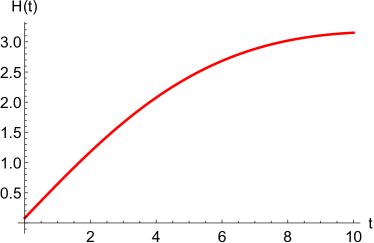
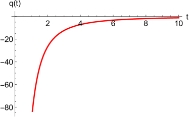
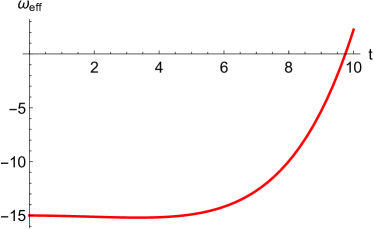
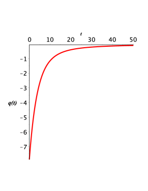
To understand cosmological nature of this exact solution, we study behavior of some important cosmological parameters graphically. We consider Hubble ($H$), deceleration ($q$) and effective equation of state ($w_{eff}$) parameters that measure rate of expansion and further characterize it into accelerating/decelerating phase of expansion. The negatively/positively evolving deceleration parameter discovers accelerating/decelerating phases of expanding cosmos while constant expansion appears for $q=0$. The effective EoS parameter classifies these accelerating/decelerating cosmic phases into distinct regimes as radiation ($\omega_{eff}=\frac{1}{3}$), matter ($\omega_{eff}=0$), quintessence ($-1<\omega\leq-1/3$) and phantom DE ($\omega<-1$) regimes. The mathematical forms of these standard parameters are given as

$$H=\frac{\dot{a}}{a},\quad q=-\frac{\dot{H}}{H^{2}}-1,\quad w_{eff}=\frac{p_{{}_{eff}}}{\rho_{{}_{eff}}}=\frac{p_{m}+p_{d}}{\rho_{m}+\rho_{d}}.$$

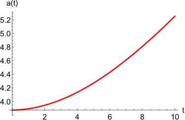
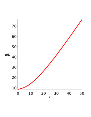
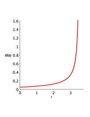
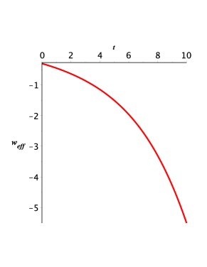
For graphical interpretation, we choose Mathemtica software with particular values of arbitrary constants that are mentioned in the caption of figures. The upper panel of figure 1 refers to accelerated expansion as both scale factor and Hubble parameter are positively increasing. In figure 1, the lower panel interprets evolution of deceleration (left) and effective EoS (right) parameters. Initially, both parameters correspond to accelerated expanding cosmos whereas a phase transition from accelerated to decelerated universe is observed with the passage of time. The deceleration parameter specifies constant state of expansion for $q=0$ while the effective EoS parameter identifies radiation-dominated phase of the universe.
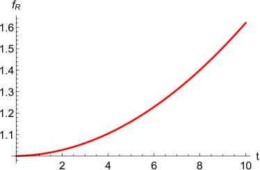
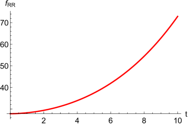
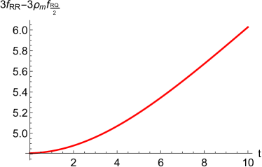
Refer to caption
Refer to caption
Refer to caption
Refer to caption
Figure 1: Plots of cosmological parameters versus cosmic time $t$ for $c_{2}=2$, $c_{3}=c_{4}=0.5$, $c_{9}=15$, $c_{11}=0.35$ and $c_{12}=0.05$.

Among gravitational theories, the $f(R)$ theory explores cosmic evolution as well as current expansion in the most remarkable manner. The formalism of this theory puts forward such spectacular models with positive/negative powers of curvature terms that unravel enigmatic mysteries behind early as well as late-time universe [26]. Besides this revolutionary incentive, the negative curvature terms may induce unfeasible behavior. This problem can be sorted out by imposing some constraints on higher-order curvature derivatives, i.e., $f_{R}>0,~{}f_{{}_{RR}}>0$ with $R>R_{0}$ ($R_{0}$ defines current scalar curvature) [27]. In non-minimally coupled gravitational theories, the appearance of an extra force also introduces instabilities against local perturbations [28]. These instabilities can be avoided by using Dolgov-Kawasaki instability criteria that demand positivity of higher-order curvature terms and matter variables [29]. In case of non-minimally coupled $f(R,T)$ theory, an additional constraint is suggested such as $1+f(R,T)_{T}>0$ [23]. For $f(R,T,Q)$ gravity, the Dolgov-Kawasaki instability analysis introduces two more conditions to achieve viable behavior given by

$$\frac{1+f_{{}_{T}}+1/2Rf_{{}_{Q}}}{f_{{}_{R}}-\mathcal{L}_{m}f_{{}_{Q}}}>0,\quad 3f_{{}_{RR}}+(1/2T-T^{00}f_{{}_{RQ}})\geq 0.$$ (33)

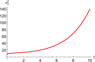
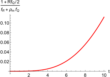
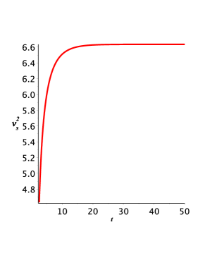
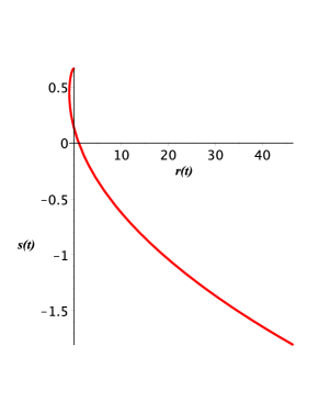
In order to determine stable/unstable nature of constructed models, the squared speed of sound comes up with simple criteria. The established model preserves its stable/unstable state against background perturbations for positively/negatively evolving squared speed of sound. The rβˆ’sπ‘Ÿπ‘ r-s parameters measure compatibility between constructed and well-known cosmological models for their particular values. A model is said to be consistent with $\Lambda$CDM, CDM models and Einstein universe if (r,sπ‘Ÿπ‘ r,s)=(1,0), (1,0) and (-$\infty$,$\infty$), respectively. For $s>0$ with $r<1$ and $s<0$ with $r>1$, the established model can be characterized as quintessence, phantom DE and Chaplygin gas models, respectively. The squared speed of sound and rβˆ’sπ‘Ÿπ‘ r-s parameters are given as

vs2=pd˙ρdΛ™,r=q+2​q2βˆ’qΛ™H,s=rβˆ’13​(qβˆ’12).formulae-sequencesuperscriptsubscript𝑣𝑠2Λ™subscript𝑝𝑑˙subscriptπœŒπ‘‘formulae-sequenceπ‘Ÿπ‘ž2superscriptπ‘ž2Λ™π‘žπ»π‘ π‘Ÿ13π‘ž12v_{s}^{2}=\frac{\dot{p_{d}}}{\dot{\rho_{d}}},\quad r=q+2q^{2}-\frac{\dot{q}}{H},\quad s=\frac{r-1}{3(q-\frac{1}{2})}.

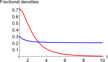
In the distinct regimes of expanding cosmos, the evaluation of fractional densities provides a better understanding of cosmological structure and matter distribution. According to Planck observational data, the fractional densities of flat cosmos are restricted to follow $\Omega_{m}+\Omega_{d}=1$, where $\Omega_{d}\simeq 0.6889$ and $\Omega_{m}\simeq 0.3111$ [30]. Mathematically, these fractional densities are given by

$$\Omega_{m}=\frac{\rho_{m}}{3m_{pl}^{2}H^{2}},\quad\Omega_{d}=\frac{\rho_{d}}{3m_{pl}^{2}H^{2}}.$$

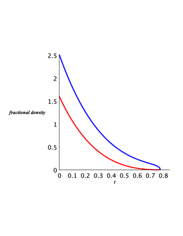
Figure 2 determines stable as well as viable $f(R,Q)$ model due to positive nature of the squared speed of sound and viability constraints. In figure 3 (left plot), the rβˆ’sπ‘Ÿπ‘ r-s parameters measure a consistency of established $f(R,Q)$ model with quintessence and phantom regions as $s>0$ when $r<1$. The right plot of figure 3 shows that initially, the fractional densities follow Planck observational constraint while this consistency is disturbed due to the dominance of $\Omega_{m}$ over $\Omega_{d}$ as time grows.

Refer to caption
Refer to caption
Refer to caption
Refer to caption
Refer to caption
Refer to caption
Figure 2: Plots of constructed $f(R,Q)$ model, squared speed of sound and viability conditions versus cosmic time $t$.
Refer to caption
Refer to caption
Figure 3: Plots of rβˆ’sπ‘Ÿπ‘ r-s parameters (left) and fractional densities (right) $\Omega_{m}$ (blue) and $\Omega_{d}$ (red) versus cosmic time $t$.

4 Noether Symmetries of $f(R,T)$ Model

In this case, we study the impact of non-minimal curvature-matter coupling in the background of pressureless fluid while the function $f$ is considered to be independent of the term $Q$. For these restrictions, we formulate all possible Noether symmetries and their associated conserved entities in the absence of boundary term ($\mathcal{B}=0$). For this purpose, the solutions to over determining system of non-linear equations (20)-(30) are given as

$\displaystyle\alpha$ $\displaystyle=$ $\displaystyle c_{6},\quad\beta=\frac{c_{1}c_{5}(c_{3}R-2c_{2}T^{2})+c_{1}^{2}c_{3}a^{3}R-2c_{1}c_{2}a^{3}T^{2}(c_{1}+T)}{c_{3}^{2}a(c_{5}+c_{1}a^{3}+a^{3}T)},\quad\psi=0,$
$\displaystyle\phi$ $\displaystyle=$ $\displaystyle\frac{c_{1}T}{c_{3}a},\quad\rho_{m}(a)=c_{1}+\frac{c_{5}}{a^{3}},\quad f(R,T)=(c_{3}\ln T+c_{4})R+c_{5}T^{2}+c_{7},$ (34)

where $c_{i}^{\prime}s~{}(i=1,2,...,7$) represent constants. In the case of simple Noether symmetry, we obtain $f(R,T)$ model that incorporates a direct non-minimal coupling between curvature and matter variables. For the sake of simplicity, we redefine constants as $c_{1}c_{3}c_{5}=d_{1},~{}c_{1}^{2}c_{3}=d_{2},~{}c_{1}c_{2}c_{5}=d_{3},~{}c_{1}^{2}c_{2}=d_{4},~{}c_{1}c_{2}=d_{5},~{}c_{1}/c_{3}=d_{6},~{}c_{3}^{2}c_{5}=d_{7},c_{1}c_{3}^{2}=d_{8}$ and $c_{3}^{2}=d_{9}$. For these constants, the group of Noether symmetries together with conserved integrals are

$\displaystyle Y_{1}$ $\displaystyle=$ $\displaystyle\partial_{{}_{a}},\quad I_{1}=12a\dot{a}f_{{}_{R}}+6a^{2}(\dot{R}f_{{}_{RR}}+\dot{T}f_{{}_{RQ}}),$ (35)
$\displaystyle Y_{2}$ $\displaystyle=$ $\displaystyle\frac{R}{d_{7}a+a^{4}(d_{8}+d_{9}T)}\partial_{{}_{R}},\quad I_{2}=\frac{6a^{2}\dot{a}f_{{}_{RR}}R}{d_{7}a+a^{4}(d_{8}+d_{9}T)},$
$\displaystyle Y_{3}$ $\displaystyle=$ $\displaystyle\frac{T}{a}\partial_{{}_{T}},\quad I_{3}=6a\dot{a}f_{{}_{RT}}T,$
$\displaystyle Y_{4}$ $\displaystyle=$ $\displaystyle\frac{a^{3}R}{d_{7}a+a^{4}(d_{8}+d_{9}T)}\partial_{{}_{R}},\quad I_{4}=\frac{6a^{5}\dot{a}f_{{}_{RR}}R}{d_{7}a+a^{4}(d_{8}+d_{9}T)},$
$\displaystyle Y_{5}$ $\displaystyle=$ $\displaystyle-\frac{2T^{2}}{d_{7}a+a^{4}(d_{8}+d_{9}T)}\partial_{{}_{R}},\quad I_{5}=-\frac{12a^{2}T^{2}\dot{a}f_{{}_{RR}}}{d_{7}a+a^{4}(d_{8}+d_{9}T)},$
$\displaystyle Y_{6}$ $\displaystyle=$ $\displaystyle-\frac{2a^{3}T^{2}}{d_{7}a+a^{4}(d_{8}+d_{9}T)}\partial_{{}_{R}},\quad I_{6}=-\frac{12a^{5}T^{2}f_{{}_{RR}}}{d_{7}a+a^{4}(d_{8}+d_{9}T)},$
$\displaystyle Y_{7}$ $\displaystyle=$ $\displaystyle-\frac{2a^{3}T^{3}}{d_{7}a+a^{4}(d_{8}+d_{9}T)}\partial_{{}_{R}},\quad I_{7}=-\frac{12a^{5}T^{3}f_{{}_{RR}}}{d_{7}a+a^{4}(d_{8}+d_{9}T)}.$

The correspondence of standard symmetries and conserved quantities cannot be established with the above set of seven symmetry generators and conserved integrals in the absence of boundary term. In order to study cosmological behavior of non-minimally coupled $f(R,T)$ model (34), we formulate exact solution of the scale factor from Eq.(35) given by

$\displaystyle a(t)$ $\displaystyle=$ $\displaystyle\frac{6I_{1}c_{5}}{t+c_{8}}\left[c_{3}Rootof(\mathcal{K})e^{-Rootof(\mathcal{K})}\right],$

where $\mathcal{K}=I_{1}^{3}(t+c_{8})e^{2\mathcal{Z}}-216c_{5}^{2}(c_{3}\mathcal{Z}+c_{4})^{3}$ and $c_{8}$ indicates integration constant whereas $\mathcal{Z}$ denotes global variable.

Refer to caption
Refer to caption
Refer to caption
Refer to caption
Figure 4: Plots of cosmological parameters versus cosmic time $t$ for $c_{1}=-0.01$, $I_{1}=c_{4}=10$, $c_{5}=c_{8}=0.01$, $c_{3}=1.25$, $c_{7}=2.5$ and $c_{12}=0.05$.
Refer to caption
Refer to caption
Refer to caption
Refer to caption
Figure 5: Plots of constructed $f(R,T)$ model, squared speed of sound and viability conditions versus cosmic time $t$.
Refer to caption
Refer to caption
Figure 6: Plots of rβˆ’sπ‘Ÿπ‘ r-s parameters (left) and fractional densities (right) $\Omega_{m}$ (blue) and $\Omega_{d}$ (red) versus cosmic time $t$.

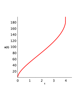
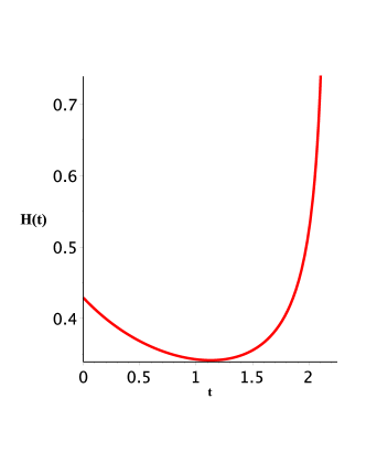
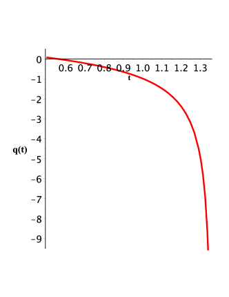
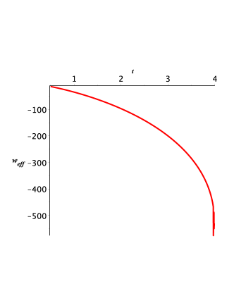
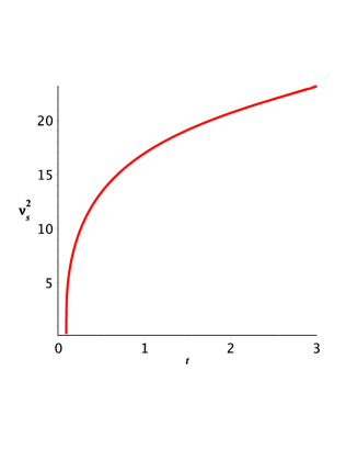
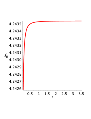
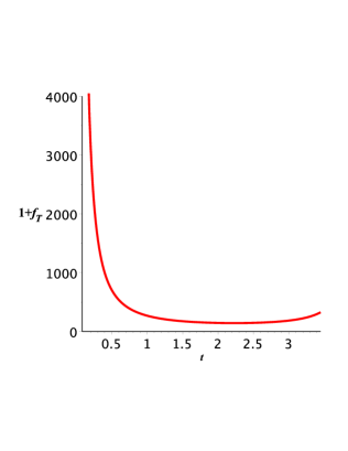
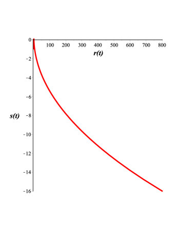
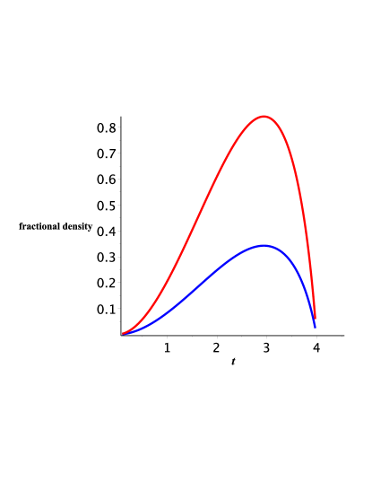
Figure 4 develops cosmological understanding for exact solution of scale factor through Hubble, deceleration and effective EoS parameters. The graphical representation of these parameters ensures accelerated cosmic expansion while EoS further characterizes a smooth transition from quintessence to phantom DE era. Figure 5 measures the evolution as well as realistic nature of non-minimally coupled $f(R,T)$ model via squared speed of sound and viability constraints. It is interesting to mention here that the established model is stable and viable in the background of accelerated expanding cosmos. In Figure 6, the model is found to be consistent with Chaplygin gas model as $r>1$ and $s<0$ (left plot) while the dominance of DE energy density over matter energy density shows consistency with recent observational data (right plot).

5 Noether Symmetries of $f(T,Q)$ Model

In this section, the source of non-minimal interactions is considered to be trace of energy-momentum tensor, contracted Ricci and energy-momentum tensors while the generic function is considered to be free from curvature invariant. To investigate the effect of these interactions, we solve the system (20)-(30) to determine possible symmetries and corresponding conservation laws for $f(T,Q)$ model. In this regard, we consider $\phi(a,R,T,Q),_{R}=\psi(a,R,T,Q)_{R}=0$ and obtain the resulting solution as follows

$\displaystyle\alpha$ $\displaystyle=$ $\displaystyle c_{1},\quad\beta=0,\quad\phi=-\frac{c_{6}Q}{c_{3}a^{2}(c_{7}+T)},\quad\psi=\frac{c_{8}}{c_{9}a^{2}},$
$\displaystyle f(T,Q)$ $\displaystyle=$ $\displaystyle c_{3}T+c_{4}Q+c_{5},\quad\rho_{m}(a)=c_{1}a+c_{2}.$ (36)

The formulated $f(T,Q)$ model admits implicit non-minimal interactions while the generators and respective conserved integrals of simple Noether symmetry turn out to be

$\displaystyle Y_{1}$ $\displaystyle=$ $\displaystyle\partial_{{}_{a}},\quad I_{1}=-6a\dot{a}f_{{}_{Q}}(2\rho_{m}+a\rho_{m}^{\prime})+3a^{2}\rho_{m}(\dot{T}f_{{}_{TQ}}+\dot{Q}f_{{}_{QQ}}),$ (37)
$\displaystyle Y_{2}$ $\displaystyle=$ $\displaystyle-\frac{Q}{a^{2}c_{3}(c_{7}+T)}\partial_{{}_{T}},\quad I_{2}=\frac{3\dot{a}\rho_{m}Qf_{{}_{TQ}}}{c_{3}(c_{7}+T)},$
$\displaystyle Y_{3}$ $\displaystyle=$ $\displaystyle\frac{1}{a^{2}c_{9}}\partial_{{}_{Q}},\quad I_{3}=-\frac{3\dot{a}\rho_{m}f_{{}_{QQ}}}{c_{9}}.$

The symmetry generator $Y_{1}$ defines scaling symmetry and correspondingly, $I_{1}$ refers to conservation of linear-momentum. Besides the conserved linear-momentum, the first Noether integral (37) also helps to determine exact solution for $I_{1}=0$ given as

$\displaystyle a(t)$ $\displaystyle=$ $\displaystyle\left[-LambertW\left(-\frac{e^{\frac{2c_{1}c_{10}+2tc_{1}-c_{2}}{c_{2}}}}{c_{2}}\right)+\frac{2c_{1}c_{10}+2tc_{1}-c_{2}}{c_{2}}\right]$
$\displaystyle\times$ $\displaystyle\frac{2c_{1}c_{10}+2tc_{1}-c_{2}}{c_{1}}.$

In Figure 7, the scale factor as well as cosmological parameters measure an accelerated expansion that favors a smooth transition from quintessence to phantom DE phase. The positively evolving minimally coupled $f(T,Q)$ model is found to be unstable at early stage as $v_{s}^{2}<0$ while the model attains stability as time passes (Figure 8, upper panel). It is interesting to mention here that the established model satisfies all viability constraints for $c_{3},~{}c_{4}\geq 0$ whereas rβˆ’sπ‘Ÿπ‘ r-s parameters specify correspondence with Chaplygin gas model (Figure 8, lower panel). Figure 9 indicates that at $t=0.34$, the fractional densities relative to matter and DE are found to be compatible with Planck’s observational data.

Refer to caption
Refer to caption
Refer to caption
Refer to caption
Figure 7: Plots of scale factor, Hubble, deceleration and effective EoS parameters versus cosmic time $t$ for $c_{1}=-0.2$, $c_{2}=-1.5$, $c_{3}=2$, $c_{4}=1.05$, $I_{2}=0$, $c_{5}=1$ and $c_{10}=-2$.
Refer to caption
Refer to caption
Refer to caption
Figure 8: Plots of $f(T,Q)$ (upper left), squared speed of sound (upper right), viability condition (lower left) and rβˆ’sπ‘Ÿπ‘ r-s parameters (lower right) versus cosmic time $t$.
Refer to caption
Figure 9: Plots of fractional densities (right) $\Omega_{m}$ (blue) and $\Omega_{d}$ (red) versus cosmic time $t$.

6 Noether Symmetry of $f(R,T,Q)$ Model

This case determines the existence of Noether point symmetries and corresponding conserved entities in the presence of non-minimal scalar curvature and matter variables. In order to solve the system of non-linear equations (20)-(30) for Noether symmetry, we consider $\alpha=F_{1}(a)F_{2}(R)F_{3}(T)F_{4}(Q)$ and $\beta=d_{1}$, which gives

$\displaystyle\alpha=\frac{c_{6}(Rc_{1}+c_{2})(Tc_{4}+c_{5})(c_{3}+2a^{\frac{2}{3}}Q)}{c_{3}a^{\frac{7}{6}}},\quad\beta=c_{8},\quad\phi=-\frac{2a^{\frac{2}{3}}(Tc_{4}+_{5})\psi}{c_{4}},$
$\displaystyle\psi=-\frac{6c_{6}(Tc_{4}+c_{5})(Rc_{1}+c_{2})\Sigma}{a^{\frac{5}{2}}c_{3}c_{4}(c_{1}a^{\frac{1}{3}}+aT)},\quad\rho_{m}(a)=\frac{c_{6}}{a^{\frac{2}{3}}},$
$\displaystyle f(R,T,Q)=c_{4}T\exp[Rc_{1}+2a^{\frac{2}{3}}Q+c_{3}].$ (38)

Here, the formulated exponential $f(R,T,Q)$ model admits strong non-minimal interactions between scalar curvature and matter variables whereas $\Sigma$ is defined as

$\displaystyle\Sigma$ $\displaystyle=$ $\displaystyle\frac{(R(Tc_{4}+c_{5})c_{1}+Tc_{3}c_{4}+c_{5}(c_{3}-1))Qa^{\frac{4}{3}}}{2}+Q^{2}a^{2}(Tc_{4}+c_{5})+\frac{7c_{1}c_{3}c_{4}}{36}$
$\displaystyle+$ $\displaystyle\left(\left(\left(\frac{RTc_{3}}{4}+\frac{7Q}{8}\right)c_{4}+\frac{Rc_{3}c_{5}}{4}\right)c_{1}-\frac{c_{3}c_{5}}{4}\right)a^{\frac{2}{3}}.$

The arbitrary constants are denoted by $c_{i}~{}(i=1,2,...,6$) while the resulting solution satisfies over-determining system for $c_{2}=c_{5}=0$. For the sake of simplicity, we redefine a few constants such as $c_{1}c_{4}c_{6}=d_{2},~{}\frac{c_{1}c_{4}c_{6}}{c_{3}}=d_{3},~{}c_{1}^{2}c_{4}c_{6}=d_{4}$ and $\frac{c_{1}^{2}c_{4}c_{6}}{c_{3}}=d_{5}$. In this case, we find the set of symmetry generators and respective conserved entities as follows

$\displaystyle Y_{1}$ $\displaystyle=$ $\displaystyle\partial_{{}_{R}},\quad I_{1}=6a^{2}\dot{a}f_{{}_{RR}}-6a^{2}\dot{a}\rho_{m}f_{{}_{RQ}},$
$\displaystyle Y_{2}$ $\displaystyle=$ $\displaystyle\frac{2RTQ}{a^{\frac{1}{2}}}\partial_{{}_{a}}+\frac{6RT^{2}Q^{2}}{c_{1}a^{\frac{1}{3}}+aT}\left(2a^{\frac{1}{6}}T\partial_{{}_{T}}-\frac{1}{\sqrt{a}}\partial_{{}_{Q}}\right),$
$\displaystyle I_{2}$ $\displaystyle=$ $\displaystyle\frac{2RTQ}{\sqrt{a}}\left(12a\dot{a}f_{{}_{R}}+6a^{2}(\dot{R}f_{{}_{RR}}+\dot{T}f_{{}_{RT}}+\dot{Q}f_{{}_{RQ}})-6a\dot{a}f_{{}_{Q}}(2\rho_{m}+a\rho_{m}^{\prime})\right.$
$\displaystyle-$ $\displaystyle\left.3a^{2}\rho_{m}(\dot{R}f_{{}_{RQ}}+\dot{T}f_{{}_{TQ}}+\dot{Q}f_{{}_{QQ}})\right)+\frac{12a^{2}RT^{3}Q^{2}}{a^{\frac{11}{6}}(c_{1}a^{\frac{1}{3}}+aT)}(6a^{2}\dot{a}f_{{}_{RT}}-3a^{2}\dot{a}\rho_{m}f_{{}_{TQ}})$
$\displaystyle-$ $\displaystyle\frac{6a^{2}RT^{2}Q^{2}}{a^{\frac{5}{2}}(c_{1}a^{\frac{1}{3}}+aT)}(6a^{2}\dot{a}f_{{}_{RQ}}-3a^{2}\dot{a}\rho_{m}f_{{}_{QQ}}),$
$\displaystyle Y_{3}$ $\displaystyle=$ $\displaystyle\frac{RT}{a^{\frac{7}{6}}}\partial_{{}_{a}}+\frac{3RT^{2}Q}{c_{1}a^{\frac{1}{3}}+aT}\left(\frac{2T}{\sqrt{a}}\partial_{{}_{T}}-\frac{1}{a^{\frac{1}{3}}}\partial_{{}_{Q}}\right),$
$\displaystyle I_{3}$ $\displaystyle=$ $\displaystyle\frac{RT}{a^{\frac{7}{6}}}\left(12a\dot{a}f_{{}_{R}}+6a^{2}(\dot{R}f_{{}_{RR}}+\dot{T}f_{{}_{RT}}+\dot{Q}f_{{}_{RQ}})-6a\dot{a}f_{{}_{Q}}(2\rho_{m}+a\rho_{m}^{\prime})\right.$
$\displaystyle-$ $\displaystyle\left.3a^{2}\rho_{m}(\dot{R}f_{{}_{RQ}}+\dot{T}f_{{}_{TQ}}+\dot{Q}f_{{}_{QQ}})\right)+\frac{6RT^{3}Q}{a^{\frac{1}{2}}(c_{1}a^{\frac{1}{3}}+aT)}(6a^{2}\dot{a}f_{{}_{RT}}-3a^{2}\dot{a}\rho_{m}f_{{}_{TQ}})$
$\displaystyle-$ $\displaystyle\frac{3RT^{2}Q}{a(c_{1}a^{\frac{1}{3}}+aT)}(6a^{2}\dot{a}f_{{}_{RQ}}-3a^{2}\dot{a}\rho_{m}f_{{}_{QQ}}),$
$\displaystyle Y_{4}$ $\displaystyle=$ $\displaystyle\left(\frac{7+9a^{\frac{2}{3}}RT}{c_{1}a^{\frac{1}{3}}+aT}\right)\left[\frac{RT^{2}}{3a^{\frac{11}{6}}}\partial_{{}_{T}}-\frac{RT}{6a^{\frac{5}{2}}}\partial_{{}_{Q}}\right],\quad I_{4}=\frac{RT^{2}(7+9a^{\frac{2}{3}}RT)}{3a^{\frac{11}{6}}(c_{1}a^{\frac{1}{3}}+aT)}$
$\displaystyle\times$ $\displaystyle(6a^{2}\dot{a}f_{{}_{RT}}-3a^{2}\dot{a}\rho_{m}f_{{}_{TQ}})-\frac{RT(7+9a^{\frac{2}{3}}RT)}{6a^{\frac{5}{2}}(c_{1}a^{\frac{1}{3}}+aT)}(6a^{2}\dot{a}f_{{}_{RQ}}-3a^{2}\dot{a}\rho_{m}f_{{}_{QQ}}),$
$\displaystyle Y_{5}$ $\displaystyle=$ $\displaystyle\left(\frac{14a^{\frac{2}{3}}Q+18a^{\frac{4}{3}}RT}{c_{1}a^{\frac{1}{3}}+aT}\right)\left[\frac{RT^{2}}{3a^{\frac{11}{6}}}\partial_{{}_{T}}-\frac{RT}{6a^{\frac{5}{2}}}\partial_{{}_{Q}}\right],\quad I_{5}=\frac{2RT^{2}Qa^{\frac{2}{3}}(7+9a^{2}RT)}{3a^{\frac{11}{6}}(c_{1}a^{\frac{1}{3}}+aT)}$
$\displaystyle\times$ $\displaystyle(6a^{2}\dot{a}f_{{}_{RT}}-3a^{2}\dot{a}\rho_{m}f_{{}_{TQ}})-\frac{a^{\frac{2}{3}}RTQ(7+9a^{\frac{2}{3}}RT)}{3a^{\frac{5}{2}}(c_{1}a^{\frac{1}{3}}+aT)}(6a^{2}\dot{a}f_{{}_{RQ}}-3a^{2}\dot{a}\rho_{m}f_{{}_{QQ}}).$

The symmetry generator $Y_{1}$ identifies scaling symmetry whereas associated conserved integral $I_{1}$ defines conservation of linear momentum. In the present case, it is too difficult to evaluate explicit form of the scale factor for the established exponential $f(R,T,Q)$ model.

7 Final Remarks

The non-minimally coupled gravitational theories put forward fascinating approaches to explore evolutionary phases of the cosmos from its origin to the current state. This work determines exact solution of flat and isotropic cosmos filled with dust distribution via Noether symmetry scheme in $f(R,T,Q)$ theory. Following this approach, a system with non-zero boundary term ($\mathcal{B}\neq 0$) preserves Noether gauge symmetry while dynamical system with zero boundary term ($\mathcal{B}=0$) recovers simple Noether point symmetry. These symmetries are categorized into translational and spatial symmetries identifying corresponding conservation laws, i.e., energy and linear/angular momentum conservation, respectively.

In order to discuss the impact of weak or strong interactions between curvature invariant and matter variables on geodesic/non-geodesic test particles, we have considered different non-minimally coupled models such as $f(R,Q)$, $f(R,T)$ and $f(T,Q)$ models. For each choice and general $f(R,T,Q)$ model, we have found scaling symmetry along conservation of linear momentum for $f(R,Q),~{}f(T,Q)$ and $f(R,T,Q)$ models. For $f(R,T)$ model, the system of over-determining equations fail to produce scaling symmetry and relative conservation law. For each considered model, the explicit forms of energy density and generic function are calculated that yield exact solutions for scale factor whereas for general $f(R,T,Q)$ model, the formulation of exact solution is not possible. We have studied the cosmological nature of these solutions via graphical analysis of some standard parameters, i.e., Hubble, deceleration and effective EoS parameters. According to Planck 2018 constraints, the suggested values of $H$ at $68\%CL$ are given by [30]

$\displaystyle H_{0}$ $\displaystyle=$ $\displaystyle 67.27\pm 0.60\quad\text{(TT+TE+EE+low E)},$
$\displaystyle H_{0}$ $\displaystyle=$ $\displaystyle 67.36\pm 0.54\quad\text{(TT+TE+EE+low E+lensing)},$
$\displaystyle H_{0}$ $\displaystyle=$ $\displaystyle 67.66\pm 0.42\quad\text{(TT+TE+EE+low E+lensing+BAO)}.$

Furthermore, we have investigated the existence of physically viable and stable state of new $f(R,Q),~{}f(R,T),~{}f(T,Q)$ and $f(R,T,Q)$ models through the squared speed of sound and well-known Dolgov-Kawasaki viability conditions. The matter distribution is also analyzed using fractional densities relative to pressureless fluid and DE. The observational constraints on $\Omega_{m}$ and $\Omega_{d}$ with $68\%$CL are given as [30]

$\displaystyle\Omega_{m}=0.3166\pm 0.0084,\quad\Omega_{d}=0.7116\pm 0.0084,$
$\displaystyle\text{(TT+TE+EE+low E)},$
$\displaystyle\Omega_{m}=0.3158\pm 0.0073,\quad\Omega_{d}=0.6847\pm 0.0073,$
$\displaystyle\text{(TT+TE+EE+low E+lensing)},$
$\displaystyle\Omega_{m}=0.3111\pm 0.0056,\quad\Omega_{d}=0.68889\pm 0.0056,$
$\displaystyle\text{(TT+TE+EE+low E+lensing+BAO)}.$

The consistency of above mentioned parameters is checked against recent observational data of Planck 2018. The results are summarized as follows.

  • β€’

    f​(R,Q)𝑓𝑅𝑄f(R,Q) Model

In the absence of boundary term, the cosmological parameters identify a transition from accelerated to decelerated expansion while the stable as well as viable $f(R,Q)$ model describes phantom and quintessence regions. The fractional densities meet with Planck limitations whereas the consistency disturbs as time passes due to the dominance of matter fractional density. Zubair et al. [31] investigated cosmic evolution using particular $f(R,Q)$ model and power-law Hubble parameter without using Noether Symmetry approach. They constructed model constraints that refer to $\Lambda$CDM limit and explain current accelerated expansion.

  • β€’

    f​(R,T)𝑓𝑅𝑇f(R,T) Model

For this choice of model, the cosmological analysis characterizes a smooth exit from quintessence to phantom DE era. The stable and viable non-minimally coupled $f(R,T)$ model is found to be consistent with Chaplygin gas model. The graphical evaluation of fractional densities supports accelerated expansion of the universe. Momeni et al. [19] used simple Noether symmetry technique to evaluate symmetry generators and conserved integral in $f(R,T)$ theory. They considered minimally interacting $f(R,T)$ model and determined exact solution corresponding to decelerated expansion of the cosmos whereas we have found non-minimal $f(R,T)$ model specifying accelerated cosmic expansion. In this regard, it is interesting to mention that current accelerated expansion can successfully be discussed in the presence of non-minimal interactions of scalar curvature and matter contents.

  • β€’

    f​(T,Q)𝑓𝑇𝑄f(T,Q) Model

The graphical study of cosmological parameters leads to accelerated expansion of the universe for evaluated Noether point symmetries. The minimally coupled viable $f(T,Q)$ model is found to be consistent with Chaplygin gas model whereas the model becomes unstable initially but recovers a stable state as time grows. The fractional densities are consistent with accelerated expanding cosmos for zero boundary term.

  • β€’

    f​(R,T,Q)𝑓𝑅𝑇𝑄f(R,T,Q) Model

For the generalized non-minimally coupled model, we have found an explicit form of energy density and exponential $f(R,T,Q)$ model. In this case, we have determined five symmetry generators out of which only one identifies scaling symmetry with linear conservation of momentum. Due to strong non-minimal interactions between curvature-matter variables, it is not possible to measure cosmological solution.

Sharif and Gul [32] examined some physically viable anisotropic solutions through the Noether symmetry technique in $f(R,T^{2})$ theory. They considered a minimally coupled $f(R,T^{2})$ model to determine exact solutions and examined the behavior of solutions via some cosmological parameters. For Bianchi type III model, the graphical behavior of cosmological parameters represent accelerated expansion whereas analysis of fractional densities does not preserve this consistency for the same model. In case of Kantowski-Sachs model, the parameters identify decelerated expansion while DE fractional density dominates matter fractional density. In the present study, we have formulated non-minimally coupled isotropic exact solutions. For non-minimal geodesic $f(R,Q)$ model, the cosmological parameters identify a transition from accelerated to decelerated expansion whereas the fractional densities analysis shows dominance of DE initially and this dominance disturbs as time passes due to increasing amount of matter fractional density. For constructed non-geodesic $f(R,T)$ model, the parameters characterize a smooth exit from quintessence to phantom DE era while fractional densities support accelerated expansion of the universe. In case of minimal non-geodesic $f(T,Q)$ solution, the study of cosmological parameters and fractional densities lead to accelerated expansion of the universe. Thus, it is worth notifying that the analysis of present cosmological solutions and fractional densities are compatible with each other.

Finally, We have found scaling symmetry generator and linear momentum conservation for each case except for $f(R,T)$ model, where symmetries and respective conservation laws do not correspond to any standard symmetry or conserved entity. The new non-minimally coupled models are found to be stable and viable in the background of pressureless fluid. These models also preserve compatibility with Chaplygin gas model, quintessence and phantom regions. It is interesting to conclude that the isotropic cosmological solutions interpret accelerated cosmic expansion whenever generic function involves non-minimal coupling. It would be interesting to explore the impact of non-minimal curvature-matter coupling in the background of anisotropic universe models. Using Noether symmetry approach, the study of cosmological configurations like black hole and wormhole would be much fascinating.

Data Availability Statement: No new data were created or analyzed in this study.

References

  • [1] Shankaranarayanan, S. and Joseph P.J.: Gen. Relativ. Gravit.54(2022)44.
  • [2] Sotiriou, T.P. and Faraoni, V.: Rev. Mod. Phys. 82(2010)451; Felice, A.D. and Tsujikawa, S.: Living Rev. Rel. 13(2010)3; Nojiri, S. and Odintsov, S.D.: Phys. Rept. 505(2011)59; Bamba, K. et al.: Astrophys. Space Sci. 342(2012)155.
  • [3] Bertolami, O. et al.: Phys. Rev. D 75(2007)104016.
  • [4] Harko, T. et al.: Phys. Rev. D 84(2011)024020.
  • [5] Bertolami, O. and Sequeira, M.C.: Phys. Rev. D 79(2009)104010; Bertolami, O. and Paramos, J.: J. Cosmol. Astropart. Phys. 03(2010)009; Bertolami, O., Frazao, P. and Paramos, J.: Phys. Rev. D 81(2010)104046; Bertolami, O., Frazao, P. and Paramos, J.: Phys. Rev. D 83(2011)044010.
  • [6] Sharif, M. and Zubair, M.: J. Cosmol. Astropart. Phys. 03(2012)028; J. Exp. Theor. Phys. 117(2013)248; J. Phys. Soc. Jpn. 82(2013)014002; ibid. 82(2013)064001; Astrophys. Space Sci. 349(2014)52; Gen. Relativ. Gravit. 46(2014)1723.
  • [7] Sharif, M. and Zubair, M.: J. Cosmol. Astropart. Phys. 11(2013)042; J. High Energy Phys. 12(2013)079; Yousaf, Z. et al.: Eur. Phys. J. A 54(2018)122; Bhatti, M.Z. et al.: J. Cosmol. Astropart. Phys. 09(2019)011; Yousaf, Z., Bhatti, M.Z. and Naseer, T.: Eur. Phys. J. Plus 135(2020)323.
  • [8] Sebastiani, L. and Zerbini, S.: Eur. Phys. J. C 71(2011)1591.
  • [9] Maharaj, S.D. et al.: Mod. Phys. Lett. A 32(2017)1750164.
  • [10] Sharif, M. and Zubair, M.: Astrophys. Space Sci. 349(2014)457.
  • [11] Harko, T. and Lake, M.J.: Eur. Phys. J. C 75(2015)60.
  • [12] Shamir, M.F.: Eur. Phys. J. C 75(2015)354.
  • [13] Zahid, M., Khan, S. U. and Ren, J.: Chin. J. Phys. 72(2021)575; Zahid, M., Rayimbaev, J., Khan, S. U., Ren, J., Ahmedov, S. and Ibragimov, I.: Eur. Phys. J. C 82(2022)494; Zahid, M., Khan, S. U., Ren, J. and Rayimbaev, J.: Int. J. Mod. Phys. D 31(2022)2250058.
  • [14] Capozziello, S., Stabile, A. and Troisi, A.: Class. Quantum Grav. 24(2007)2153.
  • [15] Hussain, I., Jamil, M. and Mahomed, F.M.: Astrophys. Space Sci. 337(2012)373.
  • [16] Shamir, M.F., Jhangeer, A. and Bhatti, A.A.: Chin. Phys. Lett. 29(2012)080402.
  • [17] Oz, I.B. and Bamba, K.: Eur. Phys. J. C 82(2022)349.
  • [18] Atazadeh, K. and Darabi, F.: Eur. Phys. J. C 72(2012)2016.
  • [19] Momeni, D., Myrzakulov, R. and Gudekli, E.: Int. J. Geom. Methods Mod. Phys. 12(2015)1550101.
  • [20] Sharif, M. and Fatima, I.: J. Exp. Theor. Phys. 122(2016)104; Sharif, M. and Nawazish, I.: J. Exp. Theor. Phys. 120(2014)49; Eur. Phys. J. C 77(2017)198; Mod. Phys. Lett. A 32(2017)1750136; Gen. Relativ. Gravit.49(2017)76.
  • [21] Sharif, M. and Nawazish, I.: Ann. Phys. 389(2018)283; ibid. 400(2019)37; Sharif, M., Nawazish, I. and Hussain, S.: Eur. Phys. J. C 80(2020)783.
  • [22] Bahamonde, S., Bamba, K. and Camci, U.: J. Cosmol. Astropart. Phys. 02(2019)016; Shamir, M.F., Malik, A. and Ahmad, M.: Theoret. Math. Phys. 205(2020)1692; Malik, A. Shamir, M.F. and Hussain, I.: Int. J. Geom. Methods Mod. Phys. 17(2020) 2050163.
  • [23] Odintsov, S.D. and Saez-Gomez, D.: Phys. Lett. B 725(2013)437.
  • [24] Sotiriou, T.P. and Faraoni, V.: Class. Quantum Grav. 25(2008)205002; Bertolami, O. and Paramo, J.: Class. Quantum Grav. 25(2008)245017.
  • [25] Basilakos, S., Tsamparlis, M. and Paliathanasis, A.: Phys. Rev. D 83(2011)103512; ibid. 84(2011)123514; Capozziello, S., De Laurentis, M. and Odintsov, S.D.: Eur. Phys. J. C 72(2012)1434; Basilakos, S. et al.: Phys. Rev. D 88(2013)103526; Paliathanasis, A. et al.: Phys. Rev. D 89(2014)063532.
  • [26] Capozziello, S.: Int. J. Mod. Phys. D 11(2002)483; Nojiri, S. and Odintsov, S.D.: Gen. Relativ. Gravit. 36(2004)1765.
  • [27] Dolgov, A.D. and Kawasaki, M.: Phys. Lett. B 573(2003)1; Faraoni, V.: Phys. Rev. D 74(2006)104017.
  • [28] Haghani, Z. et al.: Phys. Rev. D 88(2013)044023.
  • [29] Harko,T. and Lobo, F.S.N.: Int. J. Mod. Phys. D 29(2020)2030008.
  • [30] Aghanim, N. et al.: Astron. Astrophys. A 6(2020)641.
  • [31] Zubair, M., Zeeshan, M. and Waheed, S.: Mod. Phys. Lett. A 34(2019)1950253.
  • [32] Sharif, M. and Gul, Z.M.: J. Exp. Theor. Phys. 136(2023)436.