Greedy Newton: Newton’s Method with Exact Line Search

Abstract

A defining characteristic of Newton’s method is local superlinear convergence within a neighbourhood of a strict local minimum. However, outside this neighborhood Newton’s method can converge slowly or even diverge. A common approach to dealing with non-convergence is using a step size that is set by an Armijo backtracking line search. With suitable initialization the line-search preserves local superlinear convergence, but may give sub-optimal progress when not near a solution. In this work we consider Newton’s method under an exact line search, which we call “greedy Newton” (GN). We show that this leads to an improved global convergence rate, while retaining a local superlinear convergence rate. We empirically show that GN may work better than backtracking Newton by allowing significantly larger step sizes.

1 Introduction

For minimizing a twice-differentiable function $f:\mathbb{R}^{n}\rightarrow\mathbb{R}$, the pure Newton iteration $x_{k+1}^{N}$ starting from some vector $x_{k}$ is given by

$$x_{k+1}^{N}=x_{k}-\nabla^{2}f(x_{k})^{-1}\nabla f(x_{k}).$$ (1)

This method dates back to work by Newton and Raphson in the 1600s for finding roots of polynomials [4]. Since then, the method has evolved to work in a variety of settings. In optimization, Newton’s method is a powerful tool for minimizing non-linear objectives mainly due to its remarkable property of superlinear (quadratic) convergence in a neighborhood of a strict local minimum (under appropriate conditions) [see 2, Section 9.5].

However, Newton’s method also has known weaknesses. For example, the method is not guaranteed to converge in general or even decrease $f$. One of the standard fixes to the non-convergence is to introduce a step size $\alpha_{k}$,

$$x_{k+1}=x_{k}-\alpha_{k}\nabla^{2}f(x_{k})^{-1}\nabla f(x_{k}).$$ (2)

The step size is typically set by first considering $\alpha_{k}=1$ and dividing the step size by a fixed constant (“backtracking”) until the Armijo condition is satisfied [2, Section 9.5]. Provided that we eventually get close enough to a strict local minimum, Armijo backtracking preserves the superlinear convergence of the pure Newton method. Many variations of Newton’s method exist such as modifications for cases where the $\nabla^{2}f(x_{k})$ is not invertible. Other variations include those based on trust-region methods instead of line searches [see 13], but the superlinear convergence proofs in the literature that we are aware of for eq:GN_update assume we first test $\alpha_{k}=1$ and accept this step size if it satisfies a variant of the Armijo condition.

While $\alpha_{k}=1$ becomes asymptotically optimal in the neighbourhood of a strict local minimizer, it may not be the optimal step size even when close to a minimizer. Further, when far away from a local minimizer using $\alpha_{k}=1$ or the smaller values obtained by backtracking may converge slowly. This paper instead investigates Newton’s method where the step size is set to minimize the function value,

$$\alpha_{k}\in\mathop{\rm arg\,min}_{\alpha}f(x_{k}-\alpha\nabla^{2}f(x_{k})^{-1}\nabla f(x_{k}))$$ (3)

We call using this exact line search within Newton’s method the “greedy Newton” (GN) method. We first address two mis-conceptions the reader may have about this method:

• It typically does not significantly increase the cost of Newton’s method to find a local minimizer of eq:newton_exactLS. For most problems just computing the Hessian is $n$-times more expensive than evaluating the function or directional derivatives. Thus, you can evaluate the objective in eq:newton_exactLS and its derivative several times without changing the overall cost of the method. As an example, consider logistic regression with $m$ training examples $\{a_{i},b_{i}\}$ with dense features $a_{i}\in\mathbb{R}^{n}$ and binary labels $b_{i}\in\{-1,1\}$,

  $$f(x)=\sum_{i=1}^{m}\log(1+\exp(-b_{i}x^{T}a_{i})).$$ (4)

  The cost of computing the Hessian for this problem is $O(mn^{2})$, but the cost of evaluating $f$ or a directional derivative of it is only $O(mn)$. With bisection we can solve the one-dimensional problem eq:newton_exactLS to $\epsilon$ accuracy over a bounded domain in $O(\log(1/\epsilon))$ iterations, so the cost of a naive black-box numerical method is only $O(mn\log(1/\epsilon))$.

  Further, if we exploit the linear composition structure of  eq:logreg the cost of bisection can be reduced to $O(mn+m\log(1/\epsilon))$. It is also possible to use faster one-dimensional minimizers like the secant method. Indeed, low-cost line searches are possible for a wide variety of problems including linear models, matrix factorization models, and certain neural networks [9; 10; 17; 18; 15].

• The exact line search can yield a significantly smaller function value than Armijo backtracking. The optimal step size eq:newton_exactLS may be significantly larger than the maximum step size of $1$ considered in standard implementations. While we could backtrack from a step size larger than $1$, the Armijo condition itself can exclude the optimal step size. Indeed, for non-quadratic functions the maximum step size allowed by the Armijo condition can be arbitrarily worse than the optimal step size.

By modifying standard arguments for the convergence of Newton’s method, we show:

1. For strongly-convex functions with a Lipschitz-continuous gradient, GN slightly improves the global convergence rate compared to Armijo backtracking (Section 2.1).

2. Under the additional assumption that the Hessian is Lipschitz-continuous, superlinear convergence is achieved by any method that decreases the function value by at least as much as the pure Newton iteration eq:newton_update (Section 2.2).

3. Local convergence rate of Newton’s method with non-unit step sizes (Section 2.3).

4. Hybrid Newton-gradient methods that further improve the global convergence rate of Netwon’s method (Section 2.4).

We are not aware of the superlinear convergence of GN appearing previously in the literature, although recent work bounds the GN step size for self-concordant functions [6] and various progress measures give superlinear convergence for solving non-linear equations [3]. In Section 3 we xxperiment with the GN method for logistic regression. Our findings suggest that GN consistently works better than using Armijo backtracking, and substantially better for certain problems where the optimal step sizes can be much larger than 1.

2 Convergence of Greedy Newton Methods

All our results assume that $f$ is twice-differentiable and that the eigenvalues of the Hessian $\nabla^{2}f$ are bounded between positive constants $\mu$ and $L$ for all $x$,

$$\mu I\preceq\nabla^{2}f(x)\preceq LI.$$ (5)

These assumptions are equivalent to assuming that $\nabla f$ is $L$-Lipschitz continuous and that $f$ is $\mu$-strongly convex. We note that without these assumptions GN may not converge [8; 7], but various Hessian modifications guarantee convergence [see 13, Section 3.4]. The local superlinear convergence results also require that the Hessian is $M$-Lipschitz continuous,

$$\|\nabla^{2}f(x)-\nabla^{2}f(y)\|\leq M\|x-y\|,$$ (6)

where the matrix norm $\|\cdot\|$ on the left is the spectral norm. We give proofs of the results in this section in Appendix A.

2.1 Global Convergence of Greedy Newton

We first give a global rate of convergence for the GN method.

Proposition 2.1.

Let a twice-differentiable $f$ be $\mu$-strongly convex with an $L$-Lipschitz continuous gradient eq:Lmu. Then the iterations of Newton’s method eq:GN_update with the greedy step size eq:newton_exactLS satisfy

$$f(x_{k})-f(x_{*})\leq\left(1-\frac{\mu^{2}}{L^{2}}\right)^{k}[f(x_{0})-f(x_{*})].$$

This result implies that in order for the sub-optimality $d_{k}=(f(x_{k})-f(x_{*}))$ to be less than $\epsilon$, we require at most $(L^{2}/\mu^{2})\log(d_{0}/\epsilon)$ iterations. If we instead set the step size by starting from a sufficiently large guess for $\alpha_{k}$ and halving it until the Armijo condition is satisfied, then with a sufficient decrease factor of $\sigma=1/2$ we have a slower rate of

$$f(x_{k})-f(x_{*})\leq\left(1-\frac{\mu^{2}}{{\color{red}2}L^{2}}\right)^{k}[f(x_{0})-f(x_{*})],$$

This requires ${\color{red}2}(L^{2}/\mu^{2})\log(d_{0}/\epsilon)$ iterations to guarantee that we reach an accuracy of $\epsilon$. Thus, GN halves the worst-case number of steps compared to this standard approach. If we use an Armijo sufficient decrease factor of $\sigma<1/2$ and multiply the step size by $\beta<1$ instead of $1/2$ when we backtrack, we require $(L^{2}/{\color{red}2\sigma\beta}\mu^{2})\log(1/\epsilon)$ [see 2, Section 9.5] (this again assumes the initial guess for $\alpha_{k}$ is sufficiently large, and note that it may need to be larger than 1). Note that the red factor is greater than 1 since $\sigma\beta<1/2$. Thus, GN performs as well as backtracking with an aribtrarily large initial $\alpha_{k}$, and an arbitrarily small backtracking and sufficient decrease factor.

2.2 Local Convergence of “As Fast as Newton” Methods

We next consider a local rate for any method that decreases the function as much as the pure Newton method.

Proposition 2.2.

Let a twice-differentiable $f$ be $\mu$-strongly convex with an $L$-Lipschitz continuous gradient eq:Lmu, and an $M$-Lipschitz continuous Hessian eq:M. Consider a method that is guaranteed to decrease the function as much as the pure Newton step eq:newton_update, $f(x_{k+1})\leq f(x_{k}-\nabla^{2}f(x_{k})^{-1}\nabla f(x_{k}))$. The iterations of such methods satisfy

$$\|x_{k+1}-x_{*}\|\leq{\color{red}\sqrt{\frac{L}{\mu}}}\frac{M}{2\mu}\|x_{k}-x_{*}\|^{2}.$$

This result implies superlinear (quadratic) convergence beginning at the first iteration where we have

$$\|x_{k}-x_{*}\|<{\color{red}\sqrt{\frac{\mu}{L}}}\frac{2\mu}{M}.$$ (7)

Note that this radius of fast convergence is smaller than the radius for the pure Newton method by a factor of $\sqrt{\mu/L}$ [12; 16], and thus we must be closer to the solution in order to guarantee superlinear convergence. However, note that this result applies not only to the GN method but a variety of other possible methods.

2.3 Local Convergence of Newton with Arbitrary Step Size

We next consider a similar result, but for Newton’s method with arbitrary step sizes.

Proposition 2.3.

Let a twice-differentiable $f$ be $\mu$-strongly convex with an $L$-Lipschitz continuous gradient eq:Lmu and an $M$-Lipschitz continuous Hessian eq:M. Then Newton’s method with a step size of $\alpha_{k}$ eq:GN_update satisfies

$$\|x_{k+1}-x_{*}\|\leq{\color{red}|\alpha_{k}|}\frac{M}{2\mu}\|x_{k}-x_{*}\|^{2}+{\color{red}\left|\alpha_{k}-1\right|\frac{L}{\mu}\|x_{k}-x_{*}\|}$$

Note that if we assume red$|\alpha_{k}-1|\leq\|x_{k}-x_{*}\|$ then we have

$$\|x_{k+1}-x_{*}\|\leq{\color{red}|\alpha_{k}|}\frac{M}{2\mu}\|x_{k}-x_{*}\|^{2}+{\color{red}\frac{L}{\mu}\|x_{k}-x_{*}\|^{2}}=\frac{{\color{red}|\alpha_{k}|}M+{\color{red}2L}}{2\mu}\|x_{k}-x_{*}\|^{2}.$$

Thus we have superlinear (quadratic) convergence if for all $k$ large enough we have

$${\color{red}|\alpha_{k}-1|\leq\|x_{k}-x_{*}\|}\quad\text{and}\quad\|x_{k}-x_{*}\|<\frac{2\mu}{{\color{red}|\alpha_{k}|}M+{\color{red}2L}}.$$

Thus, if $L$ is similar to $M$ and if $\alpha_{k}$ converges to 1 at least as fast as $\|x_{k}-x_{*}\|$ converges to zero, then Newton’s method with non-zero step sizes has a similar radius of fast convergence to the pure Newton method. In the specific case of GN we have that $\alpha_{k}$ converges to 1 asymptotically as the quadratic approximation in the pure Newton method becomes exact. But the rate that $\alpha_{k}$ converges to 1 is less clear.

2.4 Global Convergence of Hybrid Gradient-Newton Methods

In Section 2.1 we review how GN improves on the linear convergence rate of Newton’s method with backtracking from $(1-2\beta\sigma\mu^{2}/L^{2})$ to $(1-\mu^{2}/L^{2})$. However, under the same assumptions gradient descent with an exact line search achieves a rate of $(1-\mu/L)$ while with backtracking gradient descent achieves a rate $(1-2\beta\sigma\mu/L)$ [see 2, Section 9.3]. Fortunately, it is possible to use the result of Section 2.2 to design methods that have these faster global linear convergence rate while maintaining a local superlinear convergence rate.

Perhaps the simplest hybrid method is the following:

• Let $x_{k+1}^{N}$ be the pure Newton step eq:newton_update and $x_{k+1}^{G}$ be the gradient descent step with exact line search,

  $$x_{k+1}^{G}=x_{k}-\alpha_{k}^{G}\nabla f(x_{k}),\quad\alpha_{k}^{G}\in\mathop{\rm arg\,min}_{\alpha}\left\{f(x_{k}-\alpha\nabla f(x_{k}))\right\}$$

• If $f(x_{k+1}^{G})<f(x_{k+1}^{N})$ take the gradient step, otherwise take the pure Newton step.

This approach guarantees the $(1-\mu/L)$ linear rate is achieved at all iterations, while the result of Section 2.2 guarantees that this approach has a superlinear convergence rate. However, in our experiments this hybrid approach tended to perform worse than GN.

Other hybrid methods are possible, such as ones based on backtracking for either the gradient or Newton step. Another option is to use a step size on both the gradient and Newton step,

$$x_{k+1}=x_{k}-\alpha_{k}^{a}\nabla f(x_{k})-\alpha_{k}^{b}\nabla^{2}f(x_{k})^{-1}\nabla f(x_{k}),$$

and optimize the step sizes $\alpha_{k}^{a}$ and $\alpha_{k}^{b}$. This “plane search” approach to setting two step sizes is efficient for many problems arising in machine learning [see 15]. However, we found that this approach only gave small gains over the basic GN method (with $\alpha_{k}^{a}$ close to zero).

3 Experiments

Our first experiment considered logistic regression eq:logreg with the synthetic data included in the minFunc package [14]. This generates $m=500$ examples where the elements of $a_{i}$ are sampled from a standard normal, a true $\tilde{x}$ is sampled from a standard normal, and we set $b_{i}$ to be the sign $(a_{i}^{T}\tilde{x}+\delta_{i})$ with $\delta_{i}$ is sampled from a standard normal. We generated 4 versions: one with $n=20$ yielding a strongly-convex problem, one with $n=20$ where 10 of the features are repeated yielding a convex problem, one with $n=200$ yielding a strictly convex problem, and one with $n=2000$ yielding a convex problem. In the latter two cases the data is linearly separable. For the convex cases we used $\nabla^{2}f(x_{k})+10^{-12}I$ in place of the Hessian, and we also considered L2-regularized variants of these problems with a regularization strength of $\lambda=1$ (this makes all the problems strongly-convex).

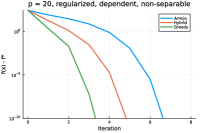
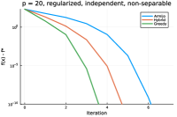
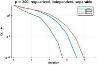
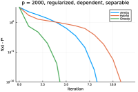
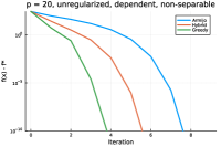
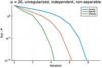
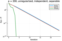
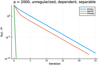
Figure 1: Comparison of Newton with Armijo backtracking, hybrid gradient-Newton, and greedy Newton on logistic regression problems with regularization (top row) and without regularization (bottom row). From left to right, in the bottom row the problems are convex, strongly-convex, strictly-convex, and convex (all problems in the top row are strongly-convex). The right two datasets are linearly separable and the left two datasets are non-separable.

In Figure 1 we compare Newton with Armijo backtracking, the hybrid of greedy gradient descent and pure Newton discussed in Section 2.4, and GN. We see that GN outperformed the other two methods in all settings. The performance gain was particularly large in the unregularized case for the two separable datasets (where the optimal solutions have infinite norm): in these cases the Armijo and hybrid methods performed poorly while GN achieved numerical accuracy extremely quickly (in 4 iterations and 1 iteration respectively). In these cases GN used step sizes much larger than 1, while for the other datasets GN initially used large step sizes but they quickly converged 1 (see Figure LABEL:fig:logregt). In Appendix LABEL:app:exp we report results based on real data which largely show similar trends.

4 Open Problems

Our experiments show that we can use Newton’s method more advantageously when we do not restrict the step size to be less than 1. However, our theory does not reflect the large performance increases we saw in practice. Below we list some open problems:

1. Section 2.1: can we prove that step sizes bigger than 1 improve the global rate?

2. Section 2.2: is the additional $\sqrt{L/\mu}$ term in the superlinear rate necessary?

3. Section 2.3: can we analyze the rate at which $\alpha_{k}$ converges to 1?

4. Section 2.4: can we justify why GN outperforms the theoretically-faster hybrid method?

5. Section 3: can we prove a faster rate for GN on separable problems?

We close by noting that a precise step size search could also be added to Newton’s method with cubic regularization and that this does not change the radius of superlinear convergence of that method (Appendix LABEL:app:cubic).

Appendix A Analysis of Greedy Newton

In this section, we prove the results in Sections 2.1-2.3. Our analyses are modifications of existing convergence analyses of the pure and backtracking Newton method [2; 11; 16] to use an exact line search.

A.1 Global Convergence of Greedy Newton

In this section we give the proof of Proposition 2.1. Our assumption is that $\nabla^{2}f(x_{k})$ is positive definite with eigenvalues in $[\mu,L]$. This implies that $\nabla^{2}f(x_{k})^{-1}$ is symmetric and positive definite with eigenvalues in $[1/L,1/\mu]$. Using these facts in a Taylor expansion gives f(x_k+1) & = f(x_k) + ∇f(x_k)^T(x_k+1-x_k) + 12(x_k+1-x_k)^T∇^2 f(z)(x_k+1-x_k) (for $z$ between $x_{k+1}$ and $x_{k}$)
≤f(x_k) + ∇f(x_k)^T(x_k+1-x_k) + L2∥x_k+1-x_k∥^2 ($\nabla^{2}f(z)\preceq LI$)
= f(x_k) - α_k ∇f(x_k)^T ∇^2f(x_k)^-1∇f(x_k)+ Lαk22∥∇^2f(x_k)^-1∇f(x_k)∥^2 ($x_{k+1}$ is Newton step eq:GN_update)
= f(x_k) - α_k ∇f(x_k)^T ∇^2f(x_k)^-1∇f(x_k)+ Lαk22∇f(x_k)^T∇^2 f(x_k)^-2∇f(x_k)
≤f(x_k) - α_k ∇f(x_k)^T ∇^2f(x_k)^-1∇f(x_k) + Lαk22μ ∇f(x_k)^T ∇^2 f(x_k)^-1∇f(x_k) ($\nabla^{2}f(x_{k})^{-1}\preceq(1/\mu)I)$
= f(x_k) - α_k(1 - αk2Lμ)∇f(x_k)^T∇^2f(x_k)^-1∇f(x_k) With an exact line search eq:newton_exactLS, we decrease the function by at least as much as choosing $\alpha_{k}=\mu/L$, so we have f(x_k+1) & ≤f(x_k) - μ2L∇f(x_k)^T ∇^2f(x_k)

References

- Bertsekas [2016] D. P. Bertsekas. Nonlinear Programming. Athena Scientific, 3 edition, 2016.
- Boyd and Vandenberghe [2004] S. Boyd and L. Vandenberghe. Convex Optimization. Cambridge, 2004.
- Burdakov [1980] O. P. Burdakov. Some globally convergent modifications of Newton’s method for solving systems of nonlinear equations. Doklady Akademii Nauk, 254(3):521–523, 1980.
- Deuflhard [2012] P. Deuflhard. A short history of Newton’s method. Documenta Mathematica, Optimization stories, pages 25–30, 2012.
- Golub and Van Loan [2013] Gene H Golub and Charles F Van Loan. Matrix computations. JHU press, 2013.
- Ivanova and Hildebrand [2023] A. Ivanova and R. Hildebrand. Optimal step length for the maximal decrease of a self-concordant function by the Newton method. Optimization Letters, pages 1–8, 2023.
- Jarre and Toint [2016] F. Jarre and P. L. Toint. Simple examples for the failure of Newton’s method with line search for strictly convex minimization. Mathematical Programming, 158(1-2):23–34, 2016.
- Mascarenhas [2007] W. F. Mascarenhas. On the divergence of line search methods. Computational & Applied Mathematics, 26:129–169, 2007.
- Narkiss and Zibulevsky [2005a] G. Narkiss and M. Zibulevsky. Sequential subspace optimization method for large-scale unconstrained problems. Technical report, Technion - Israel Institute of Technology, 2005a.
- Narkiss and Zibulevsky [2005b] G. Narkiss and M. Zibulevsky. Support vector machine via sequential subspace optimization. Technical report, Technion - Israel Institute of Technology, 2005b.
- Nesterov [2018] Y. Nesterov. Lectures on Convex Optimization, 2nd Ed. Springer, 2018.
- Nesterov and Polyak [2006] Y. Nesterov and B. Polyak. Cubic regularization of Newton method and its global performance. Math. Program., 108:177–205, 2006.
- Nocedal and Wright [2006] J. Nocedal and S. J. Wright. Numerical Optimization, 2nd Ed. Springer, 2006.
- Schmidt [2005] M. Schmidt. Minfunc: unconstrained differentiable multivariate optimization in Matlab, 2005.
- Shea and Schmidt [2023] B. Shea and M. Schmidt. Why line-search when you can plane-search? arXiv preprint, 2023.
- Sun [2021] Y. Sun. The happy optimist: Newton’s method I, 2021.
- Zibulevsky [2008] M. Zibulevsky. Sesop-tn: combining sequential subspace optimization with truncated Newton method, 2008.
- Zibulevsky [2010] M. Zibulevsky. SESOP_PACK: Matlab tool for sequential subspace optimization methods, 2010.