Make Prompts Adaptable: Bayesian Modeling
for Vision-Language Prompt Learning with Data-Dependent Prior

Abstract

Recent Vision-Language Pretrained (VLP) models have become the backbone for many downstream tasks, but they are utilized as frozen model without learning. Prompt learning is a method to improve the pre-trained VLP model by adding a learnable context vector to the inputs of the text encoder. In a few-shot learning scenario of the downstream task, MLE training can lead the context vector to over-fit dominant image features in the training data. This overfitting can potentially harm the generalization ability, especially in the presence of a distribution shift between the training and test dataset. This paper presents a Bayesian-based framework of prompt learning, which could alleviate the over-fitting issues on few-shot learning application and increase the adaptability of prompts on unseen instances. Specifically, modeling data-dependent prior enhances the adaptability of text features for both seen and unseen image features without the trade-off of performance between them. Based on the Bayesian framework, we utilize the Wasserstein Gradient Flow in the estimation of our target posterior distribution, which enables our prompt to be flexible in capturing the complex modes of image features. We demonstrate the effectiveness of our method on benchmark datasets for several experiments by showing statistically significant improvements on performance compared to existing methods. The code is available at https://github.com/youngjae-cho/APP.

Introduction

Recently, Vision-Language Pretrained models (VLP) (Radford et al. 2021; Jia et al. 2021) have been used as backbones for various downstream tasks (Shen et al. 2022; Ruan, Dubois, and Maddison 2022), and the pre-trained models have shown successful adaptation. Since these pre-trained models are used as-is in downstream tasks, prompt learning adds a context vector to the input of pre-trained model, so the context vector becomes the learnable parameter to improve the representation from the pre-trained model (Zhou et al. 2022b) for the downstream task. For instance, a text input is concatenated to a context vector, and the new text input could be fed to the text encoder. The learning of context vector comes from the back-propagation after the feed-forward of the concatenated text input. Since there is only a single context vector without being conditioned by inputs, the inferred value of context vector becomes a static single context defined for the given downstream task.

Whereas improving parameter-frozen VLP models by additional input context vector is a feasible solution, it can potentially overfit to a dense area of image features in few-shot learning. Since text features are hard to capture the multi-modes of image features in MLE training, it could fail to infer the minor area of image features, eventually degrading the performance. In addition, MLE training undermines the generalization capability of VLP models especially when there is a distribution shift between the training and testing (Zhou et al. 2022a). Although several input-conditioned prompt learning (Zhou et al. 2022a; Derakhshani et al. 2023) tried to generalize unseen datasets, it inevitably undermines the performance of seen datasets.

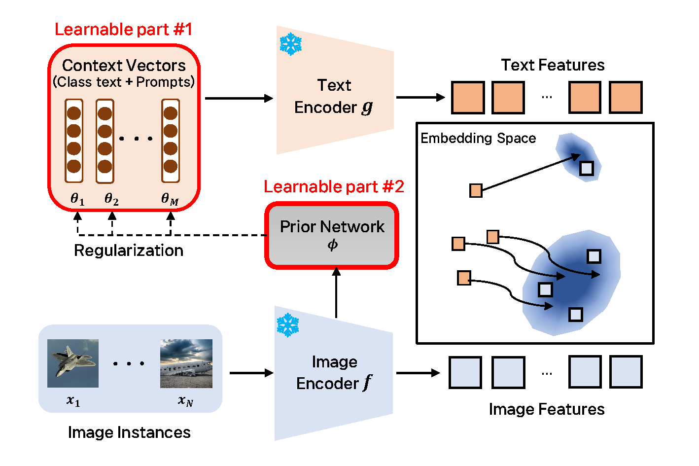
(a) Structure view of APP

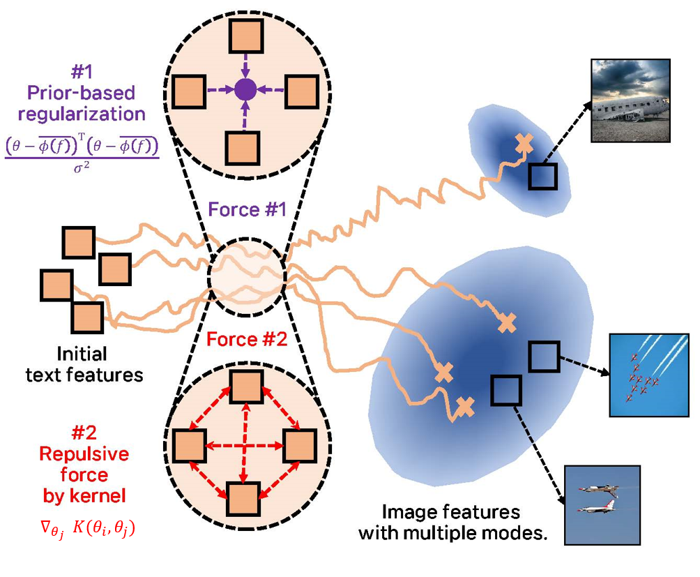
(b) Learning dynamics of APP

Figure 1: Structure (left) and learning dynamics (right) of APP. Multiple context vectors are particles of approximated distribution and image conditioned prior can guide the context vector to capture the multi modes.

To alleviate the impact of uncertainty arising from a few-shot learning scenario, our paper proposes Adaptive Particle-based Prompt Learning (APP), which utilizes a Bayesian inference for prompt learning with a data-dependent prior as shown in Figure 1. Through regularization using this data-dependent prior, the context vector is directed toward capturing the diverse modes in image features among the seen data instances. Additionally, we approximate the posterior distribution via Wasserstein Gradient Flow to enhance the flexibility of our text features to infer the complex image features. Furthermore, we extend the modeling of the data-dependent prior to unseen test instances to adapt the distribution shift. This adaptation of the context vector to the unseen instances enhances the model’s resilience in the face of distribution shifts, providing robustness to these variations.

We summarize our contributions in two aspects.

1. Enhancing Flexibility of Prompt: By approximating prompt posterior with Wasserstein Gradient Flow, our context vectors can be more flexibly utilized to infer the complex image feature spaces.

2. Enhancing Adaptability of Prompt: By modeling data-dependent prior based on the image feature information, text features capture the multi-modes of seen image features and adapt to unseen image features, which leads to the improved performances of seen and unseen datasets without trade-off.

Preliminary

Formulation of Prompt Learning

Deterministic Prompt Learning

The goal of prompt learning, i.e. CoOp (Zhou et al. 2022b), is to facilitate adaptation of a given Vision-Language Pretrained model for a target task through learning arbitrary context vectors. In this setting, the pre-trained VLP model is frozen under the prompt learning task, and the additional learnable input is added to text inputs. Finally, the learning gradient is obtained from adapting the target task, a.k.a. downstream task. When we define $(X,Y)$ as a pair of image and its label (i.e. text phrase), Eq. Deterministic Prompt Learning shows a log-likelihood of prompt learning in the image classification.

$$\mathcal{L}_{CE}(\theta,X,Y)=-\log p(Y|X,\theta)$$

$$=-\sum_{i=1}^{N}\{\log({\exp(\text{sim}(g(\theta,y_{i}),f(x_{i}))/\tau)\over\sum_{k=1}^{C}\exp(\text{sim}(g(\theta,y_{k}),f(x_{i}))/\tau)})\}$$ (1)

Here, $f$ and $g$ are image and text encoders from VLP models, respectively; and they are frozen in prompt learning. Therefore, the only learnable part is $\theta$, which is a context vector. $\theta\in\mathbb{R}^{d}$ is learned as a unique vector for each downstream task without discriminating the data instances. Since $g$ is often implemented as a transformer to take sequential inputs of any length, $g$ does not need to be modified to accept $y$ and $\theta$. Additionally, $\text{sim}(\cdot)$ represents cosine similarity, and $\tau$ is the annealing temperature.

From Eq. Deterministic Prompt Learning, we define the prompt as $\{\theta,y_{i}\}$, which is the concatenation of the context vector and the label. By minimizing Eq. Deterministic Prompt Learning, $\theta$ is learned to maximize the alignment of the space between the image feature $f(x)$ and the text feature $g(\theta,y_{i})$. Therefore, the learnable part of prompt learning contributes from the input space side, rather than the frozen VLP model parameters. There were some follow-up researches on CoOp. For example, CoCoOp (Zhou et al. 2022a) extended CoOp by learning the image-conditional context vector as $\theta+\phi(f(x_{i}))$, where $\phi$ is a neural network to map image feature to the prompt space.

Probabilistic Prompt Learning

Given a few instance of training dataset, the point estimate of text feature given prompt is hard to capture unseen image feature. ProDA (Lu et al. 2022) is the first probabilistic model, where the text feature-given prompt is approximated as a Gaussian distribution with a regularizer to enhance the diversity of text feature. PLOT (Chen et al. 2023) formulates the prompt learning as optimal transport, where image and text features are defined as a discrete distribution by Dirac measure. The text features, given as multiple prompts, are assigned to the locality of image features to learn diverse semantics.

Bayesian Probabilistic Prompt Learning

Since MLE training can induce overfitting with a few training dataset, Bayesian inference is needed to mitigate the high data variance from such a limited dataset. BPL (Derakhshani et al. 2023) is the first prompt learning model from the view of Bayesian inference, which uses variational inference to approximate the posterior distribution with a parameterized Gaussian distribution. The objective function of BPL is defined as follows:

$$\operatorname{\mathbb{E}}_{q(r|X)}[\log(p(Y|X,\theta,r))]-D_{KL}(q(r|X)||p(r))$$ (2)

where $r$ is a random variable conditioned on $X$, and $r$ is added to a deterministic $\theta$ to turn it into a random variable, which is a reparameterization trick. In detail, the distribution of $r$ is given by $q(r|X)$, which is a Gaussian distribution parameterized by $m(f(X))$ and $\Sigma(f(X))$, where $m(f(X))$ and $\Sigma(f(X))$ are functions of the image feature $f(X)$. The prior distribution over $r$ is $p(r)$, which is a standard Gaussian distribution $N(0,I)$.

Wasserstein Gradient Flow

Bayesian inference is a solution to mitigate the uncertainty from modeling the posterior distribution of parameters. Often, the hurdle of the Bayesian inference is the inference of the posterior distribution, which could be difficult, i.e. modeling either prior or likelihood to be flexible without being conjugate to each other. For improving the posterior distribution to be flexible and multi-modal, we need an inference tool for this complex posterior distribution.

For instance, the JKO scheme (Jordan, Kinderlehrer, and Otto 1998) interprets variational inference as gradient flow, which minimizes the KL divergence between the variational distribution $q$ and the true posterior distribution $\pi\propto\exp(-V(\theta))$ in Wasserstein Space, where $V(\theta)$ is an energy function of posterior distribution. The learning objective of this variational posterior inference $F(q)$ becomes the KL Divergence as follows.

$$F(q)\coloneqq D_{KL}(q||\pi)\approx\operatorname{\mathbb{E}}_{q}[V(\theta)+\log q]$$ (3)

To compute the steepest gradient of $F(q)$, we define the Wasserstein Gradient Flow (WGF) as follows:

Definition 1.

Suppose we have a Wasserstein space $\mathcal{W}_{2}=(\mathcal{P}_{2}(\mathbb{R}^{d}),W_{2})$, $\mathcal{P}_{2}(\mathbb{R}^{d})=\{\mu\in\mathcal{P}_{2},\int||\theta||^{2}d\mu(\theta)<\infty\}$, $W_{2}(\mu_{1},\mu_{2})=min_{\omega\in\Pi(\mu_{1},\mu_{2})}\int{||\theta-\theta^{\prime}||}^{2}d\omega(\theta,\theta^{\prime})$.

A curve of $\mu_{t}$ is a Wasserstein Gradient Flow for functional $F$, if it satisfies Eq. 4.

$$\partial_{t}\mu_{t}=\nabla\cdot(\mu_{t}\nabla_{\theta}{\delta F(\mu_{t})\over\delta\mu})=\nabla\cdot(\mu_{t}\nabla_{W_{2}}F(\mu_{t}))$$ (4)

WGF can be discretized as Stochastic Gradient Langevin Dynamics (SGLD) (Welling and Teh 2011; Chen et al. 2018) as Eq. 5, where each particle $\theta$ follows the true posterior distribution $\pi$ with Gaussian perturbation.

$$\theta_{t+1}^{i}=\theta_{t}^{i}-h(\nabla_{\theta_{t}^{i}}V(\theta^{i}_{t}))+\sqrt{2h}\epsilon,\epsilon\sim N(0,I)$$ (5)

Whereas the Gaussian noise can assure the diversity of parameters, the learning can be unstable, when the learning rate is high.

Hence, this paper relies on Stein Variational Gradient Descent (SVGD) (Liu and Wang 2016), which is a version of Wasserstein Gradient Flow with Reproducing Kernel Hilbert Space (RKHS) (Chen et al. 2018). In SVGD, interaction between particles $\theta_{i}$ guarantees their convergence to true posterior distribution with forcing diversity.

$$\theta_{t+1}^{i}=\theta_{t}^{i}-{h\over M}\sum_{j=1}^{M}K(\theta_{t}^{i},\theta_{t}^{j})\nabla_{\theta_{t}^{j}}V(\theta_{t}^{j})-\nabla_{\theta_{t}^{j}}K(\theta_{t}^{i},\theta_{t}^{j})$$ (6)

By using SVGD to approximate true posterior distribution, context vectors $\theta^{j}$ can be optimized to follow the true posterior distribution, effectively capturing a representation space of the image features.

Data-Dependent Prior

In a Bayesian neural network, the prior is commonly chosen as the Standard normal distribution, i.e. BPL, which is data-independently initialized with zero means. Since such distribution does not include any information on data, it only regularizes the context vector in the neighbor of zero-mean. In many domains (Li et al. 2020; gil Lee et al. 2022), the data-dependent prior is utilized to improve the prior knowledge more informative.

This paper utilizes the data-dependent prior for prompt learning, which is not restricted to the standard Gaussian distribution. Specifically, this paper derives the prior distribution to be dependent on image features, which can have multiple modes in their distributions.

Method

This section introduces adaptive particle-based prompt learning (APP) by enumerating the model formulation and by explaining its inference method.

Formulation of Prompt Posterior Distribution

Following the CoOp formulation (Zhou et al. 2022b), we additionally reformulate the posterior distribution of context vector $\theta$ as Eq. Formulation of Prompt Posterior Distribution.

$$\pi(\theta)=p(\theta|X,Y) ={p(Y|X,\theta)p(\theta|X)p(X)\over p(X,Y)}$$

$$\propto p(Y|X,\theta)p(\theta|X)$$ (7)

$\pi(\theta)$ is true posterior distribution, which is factorized with likelihood $p(Y|X,\theta)$ and conditioned prior $p(\theta|X)$. For likelihood Eq. Deterministic Prompt Learning, we follow the formulation of CoOp, Eq. Deterministic Prompt Learning, and we propose the image feature conditioned prior Eq. 8, where mean is parametrized as $\phi$ and $\overline{\phi(f)}\coloneqq{1\over N}\sum_{i=1}^{N}\phi(f(x_{i}))$. We set the standard deviation of prior $\sigma$ as a hyper-parameter.

$$\log p(\theta|X)\propto-{(\theta-\overline{\phi(f)})^{T}(\theta-\overline{\phi(f)})\over\sigma^{2}}$$ (8)

Bayesian Adaptation of Prompt to Test data

In few-shot learning, there is uncertainty on whether the test data will follow the distribution of training data or not. If there is a difference between the two data distributions, such a difference will harm the generalization ability of VLP model. To model the uncertainty from the mismatch between training and test datasets in the few-shot learning framework, we reformulate the posterior distribution to consider the uncertainty of a test image $x^{\prime}$. Since training and test datasets are i.i.d sample; and because the prior is assumed to follow the Gaussian distribution; we derive the posterior distribution as Eq.Bayesian Adaptation of Prompt to Test data.

$$\pi(\theta)=p(\theta|X,Y,x^{\prime}) ={p(Y|X,\theta)p(\theta|X)p(\theta|x^{\prime})p(X)\over p(X,Y)}$$

$$\propto\underbrace{p(Y|X,\theta)p(\theta|X)}_{Training}\underbrace{p(\theta|x^{\prime})}_{Testing}$$ (9)

After approximating the Eq.Formulation of Prompt Posterior Distribution, we adapt the context vector $\theta$ with test data-dependent prior.

Variational Inference for Prompt Posterior

Since Eq. Formulation of Prompt Posterior Distribution is not tractable, we approximate the posterior distribution of $\pi$, using particle-based variational inference. Suppose that $q$ is a probabilistic measure of variational distribution, which generates the context vector $\theta$, in Wasserstein space. Eq. 11 defines the optimization problem to approximate the model posterior distribution by the variational distribution.

$$V(\theta)\coloneqq-\log p(Y|X,\theta)-\log p(\theta|X)$$ (10)

$$F(q)\coloneqq D_{KL}(q||\pi)\approx\operatorname{\mathbb{E}}_{q}[V(\theta)+\log q]$$ (11)

To define the steepest direction of Eq. 11, we follow Wasserstein Gradient Flow Eq.4. By solving the Wasserstein Gradient Flow in Reproducing Kernel Hilbert Space (RKHS), we can define the following Wasserstein Gradient for variational distribution $q$, where the linear operator $\mathcal{K}_{q}T(\theta)\coloneqq\operatorname{\mathbb{E}}_{\theta^{\prime}\sim q}[K({\theta},{\theta^{\prime}})T({\theta^{\prime}})]$.

$$\partial_{t}q_{t}=\nabla\cdot(q_{t}\mathcal{K}_{q}\nabla_{q}{\delta F(q)\over\delta q})$$ (12)

Following the Continuity Equation, we can define the evolving path of $\theta_{t}\sim q_{t}$ as follows.

$$\partial_{t}\theta_{t} =-\mathcal{K}_{q}\nabla_{\theta}({\delta F(q)\over\delta q})$$

$$=-[\int K({\theta},{\theta^{\prime}})\nabla_{\theta^{\prime}}V(\theta^{\prime})dq-\int\nabla_{\theta^{\prime}}K(\theta,\theta^{\prime})dq]$$ (13)

By discretizing Eq. Variational Inference for Prompt Posterior, we derive the Stein Variational Gradient Descent (Liu and Wang 2016), where each context vector $\theta^{j}$ can be optimized as follows.

$$\theta_{t+1}^{i}=\theta_{t}^{i}-{h\over M}\sum_{j=1}^{M}[K(\theta_{t}^{i},\theta_{t}^{j})\nabla_{\theta_{t}^{j}}V(\theta_{t}^{j})-\nabla_{\theta_{t}^{j}}K(\theta_{t}^{i},\theta_{t}^{j})]$$ (14)

For Eq. 14, the first term can be interpreted as a smoothing gradient between context vectors $\theta^{j}$ and assure the convergence toward the true posterior distribution. The second term can be interpreted as the repulsive force between context vectors $\theta^{j}$ and guide the text features can cover the multi modes sparsely.

Parameter Training of Data-Dependent Prior

Since the prior has the parametrized mean $\phi$, we pre-train the $\phi$, which can map the image feature on the prompt space. To preserve the image feature information within our prior distribution, we propose to maximize the mutual information $I\left(\phi\left(f\left(x\right)\right);f(x)\right)$. In other words, this mutual information encourages the prior to capture the dependencies between the image features and the parameter of the prompt distribution. Due to the data processing inequality (Beaudry and Renner 2012), we derive inequality as follows:

$$I(\phi(f(X));f(X))\geq I(g(\phi(f(X)),\cdot);f(X))$$ (15)

where $\phi$ can be learned to maximize the mutual information.

Proposition 1.

Suppose that the Markov chain assumption holds as $f(X)\rightarrow\phi(f(X))\rightarrow g(\phi(f(X)),\cdot)$, then the lower bound of the mutual information, $I(f(X);\phi(f(X)))$, is derived as follows:
$I(f(X);\phi(f(X)))\geq I(f(X);g(\phi(f(X)),\cdot))\geq\log C-\mathcal{L}_{CE}(\phi(f(X)),X,Y)$

Based on Proposition 1, we can maximize the mutual information by minimizing the cross entropy. The full training scenario is reported in Algorithm 1.

Adaptation $\theta$ with Test Data-Dependent Prior

Following the training of the posterior distribution as described in Eq. Formulation of Prompt Posterior Distribution, we extend our approach to accommodate an unseen data instance, $x^{\prime}$, within the posterior distribution. This involves updating the context vector $\theta\sim q$ through a linear combination with the prior mean $\phi(f(x^{\prime}))$. For the sake of simplicity, we perform a weighted average of the text features, which can be outlined as follows. The adaptation scenario is reported in Algorithm 2.

$$g(\theta^{*},y)=\alpha g(\theta,y)+(1-\alpha)g(\phi(f(x^{\prime})),y)$$ (16)

Algorithm 1 Training Scenario of APP

1:Input: Dataset $\mathcal{D}=\{X,Y\}$, Context vector $\theta^{i}$, Prior Network $\phi$

2:while  not converged do

3:     Compute $\mathcal{L}_{CE}(\phi(f(X)),X,Y)$

4:     Update $\phi_{t+1}=\phi_{t}-h\nabla_{\phi}\mathcal{L}_{CE}$

5:end while

6:while  not converged do

7:     Compute $V(\theta)=-\log p(Y|X,\theta)-\log p(\theta|X)$

8:     Update $\theta_{t+1}^{i}=\theta_{t}^{i}-{h\over M}\sum_{j=1}^{M}[K(\theta_{t}^{i},\theta_{t}^{j})\nabla_{\theta_{t}^{j}}V(\theta_{t}^{j})-\nabla_{\theta_{t}^{j}}K(\theta_{t}^{i},\theta_{t}^{j})]$ $,\forall{i\in[1,...,M]}$

9:end while

Algorithm 2 Test Scenario of APP

1:Input: Test image instance $x^{\prime}$, Context vector $\theta^{i}$, Prior Network $\phi$

2:Training as Algorithm 1

3:Compute $g(\theta^{*},y_{j})$ as Eq.16, $\forall{j\in[1,..,K]}$

4:$y^{\prime}=\text{argmax}_{y_{j}}\text{sim}(g(\theta^{*},y_{j}),f(x^{\prime}))$

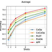
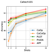
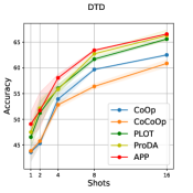
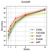
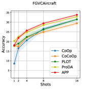
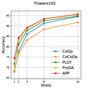
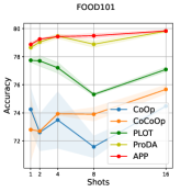
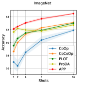
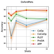
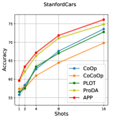
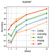
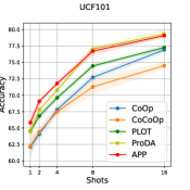
Figure 2: Result of Few-shot Classification. We conduct three-replicated experiments.

Results

Experiment Settings

We conduct three distinct experiments; Few-shot classification, domain generalization of ImageNet, and base-to-new generalization following PLOT (Chen et al. 2023). For Few-shot classification, we conduct 11 image datasets, including Caltech101 (Fei-Fei, Fergus, and Perona 2004), DTD (Cimpoi et al. 2014), EuroSAT (Helber et al. 2019), FGVCAircraft (Maji et al. 2013), Oxford 102 Flower (Nilsback and Zisserman 2008), OxfordPets (Parkhi et al. 2012), Food101 (Bossard, Guillaumin, and Van Gool 2014), StanfordCars (Krause et al. 2013), Sun397 (Xiao et al. 2010), UCF101 (Soomro, Zamir, and Shah 2012), and ImageNet (Deng et al. 2009). We followed the training setting of PLOT (Chen et al. 2023), where the training shots are chosen in 1, 2, 4, 8, 16 shots, and we train 50, 100, 100, 200, and 200 epochs for each shot. For ImageNet, we train the prompts in 50 epochs for all shots. Before the training context vector $\theta$, we train the prior mean $\phi$ in 10, 20, 20, 40, and 40 epochs for each shot. For domain generalization of ImageNet, we train prompts about ImageNet as a source dataset and report the accuracy of the source dataset and target datasets, including ImageNetV2 (Recht et al. 2019), ImageNet-A (Hendrycks et al. 2021b), ImageNet-R (Hendrycks et al. 2021a), and ImageNet-Sketch (Wang et al. 2019). For base-to-new generalization, we train prompts using 16 shots for each of 11 datasets for the base class and report the performance of base and new classes.

As a common setting, we conduct three replicated experiments to report the performances, and we use CLIP (Jia et al. 2021) as the backbone network, where ResNet50 (He et al. 2016) is chosen as the image encoder. All context vectors are vectors of 16 dimensions, which are sampled from $N(0,0.02I)$, and class information is inserted at the end position of context vectors. We fixed the precision $1/\sigma^{2}$ as 1.0 for all settings, and RBF kernel is used for $K$. The adaptation weight $\alpha$ is chosen as 0.9 for few-shot classification, and 0.7 for generalization experiments. We report more details of the setting in the Appendix.

Baselines

We compare the performance of our method, APP with CoOp (Zhou et al. 2022b), CoCoOP (Zhou et al. 2022a), PLOT (Chen et al. 2023), and ProDA (Lu et al. 2022). We do not include BPL (Derakhshani et al. 2023) as our baselines due to reasons in the Appendix. We initialize the four context vectors for PLOT, ProDA, and APP randomly.

Few-Shot Classification

Quantitative Analysis

Figure 2 indicates that our method outperforms baselines on all benchmark datasets on average, where our performance is superior to 45 out of 55 experiment cases (11 datasets $\times$ 5 shots). The advantage of APP stands out in Caltech101, DTD, EuroSAT, and ImageNet, which consist of more diverse images. Since the data-dependent prior and the repulsive force of Eq. 14 enable text features to infer the multi-modes of image features, our context vectors are learned to capture the diverse semantics of image features.

Qualitative Analysis

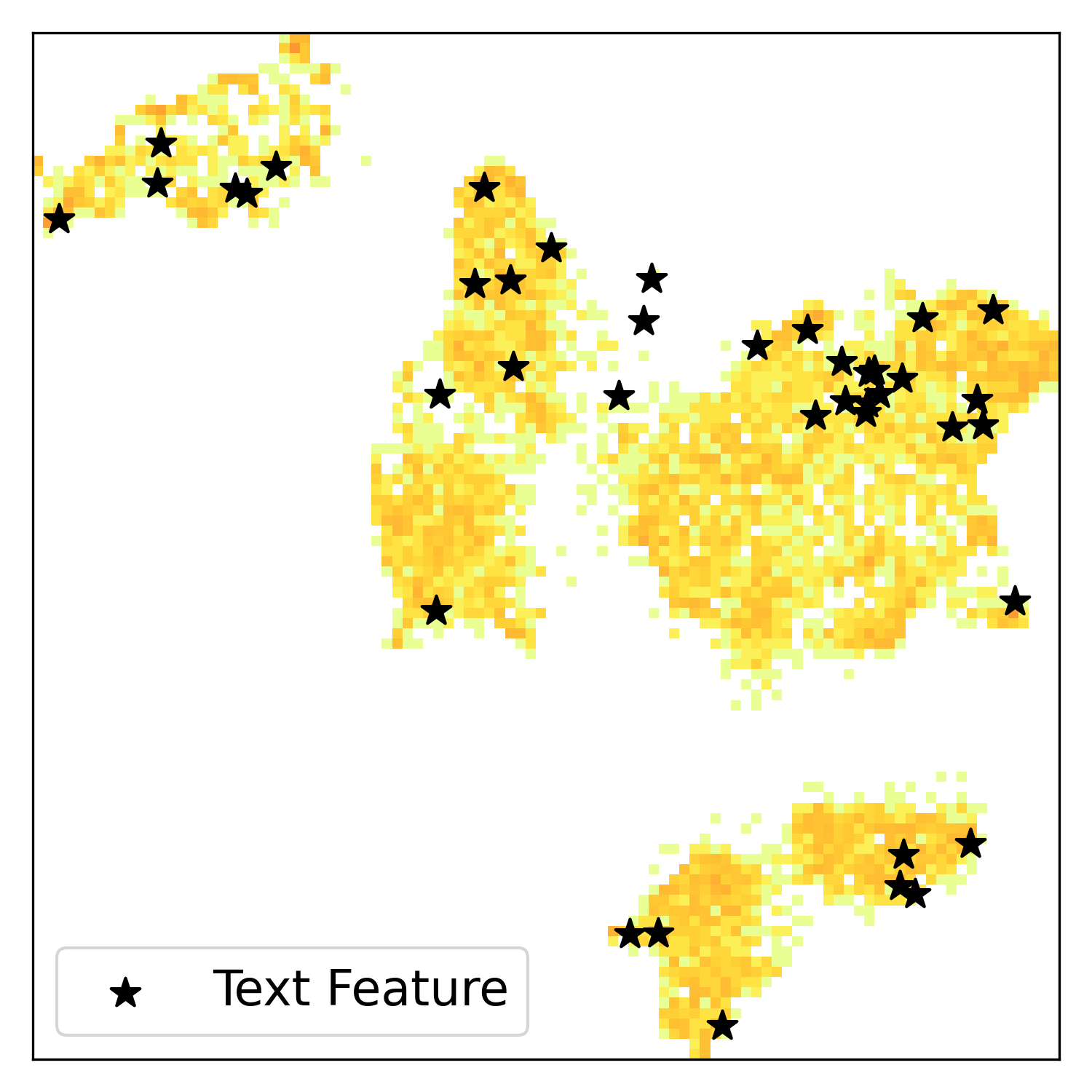
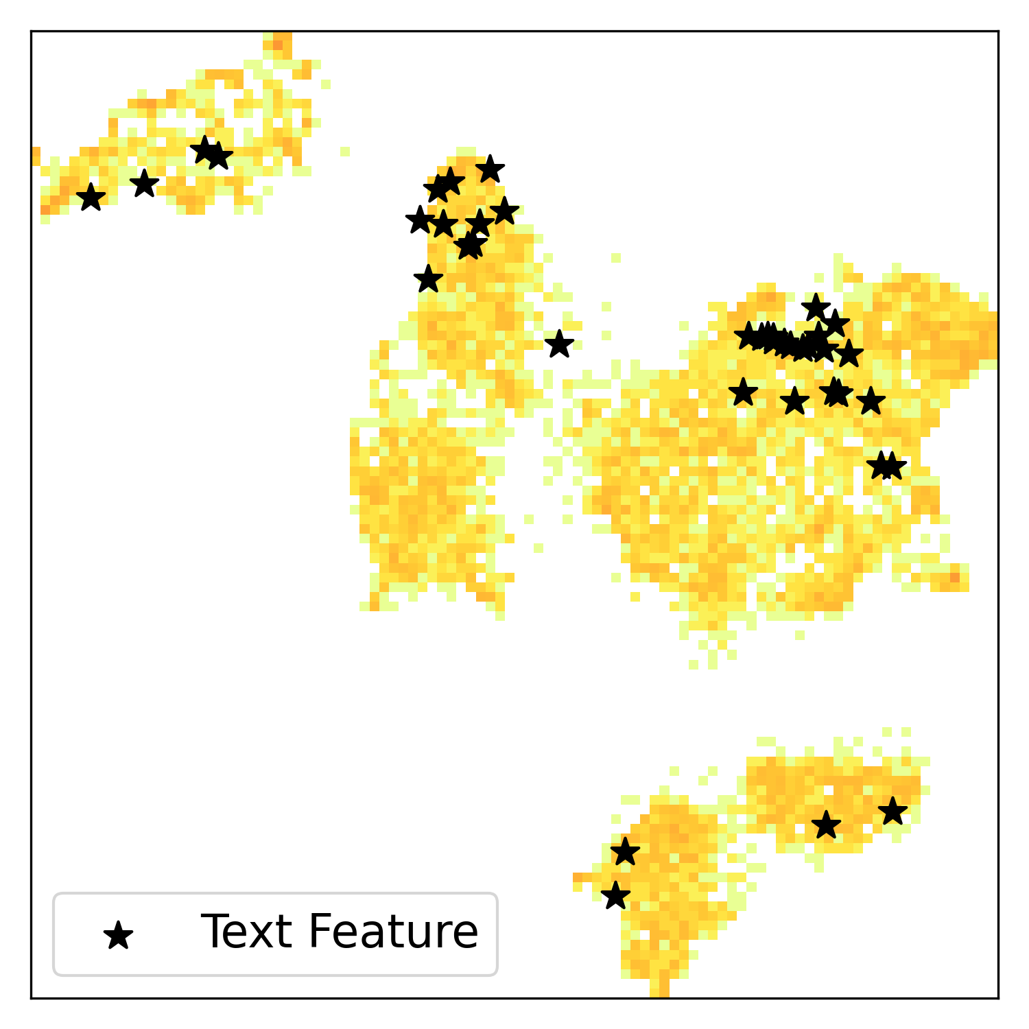
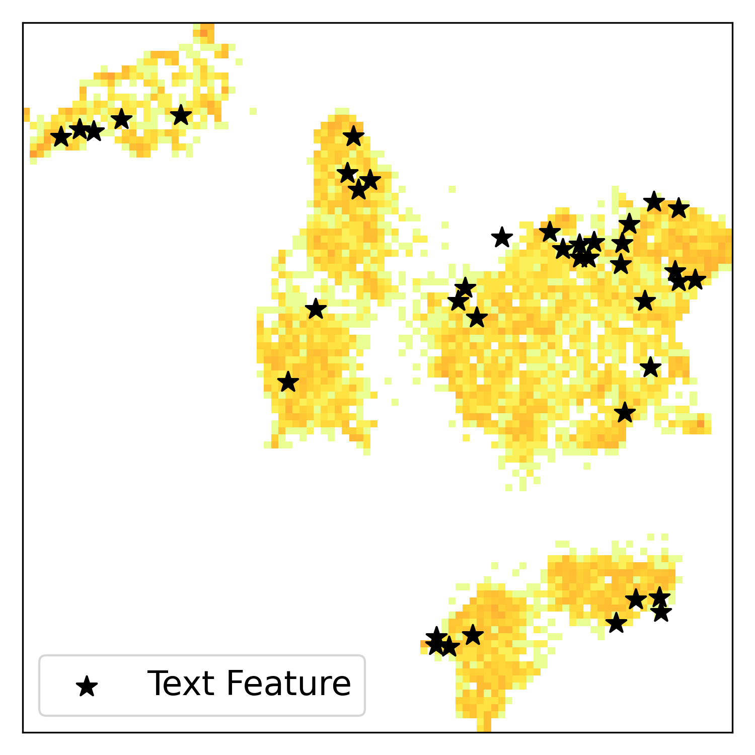
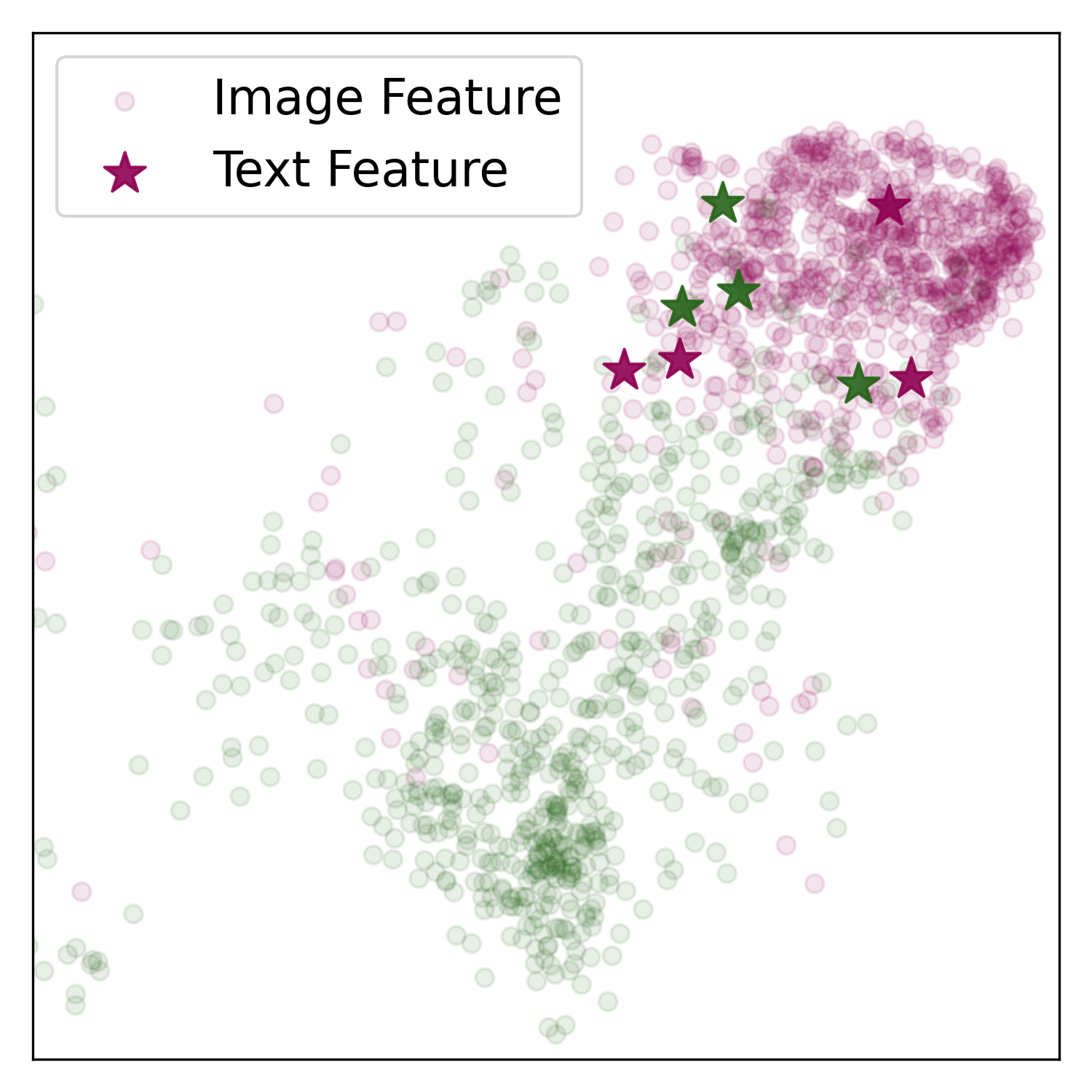
(a) PLOT

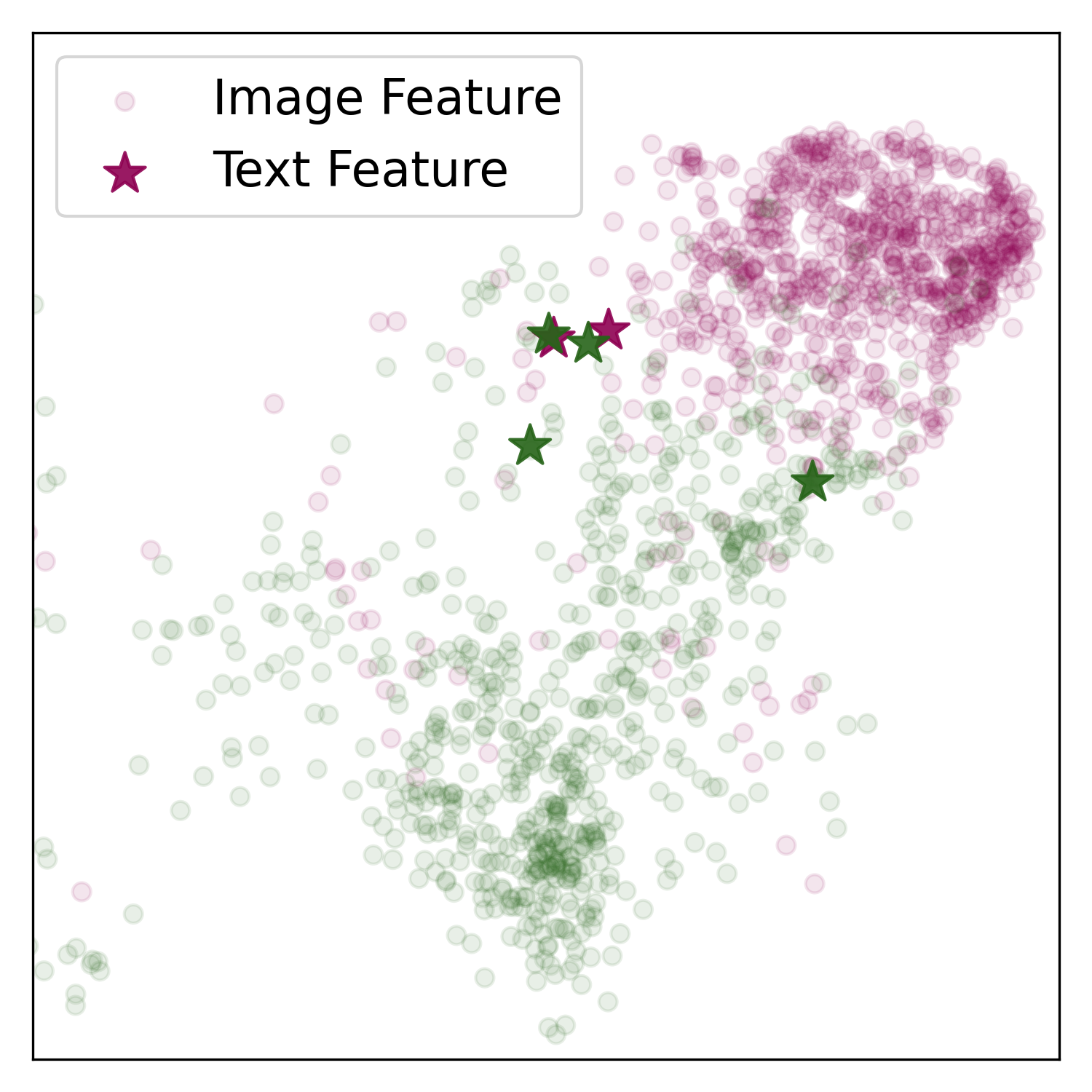
(b) ProDA

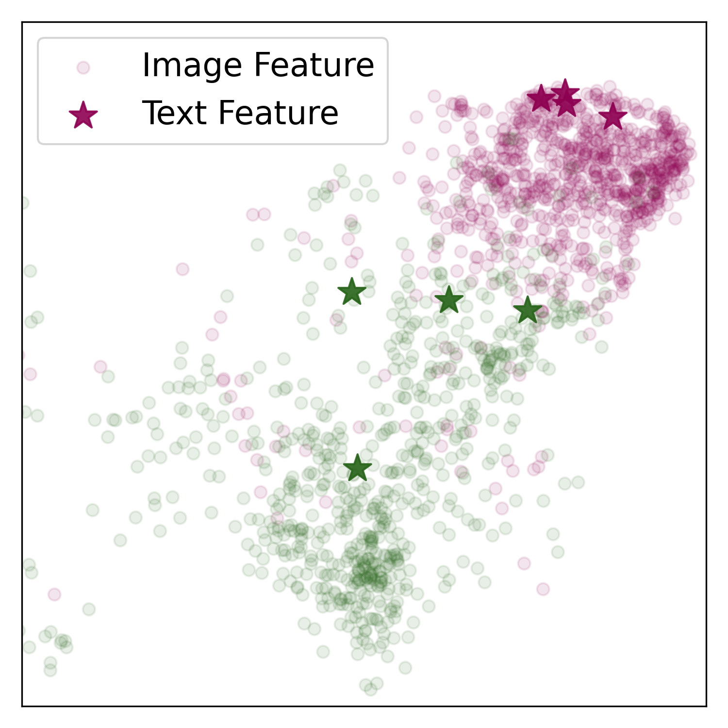
(c) APP

Figure 3: Umap visualization about image features and text features for EuroSAT. (Upper) Histograms correspond to image features and $\star$ means text features of all classes. (Lower) Image and text features of arbitrary two classes. The color coding corresponds to each class.

To demonstrate the efficacy of our method in capturing intricate image features, we provide visualizations of both image features ($f(x_{i})$) and text features ($g(\theta_{j},y_{i})$). In Figure 3, we present Umap (McInnes, Healy, and Melville 2018) representations for EuroSAT test dataset. The upper figures depict image and text representations of all classes. A richer yellow hue indicates a denser allocation of image features. Our method, APP, well captures and comprehensively spans various modes within image features. The lower figures spotlight two arbitrarily selected classes, revealing how APP’s text features harmoniously align with the image features of each class. This alignment is particularly pronounced in comparison to other methods.

Table 1 provides the numerical analysis of the alignment between text feature representations from our method and image feature modes. We fitted k-means clustering on the test image features with k as a hyperparameter. Then, we counted the number of prompts assigned on each cluster, which will be similar for all clusters if prompts are adequately assigned to several modes of image features. In this context, we present the variance of prompt counts and show that text prompt representations of APP are well distributed across image feature representations.

Table 1: Variance of the number of text feature representations assigned to each cluster after fitting k-means clustering to image features. Bold means the smallest of each column.

Methods	k (Number of clusters)
	5	6	7	8	9	10
PLOT	26.0	27.6	11.9	7.5	8.5	7.8
ProDA	53.2	26.6	25.3	12.0	9.8	9.0
APP	25.2	21.9	9.9	6.3	4.0	2.6

Ablation Study

We show two ablation studies, considering our method and the number of prompts.

To identify the key enabler, we conduct additional ablation studies for APP by experimenting on 1) data-dependent prior and 2) Stein Variational Gradient Descent (SVGD). For all cases, four context vectors are initialized, and we select MLE training as the baseline optimized by SGD. Table 2 shows the posterior approximation with data-dependent prior improved performances generally than MLE Training. SVGD shows a more robust performance in a few data instances than SGD. The posterior approximation by SVGD also shows consistently better performance, outperforming in Caltech101 and EuroSAT dataset.

Table 2: An ablation study about our method, APP. Experiments are replicated over three times.

Dataset	Methods	Number of shots
		1	2	4
Caltech101	SGD	$89.87\pm 0.02$	$90.29\pm 0.20$	$91.00\pm 0.29$
	SVGD	$89.90\pm 0.07$	$90.56\pm 0.10$	$91.02\pm 0.29$
	SGD+Prior	$90.26\pm 0.21$	$90.70\pm 0.25$	$91.01\pm 0.14$
	SVGD+Prior (APP)	$\mathbf{90.30\pm 0.33}$	$\mathbf{90.87\pm 0.25}$	$\mathbf{91.05\pm 0.45}$
EuroSAT	SGD	$56.43\pm 2.31$	$63.93\pm 2.85$	$72.63\pm 2.74$
	SVGD	$58.93\pm 4.28$	$64.36\pm 3.16$	$73.64\pm 2.00$
	SGD+Prior	$59.96\pm 4.77$	$63.99\pm 2.88$	$72.63\pm 2.76$
	SVGD+Prior (APP)	$\mathbf{60.04\pm 2.08}$	$\mathbf{66.02\pm 2.70}$	$\mathbf{74.08\pm 2.23}$
Food101	SGD	$78.53\pm 0.14$	$78.88\pm 0.09$	$78.88\pm 0.25$
	SVGD	$78.51\pm 0.12$	$78.86\pm 0.07$	$78.87\pm 0.26$
	SGD+Prior	$78.81\pm 0.16$	$79.15\pm 0.07$	$79.32\pm 0.08$
	SVGD+Prior (APP)	$\mathbf{78.87\pm 0.17}$	$\mathbf{79.25\pm 0.06}$	$\mathbf{79.43\pm 0.10}$

We also carry out additional experiments varying the number of prompts to explore the influence of samples within the posterior distribution as table 3. While there is a tendency for higher performance with an increased number of prompts, please note that the performance can sufficiently be achieved with approximately four prompts.

Table 3: An ablation study with regard to the number of prompts (M). Experiments are replicated over three times.

Dataset	M	Number of shots
		1	2	4
Caltech101	2	$89.19\pm 0.20$	$90.08\pm 0.22$	$90.67\pm 0.69$
	4	$\mathbf{90.30\pm 0.33}$	$\mathbf{90.87\pm 0.25}$	$91.05\pm 0.45$
	8	$90.18\pm 0.28$	$90.33\pm 0.29$	$\mathbf{91.38\pm 0.16}$
EuroSAT	2	$52.06\pm 4.98$	$60.65\pm 3.00$	$71.19\pm 1.78$
	4	$\mathbf{{60.04\pm 2.08}}$	$\mathbf{66.02\pm 2.70}$	$74.08\pm 2.23$
	8	$58.60\pm 2.35$	$64.22\pm 5.32$	$\mathbf{74.32\pm 1.97}$
Food101	2	$78.27\pm 0.16$	$78.74\pm 0.09$	$78.93\pm 0.12$
	4	$78.87\pm 0.17$	$79.25\pm 0.06$	$79.43\pm 0.10$
	8	$\mathbf{78.90\pm 0.21}$	$\mathbf{79.29\pm 0.09}$	$\mathbf{79.45\pm 0.12}$

Time and Memory Complexity Comparison

In this paragraph, we compare the time and memory complexity between APP and CoCoOp. This comparison aims for showing the appropriateness of prompt learning in the context of efficiency. While both data-dependent prior and conditioned prompts share similarities in Figure 1(a), Table 4 underscores the fact that data-dependent priors exhibit efficiency and effectiveness. This is because the regularization process of the data-dependent prior does not require gradient updates.

Table 4: Time complexity for Caltech101. M means the number of prompts. $-$ is a training failure due to the memory issue. BS means Batch Size and Acc represents accuracy.

Methods	BS	Memory (GB)	Time (s)	Acc ($\%$)
CoCoOp	10	20	289	84.4
(M=1)	128	-	-	-
APP	10	7.2	260	89.3
(M=4)	128	9.6	112	90.2

Table 5: Test accuracies ($\%$) of the unseen classes generalization settings. H means the harmonic mean between the base accuracy and the new accuracy. Bold means the best accuracy of each column. We report the mean accuracy with three times replications due to the space issue.

Method	Base	New	H
CoCoOp	$71.7$	$53.6$	$61.4$
PLOT	$82.2$	$60.5$	$69.7$
ProDA	$82.4$	$63.6$	$71.8$
APP	$\mathbf{83.0}$	$\mathbf{65.8}$	$\mathbf{73.4}$

(a) Average

Method	Base	New	H
CoCoOp	$\mathbf{95.2}$	$87.4$	$91.2$
PLOT	$94.7$	$88.1$	$91.3$
ProDA	$\mathbf{95.2}$	$86.8$	$90.8$
APP	$\mathbf{95.2}$	$\mathbf{91.0}$	$\mathbf{93.0}$

(b) Caltech101

Method	Base	New	H
CoCoOp	$74.6$	$38.9$	$51.1$
PLOT	$78.1$	$42.7$	$55.2$
ProDA	$78.0$	$47.0$	$58.6$
APP	$\mathbf{78.4}$	$\mathbf{48.9}$	$\mathbf{60.2}$

(c) DTD

Method	Base	New	H
CoCoOp	$91.4$	$35.6$	$51.3$
PLOT	$92.9$	$39.3$	$55.2$
ProDA	$89.6$	$39.0$	$54.4$
APP	$\mathbf{93.6}$	$\mathbf{47.6}$	$\mathbf{63.1}$

(d) EuroSAT

Method	Base	New	H
CoCoOp	$29.1$	$14.1$	$19.0$
PLOT	$43.3$	$20.4$	$27.8$
ProDA	$44.3$	$24.1$	$31.2$
APP	$\mathbf{44.9}$	$\mathbf{26.0}$	$\mathbf{33.0}$

(e) FGVC-Aircraft

Method	Base	New	H
CoCoOp	$80.7$	$78.8$	$79.7$
PLOT	$83.4$	$84.2$	$83.8$
ProDA	$84.5$	$\mathbf{86.2}$	$\mathbf{85.4}$
APP	$\mathbf{84.6}$	$86.1$	$\mathbf{85.4}$

(f) Food101

Method	Base	New	H
CoCoOp	$68.3$	$60.5$	$64.1$
PLOT	$68.3$	$58.4$	$62.9$
ProDA	$68.8$	$63.0$	$65.7$
APP	$\mathbf{69.9}$	$\mathbf{63.2}$	$\mathbf{66.4}$

(g) ImageNet

Method	Base	New	H
CoCoOp	$94.7$	$58.6$	$72.4$
PLOT	$\mathbf{97.4}$	$54.2$	$69.6$
ProDA	$97.0$	$58.5$	$73.0$
APP	$96.8$	$\mathbf{61.0}$	$\mathbf{74.8}$

(h) Flower102

Method	Base	New	H
CoCoOp	$89.4$	$\mathbf{91.0}$	$90.2$
PLOT	$95.9$	$87.6$	$91.5$
ProDA	$96.4$	$88.6$	$\mathbf{92.4}$
APP	$\mathbf{96.8}$	$88.3$	$\mathbf{92.4}$

(i) Oxford Pets

Method	Base	New	H
CoCoOp	$68.7$	$51.6$	$58.9$
PLOT	$84.2$	$62.6$	$71.8$
ProDA	$84.5$	$68.1$	$75.5$
APP	$\mathbf{85.9}$	$\mathbf{69.5}$	$\mathbf{76.8}$

(j) Stanford Cars

Method	Base	New	H
CoCoOp	$73.3$	$64.0$	$68.4$
PLOT	$79.8$	$65.3$	$71.8$
ProDA	$\mathbf{80.9}$	$70.8$	$75.5$
APP	$80.6$	$\mathbf{73.3}$	$\mathbf{76.8}$

(k) Sun397

Method	Base	New	H
CoCoOp	$79.2$	$47.0$	$59.0$
PLOT	$86.5$	$62.7$	$72.7$
ProDA	86.9	$67.9$	$76.2$
APP	$86.2$	$\mathbf{69.2}$	$\mathbf{76.8}$

(l) UCF101

Generalization Experiment

It is well known that VLP model is rather robust for domain shift (Radford et al. 2021), yet this good property can be corrupted when the model parameter is fine-tuned on the downstream task (Wortsman et al. 2022). Therefore, if this robustness regarding domain shift from VLP models could be sustained with prompt learning, it implies that this technique can be utilized more generally. For comparing the robustness, we conduct two experiments: 1) Unseen classes generalization setting in 11 datasets. and 2) Domain generalization setting in ImageNet.

Unseen classes Generalization in 11 Datasets.

Following Zhou et al. (2022a), we report the robustness over unseen classes in 11 datasets. Table 5 shows the test accuracies with regard to both seen (base) classes and unseen (new) classes. Note that APP is robust to unseen (new) class data, maintaining the performance of seen class data, while other baselines have a performance trade-off between seen and unseen classes.

Sensitive Analysis of $\alpha$

We additionally investigate the impact of test data-dependent prior, $p(\theta|x^{\prime})$, which adapts our posterior distribution to unseen instance. Figure 4 shows that adaptation of test data is beneficial for both seen and unseen performances. Additionally, balancing between posterior of seen data and prior of unseen data holds significance in achieving effective generalization for both scenarios.

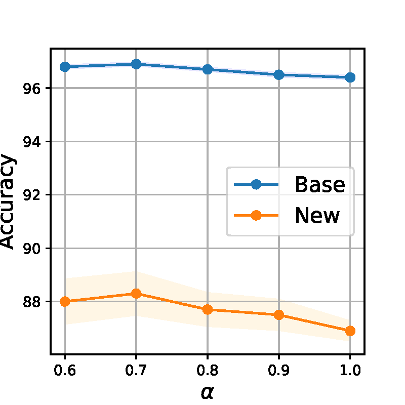
(a) Oxford Pets

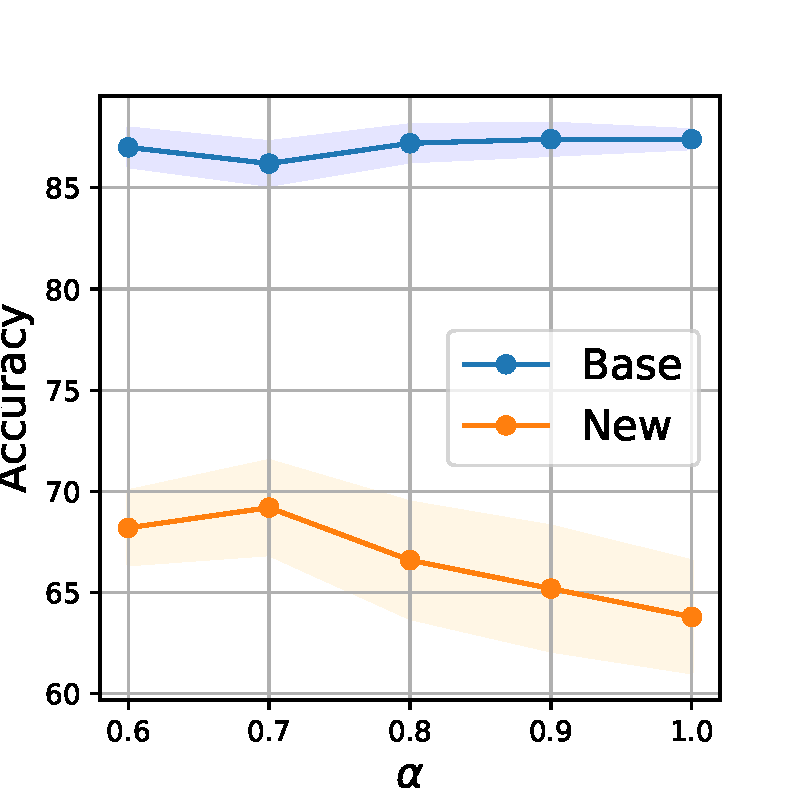
(b) UCF101

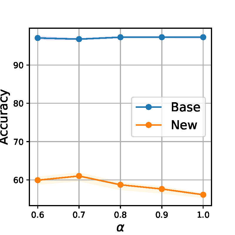
(c) Flower102

Figure 4: Sensitivity analysis on $\alpha$, effect of test data-dependent prior. Experiments are replicated over 3 times.

Domain Generalization on ImageNet

Despite the tendency for a potential performance trade-off between the source and target datasets, table 6 demonstrates APP attains the improved performance achieved on both the source and target datasets, highlighting the robustness of APP in dealing with distribution shifts.

Table 6: Result of domain generalization in ImageNet. Acc represents the accuracy. Bold means the best accuracy.

	Dataset	Methods	Acc ($\%$)
Source	ImageNet	CoCoOp	$63.13\pm 0.12$
		PLOT	$63.14\pm 0.16$
		ProDA	$62.73\pm 0.11$
		APP	$\mathbf{64.50\pm 0.06}$
Target	ImageNetV2	CoCoOp	$55.23\pm 0.25$
		PLOT	$54.23\pm 0.45$
		ProDA	$54.97\pm 0.05$
		APP	$\mathbf{57.10\pm 0.29}$
	ImageNet-Sketch	CoCoOp	$34.07\pm 0.46$
		PLOT	$33.93\pm 0.12$
		ProDA	$34.60\pm 0.22$
		APP	$\mathbf{35.70\pm 0.14}$
	ImageNet-R	CoCoOp	$56.03\pm 0.38$
		PLOT	$56.86\pm 0.42$
		ProDA	$58.57\pm 0.49$
		APP	$\mathbf{58.70\pm 0.08}$
	ImageNet-A	CoCoOp	$22.37\pm 0.09$
		PLOT	$22.63\pm 0.12$
		ProDA	$23.47\pm 0.12$
		APP	$\mathbf{23.80\pm 0.22}$

Conclusion

We propose the Bayesian framework for prompt learning to consider the uncertainty from few-shot learning scenario, where the image features are possible to be multi-modal and a distribution shift exists between the train and test dataset. We enhance flexibility via Wasserstein Gradient Flow. Furthermore, we propose a novel data-dependent prior distribution that is conditioned on averaged image features. This approach is designed to capture minor modes of image features and facilitate adaptation to previously unseen distributions. We demonstrate substantial performance improvements in various scenarios, including few-shot classifications, domain generalizations, and unseen class generalizations. Additionally, the qualitative analyses indicate that our prompt learning facilitates capturing the multi-modes of image features sparsely.

Supplementary Material

Proof of Proposition 1

For simplicity, define the $A\coloneqq f(X)$ and $B\coloneqq g(\phi(f(X)),\cdot)$. Following (Barber and Agakov 2003), we formulate the variational bound for Mutual information as follows:

$$I\left(f(X);g(\phi(f(X)),\cdot)\right)\coloneqq I(A;B)=\operatorname{\mathbb{E}}_{p(A,B)}\log{p(B|A)\over p(B)}\geq E_{p(A,B)}\log{q(B|A)\over p(B)}$$ (17)

where $q$ is a variational distribution. Following (Sordoni et al. 2021), we define variational distribution $q$ by sampling $B_{1},...,B_{C}$ from the distribution $p(B)$, where $B_{i}\coloneqq g(\phi(f(X)),y_{i})$. For formulating the variational distribution, we choose the $B_{i}$ by the importance weight, which is defined as ${\exp(sim(A,B_{j})/\tau)\over\sum_{i=1}^{C}\exp((sim(A,B_{i}))/\tau)}$.

Therefore, unnormalized variational distribution for $B_{1}$ is defined as follows:

$$q(B_{1}|A,B_{2:C})=p(B_{1}){C\cdot\exp(sim(A,B_{1})/\tau)\over\sum_{i=1}^{C}\exp((sim(A,B_{i}))/\tau)}$$ (18)

By Jensen’s inequality, the lower bound of Eq. 17 is derived as follows:

$$\operatorname{\mathbb{E}}_{p(A,B_{1})}\log\operatorname{\mathbb{E}}_{p(B_{2:C})}\left({q(B_{1}|A,B_{2:C})\over p(B_{1})}\right) \geq\operatorname{\mathbb{E}}_{p(A,B_{1})p(B_{2:C})}\log\left({p(B_{1}){C\cdot\exp(sim(A,B_{1})/\tau)\over\sum_{i=1}^{C}\exp((sim(A,B_{i}))/\tau)}\over p(B_{1})}\right)$$

$$=\operatorname{\mathbb{E}}_{p(A,B_{1})p(B_{2:C})}\log\left({{C\cdot\exp(sim(A,B_{1})/\tau)\over\sum_{i=1}^{C}\exp((sim(A,B_{i}))/\tau)}}\right)$$

$$=\log C-\mathcal{L}_{CE}(\phi(f(X)),X,Y)$$ (19)

For training the prior network, we minimize the $\mathcal{L}_{CE}$, which is the upper bound of Mutual information.

Derivation from Wasserstein Gradient Flow to Stein Variational Gradient Descent

Define the functional $F$ as follows:

$$F(\mu)\coloneqq D_{KL}(\mu||\pi)$$ (20)

, where $\pi\propto\exp(-V(\theta))$. Then, Wasserstein Gradient is defined as follows:

$$\nabla{\delta F(\mu)\over\delta\mu}=\nabla\log{\mu\over\pi}$$ (21)

Considering Wasserstein Gradient in RKHS with transformation $\mathcal{K}_{\mu}T(\theta)\coloneqq\operatorname{\mathbb{E}}_{\theta^{\prime}\sim\mu}[K({\theta},{\theta^{\prime}})T({\theta^{\prime}})]$, we derive kernelized Wasserstein Gradient as follows:

$$\mathcal{K}_{\mu}\nabla_{\theta^{\prime}}{\delta F(\mu)\over\delta\mu} =\mathcal{K}_{\mu}\nabla_{\theta^{\prime}}\log{\mu\over\pi}$$ (22)

$$=\int K({\theta},{\theta^{\prime}})(-\nabla_{\theta^{\prime}}\log\pi+\nabla_{\theta^{\prime}}\log\mu)\mu(\theta^{\prime})d\theta^{\prime}$$ (23)

$$=\int K({\theta},{\theta^{\prime}})(\nabla_{\theta^{\prime}}V(\theta^{\prime})+\nabla_{\theta^{\prime}}\log\mu)\mu(\theta^{\prime})d\theta^{\prime}$$ (24)

$$=\int K({\theta},{\theta^{\prime}})\nabla_{\theta^{\prime}}V(\theta^{\prime})\mu d\theta^{\prime}-\int\nabla_{\theta^{\prime}}K({\theta},{\theta^{\prime}})\mu d\theta^{\prime}+\underbrace{[K({\theta},{\theta^{\prime}})\mu]\big{|}_{\|\theta^{\prime}\|\rightarrow\infty}}_{=0}$$ (25)

By the Continuity equation, evolving path of $\theta$ is derived as follows:

$$\partial_{t}\theta_{t} =-\mathcal{K}_{\mu}\nabla_{\theta^{\prime}}({\delta F(\mu)\over\delta\mu})$$

$$=-[\int K({\theta},{\theta^{\prime}})\nabla_{\theta^{\prime}}V(\theta^{\prime})\mu d\theta^{\prime}-\int\nabla_{\theta^{\prime}}K({\theta},{\theta^{\prime}})\mu d\theta^{\prime}]$$ (26)

By discretization, we formulate the following update rule:

$$\theta_{t+1}^{i}=\theta_{t}^{i}-{h\over M}\sum_{j=1}^{M}[K(\theta_{t}^{i},\theta_{t}^{j})\nabla_{\theta_{t}^{j}}V(\theta_{t}^{j})-\nabla_{\theta_{t}^{j}}K(\theta_{t}^{i},\theta_{t}^{j})]$$ (27)

Implementation Details

We adopted the training settings from the work of (Chen et al. 2023). In our experiments, we used a batch size of 32 for the Oxford-Flowers, FGVC-Aircraft, and Stanford-Cars datasets, while the batch size for other datasets was fixed at 128. The prior network was trained for 10, 20, 20, 40, and 40 shots for each respective dataset. We employed the SGD optimizer with an initial learning rate of 0.002, which was annealed using the CosineAnnealing schedule. All experiments were conducted on a single NVIDIA A100 GPU core.

For evaluation, we considered the model output within a Bayesian framework, taking into account the posterior distribution $p(\theta|X,Y)$. Thus, predictive distribution for test data point $x^{\prime}$ is defined as follows:

$$p(y^{\prime}|x^{\prime},\mathcal{D})=\int p(y^{\prime}|x^{\prime},\theta)p(\theta|\mathcal{D},x^{\prime})d\theta$$ (28)

, where $\mathcal{D}\coloneqq\{X,Y\}$

Table 7 indicates a performance comparison between ours and other multi-prompts methods.

Table 7: Result of Few-shot Classification. We report the mean accuracy by conducting three-replicated experiments.

Dataset	Methods	1 shot	2 shots	4 shots	8 shots	16 shots
Caltech101	PLOT (Chen et al. 2023)	$89.72\pm 0.44$	$90.48\pm 0.22$	$90.99\pm 0.30$	$91.23\pm 0.46$	$92.29\pm 0.22$
	ProDA (Lu et al. 2022)	$89.14\pm 0.19$	$90.08\pm 0.50$	$90.94\pm 0.19$	$91.83\pm 0.27$	$92.47\pm 0.08$
	Ours	$\mathbf{90.30\pm 0.33}$	$\mathbf{90.87\pm 0.25}$	$\mathbf{91.05\pm 0.45}$	$\mathbf{91.92\pm 0.08}$	$\mathbf{92.89\pm 0.22}$
DTD	PLOT (Chen et al. 2023)	$46.94\pm 1.89$	$51.46\pm 2.27$	$55.95\pm 0.74$	$61.68\pm 0.34$	$65.27\pm 0.23$
	ProDA (Lu et al. 2022)	$47.52\pm 1.69$	$\mathbf{52.17\pm 1.89}$	$55.85\pm 0.92$	$62.74\pm 0.38$	$66.27\pm 1.11$
	Ours	$\mathbf{49.09\pm 2.29}$	$51.73\pm 3.47$	$\mathbf{58.06\pm 0.69}$	$\mathbf{63.42\pm 0.12}$	$\mathbf{66.57\pm 0.07}$
EuroSAT	PLOT (Chen et al. 2023)	$54.15\pm 2.04$	$63.64\pm 3.08$	$74.91\pm 2.13$	$78.55\pm 1.33$	$84.06\pm 0.91$
	ProDA (Lu et al. 2022)	$49.89\pm 2.37$	$62.37\pm 1.41$	$70.38\pm 1.73$	$77.20\pm 1.97$	$80.62\pm 1.51$
	Ours	$\mathbf{60.04\pm 2.08}$	$\mathbf{66.02\pm 2.70}$	$\mathbf{74.08\pm 2.23}$	$\mathbf{77.87\pm 2.51}$	$\mathbf{84.08\pm 1.1}$
FGVC-Aircraft	PLOT (Chen et al. 2023)	$18.22\pm 0.59$	$19.26\pm 0.96$	$22.39\pm 1.41$	$27.58\pm 0.83$	$32.28\pm 0.43$
	ProDA (Lu et al. 2022)	$\mathbf{20.25\pm 0.88}$	$\mathbf{22.45\pm 0.37}$	$24.76\pm 1.00$	$28.46\pm 0.43$	$32.84\pm 0.34$
	Ours	$18.10\pm 0.92$	$21.87\pm 1.21$	$\mathbf{25.65\pm 0.59}$	$\mathbf{29.40\pm 0.42}$	$\mathbf{33.80\pm 0.53}$
Food101	PLOT (Chen et al. 2023)	$77.87\pm 0.13$	$77.78\pm 0.37$	$77.20\pm 0.37$	$75.42\pm 0.09$	$77.18\pm 0.16$
	ProDA (Lu et al. 2022)	$78.65\pm 0.17$	$79.04\pm 0.17$	$\mathbf{79.47\pm 0.17}$	$78.88\pm 0.22$	$79.82\pm 0.10$
	Ours	$\mathbf{78.87\pm 0.17}$	$\mathbf{79.25\pm 0.06}$	$79.43\pm 0.10$	$\mathbf{79.49\pm 0.17}$	$\mathbf{79.83\pm 0.06}$
ImageNet	PLOT (Chen et al. 2023)	$59.32\pm 0.58$	$59.81\pm 0.25$	$61.12\pm 0.14$	$61.91\pm 0.09$	$63.14\pm 0.16$
	ProDA (Lu et al. 2022)	$61.65\pm 0.46$	$62.20\pm 0.11$	$61.96\pm 0.30$	$61.78\pm 0.29$	$62.73\pm 0.11$
	Ours	$\mathbf{62.11\pm 0.26}$	$\mathbf{62.50\pm 0.10}$	$\mathbf{63.05\pm 0.15}$	$\mathbf{63.70\pm 0.17}$	$\mathbf{64.50\pm 0.06}$
Oxford Flowers	PLOT (Chen et al. 2023)	$72.32\pm 0.94$	$82.65\pm 0.38$	$88.13\pm 0.27$	$92.56\pm 0.02$	$95.64\pm 0.28$
	ProDA (Lu et al. 2022)	$70.56\pm 0.48$	$83.73\pm 0.50$	$88.94\pm 0.30$	$93.30\pm 0.35$	$95.47\pm 0.18$
	Ours	$\mathbf{74.42\pm 0.58}$	$\mathbf{84.23\pm 0.14}$	$\mathbf{89.13\pm 0.31}$	$\mathbf{93.38\pm 0.09}$	$\mathbf{95.67\pm 0.09}$
Oxford Pets	PLOT (Chen et al. 2023)	$87.35\pm 0.67$	$87.16\pm 0.37$	$88.25\pm 0.58$	$87.39\pm 0.39$	$87.20\pm 0.20$
	ProDA (Lu et al. 2022)	$88.76\pm 0.08$	$88.15\pm 0.39$	$89.17\pm 0.41$	$\mathbf{89.97\pm 0.23}$	$89.61\pm 0.36$
	Ours	$\mathbf{88.97\pm 0.52}$	$\mathbf{88.28\pm 0.39}$	$\mathbf{89.48\pm 0.28}$	$89.79\pm 0.16$	$\mathbf{89.73\pm 0.63}$
Stanford Cars	PLOT (Chen et al. 2023)	$56.21\pm 0.78$	$57.35\pm 0.27$	$63.35\pm 0.54$	$67.60\pm 0.05$	$73.78\pm 0.11$
	ProDA (Lu et al. 2022)	$59.55\pm 0.13$	$62.08\pm 0.65$	$66.32\pm 0.18$	$71.11\pm 0.21$	$74.86\pm 0.21$
	Ours	$\mathbf{59.65\pm 0.41}$	$\mathbf{63.39\pm 0.35}$	$\mathbf{67.18\pm 0.30}$	$\mathbf{71.86\pm 0.11}$	$\mathbf{76.14\pm 0.23}$
Sun397	PLOT (Chen et al. 2023)	$63.03\pm 0.32$	$62.10\pm 0.50$	$65.60\pm 0.44$	$66.90\pm 0.25$	$69.76\pm 0.29$
	ProDA (Lu et al. 2022)	$\mathbf{63.99\pm 0.15}$	$65.56\pm 0.40$	$\mathbf{67.79\pm 0.49}$	$\mathbf{69.50\pm 0.13}$	$\mathbf{71.61\pm 0.18}$
	Ours	$\mathbf{63.99\pm 0.20}$	$\mathbf{65.59\pm 0.19}$	$67.01\pm 0.36$	$69.46\pm 0.08$	$71.59\pm 0.19$
UCF101	PLOT (Chen et al. 2023)	$64.31\pm 0.36$	$67.64\pm 0.42$	$70.87\pm 0.32$	$75.77\pm 0.25$	$77.58\pm 0.29$
	ProDA (Lu et al. 2022)	$64.44\pm 0.68$	$67.80\pm 0.11$	$70.78\pm 0.23$	$\mathbf{77.01\pm 0.35}$	$\mathbf{79.34\pm 0.68}$
	Ours	$\mathbf{65.83\pm 0.84}$	$\mathbf{69.05\pm 0.19}$	$\mathbf{71.79\pm 0.13}$	$76.71\pm 0.60$	$79.07\pm 0.12$
Average	PLOT (Chen et al. 2023)	$62.68\pm 0.09$	$65.39\pm 0.48$	$68.98\pm 0.24$	$71.51\pm 0.10$	$74.38\pm 0.06$
	ProDA (Lu et al. 2022)	$63.13\pm 0.26$	$66.88\pm 0.22$	$69.67\pm 0.16$	$72.89\pm 0.25$	$75.06\pm 0.05$
	Ours	$\mathbf{64.67\pm 0.26}$	$\mathbf{67.53\pm 0.50}$	$\mathbf{70.54\pm 0.15}$	$\mathbf{73.36\pm 0.24}$	$\mathbf{75.81\pm 0.06}$

Semantics of Prompts

To analyze the semantic meaning of the learned context vectors in our approach, we performed a study where we extracted the nearest words in the embedding space of each context vector. While not all vectors have a straightforward semantic interpretation in continuous space, we observed that certain components of each context vector exhibited clear semantic relevance and effectively described the image data.

Table 8 demonstrates that each context vector is trained in a direction that corresponds to specific aspects of the image data. This finding indicates that our model has successfully learned to capture meaningful representations of the image content within the context vectors. For instance, context 1 contains words such as ”americanair” and ”usnavy,” which are associated with civil aircraft and fighter aircraft, respectively, in the dataset.

Table 8: Interpretable and closest words to our context vectors for FGVC-Aircraft. We report one of the top 4 words, which are interpretable. - means that there are no interpretable words and bold means highly relevant words to datasets.

Number	Context 1	Context 2	Context 3	Context 4
1	sculpt	calling	salazar	-
2	espn	byte	grassroots	bucketlist
3	postponed	turquoise	installation	below
4	grocery	wig	followed	accepted
5	taking	shells	translates	turkish
6	usnavy	likes	administrator	fair
7	fort	-	centred	qantas
8	staten	fo	blaze	modern
9	rusher	tue	attempting	serve
10	wielding	ata	-	crossing
11	trick	brown	blowing	-
12	pate	vfl	donkey	occasion
13	americanair	-	legendary	times
14	eight	ima	reunite	inevit
15	..?	thanku	flew	letting
16	brox	facing	!	grand

Empirical comparison with BPL

Table 9 (unseen classes generalization experiments) indicates that APP is more efficient in time and memory complexity with more robust performance, harmonic mean (accuracies between base and new classes). This gain demonstrates that the Gaussian variational distribution of BPL is not sufficient to capture the whole multimodes of image features. In addition, the conditional posterior assumption is not scalable, when the batch size is set to high.

Dataset	Method	BS	Memory (GB)	Time (hr)	H (%)
Caltech101	BPL	1	11.0	5.75	$92.3$
		128	-	-	-
	APP (Ours)	1	$\mathbf{10.6}$	$\mathbf{2.50}$	$\mathbf{93.0}$
		128	$\mathbf{10.8}$	$\mathbf{0.25}$	$\mathbf{93.0}$
Oxford pets	BPL	1	7.4	1.5	$91.5$
		128	-	-	-
	APP (Ours)	1	$\mathbf{7.0}$	$\mathbf{0.83}$	$\mathbf{91.7}$
		128	$\mathbf{8.2}$	$\mathbf{0.06}$	$\mathbf{92.4}$
UCF101	BPL	1	11.5	9.26	$72.8$
		128	-	-	-
	APP (Ours)	1	$\mathbf{7.0}$	$\mathbf{3.25}$	$\mathbf{73.3}$
		128	$\mathbf{8.5}$	$\mathbf{0.1}$	$\mathbf{76.8}$

Table 9: Results of BPL in unseen classes generalization experiments. We report the performance of three replicated experiments. The symbol ”-” indicates the training failure due to the memory issue.

References

- Barber and Agakov (2003) Barber, D.; and Agakov, F. 2003. Information Maximization in Noisy Channels : A Variational Approach. In Thrun, S.; Saul, L.; and Schölkopf, B., eds., Advances in Neural Information Processing Systems, volume 16. MIT Press.
- Beaudry and Renner (2012) Beaudry, N. J.; and Renner, R. 2012. An intuitive proof of the data processing inequality. arXiv:1107.0740.
- Bossard, Guillaumin, and Van Gool (2014) Bossard, L.; Guillaumin, M.; and Van Gool, L. 2014. Food-101–mining discriminative components with random forests. In Computer Vision–ECCV 2014: 13th European Conference, Zurich, Switzerland, September 6-12, 2014, Proceedings, Part VI 13, 446–461. Springer.
- Chen et al. (2018) Chen, C.; Zhang, R.; Wang, W.; Li, B.; and Chen, L. 2018. A Unified Particle-Optimization Framework for Scalable Bayesian Sampling. arXiv:1805.11659.
- Chen et al. (2023) Chen, G.; Yao, W.; Song, X.; Li, X.; Rao, Y.; and Zhang, K. 2023. PLOT: Prompt Learning with Optimal Transport for Vision-Language Models. In The Eleventh International Conference on Learning Representations.
- Cimpoi et al. (2014) Cimpoi, M.; Maji, S.; Kokkinos, I.; Mohamed, S.; and Vedaldi, A. 2014. Describing textures in the wild. In Proceedings of the IEEE conference on computer vision and pattern recognition, 3606–3613.
- Deng et al. (2009) Deng, J.; Dong, W.; Socher, R.; Li, L.-J.; Li, K.; and Fei-Fei, L. 2009. Imagenet: A large-scale hierarchical image database. In 2009 IEEE conference on computer vision and pattern recognition, 248–255. Ieee.
- Derakhshani et al. (2023) Derakhshani, M. M.; Sanchez, E.; Bulat, A.; da Costa, V. G. T.; Snoek, C. G. M.; Tzimiropoulos, G.; and Martinez, B. 2023. Bayesian Prompt Learning for Image-Language Model Generalization. arXiv:2210.02390.
- Fei-Fei, Fergus, and Perona (2004) Fei-Fei, L.; Fergus, R.; and Perona, P. 2004. Learning generative visual models from few training examples: An incremental bayesian approach tested on 101 object categories. In 2004 conference on computer vision and pattern recognition workshop, 178–178. IEEE.
- gil Lee et al. (2022) gil Lee, S.; Kim, H.; Shin, C.; Tan, X.; Liu, C.; Meng, Q.; Qin, T.; Chen, W.; Yoon, S.; and Liu, T.-Y. 2022. PriorGrad: Improving Conditional Denoising Diffusion Models with Data-Dependent Adaptive Prior. In International Conference on Learning Representations.
- He et al. (2016) He, K.; Zhang, X.; Ren, S.; and Sun, J. 2016. Deep residual learning for image recognition. In Proceedings of the IEEE conference on computer vision and pattern recognition, 770–778.
- Helber et al. (2019) Helber, P.; Bischke, B.; Dengel, A.; and Borth, D. 2019. Eurosat: A novel dataset and deep learning benchmark for land use and land cover classification. IEEE Journal of Selected Topics in Applied Earth Observations and Remote Sensing, 12(7): 2217–2226.
- Hendrycks et al. (2021a) Hendrycks, D.; Basart, S.; Mu, N.; Kadavath, S.; Wang, F.; Dorundo, E.; Desai, R.; Zhu, T.; Parajuli, S.; Guo, M.; et al. 2021a. The many faces of robustness: A critical analysis of out-of-distribution generalization. In Proceedings of the IEEE/CVF International Conference on Computer Vision, 8340–8349.
- Hendrycks et al. (2021b) Hendrycks, D.; Zhao, K.; Basart, S.; Steinhardt, J.; and Song, D. 2021b. Natural adversarial examples. In Proceedings of the IEEE/CVF Conference on Computer Vision and Pattern Recognition, 15262–15271.
- Jia et al. (2021) Jia, C.; Yang, Y.; Xia, Y.; Chen, Y.-T.; Parekh, Z.; Pham, H.; Le, Q.; Sung, Y.-H.; Li, Z.; and Duerig, T. 2021. Scaling up visual and vision-language representation learning with noisy text supervision. In International Conference on Machine Learning, 4904–4916. PMLR.
- Jordan, Kinderlehrer, and Otto (1998) Jordan, R.; Kinderlehrer, D.; and Otto, F. 1998. The Variational Formulation of the Fokker–Planck Equation. SIAM Journal on Mathematical Analysis, 29(1): 1–17.
- Krause et al. (2013) Krause, J.; Stark, M.; Deng, J.; and Fei-Fei, L. 2013. 3d object representations for fine-grained categorization. In Proceedings of the IEEE international conference on computer vision workshops, 554–561.
- Li et al. (2020) Li, Z.; Wang, R.; Chen, K.; Utiyama, M.; Sumita, E.; Zhang, Z.; and Zhao, H. 2020. Data-dependent Gaussian Prior Objective for Language Generation. In International Conference on Learning Representations.
- Liu and Wang (2016) Liu, Q.; and Wang, D. 2016. Stein Variational Gradient Descent: A General Purpose Bayesian Inference Algorithm. In Lee, D.; Sugiyama, M.; Luxburg, U.; Guyon, I.; and Garnett, R., eds., Advances in Neural Information Processing Systems, volume 29. Curran Associates, Inc.
- Lu et al. (2022) Lu, Y.; Liu, J.; Zhang, Y.; Liu, Y.; and Tian, X. 2022. Prompt distribution learning. In Proceedings of the IEEE/CVF Conference on Computer Vision and Pattern Recognition, 5206–5215.
- Maji et al. (2013) Maji, S.; Rahtu, E.; Kannala, J.; Blaschko, M.; and Vedaldi, A. 2013. Fine-grained visual classification of aircraft. arXiv preprint arXiv:1306.5151.
- McInnes, Healy, and Melville (2018) McInnes, L.; Healy, J.; and Melville, J. 2018. Umap: Uniform manifold approximation and projection for dimension reduction. arXiv preprint arXiv:1802.03426.
- Nilsback and Zisserman (2008) Nilsback, M.-E.; and Zisserman, A. 2008. Automated flower classification over a large number of classes. In 2008 Sixth Indian Conference on Computer Vision, Graphics & Image Processing, 722–729. IEEE.
- Parkhi et al. (2012) Parkhi, O. M.; Vedaldi, A.; Zisserman, A.; and Jawahar, C. V. 2012. Cats and dogs. In 2012 IEEE Conference on Computer Vision and Pattern Recognition, 3498–3505.
- Radford et al. (2021) Radford, A.; Kim, J. W.; Hallacy, C.; Ramesh, A.; Goh, G.; Agarwal, S.; Sastry, G.; Askell, A.; Mishkin, P.; Clark, J.; et al. 2021. Learning transferable visual models from natural language supervision. In International conference on machine learning, 8748–8763. PMLR.
- Recht et al. (2019) Recht, B.; Roelofs, R.; Schmidt, L.; and Shankar, V. 2019. Do imagenet classifiers generalize to imagenet? In International conference on machine learning, 5389–5400. PMLR.
- Ruan, Dubois, and Maddison (2022) Ruan, Y.; Dubois, Y.; and Maddison, C. J. 2022. Optimal Representations for Covariate Shift. In International Conference on Learning Representations.
- Shen et al. (2022) Shen, S.; Li, L. H.; Tan, H.; Bansal, M.; Rohrbach, A.; Chang, K.-W.; Yao, Z.; and Keutzer, K. 2022. How Much Can CLIP Benefit Vision-and-Language Tasks? In International Conference on Learning Representations.
- Soomro, Zamir, and Shah (2012) Soomro, K.; Zamir, A. R.; and Shah, M. 2012. UCF101: A dataset of 101 human actions classes from videos in the wild. arXiv preprint arXiv:1212.0402.
- Sordoni et al. (2021) Sordoni, A.; Dziri, N.; Schulz, H.; Gordon, G.; Bachman, P.; and Des Combes, R. T. 2021. Decomposed mutual information estimation for contrastive representation learning. In International Conference on Machine Learning, 9859–9869. PMLR.
- Wang et al. (2019) Wang, H.; Ge, S.; Lipton, Z.; and Xing, E. P. 2019. Learning robust global representations by penalizing local predictive power. Advances in Neural Information Processing Systems, 32.
- Welling and Teh (2011) Welling, M.; and Teh, Y. W. 2011. Bayesian learning via stochastic gradient Langevin dynamics. In Proceedings of the 28th international conference on machine learning (ICML-11), 681–688.
- Wortsman et al. (2022) Wortsman, M.; Ilharco, G.; Kim, J. W.; Li, M.; Kornblith, S.; Roelofs, R.; Lopes, R. G.; Hajishirzi, H.; Farhadi, A.; Namkoong, H.; et al. 2022. Robust fine-tuning of zero-shot models. In Proceedings of the IEEE/CVF Conference on Computer Vision and Pattern Recognition, 7959–7971.
- Xiao et al. (2010) Xiao, J.; Hays, J.; Ehinger, K. A.; Oliva, A.; and Torralba, A. 2010. Sun database: Large-scale scene recognition from abbey to zoo. In 2010 IEEE computer society conference on computer vision and pattern recognition, 3485–3492. IEEE.
- Zhou et al. (2022a) Zhou, K.; Yang, J.; Loy, C. C.; and Liu, Z. 2022a. Conditional prompt learning for vision-language models. In Proceedings of the IEEE/CVF Conference on Computer Vision and Pattern Recognition, 16816–16825.
- Zhou et al. (2022b) Zhou, K.; Yang, J.; Loy, C. C.; and Liu, Z. 2022b. Learning to prompt for vision-language models. International Journal of Computer Vision, 130(9): 2337–2348.