labelinglabel
Energy-Efficient Data Offloading for
Earth Observation Satellite Networks
Abstract
In Earth Observation Satellite Networks (EOSNs) with a large number of battery-carrying satellites, proper power allocation and task scheduling are crucial to improving the data offloading efficiency. As such, we jointly optimize power allocation and task scheduling to achieve energy-efficient data offloading in EOSNs, aiming to balance the objectives of reducing the total energy consumption and increasing the sum weights of tasks. First, we derive the optimal power allocation solution to the joint optimization problem when the task scheduling policy is given. Second, leveraging the conflict graph model, we transform the original joint optimization problem into a maximum weight independent set problem when the power allocation strategy is given. Finally, we utilize the genetic framework to combine the above special solutions as a two-layer solution for the joint optimization problem. Simulation results demonstrate that our proposed solution can properly balance the sum weights of tasks and the total energy consumption, achieving superior system performance over the current best alternatives.
I Introduction
Driven by the fast proliferation of remote sensing applications, such as environment monitoring, meteorology, and natural disaster surveillance, Earth Observation Satellite Networks (EOSNs) experience an explosive growth in remote sensing data [1, 2, 3]. There arises an urgent need to offload the collected remote sensing data from EOSNs to Ground Stations (GSs) for further data processing. Different from traditional ground wireless networks, EOSNs belong to Ad Hoc networks with dynamic network topologies [4]. This means that data offloading in EOSNs occurs only within limited Transmission Time Windows (TTWs) between Earth Observation Satellites (EOSs) and GSs due to the high-speed motion of EOSs. The key to efficient data offloading in EOSNs is how to schedule data offloading tasks within limited TTWs to maximize the desired network performance[5].
From the mathematical perspective, the data offloading problem in EOSNs is similar to the Parallel Machine Scheduling Problem with Time Windows (PMSPTW)[6]. Recently, a majority of works studied the PMSPTW to select a set of optimal GSs for Low Earth Orbit (LEO) satellites to schedule Satellite Ground Links (SGLs) while satisfying the time window constraints [7, 8, 9, 10, 11, 12, 13]. The scheduling algorithms proposed in these works are either deterministic [7, 8] or non-deterministic[9, 10, 11, 12, 13]. The deterministic algorithms use mathematical tools, such as tree search[7] and dynamic programming[8], to find an optimal solution under mild assumptions. However, these deterministic algorithms are time-consuming especially for large-scale problems and thus are not suitable for practical EOSNs. To accommodate large-scale EOSNs, some non-deterministic algorithms have been proposed to find approximation solutions with lower computation costs. They are mainly based on meta-heuristic methods, such as particle swarm optimization[9], ant colony optimization[10], and genetic algorithm [11]. Recently, some attempts have been made to utilize Deep Reinforcement Learning (DRL) for solving satellite scheduling problems. For example, the PMSPTW was transformed into an Assignment Problem (AP) and a Single Antenna Scheduling Problem (SASP) [12]. Then, the DRL method and a heuristic scheduling method were proposed to solve the AP and the SASP, respectively. In [13], a DRL-based algorithm was proposed for a rapid satellite range rescheduling problem to process real-time emergency events.
However, the above works ignored the energy management of battery-carrying LEO satellites powered by the solar panels, resulting in data offloading interruptions due to the overuse of energy. As such, energy consumption control is crucial for efficient data offloading in EOSNs[14]. To improve data offloading efficiency, some researchers studied energy-efficient offloading for various satellite networks, such as land mobile satellite systems[15], cognitive satellite terrestrial networks[16], small satellite cluster networks [17], and satellite-terrestrial networks [18]. In these works, each offloading task is represented as a set of equal packets, and then energy-efficient scheduling strategies are proposed to download these packets. In this case, the decision variables for scheduling packets form a huge solution space, increasing the difficulty of solving the problem. Therefore, these works [15, 16, 18, 17] are unsuitable for EOSNs to offload the tasks with a large amount of data.
In contrast to previous works [15, 16, 18, 17], in this work, we character the main features of data offloading in real EOSNs from the following three aspects. First, we consider a more realistic data offloading scenario with variable-size tasks. Second, our proposed joint optimization framework incorporates the time window constraints of data offloading in EOSNs, which captures the intermittent characteristic of SGLs. Third, we develop an efficient yet fast two-layer optimization solution, termed Energy-efficient Data Offloading (EDO), to minimize the total energy consumption while maximizing the sum weights of tasks.
II System Model and Problem Formulation
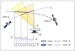
We consider a downlink EOSN consisting of a set of EOSs and a set of GSs. We discretize the whole scheduling horizon into time slots to obtain a set of time slots, denoted by . We denote by time slot the time interval of . We assume that each EOS and each GS is respectively equipped with one transmit antenna and one receiver antenna. Let denote the set of data receiver antennas. As shown in Fig. 1, EOSs cycle their individual orbits at high speed, thereby yielding a set of short contact TTWs. Let denote the set of TTWs between each EOS and each antenna . Let . We use 4-tuples to represent each TTW , where and are the beginning and end times, respectively. We denote by the set of data offloading tasks. Let index the EOS that stores the data of task .
II-A Channel Model
We denote by the achievable data rate of SGLs within TTW in bits/s for any task , given by
| (1) |
where is the bandwidth and is the signal-to-noise ratio of offloading task within TTW . We evaluate the of SGLs [19] as follows:
| (2) |
where represents the transmit antenna gain of EOS , denotes the gain of receiver antenna , is the free space loss, is the noise power, and is the total path loss for TTW . The total path loss in dB is calculated by , where denotes the basic path loss in dB, represents the attenuation due to atmospheric gasses in dB, indicates the attenuation due to either ionospheric or tropospheric scintillation in dB, and is the building entry loss in dB for TTW [20]. In particular, represents the transmit power of EOS allocated to task , which is subject to the following transmit power range of each EOS:
| (3) |
Furthermore, we let represent the rate requirement of TTW and introduce the following constraint to indicate the rate requirement of each TTW:
| (4) |
II-B Task Model
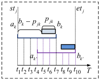
Let and denote the data amount of task and the weighted value of task , respectively. We denote by the processing time, i.e., the transmitting time, of task within TTW , which can be computed by
| (5) |
Let and be the earliest time and the latest time to start offloading task , respectively. We use 6-tuples to represent each task . Furthermore, we use a decision variable to represent the offloading strategy, such that indicates that the data of task is offloaded in time slot within TTW ; and otherwise. Thus, we introduce the following binary constraint
| (6) |
to indicate whether task starts to offload in time slot within TTW , or not. Wherein, represents the set of all feasible time slots for task , given by
| (7) |
with indicating the set of feasible slots within TTW to start offloading the data of task . As an example for illustration in Fig. 2, we have .
We further introduce the following constraint to guarantee that each task is offloaded at most once:
| (8) |
In addition, we denote by the energy consumption for offloading task , which is calculated by
| (9) |
II-C Time Window Model
We define the set of occupying time slots for antenna to receive the data of task in time slot as
We can see from the example in Fig. 2 that . As such, the following constraint reveals that any receiver antenna receives the data of at most one task in any time slot:
| (10) |
Similarly, we define the set of occupying feasible time slots for EOS to offload the data of task in time slot as follows:
We further use the following constraint to indicate that any EOS offloads the data of at most one task in any time slot:
| (11) |
II-D Problem Formulation
To balance the two conflicting objectives of minimizing the total energy consumption and maximizing the sum weights of tasks, we consider their normalized weighted sum and formulate the following mixed integer programming problem:
| (12) |
where , , denotes the sum weights of all the tasks, represents the sum of the maximization energy consumption of all tasks, and is a tuning weighted coefficient to obtain the desired total energy consumption and sum weights of tasks. Note that the distinct characteristic of the data offloading in EOSNs is mainly reflected in the time window constraints of C5 and C6.
III Proposed Solution
In this section, we first study two cases for to obtain two special solutions and then utilize the genetic framework to combine them as an efficient two-layer solution.
III-A Power Allocation for Fixed Task Scheduling
With a given task scheduling decision , degrades into the total energy consumption minimization problem:
where is a constant, given by
| (13) |
We further explore the unique structure of to obtain the optimal power allocation solution. We observe that can be decomposed into independent subproblems and one for each task , given by
In line with (1) and (2), we obtain
| (14) |
Combining (5) and (9), we have
| (15) |
We combine (III-A) with (15) to obtain:
| (16) |
where and . To study the properties of , we first introduce a new variable with each element satisfying
| (17) |
We further use to recast as the following new form:
where and . Next, we can obtain the first-order and second-order derivation of as follows:
| (18) | |||
| (19) |
For any subject to , we have , which indicates that is a convex and unimodal function. Thus, the optimal solution to is either , , or the extreme point of , depending on the value of , given by
| (23) |
where satisfies . In particular, we can use the bisection method to obtain . Therefore, we obtain the optimal solution to :
| (24) |
III-B Task Scheduling for Fixed Power Allocation
With a given power allocation solution , degrades into the following task scheduling problem:
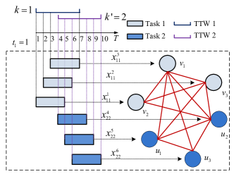
To solve efficiently, we leverage a conflict graph model with and respectively representing the vertex set and edge set, to depict the conflict relations among variables. We take the following two steps to construct conflict graph . First, we construct vertex set by representing any variable as a vertex one by one. As such, we establish one to one mapping between and . Second, from the constraints of , we can check whether any two variables (denoted by ) and (denoted by ) take the value of one at the same time. If not, we can add one edge across the vertexes and . We perform this procedure on all combinations on to constitute vertex set . We give an example for illustrating the conflict graph construction in Fig. 3. By constructing the conflict graph model , we can equivalently transform into a Maximum Weight Independent Set (MWIS) problem .
III-C Joint Power Allocation and Task Scheduling
In this section, we first use the result in Section III-A to reduce the solution space of without losing optimality and then introduce our proposed two-layer solution.
We have shown that can be solved optimally in a closed form (i.e., ). Therefore, we can obtain the minimum total energy consumption for . Furthermore, we substitute (III-A) into (5) to obtain:
| (25) |
which is inversely proportional to . This indicates that increasing the value would shorten the transmitting time , further increasing the sum weights of tasks. As such, we can obtain that the optimal power allocation for is in the smaller set of feasible power, i.e., .
To tackle efficiently, we decompose it into the two levels of optimization as follows. In the upper-level optimization, we adopt a genetic framework to solve by optimizing variables and . In the lower-level optimization, we use the proposed solution in Section III-B to calculate the objective value of with given variables and . To order to use the genetic framework to remodel , we require the following two definitions.
Genetic representation of the solutions to
For convenient genetic representation, we first discretize the set of feasible power to obtain a new set with . As such, we can represent each candidate discrete solution to as a chromosome. Specifically, we observe from the definition of that each chromosome is actually a three-dimensional binary vector. Thus, we adopt binary coding to execute chromosome coding, such that one-to-one mapping relationship is established with and a chromosome, by assigning zero or one to each element of each chromosome to indicate task scheduling and power allocation.
Quality evaluation of the represented solutions
We define a fitness function over the genetic representation as the objective value in to evaluate each candidate solution. The fitness of each chromosome can be computed as follows: First, we can obtain by substituting known into . Second, we can obtain the value of from each chromosome through their one-to-one mapping relationship. Third, we use the value of to construct a conflict graph through the proposed method in Section III-B. In particular, we represent each element of equal to one as one vertex in and compute a MWIS of . Then, we set the elements of corresponding to the vertexes within MWIS to be ones; and zeros otherwise. Finally, we substitute both the obtained value of and into the objective function in to compute the fitness of each chromosome. Once the genetic representation and the fitness function are defined, Genetic Algorithm (GA) can begin with an initial population of chromosomes and then evolves better solutions to through the repetitive application of the bio-inspired operations of mutation, crossover, and selection.
We term the above two-layer solution as EDO, which is summarized in Algorithm 1. At the lower layer, solving has complexity with indicating the number of vertexes in . At the higher layer, the complexity of GA is , where and represent population size and generation number, respectively. Thus, the total complexity of EDO is .
IV Simulation results
The simulation scenario consists of 4 GSs and 4 EOSs. We use the softwares of satellite tool kit (STK) and MATLAB to form a co-simulation platform to produce the considered simulation scenario. Specifically, by assigning the numbers of north American air (NORAD), we use MATLAB to input the two-line elements of each EOS into STK directly. The NORAD numbers of the four EOSs are set to 31113, 32382, 33320, and 32289. The locations of the four GSs are set to (), (), (), and (). Each GS or EOS is equipped with one antenna. The whole scheduling horizon is set to 12 hours. The size of time slot is set to 10 seconds. The data size of each task (i.e., ) is uniformly generated from the interval of Mbits. The weight of each task (i.e., ) is randomly distributed within the interval of . We set , , , , , , , , and . The probabilities of crossover and mutation for GA are set to 0.5 and 0.8, respectively. We set and .
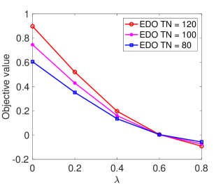
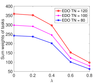
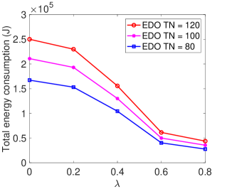
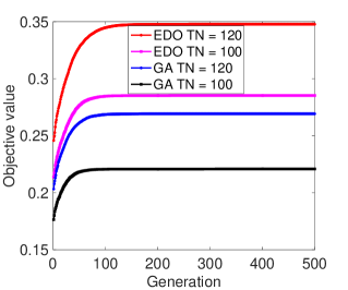
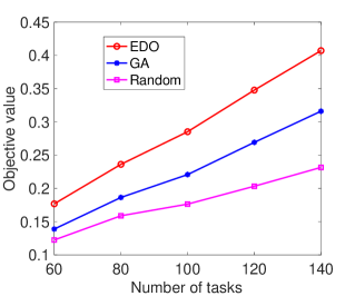
We adopt two experiments to verify the performance of the proposed EDO algorithm. In the first experiment, we first show the design objective value versus in Fig. 4, and then vary the values of to show the balance between two conflicting sub-objectives in Fig. 5, and Fig. 6. In the second experiment, we set to respectively evaluate the convergence and superiority of EDO in Fig. 7 and Fig. 8. We adopt the baselines of GA and Random to evaluate the performance of EDO. In GA, we use the solution in Section III-B to calculate the fitness value for each chromosome and power allocation is subject to the interval of . In Random, task scheduling and power allocation are randomly selected.
As depicted in Fig. 4, we show how the objective value obtained by EDO varies with for different task number (TN). From the objective value in Fig. 4, we further plot its two terms of the sum weights of tasks and the total energy consumption in Fig. 5 and Fig. 6, respectively. We can see that the objective value, the sum weights of tasks, and the total energy consumption decrease as grows. This result coincides well with our design objective function in P0. This is because that a larger value of favors the objective of minimizing the total energy consumption, while a smaller one favors the objective of maximizing the sum weights of tasks. This reveals a balance between the objectives of maximizing the sum weights of tasks and minimizing the total energy consumption. Furthermore, this phenomenon indicates that we can adjust the value of in practical applications to produce the desired metrics involving the sum weights of tasks and the total energy consumption.
In Fig. 7, we further show the comparisons between EDO and GA in terms of the objective value versus generations. From Fig. 7, we observe that the objective values obtained by both EDO and GA first increase with the number of tasks and then remain constant after 150 generations. This demonstrates that the proposed EDO achieves fast convergence in limited generations and provides a better convergence performance over GA.
In Fig. 8, we compare EDO with GA and Random in terms of the objective value versus the number of tasks. It is observed that the proposed EDO substantially outperforms the two comparison schemes in terms of the objective value as the number of tasks increase. This is because our proposed EDO jointly optimizes power allocation and task scheduling over a smaller feasible set of power to maximize the designed objective of P0. From Fig. 8, we can see that the objective value monotonically increases with the number of tasks increase. This is because that a smaller tends to maximize the sum weights of tasks instead of minimizing the total energy consumption.
V Conclusion
We study energy-efficient data offloading in EOSNs by jointly optimizing power allocation and task scheduling to minimize the total energy consumption and maximize the sum weights of tasks. We systematically explore the unique structures of joint optimization problem. We consider two special cases for the joint optimization problem and derive their near-optimal solutions. Then, we combine the two special solutions with genetic framework to propose an efficient two-layer EDO algorithm. Simulation results demonstrate the feasibility and effectiveness of the proposed algorithm.
References
- [1] J. Du, C. Jiang, Q. Guo, M. Guizani, and Y. Ren, “Cooperative earth observation through complex space information networks,” IEEE Wireless Commun., vol. 23, no. 2, pp. 136–144, Apr. 2016.
- [2] L. He, B. Liang, J. Li, and M. Sheng, “Joint observation and transmission scheduling in agile satellite networks,” IEEE Trans. Mobile Comput., vol. 21, no. 12, pp. 4381–4396, Dec. 2022.
- [3] D. Zhou, M. Sheng, J. Li, and Z. Han, “Aerospace integrated networks innovation for empowering 6G: A survey and future challenges,” IEEE Commun. Surveys Tuts., vol. 25, no. 2, pp. 975–1019, Feb. 2023.
- [4] J. Li, Z. Haas, and M. Sheng, “Capacity evaluation of multi-channel multi-hop ad hoc networks,” in IEEE ICPWC, New Delhi, India, Dec. 2002, pp. 211–214.
- [5] B. Deng, C. Jiang, L. Kuang, S. Guo, J. Lu, and S. Zhao, “Two-phase task scheduling in data relay satellite systems,” IEEE Trans. Veh. Technol., vol. 67, no. 2, pp. 1782–1793, Feb. 2018.
- [6] J. Li, G. Wu, T. Liao, M. Fan, X. Mao, and W. Pedrycz, “Task scheduling under a novel framework for data relay satellite network via deep reinforcement learning,” IEEE Trans. Veh. Technol., vol. 72, no. 5, pp. 6654–6668, May 2023.
- [7] N. Zufferey and M. Vasquez, “A generalized consistent neighborhood search for satellite range scheduling problems,” RAIRO-Oper. Res., vol. 49, no. 1, pp. 99–121, Jan. 2015.
- [8] Z. Liu, Z. Feng, and Z. Ren, “Route-reduction-based dynamic programming for large-scale satellite range scheduling problem,” Eng. Optim., vol. 51, no. 11, pp. 1944–1964, Jan. 2019.
- [9] Y. Chen, D. Zhang, M. Zhou, and H. Zou, “Multi-satellite observation scheduling algorithm based on hybrid genetic particle swarm optimization,” in AITIA, Berlin, Heidelberg, Jan. 2012, pp. 441–448.
- [10] Z. Zhang, F. Hu, and Z. Na, “Ant colony algorithm for satellite control resource scheduling problem,” Appl. Intell., vol. 48, no. 1, pp. 3295–3305, Feb. 2018.
- [11] J. Zhang and L. Xing, “An improved genetic algorithm for the integrated satellite imaging and data transmission scheduling problem,” Comput. Oper. Res., vol. 139, no. 1, pp. 1–11, Mar. 2022.
- [12] J. Qu, L. Xing, Y. Feng, M. Li, L. Jimin, Y. He, Y. Song, J. Wu, and G. Zhang, “Deep reinforcement learning method for satellite range scheduling problem,” Swarm Evol. Comput., vol. 77, no. 1, pp. 1–10, Jan. 2023.
- [13] J. Liang, J.-P. Liu, Q. Sun, Y.-H. Zhu, Y.-C. Zhang, J.-G. Song, and B.-Y. He, “A fast approach to satellite range rescheduling using deep reinforcement learning,” IEEE Trans. Aerosp. Electron. Syst., vol. 59, no. 6, pp. 9390–9403, Dec. 2023.
- [14] D. Zhou, M. Sheng, Y. Zhu, J. Li, and Z. Han, “Mission QoS and satellite service lifetime tradeoff in remote sensing satellite networks,” IEEE Wireless Commun. Lett., vol. 9, no. 7, pp. 990–994, Jul. 2020.
- [15] K. An, T. Liang, X. Yan, L. Y., and X. Qiao, “Power allocation in land mobile satellite systems: An energy-efficient perspective,” IEEE Commun. Lett., vol. 22, no. 7, p. 1374–1377, Jul. 2018.
- [16] Y. Ruan, Y. Li, C. X. Wang, R. Zhang, and H. Zhang, “Energy efficient power allocation for delay constrained cognitive satellite terrestrial networks under interference constraints,” IEEE Trans. Wireless Commun., vol. 18, no. 10, pp. 4957–4969, Oct. 2019.
- [17] S. Zhang, G. Cui, and W. Wang, “Joint data downloading and resource management for small satellite cluster networks,” IEEE Trans. Veh. Technol., vol. 71, no. 1, pp. 887–901, Jan. 2022.
- [18] X. Gao, J. Wang, X. Huang, Q. Leng, Z. Shao, and Y. Yang, “Energy-constrained online scheduling for satellite-terrestrial integrated networks,” IEEE Trans. Mobile Comput., vol. 22, no. 4, pp. 2163–2176, Apr. 2023.
- [19] A. Golkar and I. Lluch i Cruz, “The federated satellite systems paradigm: Concept and business case evaluation,” Acta Astron., vol. 111, pp. 230–248, Jun. 2015.
- [20] G. T. 38.811, “Study on new radio (NR) to support non-terrestrial networks,” Tech. Rep., Sept. 2020, V15.4.0.