On Supercapacitors Time–Domain Spectroscopy.
$C/R$ Characteristic Slope.

Abstract

$Id: timedomain.tex,v 1.399 2024/02/11 10:19:40 mal Exp $

A novel time-domain technique for supercapacitor characterization is developed, modeled numerically, and experimentally tested on a number of commercial supercapacitors. The method involves momentarily shorting a supercapacitor for a brief duration, denoted as $\tau$, and measuring first $\int Idt$ and second $\int I^{2}dt$ moments of current along with the potential before and after shorting. The effective $C(\tau)$ and $R(\tau)$ are then obtained from charge preservation and energy dissipation invariants. A linear behavior in $[R(\tau),C(\tau)]$ parametric plot is observed by several orders of $\tau$. This gives a $C/R$ characteristic slope: how much $\Delta C$ we can ‘‘gain’’ if we are ready to ‘‘lose’’ $\Delta R$ in internal resistance. The $C/R$ characteristic slope characterizes possible energy and power properties of the device in terms of materials and technology used, this is a measure of supercapacitor perfection. The technique has been proven with experimental measurements and then validated through computer modeling, analytic analysis, and impedance spectroscopy on a number of circuit types: transmission line, binary tree, etc., a new n-tree element (nTE) is introduced. The approach offers an alternative to low-frequency impedance spectroscopy and methods outlined in the IEC 62391 standard. It provides valuable insights into the performance and characteristics of supercapacitors.

1 Introduction

Distributed porous structure of supercapacitor electrodes lead to an equivalent circuit in the form of a distributed hierarchical $RC$ network that can be observed in electrical measurements[1, 2, 3, 4, 5, 6]. Supercapacitor measurement techniques can be classified as frequency domain (impedance spectroscopy) and time–domain (cyclic voltammetry, constant current charge/discharge regime[7, 8], etc.), see [9, 10, 11]. Multiple extensions to discharge techniques[12, 13, 14, 15, 16, 17, 18] have been recently proposed. In our previous work[19] we developed a pulse-discharge type of measurement technique that allows to determine, based on charge preservation invariant, the capacitance $C(\tau)$ available at discharge time $\tau$. In this work this approach has been extended and, based on energy dissipation invariant, the resistance $R(\tau)$ available at discharge time $\tau$ has been obtained. This $[R(\tau),C(\tau)]$ pair allows us to build a time–domain analogue of impedance spectroscopy $[\mathrm{Re}Z(\omega),\mathrm{Im}Z(\omega)]$.

Impedance spectroscopy is a powerful method to investigate properties of materials and electrodes reactions[20]. It is a frequency domain technique where the system is probed with low amplitude AC harmonic signal, the potential and current are measured with both amplitude and phase, then complex impedance $Z=U/I$ is obtained; frequency range varies by many orders, typically $10^{-3}\div 10^{6}~{}\mathrm{Hz}$, what allows to obtain information on porous structures. Interpretation is the most important step in impedance spectroscopy application. An analysis consists in assuming an equivalent circuit, then element values are optimized to fit theoretical and experimental curves, ZView is a common tool. Impedance spectroscopy application to supercapacitors characterization has it’s own specific. The supercapacitors equivalent circuit is simpler than the ones of a general electrochemical system and consists of a number of parallel and serial $RC$ branches corresponding to porous structure of electrode materials. An equivalent circuit of a porous system is a distributed $RC$ network; the elements like constant phase element (CPE) can be modeled with an infinite superposition of $RC$ branches[21].

The most common tool for presenting impedance spectroscopy theoretical and experimental results is Nyquist plot, which is a parametric plot of real and imaginary part of impedance $Z$ with frequency $\omega$ as a parameter: $[\mathrm{Re}Z(\omega),\mathrm{Im}Z(\omega)]$. For simple supercapacitor models the $Z(\omega)$ is a vertical half-line for serially connected $C$ and $R$, Fig. 1a and a half-circle of Cole-Cole style for parallel connection of $C$ and $R$ (self-discharge), Fig. 1b. The systems with half-line and half-circle are related to each other with the conformal mapping $Y=1/Z$ ($Y$ is complex admittance, an inverse to impedance $Z=1/Y$) that transforms[22, 23] a half-line into a half-circle, i.e. an electrochemical system with a vertical half-line (half-circle) in $[\mathrm{Re}Z(\omega),\mathrm{Im}Z(\omega)]$ would give a half-circle (vertical half-line) in $[\mathrm{Re}Y(\omega),\mathrm{Im}Y(\omega)]$. This is a general result. If the real/imaginary part of $Z$ (or $Y$) is a constant and the imaginary/real part depends arbitrary on a parameter $\xi$ (e.g. $\omega$, bias $U$, etc.) then a half-line in $[\mathrm{Re}Z(\xi),\mathrm{Im}Z(\xi)]$ is transformed to a half-circle in $[\mathrm{Re}Y(\xi),\mathrm{Im}Y(\xi)]$ and vice versa. For example in [24] we considered Fig. 1c system to plot an impedance $\left[\mathrm{Re}Z(U),\mathrm{Im}Z(U)\right]$ parametrically where the impedance was measured at fixed frequency with voltage bias $U$ (varied parameter) being applied to the system. The bias changed the value of $R(U)$, the value of $C(U)$ stayed constant. This corresponds to Fig. 1c $[\mathrm{Re}Y(U),\mathrm{Im}Y(U)]$ plot. When converted to $[\mathrm{Re}Z(U),\mathrm{Im}Z(U)]$ this gives vertically oriented half-circle.

In addition to impedance/admittance type of transform $Y=1/Z$ it may be beneficial to consider other conformal mappings such as $Y=1/(Z-R_{1})$ for example to a system with parallel connection of $R$ and $C$ with $R_{1}$ serially connected to them .

(a)
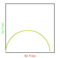
(b)
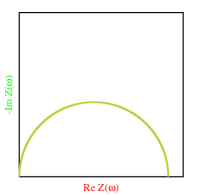
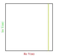
(c)

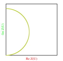
Figure 1: Several examples of impedance $Z$, admittance $Y=1/Z$, and their conformal mapping.

Whereas classic impedance theory deals with $[\mathrm{Re}Z(\omega),\mathrm{Im}Z(\omega)]$ basis (with conformal mapping possibly applied), this form is not very convenient in supercapacitor applications. First $\mathrm{Im}Z(\omega\to 0)$ diverges at small $\omega$, second this basis does not present directly how much energy/power the supercapacitor can possibly generate during $\tau$. In applications the most practical basis is capacitance vs internal resistance, a parametric plot with characteristic time $\tau$ as a parameter; this basis simultaneously characterizes energy and power properties of a SC. For traditionally measured complex $Z(\omega)$ the $C(\tau)$ and $R(\tau)$ can be introduced as (9) and (10) respectively with $\tau=1/\omega$ (8), this corresponds to $Z=R+\frac{1}{jwC}$. A parametric plot $[R(\tau),C(\tau)]$ (dashed olive line) is presented in Fig. 4b for a model system and in Fig. 8 for a real supercapacitor. This $[R(\tau),C(\tau)]$ is a non-conformal mapping of $[\mathrm{Re}Z(\omega),\mathrm{Im}Z(\omega)]$ with (9), (10). The plot is very convenient. The $R(\tau)$ and $C(\tau)$ increase together with $\tau$ as the electric current penetrates into deeper and deeper pores of supercapacitor material. A number of studies[25, 26, 27, 28] show strong dependence of supercapacitor properties not only on pores size, but also on their structure. These dependencies show contributions of different pore sizes, thus allow to predict the behavior at pulsed load[29] of different time length. The low/high $\tau$ asymptotes give minimal/maximal internal resistance and capacitance.

All these results are obtained in frequency domain, solely from $Z(\omega)$ impedance data. Impedance spectroscopy is a low current linear technique, non–linear effects are problematic to study[30]. At high AC amplitude the $Z(\omega)$ is measured in a non-linear regime what makes it difficult to interpret the results. The goal of this paper is to obtain the $[R(\tau),C(\tau)]$ from the measurements performed directly in time domain. Since the developed technique is based on the measurement of charge preservation and energy dissipation invariants – obtained $[R(\tau),C(\tau)]$ remains valid even when working in a highly non-linear regime. This allows us to take a completely new look into supercapacitor characterization.

2 Time Domain Spectroscopy: Theory and Modeling

In our previous work[19] a new technique for supercapacitors characterization, the inverse relaxation, has been developed. The technique consists in shorting a supercapacitor for a short duration $\tau$, then switching it to the open circuit regime and measuring an initial rebound and long-time relaxation. The current is measured during shorting stage. The main result of the previous work was to obtain the $C(\tau)$ that characterizes the distributiveness of $RC$ network. In this work the technique has been extended to obtain the $R(\tau)$.

For a distributed $RC$ network the $I(t),U(t)$ are measured in time–domain as presented in Fig. 2e. The main advantage of this time-domain measurement technique over impedance spectroscopy is that the measurements are performed in high-current regime that is similar to a typical regime of supercapacitors operation. Moreover, when impedance measurements are performed in a non–linear regime it is difficult[30] to interpret measured $Z(\omega)$ into capacitance and internal resistance. Since time domain interpretation is based on direct measurements of charge preservation and energy dissipation invariants — it remains valid even in a highly non-linear regime. The main disadvantage is that in impedance spectroscopy the $\omega$ can capture a wide range (at lest seven orders) of frequencies, but in time-domain measurement it is difficult to capture more than three orders of $\tau$.

bigskip

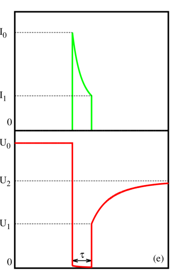
Figure 2: Supercapacitor equivalent circuit models: transmission line (a), superposition of $RC$ (b) and multi–branch; binary tree (c) is an example of a multi–branch model. Measurement circuit (d) and $U$, $I$ in time-domain (e).

Consider Fig. 2d circuit. Initially the switch ‘‘Short’’ is set to off, the switch ‘‘Charge’’ is set to on, the supercapacitor is charging; after a long enough time the switch ‘‘Charge’’ is set to off, the supercapacitor is considered charged. Then at $t=0$ the switch ‘‘Short’’ is set to on (shorting stage) and the $I(t)$ current is measured in the external circuit. At $t=\tau$ the switch ‘‘Short’’ is set to off, the current is interrupted. The $R_{s}$ is a small resistance used to measure the current, typically this is an internal resistance of wires and switches, it can be determined[19] using either four-terminal sensing technique or calibrated to total charge. Measuring $U_{s}$ we obtain the current $U^{*}/R_{s}=I$. If there is only a single $RC$ then on shorting stage ($R_{s}\ll R$) we have:

$$\frac{U^{*}}{R_{s}}=\frac{U}{R}=I =C\frac{dU}{dt}$$ (1)

For a single $RC$ circuit the values of $C$ and $R$ are exact values not depending on shorting time $\tau$. For a multi-branch $RC$ circuits in Fig. 2 the values can be interpreted as some $\tau$-dependent effective values $R(\tau)$ and $C(\tau)$ characterizing the supercapacitor. Integrating (1), we obtain:

$$Q =\int\limits_{0}^{\tau}I(t)dt=C\cdot(U_{0}-U_{1})$$ (2)

The total charge passed is calculated by integrating the current, the limits of integration can be extended to be the entire timeline since $I(t)=0$ for $t<0$ and $t>\tau$. Initial and final potentials $U_{0}$ and $U_{1}$ can be measured as the potentials before shorting and right after switching to open circuit regime. Obtain

$$C(\tau) =\frac{Q}{U_{0}-U_{1}}=\frac{\int I(t)dt}{U_{0}-U_{1}}$$ (3)

$$R_{1} =\frac{U_{0}}{I_{0}}=\frac{U_{1}}{I_{1}}$$ (4)

The $C(\tau)$ can be interpreted as an effective value characterizing the supercapacitor at shorting time $\tau$. The potential jump after shorting or after switching to the open circuit regime gives the lowest possible internal resistance $R_{1}$ (when the $R_{s}$ is not small as $R_{s}\ll R_{1}$ then (4) gives $R_{s}+R_{1}$). The $U_{0}$ and $U_{1}$ are supercapacitor’s potentials measured immediately before and immediately after shorting; the $I_{0}$ and $I_{1}$ are supercapacitor’s external circuit current measured immediately after and immediately before shorting. The $\tau$-dependent effective capacitance (3) and $\tau$-independent minimal internal resistance (4) are the result of [19].

The effective $R(\tau)$ characterizes how deep the current pulse of $\tau$ duration penetrates into the pores of supercapacitor material. Consider a single $RC$ circuit

(5)

if the potential on $C$ decreases from $U_{0}$ to $U_{1}$ with a single exponent evolution then $U_{1}=U_{0}\exp\left(\frac{-\tau}{R(\tau)C(\tau)}\right)$ and the effective resistance is:

$$\widetilde{R}(\tau) =\frac{\tau}{C(\tau)\ln\frac{U_{0}}{U_{1}}}$$ (6)

Whereas the capacitance estimation (3) is exact as it is based on charge preservation, the (6) is just an estimation based on an assumption of single exponent evolution of the potential; this does not hold true for multi-branch supercapacitors. We need $R(\tau)$ estimation that is based on an invariant. For a regular capacitor and (5) circuit the invariant is energy dissipation law $RI^{2}=\frac{1}{2}CdU^{2}/dt$, it follows from the dynamic equation (1) by multiplying it by $U$. Integrating, we obtain

$$R(\tau) =\frac{\left[U^{2}_{0}-U^{2}_{1}\right]C(\tau)}{2\int I^{2}(t)dt}=\frac{\left[U_{0}+U_{1}\right]\int I(t)dt}{2\int I^{2}(t)dt}$$ (7)

For a simple (5) circuit with regular capacitor it gives the exact value of $R$. With multi-branch capacitor that undergo multi-exponent dynamics the invariant no longer holds exactly. However it can be used to obtain $R(\tau)$ — an estimation of the effective internal resistance at $\tau$; it is determined from a condition of $\int I(t)dt$ and $\int I^{2}(t)dt$ relation. From (7) we obtain $R(\tau)$ asymptotes: $R(\tau\to 0)=R_{1}$ and $R(\tau\to\infty)=const$.

Whereas the $R_{1}$ from (4) characterizes the minimal possible internal resistance, the (7) characterizes the resistance of the whole system at $\tau$, it is an analogue of impedance real part at $\omega=1/\tau$. The idea is then to treat the $[R(\tau),\tau/C(\tau)]$ parametric plot as ‘‘real’’ and ‘‘imaginary’’ parts of system impedance.

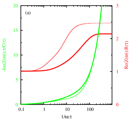
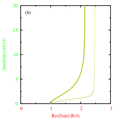
Figure 3: Modeling Fig. 2a circuit with $R_{1}=1\Omega$, $C_{1}=2F$, $R_{2}=1\Omega$, $C_{2}=5F$, $R_{3}=2\Omega$, $C_{3}=10F$ in time (solid lines) and frequency (dashed lines, $\tau=1/\omega$) domains. (a): real and imaginary part as a function on $\tau$; (b): parametric Nyquist plot $[\mathrm{Re}(Z),\mathrm{Im}(Z)]$. For time-domain the $R(\tau)$ and $\tau/C(\tau)$ are used instead of $\mathrm{Re}(Z)$ and $\mathrm{Im}(Z)$. Note, that a divergence of $\mathrm{Im}(Z(\tau\to\infty))$ makes this representation less convenient than $R(\tau)$, $C(\tau)$ in Fig. 4.

In Fig. 3 we present the result for a three-$RC$ system in Fig. 2a modeled (see A below) in time (solid lines) and frequency (dashed lines, $\tau=1/\omega$) domains. The imaginary part (green line) has the same $\tau\to 0$ and $\tau\to\infty$ asymptotes in both domains. A small difference is observed for intermediate $\tau$. The real part (red line) has the same $\tau\to 0$ asymptote in both domains, but $\tau\to\infty$ asymptote is different. The reason is that (7) averaging gives different (from impedance theory) weights to deep branches.

The basis $[\mathrm{Re}(Z),\mathrm{Im}(Z)]$ is not very convenient for characterizing supercapacitors. First, the $\mathrm{Im}(Z)$ is not bounded, it diverges at $\tau\to\infty$ (corresponds to $\omega\to 0$) if there is no self-discharge. Second, accumulated energy is proportional to $C$, thus it is convenient to present the $C$ explicitly. For time–domain the $C(\tau)$ is given by (3), for frequency domain let us define it as (9). There are other ways to introduce $C_{impedance}(\tau)$, for example similar to Fig. 1 above we can introduce $Y=1/Z$ and consider the value $\mathrm{Im}Y/\omega$. However, this would be more appropriate for the systems with parallel $RC$; for supercapacitors the discharge is typically small and the (9) definition is reasonable. Thus the most convenient variables to characterize a supercapacitor from measured impedance data $[\mathrm{Re}Z(\omega),\mathrm{Im}Z(\omega)]$ are

$$\tau =\frac{1}{\omega}$$ (8)

$$C_{impedance}(\tau) =\frac{-1}{\omega\mathrm{Im}Z(\omega)}=\frac{-\tau}{\mathrm{Im}Z(1/\tau)}$$ (9)

$$R_{impedance}(\tau) =\mathrm{Re}Z(\omega)=\mathrm{Re}Z(1/\tau)$$ (10)

A similar approach to consider $[R,C]$ basis instead of $[\mathrm{Re}Z(\omega),\mathrm{Im}Z(\omega)]$ was introduced in [17] in application to supercapacitors and in [32] in application to perovskite-graphene oxide composite films. Whereas for the films the $[R,C]$ are just some characteristics of the material, for supercapacitors the $[R,C]$ are the most important characteristics and presenting them in the same plot gives a much better understanding of the device characteristics.

In time-domain the values of $C(\tau)$ and $R(\tau)$ are obtained directly, no conversion necessary. The expressions (9) and (10) of frequency domain correspond exactly to (3) and (7) of time-domain. In Fig. 4 we present the result for the same three-$RC$ system in Fig. 2a in $[R(\tau),C(\tau)]$ basis; time domain is in solid line, frequency domain is in dashed line. As expected $\tau\to 0$ asymptotes match as $R(\tau\to 0)=R_{1}$ and $C(\tau\to 0)=C_{1}$; the $C(\tau\to\infty)$ asymptotes matches exactly the total capacitance $C(\tau\to\infty)=C_{1}+C_{2}+C_{3}+\dots$, for $R(\tau\to\infty)$ the asymptotes are different in time and frequency domains. Most manufacturers provide equivalent ESR at fixed frequency $1000~{}\mathrm{Hz}$ in the datasheets, which is typically several times lower than the internal resistance at DC. In [19] a chart of supercapacitor’s internal $RC$ time as a function of capacitance was made for a number of supercapacitors based on manufacturers datasheets. In Fig. 4c the $R(\tau)C(\tau)$ is presented as a function of shorting time $\tau$ for a single supercapacitor, the dependence of supercapacitor internal time on shorting time $\tau$. If we divide accumulated energy $CU^{2}/2$ by current power $U^{2}/R$ the ratio (within a factor of 2) will be the supercapacitor internal time $R(\tau)C(\tau)$. It characterizes the distribution of the internal porous structure of the system.

The parametric plot $[R(\tau),C(\tau)]$ (Fig. 4b, olive) is the most informative. It shows how the supercapacitor behaves at different $\tau$. The $R(\tau)$ and $C(\tau)$ increase together with $\tau$ as the electric current penetrates into deeper and deeper pores of supercapacitor material. This $[R(\tau),C(\tau)]$ parametric plot shows what energy and power can be possibly obtained from a supercapacitor at a given time–scale $\tau$. For device properties analysis it is more convenient than regular Nyquist plot $[\mathrm{Re}Z,\mathrm{Im}Z]$ that requires equivalent circuit fitting.

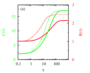
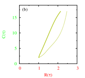
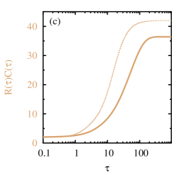
Figure 4: Modeling Fig. 2a circuit with $R_{1}=1\Omega$, $C_{1}=2F$, $R_{2}=1\Omega$, $C_{2}=5F$, $R_{3}=2\Omega$, $C_{3}=10F$ in time (solid lines) and frequency (dashed lines, $\tau=1/\omega$) domains. (a): effective $R$ and $C$ as a function on $\tau$; (b): parametric $[R(\tau),C(\tau)]$ plot that exhibits close to linear behavior even in this simple three-$RC$ model; (c): The effective internal $RC$ time as a function on $\tau$.

2.1 Time–Domain Modeling of Various Equivalent Circuits

Equivalent circuits used to describe supercapacitors electric properties typically contain several building blocks shown in Figs. 2a,b,c. It is well known [11, 20] that different equivalent circuits can provide identical impedance behavior; different SC models containing more than a dozen of $RC$ elements create a good fit to almost any experimental data.

A transmission line model (horizontal ladder network) is very popular in the supercapacitors community[33, 34, 35, 36]. It considers a number of $RC$ elements connected in chain, Fig. 2a. Alternatively one can model a supercapacitor with a number of $RC$ elements connected in parallel (superposition, vertical ladder network), Fig. 2b. Given sufficient number of $RC$ elements both circuits fit various experimental data well, for example Fig. 2b can be used to model a CPE element[21]. Good fitting with a complex circuit, however, does not guarantee that a supercapacitor has exactly this equivalent circuit on material level.

A generalization of these models is multi-branch circuits where an element at $k$-th level is connected to more than one element at $k+1$-th level, a tree-like equivalent circuit[37, 38, 39]. Binary tree, where $k$-th level node is connected to two $k+1$-th level nodes (exactly two descendant nodes) is a simple example of multi–branch, see Fig. 2c, it has exactly $2^{k}$ capacitors (and resistors) at $k$-th level, totally $2^{k+1}-1$ capacitors (and resistors) on all levels below or equal $k$. It is convenient to numerate elements with two indexes: level $k$ and element number within level $m=1\dots 2^{k}$. If all the capacitors (and resistors) for a given level $k$ are the same, i.e. $C_{km}$ (and $R_{km}$) do not depend on $m$ then, considering system symmetry, one can immediately obtain an equivalence to transmission line model[38] with

$$C_{k} =C_{k*}\cdot 2^{k}$$ (11a)

$$R_{k} =R_{k*}/2^{k}$$ (11b)

(for such a high symmetry system the potential is the same for all capacitors in the $k$-th level). A binary tree with $C_{km}=0$ and $R_{km}=0$ for all $k$ except the one equals to the tree depth (max level) is equivalent to superposition model in Fig. 2b. For a binary tree with arbitrary $RC$, as well as for a tree with varying number of descendant nodes, this equivalence to Fig. 2a,b simple models no longer holds. Note, that one can represent an arbitrary (e.g. having varying number of child nodes) $RC$ network of tree structure with a binary tree by inserting dummy elements with properly chosen $R$ and $C$, similarly to an equivalence of transmission line and superposition models to a binary tree of special form.

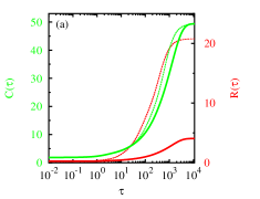
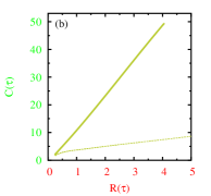
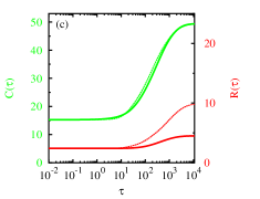
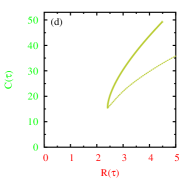
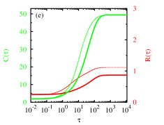
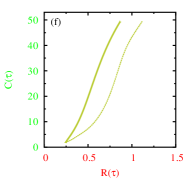
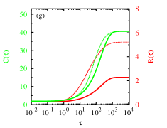
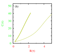
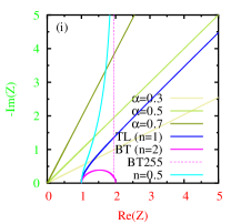
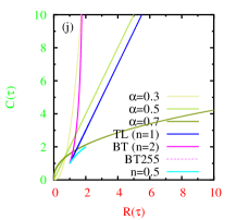
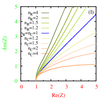
Figure 5: Modeling $RC$-network circuits. In time (solid line) and frequency (dashed line) domains: (a), (b) – Fig. 2a transmission line model with $31$ random $RC$ elements; (c), (d) – Fig. 2b superposition model with $31$ random $RC$ elements; (e), (f) – Fig. 2c binary tree model of depth $4$, $31$ random $RC$ elements; (g), (h) – Fig. 2c binary tree model of depth $7$, $255$ random $RC$ elements. Modeling in frequency domain to compare with CPE: (i), (j) – CPE element with $\alpha=\{0.3,0.5,0.7\}$ (17), infinite transmission line TL (13), binary tree — infinite BT (21), of $255$ identical $RC$ elements BT255, and $n=0.5$ weakly linked n-tree (23). (k) nTE – n-tree element (23) exhibits deformed semi-circles of Cole-Cole style for $n>1$. (l) CPE modeling with self-similar $RC$ network (26) of $100$ $RC$ elements for different $n_{C}$, $n_{R}=1$ when $\alpha<0.5$, and $n_{R}$, $n_{C}=1$ when $\alpha>0.5$, see C.

To create $RC$ networks in Fig. 2 we need to define a distribution for $R$ and $C$. In this paper the log-normal distribution is used for the reason to minimize the number of parameters and to avoid the problem with negative values when normal distribution is used. For a number of $RC$ networks we plot $R(\tau)$, $C(\tau)$, and $[R(\tau),C(\tau)]$ parametric plot in time and frequency domains. The $[\mathrm{Re}Z(\omega),\mathrm{Im}Z(\omega)]$ plots are much less informative since $\mathrm{Im}Z(\omega)$ diverges at $\tau\to\infty$, see Fig. 3. The $C(\tau)$ has known $\tau\to 0$ and $\tau\to\infty$ asymptotes. If there is no discharge – they are identical both in time and frequency domains as well as the $R(\tau\to 0)$. The $C(\tau\to\infty)$ is the sum of all $C$ of the network.

In Fig. 5a,b the transmission line model, Fig. 2a, of $31$ random $RC$ elements is presented; the value of $31$ is chosen to simplify the comparison below with binary tree model of depth $k=4$ that has $2^{k+1}-1$ capacitors (and resistors). The network is built as $C=\exp(\mathcal{N}(0,1))$, $R=\exp(\mathcal{N}(0,1))$, where $\mathcal{N}(0,1)$ is Gaussian random variable with zero mean and unit variance, standard normal distribution. We observe almost perfect linear dependence in $[R(\tau),C(\tau)]$ parametric plot. The $C/R$ slope is different in time and frequency domains. Linear dependence is observed by six orders of $\tau$, but only four orders of $\tau$ range are informative as a plateau in $R(\tau)$ and $C(\tau)$ is reached outside of the range.

This $[R(\tau),C(\tau)]$ parametric plot linear behavior is a general property of transmission line model. An analytic solution in frequency domain can be obtained in some cases. Consider Fig. 2a model of infinite length of identical $RC$: $R_{k}=R$ and $C_{k}=C$. Since adding one more $RC$ element to an infinite chain does not change the $Z(\omega)$, we obtain:

$$Z =R+\frac{Z\frac{1}{j\omega C}}{Z+\frac{1}{j\omega C}}$$ (12)

$$Z(\omega) =\frac{R}{2}\pm\sqrt{\frac{R^{2}}{4}+\frac{R}{j\omega C}}$$ (13)

$$\frac{\Delta C}{\Delta R} =\frac{\frac{dC_{impedance}}{d\omega}}{\frac{dR_{impedance}}{d\omega}}=\frac{\displaystyle\frac{d}{d\omega}\frac{-1}{\omega\mathrm{Im}Z(\omega)}}{\displaystyle\frac{d}{d\omega}\mathrm{Re}Z(\omega)}$$ (14)

$$\frac{\Delta C}{\Delta R} =\frac{2C}{R}$$ (15)

Impedance $Z(\omega)$ of Fig. 2a infinite chain of identical $RC$ is obtained as quadratic equation solution; the solution corresponds to ‘‘$+$’’ sign in (13) when the square root operation is defined as having positive real part. From (13), after simple algebra and symbolic calculations, see B below, it immediately follows that in variables $R_{impedance}(\tau)$ from (10) and $C_{impedance}(\tau)$ from (9) the parametric plot $[R_{impedance}(\tau),C_{impedance}(\tau)]$ for transmission line of infinite length is linear with $C/R$ slope equals exactly to $2C/R$ from (15):

$$C_{impedance}(\tau) =\frac{2C}{R}R_{impedance}(\tau)-C$$ (16)

A close to linear law also holds for a finite length transmission line with $RC$ elements having randomness, see Fig. 5b. When a finite length transmission line is considered in variables $[\mathrm{Re}Z(\omega),\mathrm{Im}Z(\omega)]$, as it is typically done for SC, the $\mathrm{Im}Z(\omega)$ diverges at $\omega\to 0$ as in Fig. 3b and the system is hard to identify. This non-conformal mapping from $[\mathrm{Re}Z(\omega),\mathrm{Im}Z(\omega)]$ to $[R(\tau),C(\tau)]$ allows us easily identify a transmission line: if there is a linear dependence in $[R(\tau),C(\tau)]$ parametric plot – there is a transmission line model corresponding to this $Z(\omega)$. For time-domain consideration we cannot obtain an analytic solution. Numerical experiments with very long transmission lines (from $100$ to $500$ identical $RC$ elements) show linear dependence in time domain, the $[R(\tau),C(\tau)]$ parametric plot is almost linear by five orders of $\tau$ range, Eqs. (3) and (7). The $C/R$ slope is higher than the one in frequency domain, in time domain it varies from $4.8C/R$ at low $\tau$ to $7.5C/R$ at high $\tau$, compare this with the exact value of $2C/R$ in frequency domain (15). This leads us to conclude that linear $[R(\tau),C(\tau)]$ parametric plot is an intrinsic property of a transmission line model.

Exactly linear $C/R$ slope is not unique to transmission line with $Z(\omega)$ from (13). Consider CPE element[40, 21] in frequency domain. It has

$$Z(\omega) =\frac{1}{(j\omega)^{\alpha}C_{\alpha}}$$ (17)

$$-1 \leq\alpha\leq 1$$ (18)

The case $\alpha=1$ corresponds to regular capacitance, $\alpha=-1$ corresponds to inductance. In $[\mathrm{Re}(Z),\mathrm{Im}(Z)]$ parametric plot we have a line with the slope determined by the value of $\alpha$, see Fig. 5i. Let us apply non-conformal mapping to obtain $R_{impedance}(\tau)$ from (10) and $C_{impedance}(\tau)$ from (9) for different values of $\alpha$. The result is presented in Fig. 5i,j. One can clearly see that $\alpha=0.5$ CPE case (diffusion limited process) has exactly linear dependence in $[R(\tau),C(\tau)]$ parametric plot. The slope is the same as for transmission line Eq. (13): compare blue $n=1$ line (infinite transmission line with $R=1\Omega$, $C=1F$) and olive line of $\alpha=0.5$ CPE element with $C_{\alpha}=1$ . Transmission line is a good model[40] for diffusion-limited CPE with $\alpha=0.5$; a shift is due to $R/2$ term in (13).

In Fig. 5c,d the superposition model, Fig. 2b, of $31$ random $RC$ elements is presented. The network is built as $C=\exp(\mathcal{N}(0,1))$, $R=100\exp(\mathcal{N}(0,1))$, a factor of $100$ is chosen to bring the effective $R$ of the network to approximately the same range as for other models, note that $R(\tau\to 0)=1\big{/}\sum\limits_{k}1/R_{k}$. This Fig. 2b model has the most noticeable deviation from linearity in $[R(\tau),C(\tau)]$ parametric plot since it has no deep branches. Linear dependence is observed by a singe order of $\tau$ range. At small $\tau$ the $C(R)$ plot convexity (deviation from linear law) for the model has an opposite sign than for the experimental data in Fig. 8. For a superposition model with identical elements an analytic solution can be obtained both in time and frequency domains. The system with $n$ identical $\widetilde{R}\widetilde{C}$ elements is equivalent to a single $RC$ of (5) form with $R=\widetilde{R}/n$ and $C=\widetilde{C}n$. This single $RC$ circuit has no distributed branches and its parametric plot $[R(\tau),C(\tau)]$ is a single point $[R,C]$ both in time and frequency domains.

In Fig. 5e,f a binary tree model, Fig. 2c, of depth four ($31$ random $RC$ elements) is presented. The network is built as $C=\exp(\mathcal{N}(0,1))$, $R=\exp(\mathcal{N}(0,1))$. The model has little deviation from linearity and, contrary to transmission line results in Fig. 5a,b, the $C/R$ slope is very similar in time and frequency domains; similar behavior has also been observed in experimental data in Fig. 8. At small $\tau$ the $C(R)$ plot convexity for the model has the same sign as in the experimental data.

In Fig. 5g,h the binary tree model, Fig. 2c, of depth seven ($255$ random $RC$ elements) is presented; this value is chosen to be able to consider depth-dependent factors while in the same time not to have too many $RC$ elements to avoid any possible numerical instabilities. The network is built as:

$$C_{km} =\exp(\mathcal{N}(0,1))/\beta_{C}^{k}$$ (19a)

$$R_{km} =\exp(\mathcal{N}(0,1))\beta_{R}^{k}$$ (19b)

Different for $C$ and $R$ depth-dependent factors $\beta_{C}$ and $\beta_{R}$ are introduced to construct a more realistic $RC$ distribution. They partially compensate growing number of elements with tree depth increase. If $\beta_{C}=\beta_{R}=2$ then these factors totally compensate (11) and this $RC$ network becomes similar to the transmission line model. In Fig. 5g,h we put $\beta_{C}=1.5$ and $\beta_{R}=1.8$, thus only partial compensation takes place. The $C/R$ is still almost linear in time-domain and there is a noticeable difference from $C/R$ value in frequency domain, a behavior we already observed in random transmission line model in Fig. 5a,b.

For an infinite binary tree with identical $RC$ elements an analytic solution in frequency domain can be obtained. Since adding one more $RC$ level to an infinite binary tree does not change the $Z(\omega)$, we obtain a recurrent relation that leads to quadratic equation solution:

$$Z =R+\frac{Z\frac{1}{2j\omega C}}{Z/2+\frac{1}{j\omega C}}$$ (20)

$$Z(\omega) =\frac{1}{2}\left[R-\frac{1}{j\omega C}\right]\pm\sqrt{\frac{1}{4}\left[R-\frac{1}{j\omega C}\right]^{2}+\frac{2R}{j\omega C}}$$ (21)

The calculation of $C/R$ slope Eq. (14), however, does not give a constant as it is for transmission line model in Eq. (15), the $C/R$ slope changes slightly with $\omega$. Overall the result is similar to a binary tree with log-normal distribution of $R$ and $C$. The exact result is shown in Fig. 5i,j in pink: for an infinite binary tree BT (solid), for a binary tree of depth $7$ ($255$ identical $RC$) BT255 (dashed); they differ only at very small $\omega$. A remarkable feature of the binary three model is that a Cole-Cole style semi-circle can be obtained without charge leak, see Fig. 5i and compare it with Fig. 1b; this binary tree corresponds to the transmission line with $RC$ values depending on $k$ as Eq. (11). The $[\mathrm{Re}Z(\omega),\mathrm{Im}Z(\omega)]$ plot is a deformed semi-circle with $\mathrm{Re}Z(\omega\to\infty)=R$, $\mathrm{Re}Z(\omega\to 0)=2R$, and $\mathrm{Im}Z(\omega\to\infty)=\mathrm{Im}Z(\omega\to 0)=0$ asymptotes. The $\mathrm{Im}Z(\omega\to 0)=0$ holds only for an infinite tree, for a finite size tree it starts showing a capacitance-like behavior at some low $\omega$, see BT255 dashed pink line in Fig. 5i.

One can generalize Eqs. (12) and (20) recurrence to a tree with an arbitrary number of descendants $n$:

$$Z =R+\frac{Z\frac{1}{nj\omega C}}{Z/n+\frac{1}{j\omega C}}$$ (22)

$$Z(\omega) =\frac{1}{2}\left[R+\frac{1-n}{j\omega C}\right]\pm\sqrt{\frac{1}{4}\left[R+\frac{1-n}{j\omega C}\right]^{2}+\frac{Rn}{j\omega C}}$$ (23)

We name this infinite $RC$-network of identical $RC$ elements as the n-tree element (nTE), this is a special case of a general tree-like system[37]. The $n=1$ corresponds to transmission line model (single descendant), $n=2$ corresponds to binary tree model (two descendants). The value of $n$ determines tree growth exponent. In quadratic equation solution the sign is ‘‘$+$’’ in (23) when the square root operation is defined as having positive real part. A weakly linked ($n<1$) n-tree with $n=0.5$ is presented in Fig. 5i,j in light blue; this model has bounded total $C$, thus $C(\tau\to\infty)$ does not diverge for an infinite $RC$ network. nTE asymptotes for $n<1$ are: $R_{impedance}(\tau\to\infty)=R/(1-n)$, $C_{impedance}(\tau\to\infty)=C/(1-n)$, $R_{impedance}(\tau\to 0)=R$, $C_{impedance}(\tau\to 0)=C$. The $[R_{impedance}(\tau),C_{impedance}(\tau)]$ parametric plot is close to linear but not exactly. Average $C/R$ slope for $n<1$ is approximately equal to $C/R$ what is about twice lower than the value in $n=1$ case, Eq. (15). At $n=1$ tree-like $RC$ network in question has a percolation phase transition observed in $C(\tau\to\infty)$ divergence; at $n\geq 1$ the total capacitance of nTE becomes infinite, i.e. the capacitance becomes limited by the device actual size. Percolation properties of supercapacitor electrodes are actively studied in recent works [41, 42, 43, 44].

For $n>1$ the n-tree model produces deformed semi-circle in $[\mathrm{Re}Z(\omega),\mathrm{Im}Z(\omega)]$ with asymptotes: $\frac{\Delta C}{\Delta R}\Big{|}_{\omega\to\infty\mkern-36.0mu}=(n+1)\frac{C}{R}$, $\mathrm{Re}Z(\omega\to\infty)=R$, $\mathrm{Re}Z(\omega\to 0)=\frac{n}{n-1}R$, and $\mathrm{Im}Z(\omega\to\infty)=\mathrm{Im}Z(\omega\to 0)=0$; the $\mathrm{Im}Z(\omega\to 0)=0$ holds only for an infinite $RC$ network. In Fig. 5k we present n-tree models with different values of $n>1$. Deformed semi-circles are clearly observed. Since carbon structures of supercapacitor electrodes are hierarchical tree-like structures this leads us to conclude that SC impedance semi-circles as in Fig. 1b on material level can be explained by a n-tree model with $n>1$. The n-tree model of identical $RC$ elements is equivalent to a transmission line model in Fig. 2a with $k$-dependent $C_{k}=n^{k}C$ and $R_{k}=R/n^{k}$. See B below for symbolic and numerical calculation of $Z(\omega)$ from (23), the command ‘‘python3 n-tree_element.py 1.25’’ calculates n-tree impedance for a given number of descendants $n=1.25$.

The modeling above leads us to conclude that linear $C/R$ behavior can be observed in various $RC$ networks with deep branches. The systems without deep branches, such as in Fig. 2b, have noticeable deviation from the linear law. The C/R slope in time- and frequency- domains is similar in some systems (such as binary tree) and significantly different in others (such as transmission line). Time domain technique uses (3) and (7) to directly measure the $C(\tau)$ and $R(\tau)$; frequency domain technique measures the impedance $Z(\omega)$ first, then uses Eqs. (9) and (10) to convert impedance data to effective $C$ and $R$; the limitations of Eqs. (9) and (10) makes the result much less accurate. However, for some systems, e.g. binary tree modeling in Fig. 5e,f and experimental data in Fig. 8, the $C/R$ slope is very similar in time and frequency domains. A minimal system to observe a close to linear $[R(\tau),C(\tau)]$ dependence is Fig. 2a transmission line model with three $RC$ elements, see Fig. 4b.

3 Supercapacitors Experimental Measurements in Time Domain

The modeling of previous section shows the value of developed technique. Consider its practical application. In experiments we tested the approach on four commercial supercapacitors, see Fig. 6 for the list, with the initial potential $U_{0}=2.5V$; these supercapacitors all have $5F$ nominal capacitance and are $2.7V$ rated. Shorting time duration $\tau$ was taken $10^{-2}$ to $10^{2}~{}\mathrm{s}$, the $[10^{-2}\div 10]~{}\mathrm{s}$ is an informative interval as the plateau is reached at $\tau>10~{}\mathrm{s}$.

To obtain $[R(\tau),C(\tau)]$ we need to know the integrals $\int Idt$ (3) and $\int I^{2}dt$ (7) of current, they correspond to total charge and dissipated energy respectively. The measurement is implemented with STM32F103C8T6 ARM microcontroller. Operational amplifier AD823 brings small potential on shorting stage to the range of maximal ADC precision. We calculate current moments by direct integration:

$$Q(\tau)=\int\limits_{0}^{\tau}Idt \approx\sum\limits_{k}\frac{U(t_{k})}{R_{s}}(t_{k}-t_{k-1})$$ (24)

$$\int\limits_{0}^{\tau}I^{2}dt \approx\sum\limits_{k}\frac{U^{2}(t_{k})}{R^{2}_{s}}(t_{k}-t_{k-1})$$ (25)

‘‘Right rectangle’’ integration rule is used to simplify microcontroller implementation, it is more than adequate for a typical sampling frequency $10^{5}/\mathrm{s}$. Previously considered[19] minimal internal resistance (4) requires only a jump in potential. Similar current–interruption technique is often used in fuel cell measurements [47], page 64, the immediate rise voltage $V=IR_{i}$ is an analogue of $U_{1}-U^{*}$; the [47] technique is equivalent to Eq. (4), where current interruption from $I_{1}$ to $0$ gives immediate rise (initial rebound) $R_{1}I_{1}=U_{1}-U^{*}$ of the potential what allows to determine the minimal resistance $R_{1}$ (and only the $R_{1}$). Eq. (7) has a major advantage over this current interruption technique. It uses second order moment of current (25) and the $R(\tau)$, which contains information about internal $RC$ distribution, is obtained. Another advantage is that (25) calculates an integral over the entire shorting interval, what makes it less measurement error prone compared to the measurement of immediate rise voltage that is a single point observation what can possibly give some discrepancy in practical measurements. With accurate measurement (confirmed by the modeling) we always have $R_{1}=R(\tau\to 0)$, the minimal possible $R(\tau)$.

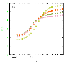
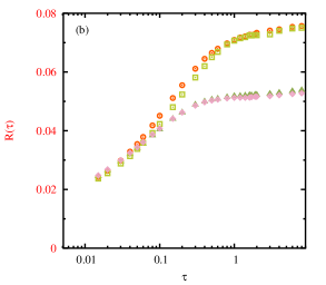
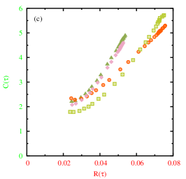
Figure 6: Experimental measurement of (а): $C(\tau)$ (3), (b): $R(\tau)$ (7), and (c): $[R(\tau),C(\tau)]$ parametric plot with a clear linear dependence observed (similar to Fig. 4b modeling). The results are presented for four commercial supercapacitors AVX-SCCS20B505PRBLE (circles), Eaton-HV1020-2R7505-R (triangles), IC-505DCN2R7Q (squares), and Nesscap-ESHSR-0005C0-002R7 (rhombuses). They have $C/R$ characteristic slope of $65F/\Omega$, $111F/\Omega$, $92F/\Omega$ and $107F/\Omega$ respectively.

Experimental results are similar to Figs. 4 and 5 modeling. Both $R(\tau)$ and $C(\tau)$ grow with $\tau$ increase. The most informative is a parametric plot $[R(\tau),C(\tau)]$ in Fig. 6c. With $\tau$ above some value the $[R(\tau),C(\tau)]$ is almost linear function, even more linear than three $RC$ transmission line model in Fig. 4b, a convexity at low $\tau$ make the plot similar to binary tree model in Fig. 5e,f. Initial $R$-offset is determined by the contacts. The slope $\Delta C/\Delta R$ is the most important characteristic determining possible power properties of the device in terms of materials and technology used. We call it $C/R$ characteristic slope (measured in $F/\Omega$): how much $\Delta C$ we can ‘‘gain’’ if we are ready to ‘‘lose’’ $\Delta R$ in internal resistance. From the data in Fig. 6c it immediately follows that the maximal characteristic slope is $111F/\Omega$ for Eaton-HV1020-2R7505-R (triangles) and the minimal characteristic slope is $65F/\Omega$ for AVX-SCCS20B505PRBLE (circles). This linear $C/R$ dependence, measured completely in time domain is the major result of this work. The $C/R$ characteristic slope can be viewed as a measure of supercapacitor perfection.

A SC, when probed at different time scales, has charge penetration to pores increasing with time scale. The equivalent capacitance growths. But the equivalent internal resistance also growths. The perfection is considered as a relative contribution of deep pores to capacitance and to internal resistance. The more deep pores contribute to capacitance and the less to resistance — the better supercapacitor is. Their relative contribution is determined by the slope in $[R(\tau),C(\tau)]$ parametric plot.

4 Supercapacitors Experimental Measurements in Frequency Domain

Obtained in previous section time–domain $C/R$ linear dependence is an important new result. From methodological point of view, to prove the technique, we consider the same $C/R$ dependence in frequency domain. As we emphasized above the Eqs. (9) and (10) are not accurate for real supercapacitors, however in this section we apply them to supercapacitors assuming no charge leak. Impedance data is measured in frequency range $10^{-2}\div 10^{3}~{}\mathrm{Hz}$ with $10mV$ AC amplitude. Nyquist plot for IC-505DCN2R7Q is presented in Fig. 7a. The impedance was measured with two values of bias applied: $0V$ and $1.5V$; it is typical for supercapacitors to have the parameters slightly changed under bias applied.

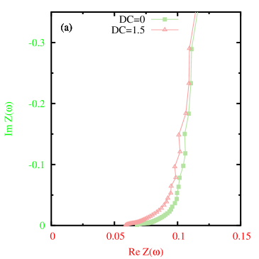
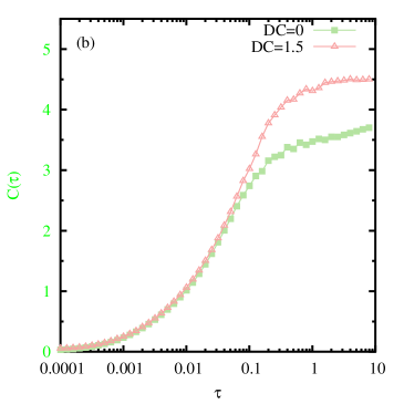
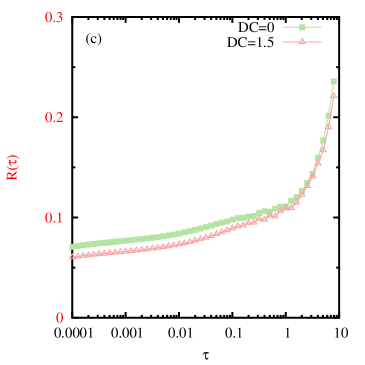
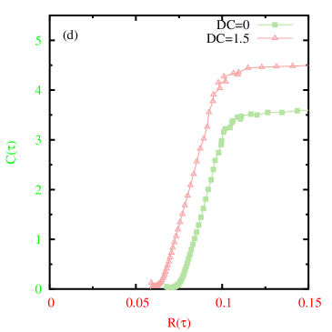
Figure 7: For IC-505DCN2R7Q supercapacitor. (a) Original Nyquist plot. (b) $C(\tau)$ dependence (9). (c) $R(\tau)$ dependence (10). (d) The $[R(\tau),C(\tau)]$ parametric plot. A linear dependence is clearly observed within two orders of $\tau$. Compare with Fig. 6c.

In Fig. 7b,c the $C(\tau)$ (9) and $R(\tau)$ (10) are presented. The $R(\tau)$ is valid only for $\tau\lesssim 1~{}\mathrm{s}$, then it diverges. The divergence is caused both by limited applicability of Eqs. (9), (10) and increased measurement errors at low frequencies. The $C(\tau)$ is valid for $\tau\gtrsim 10^{-2}~{}\mathrm{s}$, due to limited applicability of Eq. (9).

However, if we do $[R(\tau),C(\tau)]$ parametric plot, see Fig. 7d, we observe a linear dependence in the range $10^{-2}\leq\tau\leq 1$, similar to the one in Fig. 6c measured in time domain. The $C/R$ characteristic slope is about $110F/\Omega$; this is similar to $92F/\Omega$ value in time domain. A comparison is presented in Fig. 8. The $C/R$ characteristic slope is almost the same; the absolute values are shifted due to limitation of Eqs. (9) and (10) frequency domain estimation. Close to linear $[R(\omega),C(\omega)]$ parametric plot was observed (in frequency domain) experimentally by other researchers, see Fig. 2c of [17] where it is about $0.013F/\Omega$ for NEC supercapacitor part #FGR0H105ZF, $1F$, $5.5V$ rated (two SC are connected in serial, the $C/R$ slope is four times lower than for a single SC). Here we observe a linear $[R,C]$ parametric plot both in time- and frequency- domains for a number of different SC.

This leads us to conclude that linear dependence in parametric plot $[R(\tau),C(\tau)]$ within several orders in $\tau$ is a very general property of distributed $RC$ systems, it can be observed both in time and frequency domains. It measures supercapacitor perfection.

Figure 8: A comparison of $C/R$ characteristic slope for IC-505DCN2R7Q measured in time domain Fig. 6c (squares) and frequency domain Fig. 7d (triangles). A linear dependence is clearly observed in both cases. See Fig. 4b and Fig. 5b,f for modeled systems.

5 Discussion

In this work a novel time-domain measurement technique for supercapacitors characterization is developed, modeled numerically, and experimental testing on a number of commercial supercapacitors was conducted to validate it. The technique consists in shorting a supercapacitor on $\tau$ duration and measuring first $\int Idt$ and second $\int I^{2}dt$ moments of current along with the potential before and after shorting. The effective $C(\tau)$ and $R(\tau)$ are then obtained from charge preservation and energy dissipation invariants. The approach can be considered as an alternative/extension to commonly used [7] DC-ESR technique, see Maxwell datasheet; we have an effective resistance $R(\tau)$ calculated at different values of $\tau$.

Among new results obtained with the developed time-domain technique is an observation of linear behavior in $[R(\tau),C(\tau)]$ parametric plot that characterizes the device in terms of materials and technology used. The $C/R$ characteristic slope is a constant within several orders of $\tau$, this has been confirmed in Section 2.1 modeling on a number of circuit types: transmission line, binary tree, etc. The result is also confirmed with impedance technique; whereas in impedance spectroscopy typically only conformal mapping (such as impedance/admittance $Y=1/Z$, see Fig. 1) are considered, we have shown that non-conformal mapping from $[\mathrm{Re}Z(\omega),\mathrm{Im}Z(\omega)]$ to $[R(\tau),C(\tau)]$ allows to obtain the $C/R$ characteristic slope (however time-domain measurement is more accurate as no conversion required). A linear dependence in $[R(\omega),C(\omega)]$ parametric plot in frequency domain was experimentally observed in [17], this confirms our results. The $[R(\tau),C(\tau)]$ when directly measured in time domain gives the most accurate results (compared to frequency domain measurement) as it is based on charge preservation and energy dissipation invariants.

Appendix A Software Modeling

The system was modeled in Ngspice circuit simulator. The circuit was created in gschem program of gEDA project. This is an updated version of the original [19] code. The newest software version is available at [48]. The differences from the previous version are:

• extract_voltages_and_current.pl now calculates not only the fist $\int Idt$ but also the second $\int I^{2}dt$ moment of current. An identification of potential jump has been improved; currently it checks for absolute or relative jump in the potential.

• cmd_withIL.sh script was modified to automatically run $\tau\in[10^{-4}\div 10^{4}]~{}\mathrm{s}$. It now runs on five input files: Farades_y_with_variables_current_save.sch, BinaryTree255.net, BinaryTree.net, Superposition.net, Chain.net. Modeling results are presented in Figs. 4 and 5. The file Farades_y_with_variables_current_save.sch corresponds to a three $RC$ transmission line system, the other files contain a large $RC$ network, they are generated automatically by running the commands: java com/polytechnik/echem/ChainPrint (transmission line of $31$ random $RC$ elements), java com/polytechnik/echem/SuperpositionPrint (superposition model of $31$ random $RC$ elements), and java com/polytechnik/echem/BinaryTreePrint (two binary trees with depth equals to $7$ and $4$, $255$ and $31$ random $RC$ elements respectively, the calculations are performed with depth-first recursive tree traversal). Each of these commands creates $Z(\omega)$ impedance file and corresponding Ngspice .net file for circuit simulation. Apache math library needs to be installed (Complex class is used).

Required software to be installed: perl, java, and ngspice. Run shell script cmd_withIL.sh to model all these $RC$ system with $\tau$ in $[10^{-4}\div 10^{4}]$ range.

Appendix B Symbolic verification of $2C/R$ slope for transmission line model

The correctness of Eq. (15) can be verified using SymPy symbolic calculations library[49]. Using $Z(\omega)$ expression (13) we obtain:

from sympy import *
w=Symbol(’w’,real=True)
R=Symbol(’R’,real=True)
C=Symbol(’C’,real=True)
Z=Symbol(’Z’,complex=True)
Z= R/2 + sqrt(R*R/4+R/(I*w*C))
checkLinear=simplify(simplify(
    -1/(w*im(Z)) - 2*C/R*re(Z)
))
print("|checkLinear=",checkLinear)
C_R=simplify(simplify(
    diff(-1/(w*im(Z)),w) / diff(re(Z),w)
))
print("|C_R=",C_R)

Obtained formula C_R=4*(C**2*R**2*w**2*sin(atan2(-R/(C*w), R**2/4)/2) + 2*C*R*w*cos(atan2(-R/(C*w), R**2/4)/2) + 8*sin(atan2(-R/(C*w), R**2/4)/2))/(w*(R**2 - sqrt(1/(C**2*w**2))*sqrt(C**2*R**2*w**2 + 16)*abs(R))*(C*R*w*sin(atan2(-R/(C*w), R**2/4)/2) + 4*cos(atan2(-R/(C*w), R**2/4)/2))) is equal to $2C/R$ constant of Eq. (15). This can be easily proven with symbolic computations, see checkLinear=-1/(w*im(Z)) - 2*C/R*re(Z) which is equal exactly to the constant -C, i.e. for an infinite transmission line we have a linear plot $C_{impedance}(\omega)=\frac{2C}{R}R_{impedance}(\omega)-C$, Eq. (16). Alternatively see test_CR_ratio_transmission_line.py that verifies C_R expression by evaluating the (C_R-2*C/R) at different R, C, and w.

The $C/R$ slope for nTE, an infinite tree of identical $RC$ elements with the number of descendant nodes n, is obtained analytically using $Z(\omega)$ from (23). Put n=0.5 (or n=Symbol(’n’,real=True) in you need a symbolic formula), and Z= (R+(1-n)/(I*w*C))/2 + sqrt((R+(1-n)/(I*w*C))**2/4+n*R/(I*w*C)) into the code above. The $C/R$ slope for nTE is a rather long formula which is not a constant. Explicit $Z(\omega)$ is: the real part Re(Z)= R/2 + (1/(C**6*w**6))**(1/4)*(4*C**2*R**2*w**2*(n + 1)**2 + (C**2*R**2*w**2 - (n - 1)**2)**2)**(1/4)*cos(atan2(-R*(n + 1)/(2*C*w), (C**2*R**2*w**2 - (n - 1)**2)/(4*C**2*w**2))/2)*Abs(sqrt(C)*sqrt(w))/2 and the imaginary part Im(Z)= (C*w*(1/(C**6*w**6))**(1/4)*(4*C**2*R**2*w**2*(n + 1)**2 + (C**2*R**2*w**2 - (n - 1)**2)**2)**(1/4)*sin(atan2(-R*(n + 1)/(2*C*w), (C**2*R**2*w**2 - (n - 1)**2)/(4*C**2*w**2))/2)*Abs(sqrt(C)*sqrt(w)) + n - 1)/(2*C*w). One can convert these SymPy formulas to LaTeX ones by using print_latex(), however long generated formulas may not fit a single line. For a general infinite tree symbolic computations do not give much insight compared to regular numerical estimation of $Z(\omega)$ from (23). The command ‘‘python3 n-tree_element.py 0.5’’ prints the $C/R$ slope formula (14) expanded and for $\omega\in[10^{-5}\div 10^{4}]~{}\mathrm{Hz}$ outputs $\omega$, $R_{impedance}(\omega)$, $C_{impedance}(\omega)$, $\mathrm{Im}Z(\omega)$, and $C/R$ slope for a given $n=0.5$.

Appendix C Self-similar $RC$ networks and nTE model

Carbon structures of SC electrodes often have different exponent for $C$ and $R$. In Fig. 5g,h modeling we used different for $C$ and $R$ depth-dependent factors (19) to construct a more realistic RC distribution. Similar approach is used to construct a self-similar $RC$ network. Assume we want to calculate $Z(\omega)$ of a transmission line in Fig. 2a with

$$R_{k} =n_{R}^{k}R$$ (26a)

$$C_{k} =n_{C}^{k}C$$ (26b)

Two exponents $n_{R}$ and $n_{C}$ make it more difficult to study. Regular nTE analytic solution (23) corresponds to $n=n_{C}=1/n_{R}$. Recurrence relation in general case is

$$Z_{k} =R_{k}+\frac{Z_{k+1}\frac{1}{j\omega C_{k}}}{Z_{k+1}+\frac{1}{j\omega C_{k}}}$$ (27)

When applied to $RC$ network (starting with the largest $k$) we obtain a composition of linear fractional transformations (Möbius transformation):

$$T_{k} =\left(\begin{matrix}R_{k}+\frac{1}{j\omega C_{k}}&\frac{R_{k}}{j\omega C_{k}}\\ 1&\frac{1}{j\omega C_{k}}\end{matrix}\right)$$ (28)

$$\mathcal{T} =T_{1}T_{2}\dots T_{k-1}T_{k}$$ (29)

$$Z =\frac{\mathcal{T}_{00}Z_{k+1}+\mathcal{T}_{01}}{\mathcal{T}_{10}Z_{k+1}+\mathcal{T}_{11}}$$ (30)

with the determinant $-1/\left(\omega C_{k}\right)^{2}$. Transformation matrix corresponding to two $RC$ elements is equal to matrix product (29) of two individual transformations. In $k\to\infty$ limit with $Z_{k\to\infty}=\infty$ boundary condition the $Z(\omega)$ is a transcendental function. At fixed $k$ it is a ratio of two $k$-degree polynomials on $\omega$ — the ratio of $\mathcal{T}_{00}$ and $\mathcal{T}_{01}$ elements of combined transformation matrix (29). There is no an analytic solution to $Z(\omega)$ in general $n_{R}$, $n_{C}$ case (26), but it is easy to calculate numerically. The command ‘‘java com/polytechnik/echem/TransmissionLineGeometricProgression 200 1.5 0.9’’ builds $200$ elements transmission line (26) with $n_{R}=1.5$ and $n_{C}=0.9$, then it calculates $Z(\omega)$. A remarkable feature of self-similar $RC$ models – they can be used to model CPE (17), see [50, 51] for a review. If $n_{R}\geq 1$ and $n_{C}\geq n_{R}$ then (26) $RC$ network has $Z(\omega)$ that is similar to CPE with $0\leq\alpha\leq 0.5$. If $n_{C}\geq 1$ and $n_{R}\geq n_{C}$ then (26) $RC$ network has $Z(\omega)$ that is similar to CPE with $0.5\leq\alpha\leq 1$.

The dependence of $\alpha$ of CPE modeled by $RC$-network (26) on $n_{C}$ and $n_{R}$ is non-linear and is a subject of future research, the value of $\alpha$ increases with $n_{R}$ and decreases with $n_{C}$. Both $n_{R}$ and $n_{C}$ must be greater than $1$, otherwise the system behavior is very different from CPE. We tried to use the expressions $R_{k+1}/R_{k}=\mathscr{R}^{\alpha}$ and $C_{k}/C_{k+1}=\mathscr{R}^{1-\alpha}$ from Eq. (11) or $C_{k+1}/C_{k}=\mathscr{R}^{1-\alpha}$ from Eq. (9) of Ref. [45]. With them $\alpha$ either does not depend on $n_{R}/n_{C}$ or is a function on $n_{R}/n_{C}$ only — this contradicts our numerical experiments. For a good linear behavior both $n_{R}$ and $n_{C}$ should be greater than $1$, a good choice for the lowest one is about $1$ (e.g. for $\alpha\leq 0.5$ put $n_{R}=1$ (or $n_{R}=1.02$) then find $n_{C}\geq n_{R}$ producing required value of $\alpha$; for $\alpha\geq 0.5$ put $n_{C}=1$ (or $n_{C}=1.02$) then find $n_{R}\geq n_{C}$ producing required value of $\alpha$).

Similarly to the transmission line model, the scaling (26) also gives a good CPE–like behavior[21] for superposition model in Fig. 2b. This model corresponds to

$$T_{k} =\left(\begin{matrix}R_{k}+\frac{1}{j\omega C_{k}}&0\\ 1&R_{k}+\frac{1}{j\omega C_{k}}\end{matrix}\right)$$ (31)

linear fractional transformations. The $\alpha$ increases with $n_{R}$ and decreases with $n_{C}$. With $n_{R}\leq 1$ the model produces capacitance-like behavior, only at $n_{R}>1$ it has CPE-like behavior. The values $n_{R}<1$, $n_{C}<1$ allow to build a CPE element at high frequencies[21]. As we study supercapacitors we are most interested in low-frequency behavior. A CPE-like behavior in a wide range of low frequencies can be obtained with $n_{R}>1$, $n_{C}>1$. For example try $n_{R}=2$, $n_{C}=3$ to obtain $\alpha<0.5$, and $n_{R}=2$, $n_{C}=1.5$ to obtain $\alpha>0.5$ examples. The command ‘‘java com/polytechnik/echem/SuperpositionGeometricProgression 100 2 1.5’’ builds $100$ $RC$ elements superposition model in Fig. 2b having (26) elements with $n_{R}=2$ and $n_{C}=1.5$, then it calculates $Z(\omega)$. For $1<n_{R}=n_{C}\lesssim 2.5$ the superposition model produces a good CPE with $\alpha=0.5$.

In Fig. 5l we present CPE modeled by Fig. 2a transmission line containing $100$ self-similar $RC$ elements (26) with various $n_{R}$ and $n_{C}$. Besides already considered $\alpha=0.5$ nTE case $n=1$, we see a very close to linear $[\mathrm{Re}Z(\omega),\mathrm{Im}Z(\omega)]$ behavior, especially for $\alpha>0.5$ what corresponds to $n_{R}\geq n_{C}$ and $n_{C}=1$. The plot is less linear for $\alpha<0.5$ — this is $n_{C}\geq n_{R}$ and $n_{R}=1$ case.

This simple CPE modeling leads us to conclude that self-similar models is a good choice to model CPE and other fractional $RC$ networks. An important advantage of $RC$ network is that it can be used for time-domain considerations. It is very difficult to apply (3) and (7) to a model, such as CPE (17), that is defined in frequency domain. A model consisting of actual resistors and capacitors, such as (26), can be directly studied (either experimentally or modeling) using time domain spectroscopy we have developed in this paper.

References

- [1] Y. Yoo, M.-S. Kim, J.-K. Kim, Y. S. Kim, W. Kim, Fast-response supercapacitors with graphitic ordered mesoporous carbons and carbon nanotubes for ac line filtering, Journal of Materials Chemistry A 4 (14) (2016) 5062–5068. doi:10.1039/C6TA00921B.
- [2] A. Borenstein, O. Hanna, R. Attias, S. Luski, T. Brousse, D. Aurbach, Carbon-based composite materials for supercapacitor electrodes: a review, Journal of Materials Chemistry A 5 (25) (2017) 12653–12672. doi:10.1039/C7TA00863E.
- [3] M. E. Kompan, V. G. Malyshkin, The Reverse Relaxation Effect and Structure of Porous Electrodes in Supercapacitors, Technical Physics Letters 45 (1) (2019) 45–47. doi:10.1134/S1063785019010279.
- [4] D. S. Il’yushchenkov, A. A. Tomasov, S. A. Gurevich, Modeling Charge/Discharge Characteristics of Supercapacitors on the Basis of an Equivalent Scheme with Fixed Parameters, Technical Physics Letters 46 (2020) 80–82. doi:10.1134/S1063785020010253.
- [5] T. Ghanbari, E. Moshksar, S. Hamedi, F. Rezaei, Z. Hosseini, Self-discharge modeling of supercapacitors using an optimal time-domain based approach, Journal of Power Sources 495 (2021) 229787. doi:10.1016/j.jpowsour.2021.229787.
- [6] H. Pourkheirollah, J. Keskinen, M. Mäntysalo, D. Lupo, Simplified exponential equivalent circuit models for prediction of printed supercapacitor’s discharge behavior-Simulations and experiments, Journal of Power Sources 567 (2023) 232932. doi:10.1016/j.jpowsour.2023.232932.
-
[7]
Maxwell Techonologies, BCAP0005 P270 S01, ESHSR-0005C0-002R7,
Document
3001974-EN.3,
product
list, and
Test
Procedures for Capacitance, ESR, Leakage Current and Self-Discharge
Characterizations of Ultracapacitors. (2021).
[link].
URL https://maxwell.com/wp-content/uploads/2021/08/1007239_EN_test_procedures_technote_2.pdf -
[8]
IEC 62391-1:2015 RLV,
Fixed electric double-layer capacitors for use in electric and electronic
equipment (2015).
URL https://webstore.iec.ch/publication/23570 - [9] A. J. Bard, L. R. Faulkner, H. S. White, Electrochemical methods: fundamentals and applications, John Wiley & Sons, 2022.
- [10] A. Lasia, Electrochemical impedance spectroscopy and its applications, Springer, 2002. doi:10.1007/978-1-4614-8933-7.
- [11] V. S. Bagotsky, A. M. Skundin, Y. M. Volfkovich, Electrochemical power sources: batteries, fuel cells, and supercapacitors, John Wiley & Sons, 2015. doi:10.1002/9781118942857.
- [12] Y. Cheng, Assessments of energy capacity and energy losses of supercapacitors in fast charging–discharging cycles, IEEE Transactions on energy conversion 25 (1) (2009) 253–261. doi:10.1109/TEC.2009.2032619.
- [13] H. Yang, A comparative study of supercapacitor capacitance characterization methods, Journal of Energy Storage 29 (2020) 101316. doi:10.1016/j.est.2020.101316.
- [14] A. Allagui, D. Zhang, A. S. Elwakil, Short-term memory in electric double-layer capacitors, Applied Physics Letters 113 (25) (2018) 253901. doi:10.1063/1.5080404.
- [15] S. Zhang, N. Pan, Supercapacitors performance evaluation, Advanced Energy Materials 5 (6) (2015) 1401401. doi:10.1002/aenm.201401401.
- [16] A. Burke, M. Miller, The power capability of ultracapacitors and lithium batteries for electric and hybrid vehicle applications, Journal of Power Sources 196 (1) (2011) 514–522. doi:10.1016/j.jpowsour.2010.06.092.
- [17] A. Allagui, A. S. Elwakil, B. J. Maundy, T. J. Freeborn, Spectral capacitance of series and parallel combinations of supercapacitors, ChemElectroChem 3 (9) (2016) 1429–1436. doi:10.1002/celc.201600249.
- [18] J. P. Baboo, E. Jakubczyk, M. A. Yatoo, M. Phillips, S. Grabe, M. Dent, S. J. Hinder, J. F. Watts, C. Lekakou, Investigating battery-supercapacitor material hybrid configurations in energy storage device cycling at 0.1 to 10C rate, Journal of power sources 561 (2023) 232762. doi:10.1016/j.jpowsour.2023.232762.
- [19] M. E. Kompan, V. G. Malyshkin, On the inverse relaxation approach to supercapacitors characterization, Journal of Power Sources 484 (2021) 229257. doi:10.1016/j.jpowsour.2020.229257.
- [20] E. Barsoukov, J. R. Macdonald, Impedance spectroscopy: theory, experiment, and applications, John Wiley & Sons, 2018. doi:10.1002/9781119381860.
- [21] J. Valsa, J. Vlach, RC models of a constant phase element, International Journal of Circuit Theory and Applications 41 (1) (2013) 59–67. doi:10.1002/cta.785.
-
[22]
M. A. Lavrent’ev, B. V. Shabat,
Methods
of the Theory of Functions of a Complex Variable (1973).
URL https://urss.ru/cgi-bin/db.pl?lang=Ru&blang=ru&page=Book&id=64427 - [23] G. F. Carrier, M. Krook, C. E. Pearson, Functions of a complex variable: theory and technique, SIAM, 2005. doi:10.1137/1.9780898719116.
- [24] M. E. Kompan, V. G. Malyshkin, Impedance Hodograph for the Parallel RC Circuit with Alternating Active Resistance, Russian Journal of Electrochemistry 57 (2021) 949–952. doi:10.1134/S1023193521080061.
- [25] D. Lozano-Castello, D. Cazorla-Amorós, A. Linares-Solano, S. Shiraishi, H. Kurihara, A. Oya, Influence of pore structure and surface chemistry on electric double layer capacitance in non-aqueous electrolyte, Carbon 41 (9) (2003) 1765–1775. doi:10.1016/S0008-6223(03)00141-6.
- [26] A. B. Fuertes, F. Pico, J. M. Rojo, Influence of pore structure on electric double-layer capacitance of template mesoporous carbons, Journal of Power Sources 133 (2) (2004) 329–336. doi:10.1016/j.jpowsour.2004.02.013.
- [27] R. wen Fu, Z. hui Li, Y. ru Liang, F. Li, F. Xu, D. cai Wu, Hierarchical porous carbons: design, preparation, and performance in energy storage, New Carbon Materials 26 (3) (2011) 171–179. doi:10.1016/S1872-5805(11)60074-7.
- [28] X. Wang, J. Xu, B. Hu, N. Yuan, X. Cao, F. Zhang, R. Zhang, J. Ding, Controllable adjustment strategies for activated carbon and application in supercapacitors with both ultra-high capacitance and rate performance, Diamond and Related Materials 130 (2022) 109466. doi:10.1016/j.diamond.2022.109466.
- [29] M. I. Danielyan, K. S. Kulakov, S. L. Kulakov, V. L. Tumanov, M. E. Kompan, Increasing the efficiency of metal–air current sources operating in a pulse-train mode, Technical Physics Letters 33 (7) (2007) 597–599. doi:10.1134/S1063785007070176.
- [30] M. E. Kompan, V. P. Kuznetsov, V. G. Malyshkin, Nonlinear impedance of solid-state energy-storage ionisters, Technical Physics 55 (5) (2010) 692–698. doi:10.1134/S1063784210050142.
-
[31]
V. G. Malyshkin, On Lebesgue Integral
Quadrature, ArXiv e-prints (Jul. 2018).
arXiv:1807.06007,
doi:10.48550/arXiv.1807.06007.
URL https://arxiv.org/abs/1807.06007 - [32] A. M. Ivanov, G. V. Nenashev, A. N. Aleshin, Low-frequency noise and impedance spectroscopy of device structures based on perovskite-graphene oxide composite films, Journal of Materials Science: Materials in Electronics 33 (27) (2022) 21666–21676. doi:10.1007/s10854-022-08955-7.
- [33] S. Fletcher, V. J. Black, I. Kirkpatrick, A universal equivalent circuit for carbon-based supercapacitors, Journal of Solid State Electrochemistry 18 (2014) 1377–1387. doi:10.1007/s10008-013-2328-4.
- [34] N. Devillers, S. Jemei, M.-C. Péra, D. Bienaimé, F. Gustin, Review of characterization methods for supercapacitor modelling, Journal of Power Sources 246 (2014) 596–608. doi:10.1016/j.jpowsour.2013.07.116.
- [35] P.-O. Logerais, M. Camara, O. Riou, A. Djellad, A. Omeiri, F. Delaleux, J. Durastanti, Modeling of a supercapacitor with a multibranch circuit, international journal of hydrogen energy 40 (39) (2015) 13725–13736. doi:10.1016/j.ijhydene.2015.06.037.
- [36] L. Zhang, X. Hu, Z. Wang, F. Sun, D. G. Dorrell, A review of supercapacitor modeling, estimation, and applications: A control/management perspective, Renewable and Sustainable Energy Reviews 81 (2018) 1868–1878. doi:10.1016/j.rser.2017.05.283.
- [37] M. Sen, J. P. Hollkamp, F. Semperlotti, B. Goodwine, Implicit and fractional-derivative operators in infinite networks of integer-order components, Chaos, Solitons & Fractals 114 (2018) 186–192. doi:10.1016/j.chaos.2018.07.003.
- [38] A. S. Elwakil, A. Allagui, C. Psychalinos, On the equivalent impedance of two-impedance self-similar ladder networks, IEEE Transactions on Circuits and Systems II: Express Briefs 68 (7) (2021) 2685–2689. doi:10.1109/TCSII.2021.3057961.
- [39] A. S. Elwakil, S. Kapoulea, C. Psychalinos, A. Allagui, Generalizing the Warburg impedance to a Warburg impedance matrix, AEU-International Journal of Electronics and Communications 150 (2022) 154202. doi:10.1016/j.aeue.2022.154202.
- [40] J. Bisquert, Theory of the impedance of electron diffusion and recombination in a thin layer, The Journal of Physical Chemistry B 106 (2) (2002) 325–333. doi:10.1021/jp011941g.
- [41] P. J. King, T. M. Higgins, S. De, N. Nicoloso, J. N. Coleman, Percolation effects in supercapacitors with thin, transparent carbon nanotube electrodes, Acs Nano 6 (2) (2012) 1732–1741. doi:10.1021/nn204734t.
- [42] O. A. Vasilyev, A. A. Kornyshev, S. Kondrat, Connections matter: on the importance of pore percolation for nanoporous supercapacitors, ACS Applied Energy Materials 2 (8) (2019) 5386–5390. doi:10.1021/acsaem.9b01069.
- [43] E. Lei, J. Sun, W. Gan, Z. Wu, Z. Xu, L. Xu, C. Ma, W. Li, S. Liu, N-doped cellulose-based carbon aerogels with a honeycomb-like structure for high-performance supercapacitors, Journal of Energy Storage 38 (2021) 102414. doi:10.1016/j.est.2021.102414.
- [44] Z. A. Goodwin, M. McEldrew, J. Pedro de Souza, M. Z. Bazant, A. A. Kornyshev, Gelation, clustering, and crowding in the electrical double layer of ionic liquids, The Journal of Chemical Physics 157 (9) (2022). doi:10.1063/5.0097055.
- [45] M. Sugi, Y. Hirano, Y. Miura, K. Saito, Frequency behavior of self-similar ladder circuits, Colloids and Surfaces A: Physicochemical and Engineering Aspects 198 (2002) 683–688. doi:10.1016/S0927-7757(01)00988-8.
- [46] A. A. Arbuzov, R. R. Nigmatullin, Three-dimensional fractal models of electrochemical processes, Russian Journal of Electrochemistry 45 (2009) 1276–1286. doi:10.1134/S1023193509110081.
- [47] J. Larminie, A. Dicks, M. S. McDonald, Fuel cell systems explained, Vol. 2, J. Wiley Chichester, UK, 2003. doi:10.1002/9781118878330.
-
[48]
V. G. Malyshkin, RC simulation program for ngspice.
http://www.ioffe.ru/LNEPS/malyshkin/RCcircuit_ver2.zip (2023).
[link].
URL http://www.ioffe.ru/LNEPS/malyshkin/RCcircuit_ver2.zip - [49] A. Meurer, C. P. Smith, M. Paprocki, O. Čertík, S. B. Kirpichev, M. Rocklin, A. Kumar, S. Ivanov, J. K. Moore, S. Singh, et al., SymPy: symbolic computing in Python, PeerJ Computer Science 3 (2017) e103. doi:10.7717/peerj-cs.103.
- [50] S. Dutta Roy, On resistive ladder networks for use in ultra-low frequency active-RC filters, Circuits, Systems, and Signal Processing 34 (11) (2015) 3661–3670. doi:10.1007/s00034-015-0012-x.
- [51] A. Kartci, N. Herencsar, J. T. Machado, L. Brancik, History and progress of fractional-order element passive emulators: A review, Radioengineering 29 (2) (2020). doi:10.13164/re.2020.0296.