UAV-borne Mapping Algorithms for Canopy-Level and High-Speed Drone Applications

Abstract

This article presents a comprehensive review of and analysis of state-of-the-art mapping algorithms for UAV (Unmanned Aerial Vehicle) applications, focusing on canopy-level and high-speed scenarios. This article presents a comprehensive exploration of sensor technologies suitable for UAV mapping, assessing their capabilities to provide measurements that meet the requirements of fast UAV mapping. Furthermore, the study conducts extensive experiments in a simulated environment to evaluate the performance of three distinct mapping algorithms: Direct Sparse Odometry (DSO), Stereo DSO (SDSO), and DSO Lite (DSOL). The experiments delve into mapping accuracy and mapping speed, providing valuable insights into the strengths and limitations of each algorithm. The results highlight the versatility and shortcomings of these algorithms in meeting the demands of modern UAV applications. The findings contribute to a nuanced understanding of UAV mapping dynamics, emphasizing their applicability in complex environments and high-speed scenarios. This research not only serves as a benchmark for mapping algorithm comparisons but also offers practical guidance for selecting sensors tailored to specific UAV mapping applications.

Keywords— UAV; Drone; Mapping; SfM; Stereo reconstruction; 3D reconstruction

1 Introduction

UAVs, commonly known as drones, have transcended conventional applications to become indispensable tools across an array of disciplines, from environmental monitoring and precision agriculture to disaster response and infrastructure inspection. At the heart of their efficacy lies the sophisticated interplay between UAVs and mapping algorithms, which serve as the backbone for converting raw sensor data into coherent, high-fidelity maps. These algorithms play a pivotal role in navigating complex terrains, extracting meaningful information, and ensuring precise localization of the UAV in real-time. From traditional photogrammetry to advanced techniques like Simultaneous Localization and Mapping (SLAM), mapping algorithms continuously evolve to meet the diverse demands of applications ranging from agriculture and forestry to disaster response and urban planning.

Mapping algorithms for UAVs are significantly influenced by flight altitude, dictating the scale of environmental perception and mapping capabilities. Low-altitude flights excel in detailed and precise mapping, capturing intricate features with high precision. However, as altitude increases, challenges such as reduced sensor performance, diminished feature visibility, and heightened geometric distortions emerge. While 3D or 2D laser scanners generate effective terrain models, their weight and sensitivity to ground proximity pose challenges. Compact depth-sensing devices, though commercially available, often fall short in operational range. Camera-based mapping systems, while lightweight and scalable, face accuracy challenges at high altitudes due to reduced texture and discernible features. This limitation hampers feature tracking and matching, impacting overall mapping algorithm performance. High-altitude flights also amplify drift and uncertainty in UAV trajectory estimation, particularly affecting SLAM algorithms relying on sensor fusion. The accumulation of errors over time compromises pose estimations, emphasizing the critical consideration of flight altitude in optimizing mapping algorithm outcomes.

Mapping algorithms tailored for high-speed UAVs address the specific demands of dynamic and rapid flight scenarios. Real-time operation is imperative, necessitating the synchronization and integration of data from diverse sensors such as LiDAR, cameras, and inertial measurement units (IMUs). Adaptive navigation is equally crucial to accommodate the UAV’s swift maneuvers and maintain mapping precision. Overcoming challenges related to large distances covered between sensor readings during high-speed flights is essential for achieving precise mapping results. Additionally, robustness in the face of environmental variability, including changes in lighting, weather conditions, and terrains, is vital. High-speed UAVs, integral in applications like surveillance and emergency response, benefit from ongoing advancements in mapping algorithms. These improvements enhance effectiveness, allowing UAVs to navigate rapidly changing environments and deliver precise and timely mapping outcomes.

In recent decades, research on mapping algorithms processing image sensor data for 3D geometric reconstructions has thrived, primarily driven by advancements in Structure-from-Motion (SfM) [9, 27, 29, 24, 28, 30, 14, 4, 15] and stereo reconstruction algorithms [26, 18, 8, 2, 7, 6, 12]. These approaches differ in both computation methods and output formats. Structure from Motion analyzes the relative motion of one or multiple cameras through a sequence of 2D images to reconstruct the 3D scene structure. It concurrently tracks camera positions, orientations, and the scene’s 3D structure. In contrast, stereo reconstruction estimates the 3D scene structure using a pair of 2D images captured simultaneously by two cameras with known relative positions. Depth information is derived from disparities in observed scene points between the two images. While both SfM and stereo reconstruction target 3D scene reconstruction, they excel in different applications and scenarios.

This paper aims to contribute more insights into UAV-borne mapping in canopy-level and high-speed drone applications. The contributions of this article include:

• Conducted a comprehensive analysis, outlining the strengths and limitations of state-of-the-art SfM and stereo reconstruction algorithms.

• Facilitated benchmarking by comparing the geometry accuracy and computation speed of various mapping algorithms.

• Presented a theoretical foundation for sensor selection tailored to canopy-level and high-speed UAV mapping applications.

• Explored the practical implications of mapping algorithms in real-world scenarios, specifically focusing on canopy-level and high-speed drone applications.

• Introduced an innovative approach to simulate realistic flights, utilizing Unreal Engine for high-realism environment synthesis, Cesium plug-in for geographical context, AirSim for vehicle dynamics, and PX4 Autopilot for precise vehicle control.

This article focuses on surveying existing sensors and advanced reconstruction algorithms for canopy-level and high-speed UAV mapping applications, specifically evaluating Direct Sparse Odometry (DSO) [5], Direct Sparse Odometry with Stereo Cameras (SDSO) [32], and Direct Sparse Odometry Lite (DSOL) [19]. The experimental analysis assesses the mapping performance of these algorithms in terms of speed and accuracy within a simulated environment. By shedding light on the current landscape of these mapping algorithms, this research seeks to propel the capabilities of drones in practical applications where rapid, precise canopy-level mapping is essential.

2 Related Work

In the realm of 3D reconstruction, this related work section delves into the comparative analysis between Structure-from-Motion and Stereo Reconstruction methodologies. The first subsection elucidates the foundational theories underlying SfM and stereo reconstruction, exploring their distinct characteristics and applications. The second subsection introduces three prominent algorithms central to 3D reconstruction: Direct Sparse Odometry (DSO), Stereo DSO (SDSO), and DSO Lite (DSOL). Notably, DSO embodies the principles of SfM, while SDSO and DSOL leverage stereo reconstruction techniques. This comprehensive overview sets the stage for an in-depth exploration of their strengths, limitations, and practical implications in the ensuing discussions.

2.1 Structure-from-Motion v.s. Stereo Reconstruction

Structure from Motion (SfM) and stereo reconstruction are two leading techniques employed in 3D reconstruction. This subsection meticulously dissects the underlying principles of both methodologies, shedding light on their distinctive attributes and applications.

2.1.1 Structure-from-Motion

SfM [9] is the process of reconstructing a 3D structure from its projections into a series of images taken from different viewpoints. It leverages the relative movement between a camera and objects in a scene to reconstruct the 3D structure. SfM estimates the camera poses and the spatial arrangement of points in the scene by analyzing the changes in perspective across multiple images. SfM has been extensively studied and applied in diverse fields, including 3D modeling [21, 23], augmented reality [3, 16], autonomous navigation [20, 11], and remote sensing [31, 17]. Researchers have explored various algorithms and optimization methods to enhance the accuracy [27, 29, 24, 28] and efficiency [30, 14, 4, 15] of SfM, making it a robust solution for scenarios where camera poses change dynamically.

2.1.2 Stereo Reconstruction

Stereo reconstruction involves the process of estimating the 3D structure of a scene from a pair of 2D images captured by two cameras with known relative positions. By analyzing the disparities between the two images, stereo reconstruction algorithms can calculate the depth information of the scene points. This depth information allows for the creation of a 3D representation of the scene. Stereo reconstruction is critical to enabling autonomous capabilities in a wide range of fields including robotics [26, 18], autonomous vehicles [8, 2], and 3D modeling [7, 6, 12].

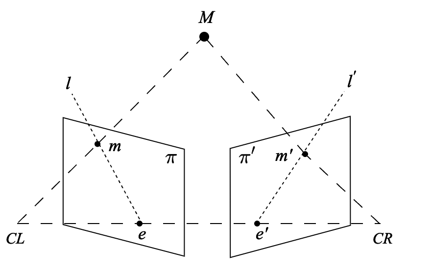
(a)

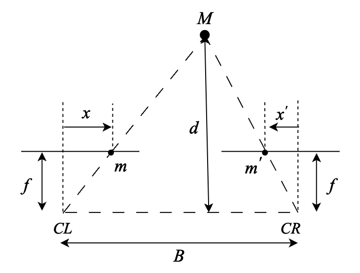
(b)

Figure 1: (a) Epipolar geometry of two cameras. (b) Epipolar geometry of a rectified image pair.

Fig. 1(a) illustrates the epipolar geometry of two pinhole cameras observing a 3D point $\mathbf{M}$. Stereo reconstruction estimates $\mathbf{M}$’s distance by analyzing its projections $\mathbf{m}$ and $\mathbf{m}^{\prime}$. The baseline $B$ connects camera origins $\mathbf{CL}$ and $\mathbf{CR}$, defining epipolar geometry with epipoles $\mathbf{e}$ and $\mathbf{e}^{\prime}$. The epipolar plane intersects with image planes $\boldsymbol{\pi}$ and $\boldsymbol{\pi}^{\prime}$, forming epipolar lines. According to epipolar geometry, $\mathbf{m}$ in $\boldsymbol{\pi}^{\prime}$ lies on epipolar line $l^{\prime}$. Depth estimation involves finding corresponding points, simplified by image rectification in Fig. 1(b), ensuring $\mathbf{m}$ and $\mathbf{m}^{\prime}$ align. Depth $d$ is estimated through triangulation represented by Eq. 1, considering column differences from $\mathbf{m}$ and $\mathbf{m}^{\prime}$ to the center of the left and right images, baseline $B$, focal length $f$, and pixel width $\delta$ in the rectified image sensor.

$$d=\frac{B*f}{\delta*\left(x-x^{\prime}\right)}$$ (1)

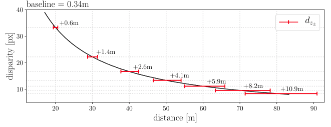
Figure 2: The dependency between depth estimation accuracy and the baseline of the stereo camera design for a baseline, $\mathbf{B}$ of 34cm, based on [10].

Figure 2 shows the theoretical dependency between the baseline parameter of a stereo camera pair and the accuracy of the depth estimates that the stereo sensor will produce. Red lines show the depth deviations associated with a $\pm 1$ pixel error in the disparity. The plot shows that the disparity decreases as a square of the depth and error increases as a square of the depth.

2.2 Mapping Algorithms

This article focuses on the following three representative state-of-the-art algorithms to investigate their applications to UAV-borne mapping:

• Structure-from-Motion: Direct Sparse Odometry (DSO) [5]

• Stereo reconstruction: Direct Sparse Odometry with Stereo Cameras (SDSO) [32] and Direct Sparse Odometry Lite (DSOL) [19]

2.2.1 DSO: Direct Sparse Odometry

DSO is a visual odometry technique that adapts SfM methods for 3D reconstruction. It directly estimates the camera motion and the sparse 3D structure of the environment from a sequence of 2D images by minimizing photometric errors. DSO differs significantly from traditional techniques by directly optimizing photometric errors in images, without relying on keypoint detectors or geometric priors. For a point, $\mathbf{p}$ in reference frame $I_{i}$, observed as $\mathbf{p^{\prime}}$ in target frame $I_{j}$, the photometric error, given by Eq. 2, is formulated as the weighted Sum of Squared Differences (SSD) over a small neighborhood of pixels.

$$E_{\mathbf{p}j}:=\sum_{\mathbf{p}\in\mathcal{N}_{\mathbf{p}}}w_{\mathbf{p}}\left\|\left(I_{j}\left[\mathbf{p}^{\prime}\right]-b_{j}\right)-\frac{t_{j}e^{a_{j}}}{t_{i}e^{a_{i}}}\left(I_{i}[\mathbf{p}]-b_{i}\right)\right\|_{\gamma}$$ (2)

where $\mathcal{N}_{\mathbf{p}}$ is the set of pixels in the SSD; $(t_{i},t_{j})$ the exposure times of the frame $I_{i}$ and $I_{j}$; $(a_{i},b_{i},a_{j},b_{j})$ the brightness transfer variables defined in DSO for frame $I_{i}$ and $I_{j}$ respectively; And $\|\cdot\|_{\gamma}$ is the Huber norm. In addition to using robust Huber penalties, a gradient-dependent weighting $w_{\mathbf{p}}$ is applied. Further, $\mathbf{p}^{\prime}$ stands for the projected point position of $\mathbf{p}$ with inverse depth $d_{\mathbf{p}}$ ,given by

$$\mathbf{p}^{\prime}=\Pi_{\mathbf{c}}\left(\mathbf{R}\Pi_{\mathbf{c}}^{-1}\left(\mathbf{p},d_{\mathbf{p}}\right)+\mathbf{t}\right)$$ (3)

with

$$\left[\begin{array}[]{cc}\mathbf{R}&\mathbf{t}\\ 0&1\end{array}\right]:=\mathbf{T}_{j}\mathbf{T}_{i}^{-1}$$ (4)

where $\mathbf{T}_{i},\mathbf{T}_{j}\in\textbf{SE}(3)$ are the camera poses represented by transformation matrices for frame $I_{i}$ and $I_{j}$.

To minimize the photometric error between the corresponding points in two frames, DSO incorporates a fully direct probabilistic model that jointly optimizes all model parameters, including camera motion and geometry, represented as inverse depth in a reference frame. The optimization is accomplished using the Gauss-Newton algorithm in a sliding window [13].

2.2.2 SDSO: Direct Sparse Odometry with Stereo Cameras

SDSO is a stereo version of DSO. In a monocular mapping system like DSO, to initialize the whole system, i.e., to track the second frame with respect to the initial one using Eq. 2, the inverse depth values $d_{p}$ of the points in the first frame are required. In DSO, the points are initialized to have random depth values ranging from 0 to infinity, corresponding to a large depth variance. Unlike that, SDSO uses stereo matching to estimate a semi-dense depth map for the first frame, which significantly increases the tracking accuracy. The constraints from static stereo introduce scale information into the system. They also provide good geometric priors to temporal multi-view stereo.

2.2.3 DSOL: Direct Sparse Odometry Lite

DSOL presents an enhanced version of DSO and SDSO, proposing several algorithmic and implementation improvements to significantly speed up computation. Key aspects of the methodology include: (1) utilizing an inverse compositional alignment method for frame tracking, improving accuracy and speed. (2) adapting a better stereo photometric bundle adjustment formulation compared to SDSO. (3) Simplifying keyframe creation and removal criteria from DSO, allowing for better utilization of computational resources and parallel processing. (4) Implementing algorithmic enhancements to streamline the computation process, making it more suitable for real-time applications, especially in resource-constrained environments. Compared to DSO and SDSO, the focus of DSOL is on mapping speed and efficiency while maintaining accuracy.

3 Methodology

This section initiates by exploring optimal practices for UAV systems operating in both daytime and nighttime settings, offering a theoretical basis for the selection of sensors. Subsequently, the section delves into detailing the data and metrics employed to assess the efficacy of mapping algorithms in drone applications. Synthetic data was prioritized over real-world data due to its accessibility and the presence of ground truth 3D mapping information. The evaluation primarily centers on appraising the geometric accuracy of the reconstructed map.

3.1 Sensors for UAV Mapping

Three prominent sensor types are investigated as potential components of the UAV perceptual payload. These sensor types are listed below:

• LiDAR (Light Distance and Ranging) Sensors

• Event Cameras

• Conventional EO and IR Cameras

Our assessment considered leading examples of each sensor that would be potentially appropriate for integration and commercially available. The specifications of the sensors were then reviewed in terms of their ability to provide measurements that meet the requirements of UAV mapping. Based on this analysis, a determination was reached regarding the suitability of each sensor.

3.1.1 LiDAR

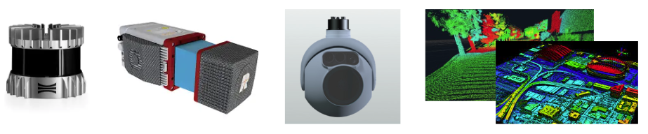
Figure 3: Several LiDAR sensors were evaluated for inclusion on the platform. Left to right are shown the Ouster OS1, the HRL131, the RIEGL miniVUX-HA, and the L3 Harris Tactical Geiger-Mode LiDAR sensors.

Fig. 3 shows several LiDAR sensors evaluated for inclusion in the platform payload. However, it was quickly determined that these devices would not be appropriate for the UAV mapping application. The shortcomings of these sensors are described in the list below:

• Weight: LiDAR sensors typically weigh 500 g. or more which would be equivalent to approximately 5 image sensors of 100g.

• Measurement method: LiDAR sensors measure individual 3D points at one time or a collection of 3D points using a laser line-scanning technology. In either case, a rotating mirror in the sensor scans the scene over time. Accurate integration of scan data requires motion compensation for individual 3D point measurements for mapping and geometry estimation.

• Measurement speed: LiDAR sensors typically scan at low rates (10-20 Hz) which makes the capture of a complete 3D scene geometry impractical for the rates required by high-speed flight.

The data stream, resulting from the combination of the measurement method and measurement speed, requires highly accurate flight pose tracking over long distances at high speeds for the accurate integration of data into a unified 3D map. Achieving this may pose challenges considering the tracking accuracy limitations of onboard instruments, and substantial computation may be required for per-point or per-scan line motion compensation. Due to these reasons, the utilization of LiDAR sensing instrumentation for high-speed UAV mapping is not advisable.

3.1.2 Event Cameras

Fig. 4 shows several event camera sensors evaluated for inclusion in the platform payload. The key attractive aspect of event cameras that has sparked considerable interest from researchers and industry alike is the extremely high temporal accuracy. Specifically, event cameras can resolve intensity changes in the perceptual field at a temporal resolution of approximately $1\mu s$. For this reason, event cameras have been used in high-speed contexts.

While the deployment of event cameras as a component of UAVs may seem attractive due to the temporal resolution, there are several shortcomings associated with integrating this hardware into the UAV payload:

• Resolution: Resolution is a key parameter for depth accuracy as discussed in the stereo reconstruction Sec. 2.1.2. Accuracy strongly ties to both resolution and pixel size, $\delta$, as shown in Fig. 1(b) and Fig. 2. Event camera resolution, 0.3 pixels, is a factor of 5-10 times lower than conventional image sensors, and the pixel size of $\delta=18\mu m$ is a factor of 6-18 times larger than conventional image sensors, e.g., the Sony IMX472 sensor has a resolution of 21 Mpixels and a pixel size of $3.3\mu m$.

• Weight: While these sensors are lighter than LiDAR sensors, they weigh $\sim$100 g. and much lighter camera sensors are available.

• Latency: While the temporal resolution of event cameras is an impressive $1\mu s$, the latency of the measurements is on the order of $<1ms$. This latency is similar to that of high frame rate conventional image sensors with frame rates of +100 fps and similar $<1ms$ latency.

• Nighttime Performance: Event cameras operate on similar principles to conventional visible light cameras. As such, they are suited to deployment in daytime contexts. The lack of an infra-red event camera requires completely separate perceptual software stacks for the vehicle in daytime and nighttime contexts.

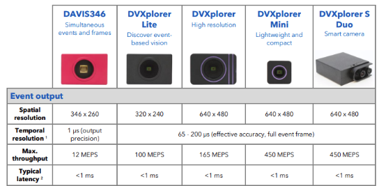
Figure 4: A collection of event cameras commercially available from iniVation Corp.

Event cameras are a recent technology that has emerged and matured over the past decade. These sensors have unparalleled temporal resolution of $1\mu s$ which makes them popular for capturing high-speed phenomena endemic to high vehicle speed applications. Yet, current technology has not matured to the extent required to make this sensor a viable option. Further, the development of a nighttime IR sensing event camera is an active area of sensor development under initiatives with no commercially viable examples. The drawbacks of having low sensor resolution, large pixel size, and no nighttime performance combined with comparable latency and weight to standard conventional cameras suggest that this sensor is not appropriate for inclusion as a component of the UAV payload for high-speed mapping applications.

3.1.3 Conventional EO and IR Cameras

Conventional image sensors have many beneficial attributes that often make them the sensor of choice for perception designs that must satisfy low Size, Weight, and Power (SWaP) requirements. They are well-suited for UAV mapping tasks for several reasons:

• SWaP: Both EO and IR camera modules are available commercially in a very large variety of form factors. This includes a compact 25$mm^{3}$ weighing 10-50g requiring $\sim$1$W$ for power and providing temporally synchronized high framerate (60fps) images.

• High-Quality Imaging: Modern cameras offer high-resolution imaging with the ability to capture fine details, which is crucial for mapping tasks, especially in scenarios where identifying objects is essential.

• Mapping and Geospatial Data: Cameras can be used for aerial imaging and photogrammetry to create detailed maps and 3D models of areas, making them valuable for urban planning, environmental monitoring, and disaster management.

• Stereo Vision: Cameras can be paired to create a stereo vision system. By capturing images from two slightly offset viewpoints, they can calculate depth information through triangulation, using the disparity between corresponding points in the two images. This method provides accurate 3D information.

• Integration with Other Technologies: Cameras can be integrated with other sensors and technologies, such as Inertial Measurement Units (IMUs) and Global Positioning Systems (GPSs), to enhance their capabilities and improve accuracy.

• Wide Field of View: Many cameras have wide-angle lenses or the ability to pan, tilt, and zoom (PTZ), providing a broad field of view and the flexibility to focus on specific areas of interest.

• Daytime and Nighttime Versatility: Camera sensors are capable of sensing in both daylight and nighttime conditions. If high sensitivity is needed in both scenarios, it is possible to replace daytime image sensors with infrared image sensors during nighttime conditions. This can be done with minor modifications to the underlying software and algorithms.

• Large active algorithm ecosystem: Researchers worldwide develop cutting-edge algorithms for these sensors at top institutions. Utilizing this sensor type enables leveraging the latest, optimized, and theoretically advanced algorithms for vehicle perception tasks.

• Cost-Effectiveness: Compared to some other sensing technologies, cameras are cost-effective, making them accessible for a wide range of surveillance and mapping applications.

Conventional image sensors have many beneficial attributes that make these sensors attractive for use as part of the Bumblebee perception payload. These sensors have low SWaP requirements and can record ¿16M measurements at a time from the environment. These sensors can be combined with lens components that provide both wide-angle viewpoints, e.g., a 230^∘ FOV via the fisheye lens, for omnidirectional perception and confined viewpoints, e.g., 80^∘ FOV “standard” lens, for high fidelity target tracking and mapping. The intensive work required to integrate these sensors and develop optimized algorithms to process their data to work using onboard computing resources can be reused between daytime (EO) and nighttime (IR) sensing contexts.

In the realm of image sensors, those designed for both infrared (IR) and visible light often share common image processing algorithms, including basic processes like filtering, noise reduction, contrast enhancement, and image registration. Additionally, object detection, recognition, feature extraction, and image fusion algorithms can typically be adapted for both IR and visible light images, leveraging shared features and patterns. However, notable differences emerge, primarily related to spectral characteristics, illumination, noise, calibration, temperature considerations, environmental conditions, and the unique sensitivities of IR images to object materials. These distinctions necessitate adjustments in algorithms to address variations in contrast, object recognition, and material discrimination, showcasing the need for specialized approaches in certain contexts.

3.2 Benchmark Dataset

A virtual environment that mimics real-world scenes was used for evaluation. Compared to real datasets, synthetic datasets for evaluating mapping algorithms bring a notable advantage in the form of readily available ground truth 3D models. This availability of ground truth data facilitates a more rigorous assessment of mapping performance, ensuring precise comparisons between the algorithm’s outputs and the known true state of the environment.

3.2.1 Environment Simulation

AirSim [22] was used to simulate the dynamics of the drone. AirSim, developed by Microsoft, stands as a groundbreaking and influential simulator that has become a cornerstone in the development of autonomous drones and robotics. What sets AirSim apart is its capacity to simulate complex and dynamic environments with exceptional fidelity, replicating not only the physics of flight but also the intricacies of various sensors like cameras (RGB and depth), LiDAR, and GPS. Fig. 5 is an example of the AirSim simulated images captured by the cameras mounted on the multirotor.

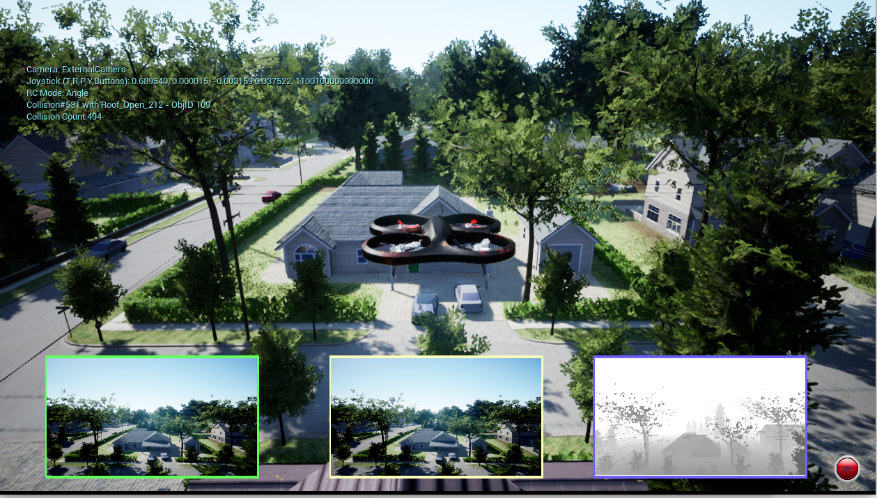
Figure 5: An example of an AirSim environment showing the FPV view (main image) and simulated images at the bottom for cameras including stereo RGB (left and middle) and depth (right).

Although AirSim provides rich virtual environments for testing and fine-tuning a wide array of autonomous systems, these environments are often designed for games and lack realism. To simulate real-world flights and ultimately enhance the authenticity and effectiveness of simulations, this article used the Cesium plugin for the Unreal Engine, also known as “Unreal Cesium”. This plugin creates a powerful combination by integrating the Unreal Engine’s advanced rendering and simulation capabilities with Cesium’s geospatial visualization and data streaming features. By streaming high-resolution 3D models from Google Maps (latitude and longitude location required), overlying them onto real-world maps, and applying dynamic lighting and shadows, to provide precise representations of real-world locations, such as cities, terrains, and 3D models of buildings. This integration allows developers to create highly realistic and geospatially accurate virtual environments for various applications. Once the 3D map is generated, it behaves as a collision object in the Unreal Engine. Unmanned Aerial System (UAS) then interacts with this model using the geometry of the environment and a physics engine. Fig. 6 demonstrates the benefits of the Unreal Cesium plugin for simulation. It shows three real-world locations: (1) the UNC Charlotte campus, USA, (2) the Grand Canyon, USA, and (3) Paris, France.

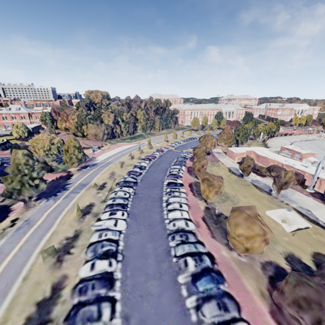
(a) UNC Charlotte, NC, USA

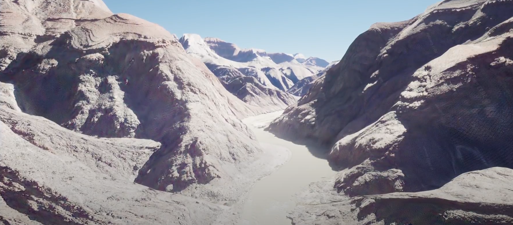
(b) Grand Canyon, AZ, USA

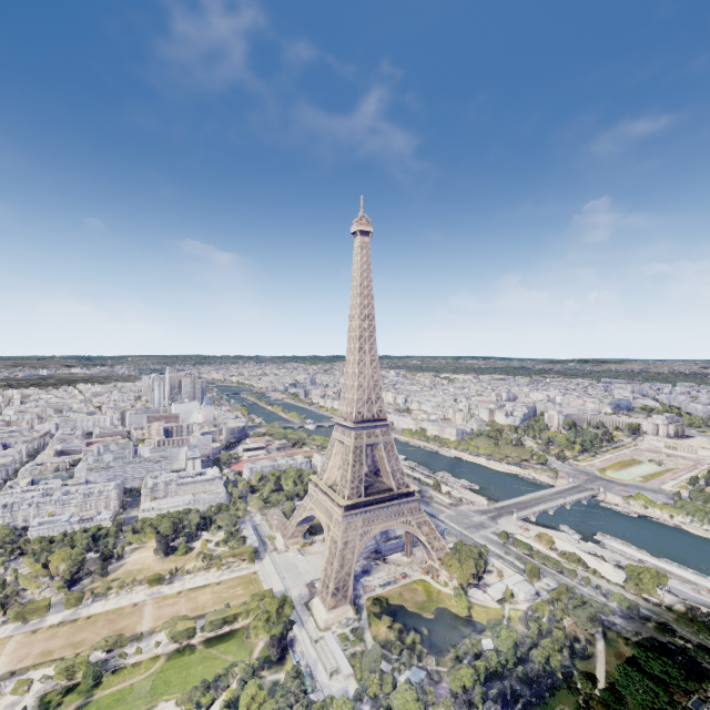
(c) Eiffel Tower, Paris, France

Figure 6: Realistic environments created using Unreal Engine and Cesium Plug-in.

3.2.2 Flight Simulation

Fig. 7 depicts the proposed pipeline for flight simulation. QGroundControl and PX4-Autopilot are software components commonly used in the field of UAVs and drones. They work together to provide a comprehensive solution for controlling and managing drone flights. The missions are planned by defining waypoints, flight paths, and specific actions for the drone to perform and QGroundControl sends the mission plans to the autopilot system PX4-Autopilot. As an open-source flight control software for UAVs, PX4-Autopilot runs on the flight controller onboard the drone and is responsible for stabilizing the aircraft, executing flight plans, and interfacing with sensors and actuators. Controlled by PX4-Autopilot, the simulated UAV in AirSim follows the planned trajectory in a high-realism virtual environment created by Unreal Engine and Cesium plug-in. The cameras mounted on the UAV then capture the images (RGB, depth, etc) of the scene. These images along with the ground truth vehicle odometry can be obtained from AirSim, which can be used to reconstruct the ground truth 3D model of the world.

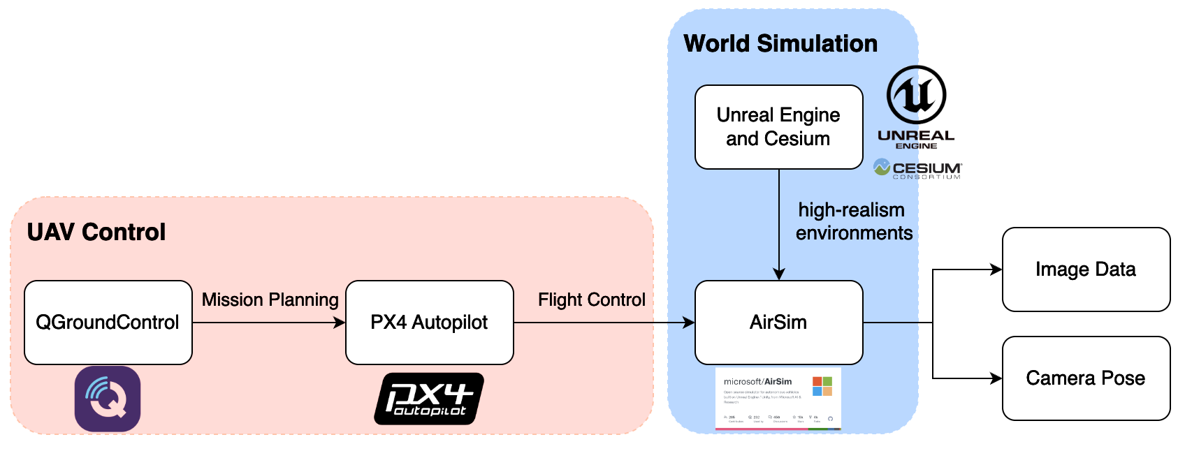
Figure 7: The flight simulation pipeline integrates 4 robot development technologies to facilitate development and testing: (1) Unreal Engine and Cesium Plug-in (high-realism image synthesis), (2) AirSim (vehicle dynamics), (2) QGroundControl (mission planning), and (4) PX4-Autopilot (vehicle control and Software-In-The-Loop).

3.3 Evaluation Methods

The evaluation of mapping performance encompasses two key dimensions: mapping accuracy and mapping speed. Mapping accuracy is meticulously assessed by comparing the geometry of the reconstructed point cloud with the ground truth point cloud. The ground truth point cloud is generated utilizing the accurate odometry and depth data provided in the simulated environment. Prior to the comparison process, the Iterative Closest Point (ICP) algorithm [1] is employed to establish point correspondences, associating points in the reconstructed point cloud with their counterparts in the ground truth cloud. Geometric accuracy serves as a pivotal metric, offering profound insights into the mapping algorithm’s ability to faithfully capture spatial relationships between reconstructed points and their true locations. Conversely, mapping speed quantifies the computational resources required for tracking frames and generating keyframes, which ultimately influences the efficiency of the reconstructed point cloud generation process. This comprehensive evaluation framework contributes to a nuanced understanding of the mapping algorithm’s overall performance, facilitating robust comparisons among different mapping methodologies.

3.3.1 Iterative Closest Point (ICP)

The Iterative Closest Point (ICP) algorithm [1] stands as a widely employed iterative optimization method for aligning two point clouds. Its primary objective is to determine the optimal transformation (comprising rotation, translation, and scale factor) that minimizes the distances between corresponding points in the two point clouds. Commencing with an initial estimate for the transformation, encompassing a scale factor $\mathbf{s}$, a rotation matrix $\mathbf{R}$, and a translation vector $\mathbf{t}$, the algorithm iterates through a sequence of steps. Initially, it establishes point correspondences between the source and target clouds by associating each point in the source with its nearest counterpart in the target. Subsequently, it calculates an error metric by evaluating the squared Euclidean distances among corresponding points. The algorithm then assesses convergence, and if the error falls below a predefined threshold, it terminates; otherwise, it proceeds to refine the transformation to further minimize the error. This iterative refinement process persists until either convergence is achieved or a predetermined maximum iteration count is reached.

3.3.2 Geometric Accuracy

With the correspondences found using the ICP algorithm, the geometric accuracy of the reconstructed map is measured by the distance between corresponding points in the ground truth 3D model and the reconstructed 3D map. Root Mean Square Error (RMSE) is used as a metric of geometric accuracy. RMSE is a measure of the average error between the reconstructed and ground truth positions. It penalizes larger errors more heavily due to the squared term. The equation for calculating RMSE is:

$$RMSE=\sqrt{\frac{1}{N}\sum_{i=1}^{N}\left(\mathbf{P}_{i}-\mathbf{T}_{i}\right)^{2}}$$ (5)

where $N$ is the total number of points in the reconstructed point cloud, $\mathbf{P}_{i}$ is the position of the $i$-th reconstructed point, and $\mathbf{T}_{i}$ is the ground truth (reference) position of the corresponding $i$-th point.

Further, the standard deviation (std) of the errors (distances) is used to evaluate the variability in the errors, calculated as follows:

$$\sigma=\sqrt{\frac{\sum_{i=1}^{N}(x_{i}-\bar{x})^{2}}{N}}$$ (6)

where $\bar{x}$ is the mean of the errors.

4 Results

Simulated experiments were conducted using a virtual model of the UNC Charlotte campus near the football stadium. The virtual model of this environment was generated using the Unreal Engine and the Cesium plug-in. The imaging setup on the simulated multirotor comprised a pair of stereo cameras. For DSO (SfM), only data from the left camera was utilized, while DSOL and SDSO (stereo reconstruction) utilized the stereo data. Additionally, a depth sensor on the multirotor provided ground truth depth information and scene point cloud. The multirotor maintained an average speed of 16.5 m/s, with a maximum horizontal speed of 20 m/s during the flight. Fig. 8(a) illustrates the simulated drone’s flight over the UNC Charlotte football stadium, covering a 3-minute flight duration and capturing 1027 RGB-D frames. Sample images from the drone’s simulated RGB and depth sensors are displayed in Figs. 8(b) and 8(c).

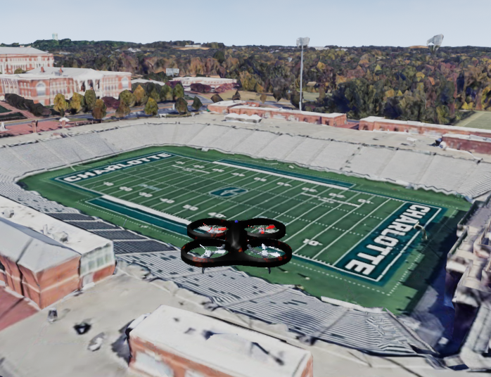
(a) A multirotor flying over a simulated virtual model of UNC Charlotte campus.

(b) A RGB image captured by the drone camera.

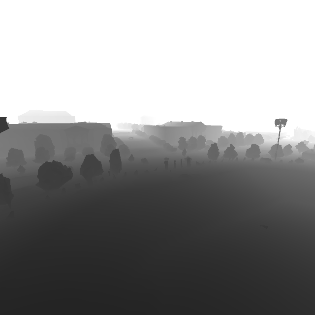
(c) A depth image captured by the drone camera.

Figure 8: A simulated UNC Charlotte campus world.

The experiments were conducted on an Intel i7-12700KF CPU. The official implementation of DSO and DSOL were used for evaluation. An open-source implementation of SDSO [25] based on the official DSO with stereo integration was employed, as no official implementation is available. All implementations adhered to the original configuration with the default parameters.

4.1 Mapping Accuracy Evaluation

The ground truth point cloud of the experimental scene is shown in Fig. 9. This was generated by transforming the point cloud of each RGB-D frame to the location of the multirotor obtained from the ground truth odometry provided by AirSim. This point cloud was used as the ground truth geometry to evaluate the mapping accuracy of different algorithms.

Figure 9: The ground truth point cloud of the scene generated by applying the ground truth odometry to the point cloud of each RGB-D frame.

Fig. 10 shows the point cloud respectively reconstructed by DSO, SDSO, and DSOL. All three maps reflect the experimental scene. However, there are a lot richer structures in both DSO and DSOL maps than in the DSOL map. Detailed analysis is provided in the following sections.

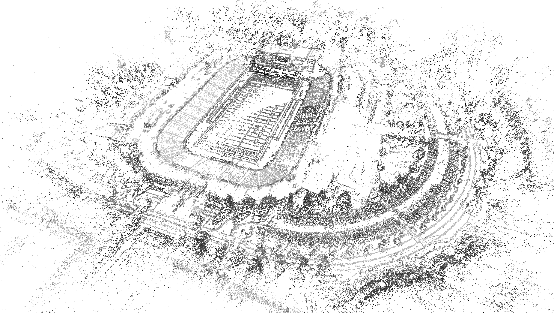
(a) DSO

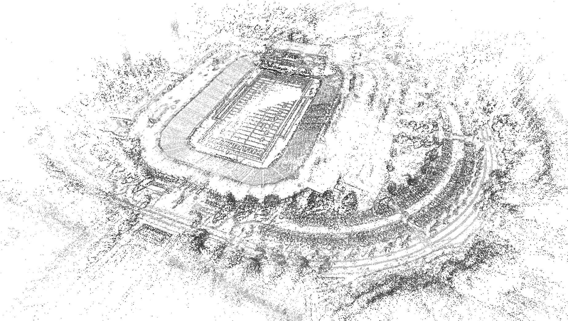
(b) SDSO

(c) DSOL

Figure 10: Point clouds generated by DSO (left), SDSO (middle), and DSOL (right). DSO and SDSO generated much more point clouds than DSOL. The color of the points is represented by the grayscale color of the scene point.

4.1.1 Quantitative Analysis

	GT	DSO	SDSO	DSOL
points	236032175	204345	212179	6662
correspondences	-	172862	175567	2670
map scale	-	35.98	1.01	1.11
RMSE	-	0.155	0.164	0.229
std	-	0.110	0.114	0.141

Table 1: Mapping accuracy of three mapping algorithms. DSO and SDSO maps contain $\sim$30$\times$ more points than the DSOL map. The map scales are obtained by estimating the scale factor from the reconstructed point cloud to the ground truth. DSO, as a monocular mapping algorithm, is not able to correctly estimate the scale of the map.

Table 1 details the density and accuracy characteristics of mapping results obtained from different algorithms. In our experimental setup, we utilized the Iterative Closest Point (ICP) algorithm to align the reconstructed point clouds (source) with the ground truth point cloud (target). The specified search radius, representing the distance from each point in the source point cloud within which the ICP algorithm seeks a corresponding point in the target point cloud, is set at 0.5 meters. Once all correspondences are established, the scale factor from the source to the target point cloud, along with the fitting error, can be derived. The “GT” column provides information about the ground truth point cloud, while the three subsequent columns present statistics related to the reconstructed point clouds. Notably, DSO and SDSO maps encompass approximately 30 times more points than the DSOL map, aligning with the observations in Fig. 10. The contrast in the correspondence sets is more pronounced, with DSO and SDSO revealing approximately 65 times more correspondences than DSOL. The “map scale” reflects the scale factor from the reconstructed point cloud to the ground truth, with DSO unable to accurately estimate scale as a monocular mapping algorithm. The increased number of correspondences likely provides a more robust basis for establishing the scale between the reconstructed point cloud and the ground truth, resulting in a more accurate map scale for SDSO. The “RMSE” and “std” rows, namely the Root Mean Square Error and standard deviation, reveal noteworthy distinctions in accuracy and consistency. DSO exhibits the lowest RMSE (0.155) and a small std (0.110), indicating both high accuracy and consistency. SDSO follows closely with an RMSE of 0.164 (5.81% higher) and a comparable std of 0.114 (3.64% higher). In contrast, DSOL demonstrates a higher RMSE of 0.229 (47.74% higher than DSO and 39.63% than SDSO) and a larger std of 0.141 (28.18% higher than DSO and 23.68% than SDSO), suggesting lower accuracy and greater variability. While DSO and SDSO prove more accurate and consistent in their mapping results, DSOL lags in terms of both precision and reliability.

Fig. 11 further characterizes the mapping accuracy of three algorithms with the histogram of the distance between found matched points. As shown in the figure, most matched points in DSO and SDSO are within 0.15$m$ distance from their correspondences in the ground truth point cloud. In contrast, DSOL has much fewer points than are within this distance range and more points that have a distance greater than 0.2$m$. This histogram further supports the conclusion about mapping accuracy in Table 1.

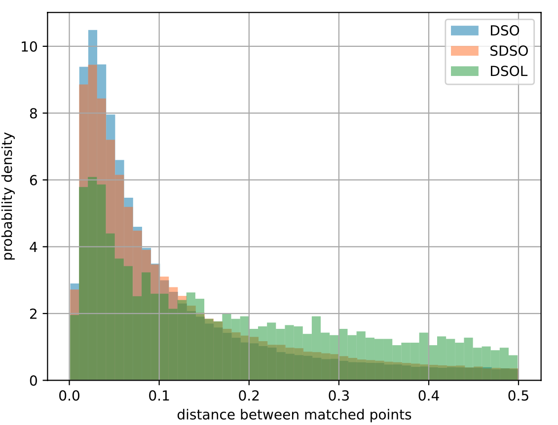
Figure 11: The histogram of the fitting error. The error is measured as the distance from the points reconstructed by mapping algorithms to their corresponding points in the ground truth point cloud.

The examination of reconstruction accuracy concerning point depth is elucidated in Fig. 12. The depth distribution of matched points within the reconstructed maps is delineated in Fig. 12(a). It can be seen that across all three mapping algorithms, points with depths ranging from 20$m$ to 60$m$ predominate, constituting approximately 50% of the total points. Fig. 12(b) portrays the reconstruction RMSE across distinct depth ranges. The discernibly higher values and sparsity of points further substantiate the assertion that the reconstructed map by DSOL exhibits inferior accuracy and reliability compared to those produced by DSO and SDSO. At distance of 20-40$m$, the reconstruction error of DSOL is approximately 0.2$m$ per point while DSO and SDSO are close to each other having an approximately 0.13$m$ point-wise fitting error. Beyond a depth of 60$m$, DSO outperforms SDSO with a slightly smaller fitting error. Additionally, the error distribution of three maps underscores an observed quadratic relationship, wherein mapping errors escalate as point depth increases. An anomaly occurs on the leftmost side of the figure, where all three algorithms display elevated fitting errors (DSO and SDSO point are overlapped with each other). This phenomenon is attributed to the limited number of points within the 10$m$ range, as evident in Fig. 12(a). The scarcity of samples within this range hinders a comprehensive representation of fitting errors.

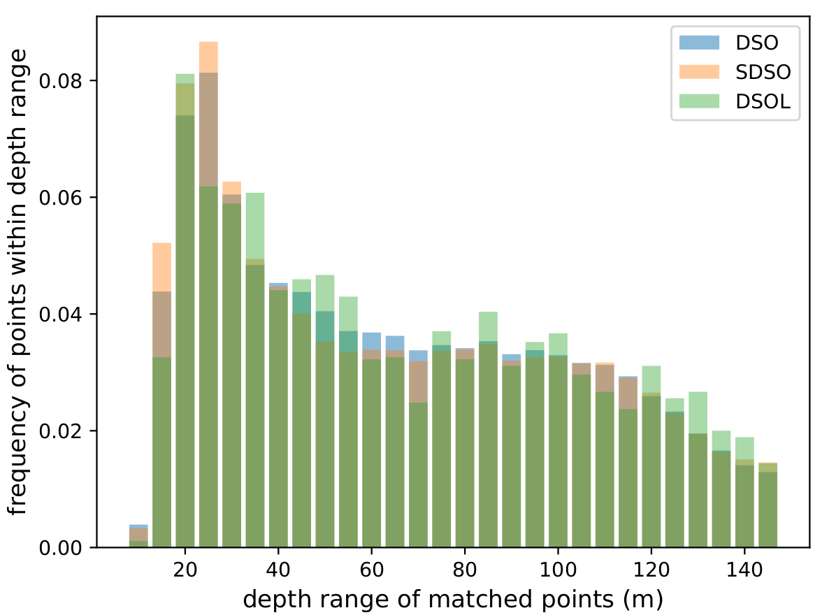
(a)

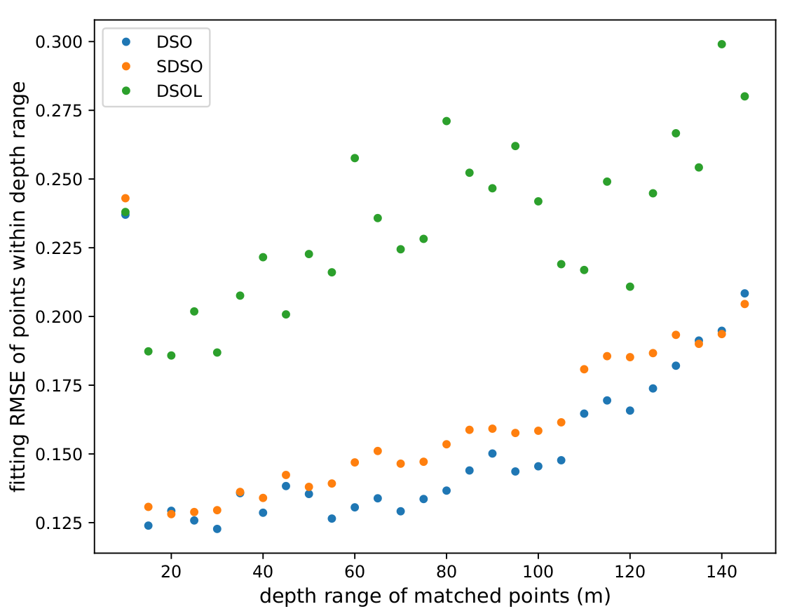
(b)

Figure 12: Distribution of point depth in the reconstructed maps (left) and reconstruction RMSE of points at different depth ranges (right).

4.1.2 Qualitative Analysis

A qualitative examination of the reconstructed maps from DSO, SDSO, and DSOL, as illustrated in 13, unveils notable distinctions in their alignment with the ground truth. DSO and SDSO, with their significantly higher point densities, exhibit commendable accuracy in capturing the details of the road network, showcasing intricate and well-aligned representations. The enhanced point density, particularly evident in the football stadium region, allows for a more detailed reconstruction, resulting in superior alignment with the ground truth in this specific area. Conversely, DSOL, characterized by a sparser point cloud, displays a more conservative reconstruction, which translates into a reduced level of detail, particularly in complex structures like the football stadium. Although DSOL shows commendable alignment on the roads, its limitations in point density become apparent in areas with more intricate features.

(a) DSO

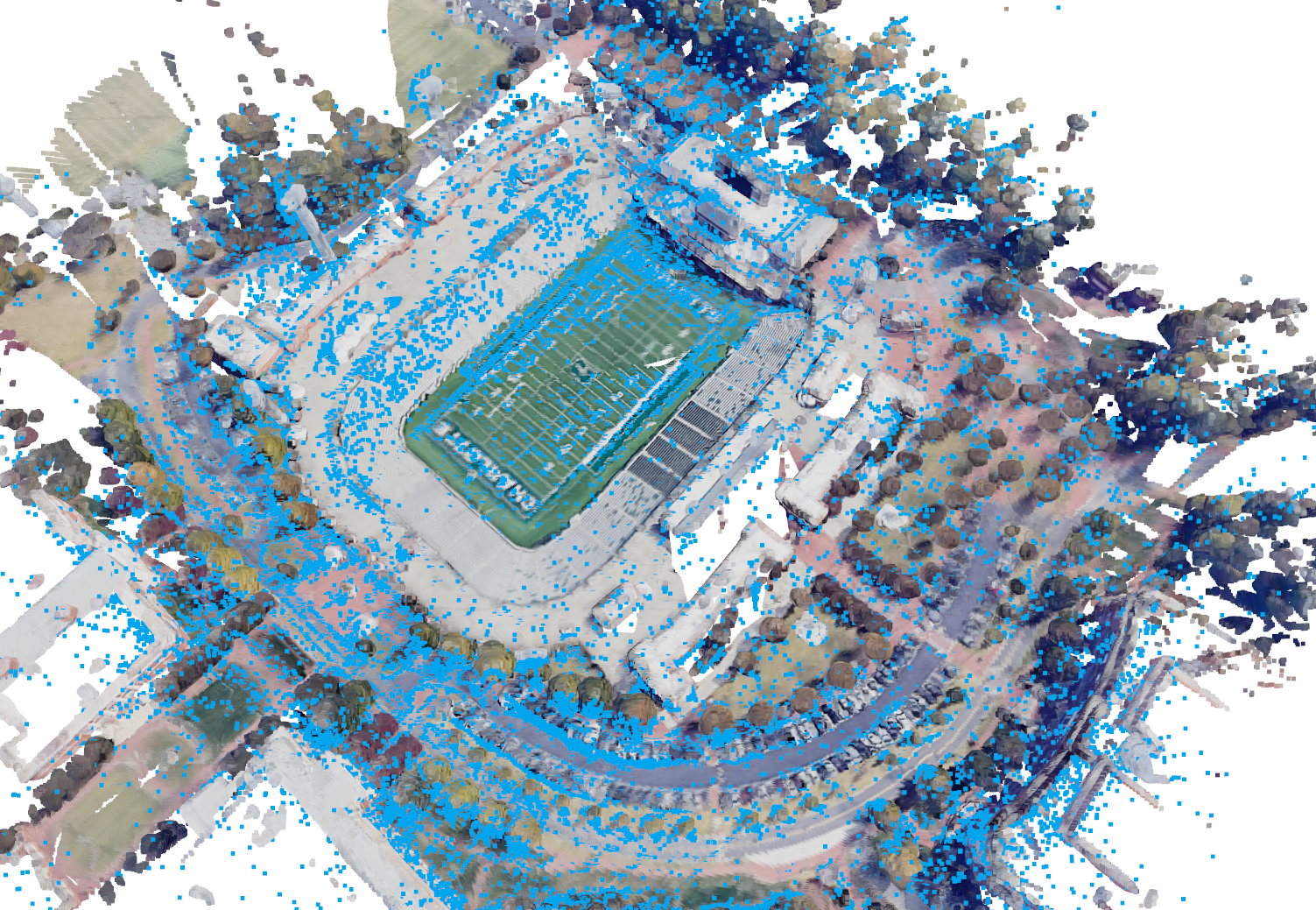
(b) SDSO

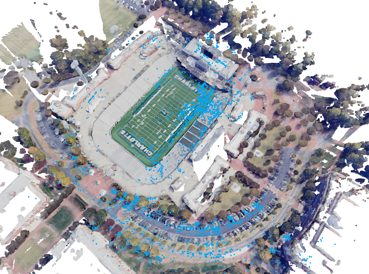
(c) DSOL

Figure 13: Reconstructed point clouds (blue) overlaid with the ground truth point cloud (actual color): DSO (left), SDSO (middle), and DSOL (right). All three reconstructed point clouds have been scaled by the factors in Table. 1.

4.2 Computational Cost Evaluation

This section is dedicated to a comprehensive examination of the computational cost exhibited by the three mapping algorithms. The effectiveness of these algorithms is scrutinized with a particular focus on two critical aspects of mapping computational cost: keyframe creation time and frame tracking time. These metrics serve as crucial benchmarks in assessing the algorithms’ ability to swiftly and accurately generate keyframes, as well as tracking real-time camera pose changes during the mapping process. Through this meticulous examination, we seek to offer valuable insights that contribute to the informed selection and deployment of mapping solutions across a spectrum of real-world applications.

4.2.1 Keyframe Creation Time

Fig. 14 illustrates the keyframe creation time for DSO, SDSO, and DSOL. It can be seen that SDSO requires the most time in creating a keyframe, averaging $\sim$220.73$ms$ per keyframe, as also reported in Table 2. DSO, benefiting from its exclusion of stereo depth estimation in the mapping process, incurs a comparatively lower computational cost, averaging around $\sim$200.28$ms$ per keyframe. DSOL, characterized by a simplified keyframe creation process and the parallel utilization of available computational resources, demands a notably reduced time of $\sim$7.39$ms$ per keyframe. The columns in Table 2 delineate the statistical distribution of keyframe creation times, including the minimum, maximum, and mean values, with the “std” column denoting the standard deviation. In summary, SDSO necessitates 10.21% more keyframe creation time than DSO and 2886.87% more than DSOL, while DSO requires 2610.15% more time than DSOL.

The “total kfs” column in Table 2 provides insights into the aggregate number of keyframes generated by the three algorithms. DSOL, employing a simplified keyframe creation criterion, notably generates approximately $\sim$80% fewer keyframes compared to its counterparts. Noteworthy is the observation that DSO creates 29 fewer keyframes than SDSO. This discrepancy is attributed to a delayed initialization of the DSO system, commencing at the 50${}^{\text{th}}$ frame in our experiments, in contrast to the immediate initialization of SDSO and DSOL. Such delay is also illustrated in Fig. 14 as the DSO curve starts later than SDSO and DSOL. DSO system’s initialization process relies on assigning random depth values to candidate points and predicting the initial camera movement pattern, demanding precise assumptions about initial depth values and camera motion. In contrast, mapping systems employing stereo cameras, such as SDSO and DSOL, leverage stereo matching for enhanced depth initialization, leading to increased accuracy. The divergence in keyframe quantities among the algorithms also mirrors the disparities in point cloud density depicted in Fig. 10, given that these points are derived from the keyframes.

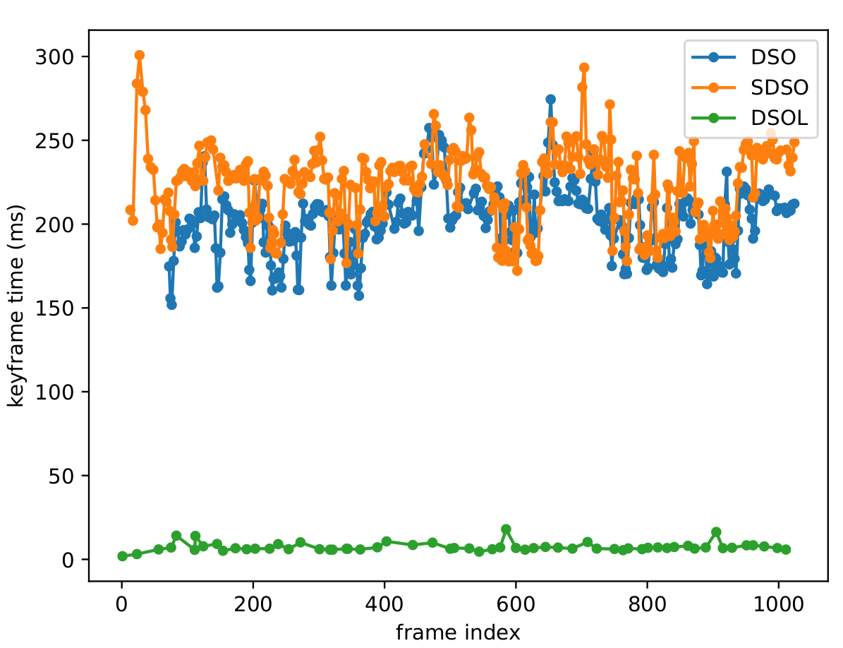
Figure 14: The points plotted along the curves represent the keyframe creation time at each frame. Stereo DSO (SDSO) exhibits a higher temporal requirement than monocular DSO, demonstrating significantly greater computational overhead than DSO-Lite (DSOL). The density of points on the curves serves as a visual indicator of the number of keyframes generated, revealing that both DSO and SDSO produce a larger quantity of keyframes than DSOL.

	total kfs	min ($ms$)	max ($ms$)	mean ($ms$)	std
DSO	330	151.83	274.44	200.28	19.63
SDSO	359	172.19	300.79	220.73	23.08
DSOL	61	1.88	17.99	7.39	2.66

Table 2: Statistics of the keyframe creation results of three mapping algorithms. The “total kfs” column shows the total amount of the keyframes created by three algorithms. The “min”, “max”, and “mean” respectively show the minimum, maximum, and average time for keyframe creation. The “std” column denotes the standard deviation of the keyframe creation time.

4.2.2 Frame Tracking Time

Figure 15 depicts the frame tracking time across various algorithms, employing scatter points for optimal visualization. In the case of DSO and DSOL, the tracking time is stratified into two distinct sections. The upper section, requiring approximately $\sim$60$ms$ for tracking, corresponds to keyframes, while the lower section, with an average tracking time of $\sim$20$ms$ per frame, pertains to non-keyframes. This substantial $3\times$ difference in tracking time arises from the creation of a new keyframe, where all active points are projected onto it with a slight dilation, forming a semi-dense depth map. Subsequent frames are then exclusively tracked to this keyframe, employing traditional two-frame direct image alignment methods. This stratification in tracking time offers insights into the computational demands associated with keyframe and non-keyframe tracking, highlighting the intricacies involved in maintaining accurate and efficient tracking across consecutive frames.

Within the lower section of DSO and DSOL, a further subdivision into two bands is observed. The higher band characterizes the tracking time for frames immediately succeeding keyframes, while the lower band denotes the tracking time for other frames. Notably, the frame following the keyframe requires $\sim$5$ms$ more to track than subsequent frames for both DSO and SDSO. A detailed examination of this behavior, occurring at frame indices 290$\sim$310, is presented on the right side of Fig. 15. This variance in tracking time could be attributed to the fact that the frame following the keyframe typically possesses more feature points that can be projected onto the keyframe, thereby necessitating slightly more time for tracking due to the increased correspondences in the keyframe.

Figure 15: Frame tracking time of different algorithms. The left figure shows the tracking time for all frames including keyframes and non-keyframes. The right figure provides a close-up of the DSO and SDSO tracking time for frames 290$\sim$310. The data is plotted as scatter points for a clear visualization.

5 Conclusions

This study delved into the context of canopy-level and high-speed drone applications. A thorough examination of various sensors underscored their unique strengths and challenges, guiding the selection of suitable devices for specific operational scenarios. The experiments centered on evaluating three prominent mapping algorithms—DSO, SDSO, and DSOL—in a simulated environment, providing valuable insights into the performance of these mapping algorithms. Each algorithm exhibits unique strengths and trade-offs, catering to specific requirements in UAV-based mapping scenarios. DSO, operating as a monocular mapping algorithm, demonstrates versatility in capturing scenes with a single camera, albeit with limitations in scale estimation. SDSO, incorporating stereo depth perception, excels in accuracy and spatial fidelity, as evidenced by its superior point cloud density and detailed reconstructions, particularly in complex structures like the football stadium. On the other hand, DSOL, designed for efficiency, streamlines the mapping process, offering reliable reconstructions with reduced computational demands. The findings emphasize the importance of algorithm selection based on the specific needs of UAV-borne mapping applications, considering factors such as scale estimation, spatial accuracy, and computational efficiency. Future work may involve refining these algorithms for optimized performance in diverse environments, ultimately contributing to advancements in UAV-based mapping for canopy-level and high-speed drone applications. This study contributes to the ongoing discourse on mapping algorithms, providing valuable insights for researchers and practitioners navigating the dynamic landscape of UAV applications in remote sensing and environmental monitoring.

References

- [1] Paul J Besl and Neil D McKay “Method for registration of 3-D shapes” In Sensor fusion IV: control paradigms and data structures 1611, 1992, pp. 586–606 Spie
- [2] Teng Cao, Zhi-Yu Xiang and Ji-Lin Liu “Perception in disparity: An efficient navigation framework for autonomous vehicles with stereo cameras” In IEEE Transactions on Intelligent Transportation Systems 16.5 IEEE, 2015, pp. 2935–2948
- [3] Kurt Cornelis, Marc Pollefeys and Luc Van Gool “Tracking based structure and motion recovery for augmented video productions” In Proceedings of the ACM symposium on Virtual reality software and technology, 2001, pp. 17–24
- [4] David J Crandall, Andrew Owens, Noah Snavely and Daniel P Huttenlocher “SfM with MRFs: Discrete-continuous optimization for large-scale structure from motion” In IEEE transactions on pattern analysis and machine intelligence 35.12 IEEE, 2012, pp. 2841–2853
- [5] Jakob Engel, Vladlen Koltun and Daniel Cremers “Direct sparse odometry” In IEEE transactions on pattern analysis and machine intelligence 40.3 IEEE, 2017, pp. 611–625
- [6] Carlos Hernández Esteban and Francis Schmitt “Silhouette and stereo fusion for 3D object modeling” In Computer Vision and Image Understanding 96.3 Elsevier, 2004, pp. 367–392
- [7] Andreas Geiger, Julius Ziegler and Christoph Stiller “Stereoscan: Dense 3d reconstruction in real-time” In 2011 IEEE intelligent vehicles symposium (IV), 2011, pp. 963–968 Ieee
- [8] Donald B Gennery “A Stereo Vision System for an Autonomous Vehicle.” In IJCAI, 1977, pp. 576–582
- [9] Richard Hartley and Andrew Zisserman “Multiple view geometry in computer vision” Cambridge university press, 2003
- [10] Patrick Irmisch “Camera-based distance estimation for autonomous vehicles”, 2017
- [11] Arnold Irschara, Christopher Zach, Jan-Michael Frahm and Horst Bischof “From structure-from-motion point clouds to fast location recognition” In 2009 IEEE Conference on Computer Vision and Pattern Recognition, 2009, pp. 2599–2606 IEEE
- [12] Olga Krutikova, Aleksandrs Sisojevs and Mihails Kovalovs “Creation of a depth map from stereo images of faces for 3D model reconstruction” In Procedia Computer Science 104 Elsevier, 2017, pp. 452–459
- [13] Stefan Leutenegger et al. “Keyframe-based visual–inertial odometry using nonlinear optimization” In The International Journal of Robotics Research 34.3 SAGE Publications Sage UK: London, England, 2015, pp. 314–334
- [14] Manolis IA Lourakis and Antonis A Argyros “SBA: A software package for generic sparse bundle adjustment” In ACM Transactions on Mathematical Software (TOMS) 36.1 ACM New York, NY, USA, 2009, pp. 1–30
- [15] Benjamin U Meinen and Derek T Robinson “Mapping erosion and deposition in an agricultural landscape: Optimization of UAV image acquisition schemes for SfM-MVS” In Remote Sensing of Environment 239 Elsevier, 2020, pp. 111666
- [16] Jonathan Mooser, Suya You, Ulrich Neumann and Quan Wang “Applying robust structure from motion to markerless augmented reality” In 2009 Workshop on Applications of Computer Vision (WACV), 2009, pp. 1–8 IEEE
- [17] Tudor Nicosevici and Rafael Garcia “Online robust 3D mapping using structure from motion cues” In OCEANS 2008-MTS/IEEE Kobe Techno-Ocean, 2008, pp. 1–7 IEEE
- [18] Sudeep Pillai, Srikumar Ramalingam and John J Leonard “High-performance and tunable stereo reconstruction” In 2016 IEEE International Conference on Robotics and Automation (ICRA), 2016, pp. 3188–3195 IEEE
- [19] Chao Qu, Shreyas S Shivakumar, Ian D Miller and Camillo J Taylor “Dsol: A fast direct sparse odometry scheme” In 2022 IEEE/RSJ International Conference on Intelligent Robots and Systems (IROS), 2022, pp. 10587–10594 IEEE
- [20] Eric Royer, Maxime Lhuillier, Michel Dhome and Jean-Marc Lavest “Monocular vision for mobile robot localization and autonomous navigation” In International Journal of Computer Vision 74.3 Springer, 2007, pp. 237–260
- [21] Grant Schindler, Panchapagesan Krishnamurthy and Frank Dellaert “Line-based structure from motion for urban environments” In Third International Symposium on 3D Data Processing, Visualization, and Transmission (3DPVT’06), 2006, pp. 846–853 IEEE
- [22] Shital Shah, Debadeepta Dey, Chris Lovett and Ashish Kapoor “AirSim: High-Fidelity Visual and Physical Simulation for Autonomous Vehicles” In Field and Service Robotics, 2017 URL: https://arxiv.org/abs/1705.05065
- [23] Sudipta N Sinha et al. “Interactive 3D architectural modeling from unordered photo collections” In ACM Transactions on Graphics (TOG) 27.5 ACM New York, NY, USA, 2008, pp. 1–10
- [24] Minas Spetsakis and John Yiannis Aloimonos “A multi-frame approach to visual motion perception” In International Journal of Computer Vision 6.3 Springer, 1991, pp. 245–255
- [25] “Stereo Direct Sparse Odometry Non-official Implementation” Accessed: 2024-01-02, https://github.com/JiatianWu/stereo-dso
- [26] Danail Stoyanov, Marco Visentini Scarzanella, Philip Pratt and Guang-Zhong Yang “Real-time stereo reconstruction in robotically assisted minimally invasive surgery” In Medical Image Computing and Computer-Assisted Intervention–MICCAI 2010: 13th International Conference, Beijing, China, September 20-24, 2010, Proceedings, Part I 13, 2010, pp. 275–282 Springer
- [27] Richard Szeliski “Computer vision: algorithms and applications” Springer Nature, 2022
- [28] Richard Szeliski and Sing Bing Kang “Recovering 3D shape and motion from image streams using nonlinear least squares” In Journal of Visual Communication and Image Representation 5.1 Elsevier, 1994, pp. 10–28
- [29] Carlo Tomasi and Takeo Kanade “Shape and motion from image streams under orthography: a factorization method” In International journal of computer vision 9 Springer, 1992, pp. 137–154
- [30] Bill Triggs, Philip F McLauchlan, Richard I Hartley and Andrew W Fitzgibbon “Bundle adjustment—a modern synthesis” In Vision Algorithms: Theory and Practice: International Workshop on Vision Algorithms Corfu, Greece, September 21–22, 1999 Proceedings, 2000, pp. 298–372 Springer
- [31] Darren Turner, Arko Lucieer and Christopher Watson “An automated technique for generating georectified mosaics from ultra-high resolution unmanned aerial vehicle (UAV) imagery, based on structure from motion (SfM) point clouds” In Remote sensing 4.5 Molecular Diversity Preservation International (MDPI), 2012, pp. 1392–1410
- [32] Rui Wang, Martin Schworer and Daniel Cremers “Stereo DSO: Large-scale direct sparse visual odometry with stereo cameras” In Proceedings of the IEEE International Conference on Computer Vision, 2017, pp. 3903–3911