Procedure for Obtaining the Analytical Distribution Function of Relaxation Times for the Analysis of Impedance Spectra using the Fox $H$-function

Abstract

The interpretation of electrochemical impedance spectroscopy data by fitting it to equivalent circuit models has been a standard method of analysis in electrochemistry. However, the inversion of the data from the frequency domain to a distribution function of relaxation times (DFRT) has gained considerable attention for impedance data analysis, as it can reveal more detailed information about the underlying electrochemical processes without requiring a priori knowledge. The focus of this paper is to provide a general procedure for obtaining analytically the DFRT from an impedance model, assuming an elemental Debye relaxation model as the kernel. The procedure consists of first representing the impedance function in terms of the Fox $H$-function, which possesses many useful properties particularly that its Laplace transform is again an $H$-function. From there the DFRT is obtained by two successive iterations of inverse Laplace transforms. In the passage, one can easily obtain an expression for the response function to a step excitation. The procedure is tested and verified on some known impedance models.

Keywords: Fox $H$-function; distribution of relaxation time; impedance spectroscopy.

I Introduction

Electrochemical impedance spectroscopy (EIS) is one of the principal techniques used in electrochemistry. EIS data are acquired by applying a small amplitude voltage $v(t)$ (or current $i(t)$) perturbation at different frequencies to an electrochemical system, and measuring the resulting current (or voltage). Applying small magnitude perturbations is meant to suppress nonlinear behaviors, allowing the system to be studied using relatively simple linear models. The impedance (or admittance) spectrum is then defined as the point-by-point ratio between the voltage and the current, both expressed in the frequency domain, i.e. $V(s)$ and $I(s)$ ($s=i\omega$). Note that $V(s)$ and $I(s)$ are the Laplace transforms (LT) of $v(t)$ and $i(t)$, knowing that the LT of a function $f(t)\;(t\in\mathbb{R}^{+})$ is defined by $\mathcal{L}[f(t);s]=F(s)=\int_{0}^{\infty}e^{-st}f(t)dt,\;s\in\mathbb{C}$ and the inverse LT of $F(s)$ is defined by $\mathcal{L}^{-1}[F(s);t]=f(t)={(2\pi i)^{-1}}\int_{\gamma-i\infty}^{\gamma+i\infty}e^{st}F(s)ds,\;\mathcal{R}e(s)=\gamma$. The impedance of a system is thus the complex-valued function Barsoukov and Macdonald (2018); Lasia (2014):

$$Z(f)=\frac{V(s)}{I(s)}=Z^{\prime}(s)+jZ"(s)$$ (1)

which can be used, in principle, to characterize and extract valuable physical, chemical and electrical information about the system under study (e.g. charge transport and transfer processes, charge storage, aging and degradation Barsoukov and Macdonald (2018); Lasia (2014) in batteries Single, Horstmann, and Latz (2019); Bredar et al. (2020); Vadhva et al. (2021), supercapacitors Allagui et al. (2016), fuel cells He and Mansfeld (2009), solar cells Guerrero, Bisquert, and Garcia-Belmonte (2021), electrochemical sensors Pejcic and De Marco (2006), corroding surfaces Mansfeld (1990), biomaterials Cesewski and Johnson (2020); Lisdat and Schäfer (2008), etc.). In this regard, the success of EIS as a useful technique is contingent on the ability of one to describe the system via a quantitative physical model, but this may not often be possible Effendy, Song, and Bazant (2020).

The interpretation of EIS data is commonly done via its (complex nonlinear least squares) fitting to electrical models consisting of resistors, capacitors, inductors, fractional capacitors and fractional inductors arranged in series and/or parallel combinations Bredar et al. (2020). However, this may not always represent the actual physics of the system because the selection of an equivalent circuit is based on the user’s experience and prior understanding of the system Ciucci and Chen (2015). Furthermore, multiple equivalent circuits can actually fit the same data equally well. The data fitting problem can be seen differently if Eq. 1, is rewritten in the time domain with the use of the convolution theorem as Allagui and Fouda (2021); Allagui, Elwakil, and Fouda (2021):

$$v(t)=(z\circledast i)(t)=\int\limits_{-\infty}^{+\infty}z(\xi)i(t-\xi)d\xi$$ (2)

The time-domain function $z(t)$, being the inverse LT of $Z(s)$, represents the collective electrical response to whatever changes are happening from within the system of physical and chemical nature.

If $z(t)$ is considered to be an average relaxation function such that when a current impulse is subjected onto the system the resulting voltage will relax monotonically to zero, we can write $z(t)$ as Ciucci and Chen (2015):

$$z_{D}(t)=c_{0}\delta(t)+\sum\limits_{n=1}^{N}{c_{n}}\theta(t)\tau_{n}^{-1}{e^{-t/\tau_{n}}}$$ (3)

where $\theta(t)$ is the Heaviside theta function, equal to $0$ for $t<0$ and $1$ for $t>0$, $c_{n}\;(n=0,1,\ldots,N)$ are constant coefficients, and $\tau_{n}$ are positive time constants. The term $c_{0}\delta(t)$ represents the response of the system at $t=0$. It is understood that Eq. 3 is obtained by considering the system under test to be of capacitive nature, and comprised of an infinite series of $RC$ elements according to the Debye circuit model. We consider from now on that the impedance function is normalized with respect to an arbitrary resistance $R$.

By taking the LT of Eq. 3 we obtain the impedance of the system in the frequency domain as:

$$Z_{D}(s)=c_{0}+\sum\limits_{n=1}^{N}\frac{c_{n}}{1+s\tau_{n}}$$ (4)

With $c_{0}=R_{0}/R$ being a normalized ohmic resistance, $c_{n}=g_{n}\Delta\tau$ ($\Delta\tau\to 0$), $N\to\infty$, we rewrite the impedance in Eq. 4 as:

$$Z_{D}(s)\approx R_{0}/R+\int\limits_{0}^{\infty}\frac{g(\tau)}{1+s\tau}d\tau$$ (5)

or, as usually preferred with $\gamma(\ln\tau)=\tau g(\tau)$, as

$$Z_{D}(s)\approx R_{0}/R+\int\limits_{0}^{\infty}\frac{\gamma(\ln\tau)}{1+s\tau}d\ln\tau$$ (6)

Here in $Z_{D}(s)$ the frequency is the independent variable, while $R_{0}$ and the distribution function of relaxation times (DFRT) $g(\tau)$ are the unknown model parameters Effendy, Song, and Bazant (2020). We note that the time-domain function $z_{D}(t)$ in Eq. 3 can also be expressed as the integral of exponential decays as follows:

$$z_{D}(t)=(R_{0}/R)\,\delta(t)+\int\limits_{0}^{\infty}{g(\tau)}\theta(t){\tau^{-1}}e^{-t/\tau}d\tau$$ (7)

The elementary Debye kernel in Eq.5 representing an exponential relaxation process can be replaced with other functions. For example, Florsch, Revil, and Camerlynck Florsch, Revil, and Camerlynck (2014) considered the Havrilliak-Negami (HN) model as a kernel. This gives by superposition the following expression for the impedance function:

$$Z_{HN}(s)\approx R_{0}+\int\limits_{0}^{\infty}\frac{g(\tau)}{(1+(s\tau)^{\alpha})^{\beta}}d\tau\quad(0<\alpha,\beta\leqslant 1)$$ (8)

in which the problem is now to retrieve $g(\tau)$ assuming $\alpha$ and $\beta$ are known a priori. It is clear that for $\beta=1$ we recover the Cole-Cole model, with $\alpha=1$ the Davidson-Cole model is recovered, and with $\alpha=\beta=1$ we retrieve back the Debye model.

The aim of this work is to provide a general procedure for recovering analytically the function $g(\tau)$ from Eq. 5 with the use of Fox’s $H$-function and its properties (Section II.2). We note that finding the distribution of the relaxation times can be directly obtained from the experimentally-measured spectral data (i.e. without the need to model it) via numerical inversion methods, such as by Fourier transform techniques Schichlein et al. (2002); Boukamp (2015), Tikhonov regularization Gavrilyuk, Osinkin, and Bronin (2017); Paul et al. (2021); Shanbhag (2020), Max Entropy Hörlin (1998, 1993), genetic algorithm Tesler et al. (2010), etc. Boukamp (2020); Effendy, Song, and Bazant (2020); Liu and Ciucci (2020); Ciucci and Chen (2015). However, it is also instructive to have the analytical expression for the DFRT associated with a given impedance model. For this purpose, we shall first recall from the general treatment of Macdonald and Brachman Macdonald and Brachman (1956) on integral transforms in linear systems some of the useful relations to be used for this analysis (Section II.1). The authors provided there a comprehensive set of relations between the various complex functions used to describe networks and systems, as well as between responses to various types of inputs. These functions can be for instance an impedance or an admittance, a transfer ratio, a complex susceptance, etc. Macdonald and Brachman (1956). Next, after presenting the proposed method of inversion from Eq. 5 with the use of the $H$-function (Section II.2), we derive analytical expressions pertinent to systems described with some of the most widely used models of impedance (Section III).

II Theory

II.1 Basic relations

Using the definitions and notations of Macdonald and Brachman, we define from Eq. 5 the integral transform:

$$Q(s)=\int\limits_{0}^{\infty}\frac{g(\tau)}{1+s\tau}d\tau$$ (9)

as the reduced impedance function for the simple Debye dispersion model $(1+s\tau)^{-1}$. If we define an inverse time constant $\lambda=\tau^{-1}$, and a distribution $D(\lambda)$ as

$$D(\lambda)=\lambda^{-1}g(\lambda^{-1})$$ (10)

then $Q(s)$ in Eq. 9 becomes the iterated LT of $D(\lambda)$ as Macdonald and Brachman (1956):

$$Q(s)=\int\limits_{0}^{\infty}\frac{D(\lambda)}{s+\lambda}d\lambda=\mathcal{L}\{\mathcal{L}[D(\lambda);t];s\}$$ (11)

This can be readily deducted from:

$$Q(s)=\int\limits_{0}^{\infty}{D(\lambda)}d\lambda\int\limits_{0}^{\infty}e^{-t(s+\lambda)}dt\,$$ (12)

We recognize that this iterated LT is the Stieltjes transform (ST) Bateman (1954). The system response $A(t)$ to a step function can be obtained from:

$$A(t)=\mathcal{L}^{-1}[Q(s);t]$$ (13)

With Eq. 11, we can also write

$$A(t)=\mathcal{L}[D(\lambda);t]$$ (14)

By inverse LT we have:

$$D(\lambda)=\mathcal{L}^{-1}[A(t);\lambda)]$$ (15)

and we can obtain $g(\tau)$ from:

$$g(\tau)=\tau^{-1}D(\tau^{-1})$$ (16)

Fig. 1 shows schematically the connection between the different functions $Q(s)$, $A(t)$, $D(\lambda)$ and $g(\tau)$.

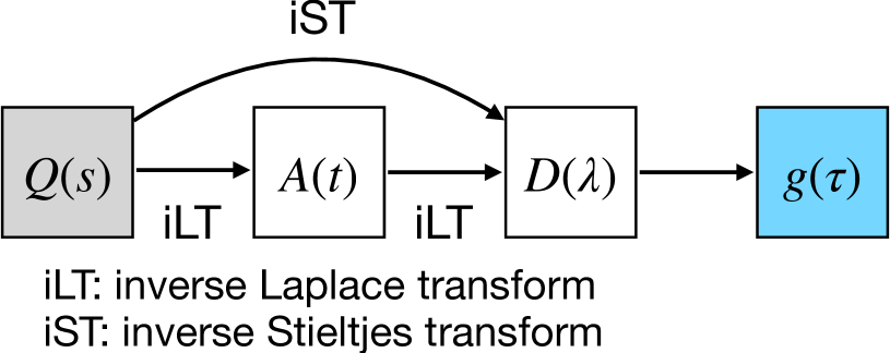
Figure 1: Basic relations between the functions $Q(s)$, $A(t)$, $D(\lambda)$ and $g(\tau)$ ($g(\tau)=\tau^{-1}D(\tau^{-1})$ with $\tau=\lambda^{-1}$)

One simple example to demonstrate these steps is to consider the case of a series $RC$ circuit with an admittance given by

$$Y(s)=\frac{sC}{1+RCs}$$ (17)

In normalized form this admittance is:

$$\frac{Y(s)}{sC}=Q_{1}(s)=\frac{1}{1+s\tau_{0}}$$ (18)

where $\tau_{0}=RC$ is a time constant. Its inverse LT gives:

$$A_{1}(t)={\tau_{0}}^{-1}e^{-t/\tau_{0}}$$ (19)

and by another iteration of inverse LT we obtain:

$$D_{1}(\lambda)=\tau_{0}^{-1}\delta(\lambda-\tau_{0}^{-1})$$ (20)

Using Eq. 16, we obtain for the DFRT:

$$g_{1}(\tau)=\tau^{-1}\tau_{0}^{-1}\delta(\tau^{-1}-\tau_{0}^{-1})=\delta(\tau-\tau_{0})$$ (21)

which is as expected an impulse delayed by $\tau_{0}$.

The procedure for deriving expressions for $g(\tau)$ can be streamlined and generalized with use of Fox’s $H$-function Fox (1961), as we show below. The use of the $H$-function is motivated by the fact that it has many convenient properties and amongst them is that its Laplace transform is again an $H$-function Mathai, Saxena, and Haubold (2009). This allows us to obtain both the system response function and the DFRT in a straightforward manner in terms of the $H$-function.

II.2 Proposed method of inversion

The procedure we propose here for deconvolving the DFRT $g(\tau)$ from Eq. 5 requires first to express a given impedance function in terms of Fox’s $H$-function. We recall that Fox’s $H$-function of order $(m,n,p,q)\in\mathbb{N}^{4}$, ($0\leqslant n\leqslant p$, $1\leqslant m\leqslant q$) and with parameters $A_{j}\in\mathbb{R}_{+}\;(j=1,\ldots,p)$, $B_{j}\in\mathbb{R}_{+}\;(j=1,\ldots,q)$, $a_{j}\in\mathbb{C}\;(j=1,\ldots,p)$ and $b_{j}\in\mathbb{C}\;(j=1,\ldots,q)$ is defined for $z\in\mathbb{C},\;z\neq 0$ by the contour integral Fox (1961); Mathai, Saxena, and Haubold (2009):

$$H^{m,n}_{p,q}\left[z|^{(a_{1},A_{1}),\ldots,(a_{p},A_{p})}_{(b_{1},B_{1}),\ldots,(b_{q},B_{q})}\right]=\frac{1}{2\pi i}\int_{L}h(s)z^{-s}ds$$ (22)

where the integrand $h(s)$ is given by:

$$h(s)=\frac{\left\{\prod\limits_{j=1}^{m}\Gamma(b_{j}+B_{j}s)\right\}\left\{\prod\limits_{j=1}^{n}\Gamma(1-a_{j}-A_{j}s)\right\}}{\left\{\prod\limits_{j={m+1}}^{q}\Gamma(1-b_{j}-B_{j}s)\right\}\left\{\prod\limits_{j={n+1}}^{p}\Gamma(a_{j}+A_{j}s)\right\}}$$ (23)

In Eq. 22, $z^{-s}=\exp\left[-s(\ln|z|+i\arg z)\right]$ and $\arg z$ is not necessarily the principal value. The contour of integration $L$ is a suitable contour separating the poles of $\Gamma(b_{j}+B_{j}s)$ ($j=1,\ldots,m$) from the poles of $\Gamma(1-a_{j}-A_{j}s)$ ($j=1,\ldots,n$). An empty product is always interpreted as unity. For more details on the $H$-function including definition, convergence, and many useful properties we refer to Mathai, Saxena, and Haubold Mathai, Saxena, and Haubold (2009), Mathai and Saxena Mathai et al. (1978), and Kilbas and Saigo Kilbas (2004).

The importance of the $H$-function for this work arises from that fact that (i) it contains a vast number of elementary and special functions used in science and engineering as special cases; see for instance Appendices A.6 and A.7 in Mathai and Saxena Mathai et al. (1978) for many examples of elementary functions expressed in terms of $H$-functions, and $H$-functions expressed in terms of elementary functions. Furthermore, (ii) the Laplace transform of an $H$-function is again an $H$-function, which is essentially the main mathematical tool needed to deal with Eq. 11. This result is obtained from the following steps Hilfer (2002); Glöckle and Nonnenmacher (1993):

$$\mathcal{L} \left[H_{p,q}^{m,n}\left[t\left|\begin{array}[]{c}(a_{p},A_{p})\\ (b_{q},B_{q})\\ \end{array}\right.\right];u\right]$$ (26)

$$=\frac{1}{2\pi i}\int_{0}^{\infty}\int_{L}e^{-ut}h(s)t^{-s}ds\,dt$$

$$=\frac{1}{2\pi i}\int_{L}h(s)u^{s-1}\Gamma(1-s)ds$$

$$=u^{-1}H^{m,n+1}_{p+1,q}\left[u^{-1}\left|\begin{array}[]{c}(0,1),(a_{1},A_{1}),\ldots,(a_{p},A_{p})\\ (b_{1},B_{1}),\ldots,(b_{q},B_{q})\\ \end{array}\right.\right]$$ (29)

Furthermore, we have the inverse LT given by Glöckle and Nonnenmacher (1993):

$$\mathcal{L}^{-1} \left[H^{m,n}_{p,q}\left[u\left|\begin{array}[]{c}(a_{p},A_{p})\\ (b_{q},B_{q})\\ \end{array}\right.\right];t\right]$$ (32)

$$=t^{-1}H^{m,n}_{p+1,q}\left[t^{-1}\left|\begin{array}[]{c}(a_{p},A_{p}),\ldots,(a_{1},A_{1}),(0,1)\\ (b_{1},B_{1}),\ldots,(b_{q},B_{q})\\ \end{array}\right.\right]$$ (35)

From Mathai, Saxena and Haubold Mathai, Saxena, and Haubold (2009) (formula 2.19), we have:

$$\mathcal{L} \left[t^{\rho-1}H_{p,q}^{m,n}\left[at^{\sigma}\left|\begin{array}[]{c}(a_{p},A_{p})\\ (b_{q},B_{q})\\ \end{array}\right.\right];u\right]$$ (38)

$$=u^{-\rho}H^{m,n+1}_{p+1,q}\left[au^{-\sigma}\left|\begin{array}[]{c}(1-\rho,\sigma),(a_{1},A_{1}),\ldots,(a_{p},A_{p})\\ (b_{1},B_{1}),\ldots,(b_{q},B_{q})\\ \end{array}\right.\right]$$ (41)

which uses extra parameters ($a,\rho,\sigma$) in case they are needed. Its inverse LT (formula 2.21 in Mathai, Saxena, and Haubold (2009)) is:

$$\mathcal{L}^{-1} \left[u^{-\rho}H_{p,q}^{m,n}\left[au^{\sigma}\left|\begin{array}[]{c}(a_{p},A_{p})\\ (b_{q},B_{q})\\ \end{array}\right.\right];t\right]$$ (44)

$$=t^{\rho-1}H_{p+1,q}^{m,n}\left[at^{-\sigma}\left|\begin{array}[]{c}(a_{p},A_{p}),\ldots,(a_{1},A_{1}),(\rho,\sigma)\\ (b_{1},B_{1}),\ldots,(b_{q},B_{q})\\ \end{array}\right.\right]$$ (47)

Now using Eqs. 11 and 16 with the help of a few general properties of the $H$-function, mainly (i) identities dealing with the reciprocal of an argument Kilbas (2004); Mathai et al. (1978); Mathai, Saxena, and Haubold (2009):

$$H^{m,n}_{p,q}\left[z\left|\begin{array}[]{l}(a_{p},A_{p})\\ (b_{q},B_{q})\\ \end{array}\right.\right]=H^{n,m}_{q,p}\left[z^{-1}\left|\begin{array}[]{l}(1-b_{q},B_{q})\\ (1-a_{p},A_{p})\\ \end{array}\right.\right],$$ (48)

and (ii) the multiplication of an $H$-function by the argument to a certain power:

$$z^{\sigma}H^{m,n}_{p,q}\left[z\left|\begin{array}[]{l}(a_{p},A_{p})\\ (b_{q},B_{q})\\ \end{array}\right.\right]=H^{m,n}_{p,q}\left[z\left|\begin{array}[]{l}(a_{p}+\sigma A_{p},A_{p})\\ (b_{q}+\sigma B_{q},B_{q})\\ \end{array}\right.\right]$$ (49)

leads to the desired result for the DFRT $g(\tau)$. In Section III below we apply this procedure to a few examples of well-known impedance functions.

III Examples

III.1 Constant phase element

The constant phase element (CPE) is widely used in equivalent circuit models for impedance fitting of anomalous data that cannot be easily described with basic $R$ and $C$ circuit elements Allagui et al. (2016); Lasia (2022); Gateman et al. (2022); Allagui et al. (2020); Allagui and Fouda (2021). Its impedance function is given by:

$$Z_{c}(s)=\frac{1}{C_{\alpha}s^{\alpha}}$$ (50)

where $C_{\alpha}$ is a pseudo-capacitance in units of F s^α-1 and $\alpha$ is known as the dispersion coefficient. For $0<\alpha\leqslant 1$, the CPE represents the impedance of a fractional capacitor of constant phase $\phi(Z_{c})=\tan^{-1}(-\alpha\pi/2)$, and for $\alpha=1$, it represents the impedance of an ideal capacitor. For the particular case of $\alpha=0.5$, it represents the Warburg impedance. Normalizing the impedance function in Eq. 50 to an arbitrary resistance $R$ gives:

$$Q_{c}(s)=\frac{1}{(s\tau_{c})^{\alpha}}$$ (51)

where $\tau_{c}=(RC_{\alpha})^{1/\alpha}$ is a characteristic time constant. Applying two successive times the inverse LT to $Q_{c}(s)$ gives first the system response function as:

$$A_{c}(t)=\frac{(t/\tau_{c})^{\alpha}}{t\,\Gamma(\alpha)}$$ (52)

and then the distribution $D_{c}(\lambda)$ as:

$$D_{c}(\lambda)=\pi^{-1}\sin(\alpha\pi)(\tau_{c}\,\lambda)^{-\alpha}$$ (53)

We remind that ${\pi}/{\sin(\pi z)}=\Gamma(z)\Gamma(1-z)$ (reflection formula for the gamma function). Using Eq. 16 we obtain the DFRT $g_{c}(\tau)$ as the power-law function Barsoukov and Macdonald (2018):

$$g_{c}(\tau)=\pi^{-1}\sin(\alpha\pi)\tau_{c}^{-\alpha}\tau^{\alpha-1}$$ (54)

We note that $D_{c}(\lambda)$ can be obtained directly through the inverse ST applied onto Eq. 51 using Bateman (1954):

$$s^{-\alpha}=\frac{1}{\Gamma(\alpha)\Gamma(1-\alpha)}\int\limits_{0}^{\infty}\frac{\lambda^{-\alpha}}{s+\lambda}d\lambda$$ (55)

or thought the Titchmarsh inversion formula (# 11.8.4 in Titchmarsh (1948)):

$$D_{c}(\lambda)=\frac{i}{2\pi}\left[Q_{c}(\lambda e^{i\pi})-Q_{c}(\lambda e^{-i\pi})\right]$$ (56)

Discretization of Eq. 55 has been adapted by Abdelaty et al. AbdelAty et al. (2018) as a way of representing the $s^{\alpha}$ term as a weighted sum of first-order high-pass filters.

Now in order to apply the proposed inversion method, we rewrite the CPE impedance function in Eq. 51 as an $H$-function using the following relation Mathai, Saxena, and Haubold (2009):

$${z^{\gamma}}(1-z)^{\beta}=\Gamma(\beta+1)H^{1,0}_{1,1}\left[z\left|\begin{array}[]{c}(\gamma+\beta+1,1)\\ (\gamma,1)\hfill\\ \end{array}\right.\right]$$ (59)

which gives:

$$Q_{c}(s)=H^{1,0}_{1,1}\left[(s\tau_{c})\left|\begin{array}[]{c}(-\alpha+1,1)\\ (-\alpha,1)\hfill\\ \end{array}\right.\right]$$ (62)

valid for the argument $|s\tau_{c}|<1$, and

$$Q_{c}(s)=H^{0,1}_{1,1}\left[(s\tau_{c})\left|\begin{array}[]{c}(-\alpha+1,1)\\ (-\alpha,1)\hfill\\ \end{array}\right.\right]$$ (65)

valid for $|s\tau_{c}|>1$. We note that when $A_{i}=B_{j}=1$ $(i=1,\ldots,p)$; $(j=1,\ldots,q)$ the $H$-function reduces to the Meijer $G$-function Kilbas (2004). This makes Eq. 65 for instance to be:

$$Q_{c}(s)=G^{0,1}_{1,1}\left[(s\tau_{c})\left|\begin{array}[]{c}(-\alpha+1)\\ (-\alpha)\hfill\\ \end{array}\right.\right]$$ (68)

The inverse LT of Eq. 65 using the formula given in 44 (with the help of the identity 48) is:

$$A_{c}(t) =t^{-1}H^{0,1}_{2,1}\left[(\tau_{c}/t)\left|\begin{array}[]{c}(-\alpha+1,1),(0,1)\\ (-\alpha,1)\hfill\\ \end{array}\right.\right]$$ (71)

$$=t^{-1}H^{1,0}_{1,2}\left[(t/\tau_{c})\left|\begin{array}[]{c}(1+\alpha,1)\hfill\\ (\alpha,1),(1,1)\\ \end{array}\right.\right]$$ (74)

$$=\frac{(t/\tau_{c})^{\alpha}}{t\,\Gamma(\alpha)}$$ (75)

from which:

$$D_{c}(\lambda)=H^{1,0}_{2,2}\left[(\lambda\,\tau_{c})^{-1}\left|\begin{array}[]{c}(1+\alpha,1),(1,1)\\ (\alpha,1),(1,1)\hfill\\ \end{array}\right.\right]$$ (78)

Then using Eq. 16, we obtain the DFRT for a CPE impedance as:

$$g_{c}(\tau)=\tau^{-1}H^{1,0}_{2,2}\left[(\tau/\tau_{c})\left|\begin{array}[]{c}(1+\alpha,1),(1,1)\\ (\alpha,1),(1,1)\hfill\\ \end{array}\right.\right]$$ (81)

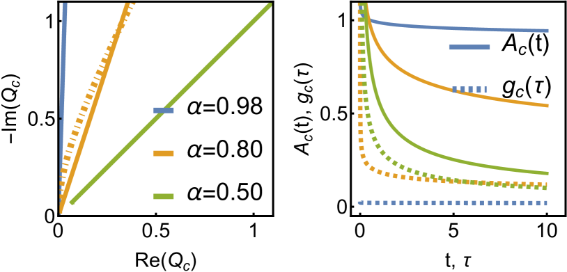
Figure 2: Plots of (a) $Q_{c}(s)$ (Eqs. 62 and 65) in Nyquist form of real vs. imaginary parts for $\tau_{c}=1$ and $\alpha=$ 0.98, 0.80 and 0.50. In dot-dashed we plot the discretized version of Eq. 9 with $g(\tau)=g_{c}(\tau)$ for values of $\tau$ varying from 0.5 to 1000 s at a step of 0.1 s. In (b) we plot the functions $A_{c}(t)$ and $g_{c}(\tau)$ for the same parameters: $\tau_{c}=1$ and $\alpha=$ 0.98, 0.80 and 0.50

In Fig. 2 we show plots of the three functions $Q_{c}(s)$, $A_{c}(t)$ and $g_{c}(\tau)$ for the case of $\tau_{c}=1$ and for the three values of $\alpha=0.98,0.80,0.50$ . The frequency range for the Nyquist plot of $Q_{c}(s)$ is 0.01 to 100 Hz. One can clearly see the gradual deviation of the plots from the ideal case of a capacitor ($\alpha=1$) as the value of $\alpha$ is reduced. We also plotted in Fig. 2(a), in dot-dashed line, the discretized version of Eq. 9 with $g(\tau)=g_{c}(\tau)$ for $\alpha=0.80$ and for values of $\tau$ varying from 0.5 to 1000 s at a step of 0.1 s.

III.2 Davidson-Cole Model

The Davidson-Cole model is given by Davidson and Cole (1951):

$$Q_{\gamma}(s)=\frac{1}{(1+s\tau_{\gamma})^{\gamma}}\quad(0<\gamma\leqslant 1)$$ (82)

Using the formula Mathai, Saxena, and Haubold (2009):

$$(1-z)^{-\alpha}=\frac{1}{\Gamma(\alpha)}H^{1,1}_{1,1}\left[-z\left|\begin{array}[]{c}(1-\alpha,1)\\ (0,1)\hfill\\ \end{array}\right.\right]$$ (85)

we rewrite $Q_{\gamma}(s)$ as:

$$Q_{\gamma}(s)=\frac{1}{\Gamma(\gamma)}H^{1,1}_{1,1}\left[s\tau_{\gamma}\left|\begin{array}[]{c}(1-\gamma,1)\\ (0,1)\hfill\\ \end{array}\right.\right]$$ (88)

The inverse LT of Eq. 82 is:

$$A_{\gamma}(t)=\frac{\left({t}/{\tau_{\gamma}}\right)^{\gamma}e^{-{t}/{\tau_{\gamma}}}}{t\,\Gamma(\gamma)}$$ (89)

which can be represented in terms of the $H$-function as:

$$A_{\gamma}(t)=\frac{1}{{\tau_{\gamma}\,\Gamma(\gamma)}}H_{0,1}^{1,0}\left[t/\tau_{\gamma}\left|\begin{array}[]{c}-\\ (\gamma-1,1)\hfill\\ \end{array}\right.\right]$$ (90)

Using the inverse LT formula 44 on Eq. 88 gives:

$$A_{\gamma}(t) =\frac{1}{t\,\Gamma(\gamma)}H^{1,1}_{1,2}\left[t/\tau_{\gamma}\left|\begin{array}[]{c}(1,1)\hfill\\ (\gamma,1),(1,1)\\ \end{array}\right.\right]$$ (93)

$$=\frac{1}{\tau_{\gamma}\Gamma(\gamma)}H^{1,1}_{1,2}\left[t/\tau_{\gamma}\left|\begin{array}[]{c}(0,1)\hfill\\ (\gamma-1,1),(0,1)\\ \end{array}\right.\right]$$ (96)

The latter can be readily reduced to Eq. 90 using Mathai, Saxena, and Haubold (2009):

$$H^{m,n}_{p,q} \left[z\left|\begin{array}[]{l}(a_{1},A_{1}),\ldots,(a_{p},A_{p})\\ (b_{1},B_{1}),\ldots,(b_{q-1},B_{q-1}),(a_{1},A_{1})\\ \end{array}\right.\right]$$ (99)

$$= H^{m,n-1}_{p-1,q-1}\left[z\left|\begin{array}[]{l}(a_{2},A_{2}),\ldots,(a_{p},A_{p})\\ (b_{1},B_{1}),\ldots,(b_{q-1},B_{q-1})\\ \end{array}\right.\right]$$ (102)

This formula is applicable if one of $(a_{j},A_{j})\;(j=1,\ldots,n)$ is equal to one of the $(b_{j},B_{j})\;(j=m+1,\ldots,q)$ or one of the $(b_{j},B_{j})\;(j=1,\ldots,m)$ is equal to one of the $(a_{j},A_{j})\;(j=n+1,\ldots,p)$, provided that $n\geqslant 1$ and $q\geqslant m$.

By another round of inverse LT applied on $A_{\gamma}(t)$ given in Eq. 89 we obtain:

$$D_{\gamma}(\lambda)=\frac{\sin(\gamma\pi)}{\pi}\theta\left(\lambda-{\tau_{\gamma}^{-1}}\right)(\lambda\tau_{\gamma}-1)^{-\gamma}$$ (103)

and Barsoukov and Macdonald (2018)

$$g_{\gamma}(\tau)=\frac{\sin(\gamma\pi)}{\pi}\theta\left(\tau^{-1}-{\tau_{\gamma}^{-1}}\right)\tau^{-1}(\tau_{\gamma}/\tau-1)^{-\gamma}$$ (104)

i.e.:

$$g_{\gamma}(\tau) =\frac{\sin(\gamma\pi)}{\pi}\tau^{-1}(\tau_{\gamma}/\tau-1)^{-\gamma},\;\;\tau<\tau_{\gamma}$$

$$=0,\;\;\text{otherwise}$$ (105)

Similarly, we obtain from the $H$-function representation of $A_{\gamma}(t)$ (i.e. Eq. 96):

$$D_{\gamma}(\lambda) =\frac{(\tau_{\gamma}\lambda)^{-1}}{\Gamma(\gamma)}H^{1,1}_{2,2}\left[(\tau_{\gamma}\lambda)^{-1}\left|\begin{array}[]{l}(0,1),(0,1)\\ (\gamma-1,1),(0,1)\\ \end{array}\right.\right]$$ (108)

$$=\frac{1}{\Gamma(\gamma)}H^{1,1}_{2,2}\left[(\tau_{\gamma}\lambda)^{-1}\left|\begin{array}[]{l}(1,1),(1,1)\\ (\gamma,1),(1,1)\\ \end{array}\right.\right]$$ (111)

and

$$g_{\gamma}(\tau)=\frac{1}{\tau_{\gamma}\,\Gamma(\gamma)}H^{1,0}_{1,1}\left[\tau/\tau_{\gamma}\left|\begin{array}[]{c}(0,1)\hfill\\ (\gamma-1,1)\\ \end{array}\right.\right]$$ (114)

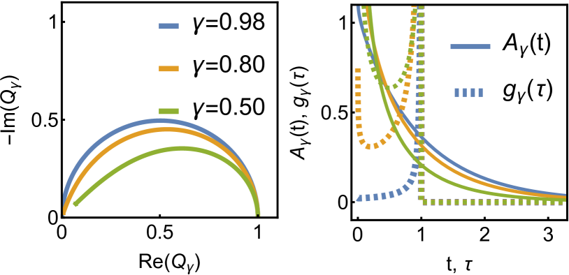
Figure 3: Plots of (a) $Q_{\gamma}(s)$ (Eq. 88) in Nyquist form of real vs. imaginary parts for $\tau_{c}=1$ and $\gamma=$ 0.98, 0.80 and 0.50. In (b) we plot the functions $A_{\gamma}(t)$ (Eq. 93) and $g_{\gamma}(\tau)$ (Eq. 114) for the same parameters: $\tau_{\gamma}=1$ and $\gamma=$ 0.98, 0.80 and 0.50

For illustration, we show in Fig. 3 plots of $Q_{\gamma}(s)$ (Eq. 88), $A_{\gamma}(t)$ (Eq. 93) and $g_{\gamma}(\tau)$ (Eq. 114) for $\tau_{\gamma}=1$ and $\gamma=$ 0.98, 0.80 and 0.50. We see clearly the cutoff of $g_{\gamma}(\tau)$ for values of $\tau>\tau_{\gamma}$.

III.3 Cole-Cole model

The Cole-Cole model is given by Cole and Cole (1941):

$$Q_{\alpha}(s)=\frac{1}{1+(s\tau_{\alpha})^{\alpha}}\quad(0<\alpha\leqslant 1)$$ (115)

in its traditional form, which can be rewritten in terms of the $H$-function as:

$$Q_{\alpha}(s)=H^{1,1}_{1,1}\left[(s\tau_{\alpha})^{\alpha}\left|\begin{array}[]{c}(0,1)\\ (0,1)\\ \end{array}\right.\right]$$ (118)

This is obtained from Mathai, Saxena, and Haubold (2009):

$$\frac{z^{\beta}}{1+az^{\alpha}}=a^{\beta/\alpha}H^{1,1}_{1,1}\left[az^{\alpha}\left|\begin{array}[]{c}(\beta/\alpha,1)\\ (\beta/\alpha,1)\\ \end{array}\right.\right]$$ (121)

The inverse LT of Eq. 115 from the Prabhakar integral Prabhakar (1971); Saxena, Mathai, and Haubold (2004):

$$\int\limits_{0}^{\infty}t^{\beta-1}{E}_{\alpha,\beta}^{\gamma}\left(-at^{\alpha}\right)e^{-st}dt=\frac{s^{-\beta}}{(1+as^{-\alpha})^{\gamma}}$$ (122)

with $\alpha=\beta$, $\gamma=1$ and $a=\tau_{\alpha}^{-\alpha}$ gives the system response function $A_{\alpha}(t)$ as:

$$A_{\alpha}(t)=\tau_{\alpha}^{-1}({t}/{\tau_{\alpha}})^{\alpha-1}E_{\alpha,\alpha}^{1}\left[-(t/\tau_{\alpha})^{\alpha}\right]$$ (123)

The function

$${E}_{\alpha,\beta}^{\gamma}(z):=\sum\limits_{k=0}^{\infty}\frac{(\gamma)_{k}}{\Gamma(\alpha k+\beta)}\frac{z^{k}}{k!}\quad(\alpha,\beta,\gamma\in\mathbb{C},\mathrm{Re}({\alpha})>0)$$ (124)

with $(\gamma)_{k}=\gamma(\gamma+1)\ldots(\gamma+k-1)=\Gamma(\gamma+k)/\Gamma(\gamma)$ being the Pochhammer symbol is the three-parameter Mittag-Leffler function. Eq. 123 can be expressed in terms of Fox’s $H$-function as:

$$A_{\alpha}(t)=\tau_{\alpha}^{-1}({t}/{\tau_{\alpha}})^{\alpha-1}H^{1,1}_{1,2}\left[(t/\tau_{\alpha})^{\alpha}\left|\begin{array}[]{l}{(0,1)\hfill}\\ {(0,1),(1-\alpha,\alpha)}\end{array}\right.\right]$$ (125)

Using the property 49, with $\sigma=1-1/\alpha$, Eq. 125 turns to be:

$$A_{\alpha}(t)=\tau_{\alpha}^{-1}H^{1,1}_{1,2}\left[(t/\tau_{\alpha})^{\alpha}\left|\begin{array}[]{l}{(1-1/\alpha,1)}\\ {(1-1/\alpha,1),(0,\alpha)}\\ \end{array}\right.\right]$$ (126)

Now we apply the inverse LT formula given in 44 on $Q(s)$ given by Eq 118. This leads to:

$$A_{\alpha}(t) =\mathcal{L}^{-1}\left[H_{1,1}^{1,1}\left[(s\tau_{\alpha})^{\alpha}\left|\begin{array}[]{c}(0,1)\\ (0,1)\\ \end{array}\right.\right];t\right]$$ (129)

$$=t^{-1}H^{1,1}_{2,1}\left[(t/\tau_{\alpha})^{-\alpha}\left|\begin{array}[]{c}(0,1),(0,\alpha)\\ (0,1)\hfill\\ \end{array}\right.\right]$$ (132)

With the use of the property 48, $A_{\alpha}(t)$ in Eq 132 becomes:

$$A_{\alpha}(t)=t^{-1}H^{1,1}_{1,2}\left[(t/\tau_{\alpha})^{\alpha}\left|\begin{array}[]{l}{(1,1)}\\ {(1,1),(1,\alpha)}\\ \end{array}\right.\right]$$ (133)

and then, with the property 49 with $\sigma=-1/\alpha$, we obtain the same result as given in Eq 126.

From $A_{\alpha}(t)$ we can now derive $D_{\alpha}(\lambda)$ by another iteration of inverse LT. This gives (after using property 49):

$$D_{\alpha}(\lambda) =\mathcal{L}^{-1}\left[\tau_{\alpha}^{-1}H^{1,1}_{1,2}\left[(t/\tau_{\alpha})^{\alpha}|^{(1-1/\alpha,1)}_{(1-1/\alpha,1),(0,\alpha)}\right];\lambda\right]$$

$$=H^{1,1}_{2,2}\left[(\tau_{\alpha}\lambda)^{-\alpha}\left|\begin{array}[]{c}(1,1),(1,\alpha)\\ (1,1),(1,\alpha)\\ \end{array}\right.\right]$$ (136)

With Eq. 16 and then formula 49, we obtain for the DFRT $g(\tau)$:

$$g_{\alpha}(\tau)=\tau_{\alpha}^{-1}H^{1,1}_{2,2}\left[(\tau/\tau_{\alpha})^{\alpha}\left|\begin{array}[]{c}(1-1/\alpha,1),(0,\alpha)\\ (1-1/\alpha,1),(0,\alpha)\\ \end{array}\right.\right]$$ (137)

III.4 Havriliak–Negami model

Combining both the Cole-Cole and Davidson–Cole models results in the Havriliak–Negami model Havriliak and Negami (1966):

$$Q_{\nu}(s) =\frac{1}{(1+(s\tau_{{\nu}})^{\alpha})^{\gamma}}\quad(0<\alpha,\gamma\leqslant 1)$$ (138)

$$=\frac{1}{\Gamma(\gamma)}H^{1,1}_{1,1}\left[(s\tau_{\nu})^{\alpha}\left|\begin{array}[]{c}(1-\gamma,1)\\ (0,1)\hfill\\ \end{array}\right.\right]$$ (141)

It is easy to verify that for the special case of $\gamma=1$, Eq. 141 reduces to the Cole-Cole relation (Eq. 118), and in the case that $\alpha=1$, the Davidson-Cole relation is obtained (Eq. 88). By operating a first LT inversion on $Q_{\nu}(s)$ (using Eq. 122 and Eq. 44) we obtain:

$$A_{\nu}(t) =\tau_{\nu}^{-1}({t}/{\tau_{\nu}})^{\alpha\gamma-1}E_{\alpha,\alpha\gamma}^{\gamma}\left[-(t/\tau_{\nu})^{\alpha}\right]$$ (142)

$$=\frac{1}{t\,\Gamma(\gamma)}H^{1,1}_{1,2}\left[(t/\tau_{\nu})^{\alpha}\left|\begin{array}[]{c}(1,1)\hfill\\ (\gamma,1),(1,\alpha)\\ \end{array}\right.\right]$$ (145)

and then again on $A_{\nu}(t)$ with the use of Eq. 16 leads to:

$$g_{\nu}(\tau)=\frac{1}{\tau_{\nu}\Gamma(\gamma)}H^{1,1}_{2,2}\left[(\tau/\tau_{\nu})^{\alpha}\left|\begin{array}[]{c}(1-1/\alpha,1),(0,\alpha)\\ (\gamma-1/\alpha,1),(0,\alpha)\\ \end{array}\right.\right]$$ (146)

We verify that the response function in Eq. 145 reduces to that given by Eq. 133 for $\gamma=1$ (Cole-Cole model), and to Eq. 93 for $\alpha=1$ (Davidson-Cole model). The DFRT in Eq. 146 reduces to Eq. 137 for $\gamma=1$, and to Eq. 114 for $\alpha=1$.

Plots of $Q_{\nu}(s)$ (Eq. 141), $A_{\nu}(t)$ (Eq. 145), and $g_{\tau}(s)$ (Eq. 146) for $\tau_{\nu}=1$ and a combination of values of $\alpha$ and $\gamma$ (Cole-Cole model for $\gamma=1$) are given in Fig. 4.

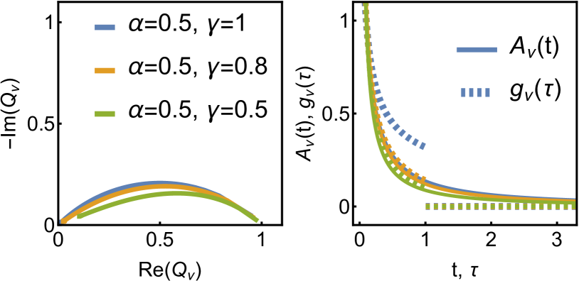
Figure 4: Plots of (a) $Q_{\nu}(s)$ (Eq. 141) in Nyquist form of real vs. imaginary parts for $\tau_{\nu}=1$, $\alpha=0.5$ and $\gamma=$ 1, 0.80 and 0.50. In (b) we plot the functions $A_{\nu}(t)$ (Eq. 145) and $g_{\nu}(\tau)$ (Eq. 146) for the same parameters $\tau_{\nu}$, $\alpha$ and $\gamma$

IV Conclusion

With the assumption that a system can be represented by an infinite number of $RC$ branches, the distribution function of the $RC$ time constants is related to the impedance model via two iterated Laplace transforms. We showed in this paper a general procedure for how to deconvolve the DFRT starting from any arbitrary impedance model represented in terms of the Fox $H$-function.

References

References

- Barsoukov and Macdonald (2018) E. Barsoukov and J. R. Macdonald, Impedance spectroscopy: theory, experiment, and applications (John Wiley & Sons, 2018).
- Lasia (2014) A. Lasia, Electrochemical impedance spectroscopy and its applications (Springer, 2014).
- Single, Horstmann, and Latz (2019) F. Single, B. Horstmann, and A. Latz, “Theory of impedance spectroscopy for lithium batteries,” J. Phys. Chem. C 123, 27327–27343 (2019).
- Bredar et al. (2020) A. R. Bredar, A. L. Chown, A. R. Burton, and B. H. Farnum, “Electrochemical impedance spectroscopy of metal oxide electrodes for energy applications,” ACS Appl. Energy Mater. 3, 66–98 (2020).
- Vadhva et al. (2021) P. Vadhva, J. Hu, M. J. Johnson, R. Stocker, M. Braglia, D. J. Brett, and A. J. Rettie, “Electrochemical impedance spectroscopy for all-solid-state batteries: Theory, methods and future outlook,” ChemElectroChem 8, 1930–1947 (2021).
- Allagui et al. (2016) A. Allagui, A. S. Elwakil, B. J. Maundy, and T. J. Freeborn, “Spectral capacitance of series and parallel combinations of supercapacitors,” ChemElectroChem 3, 1429–1436 (2016).
- He and Mansfeld (2009) Z. He and F. Mansfeld, “Exploring the use of electrochemical impedance spectroscopy (eis) in microbial fuel cell studies,” Energy Environ. Sci. 2, 215–219 (2009).
- Guerrero, Bisquert, and Garcia-Belmonte (2021) A. Guerrero, J. Bisquert, and G. Garcia-Belmonte, “Impedance spectroscopy of metal halide perovskite solar cells from the perspective of equivalent circuits,” Chem. Rev. 121, 14430–14484 (2021).
- Pejcic and De Marco (2006) B. Pejcic and R. De Marco, “Impedance spectroscopy: Over 35 years of electrochemical sensor optimization,” Electrochim. Acta 51, 6217–6229 (2006).
- Mansfeld (1990) F. Mansfeld, “Electrochemical impedance spectroscopy (eis) as a new tool for investigating methods of corrosion protection,” Electrochim. Acta 35, 1533–1544 (1990).
- Cesewski and Johnson (2020) E. Cesewski and B. N. Johnson, “Electrochemical biosensors for pathogen detection,” Biosens. Bioelectron. 159, 112214 (2020).
- Lisdat and Schäfer (2008) F. Lisdat and D. Schäfer, “The use of electrochemical impedance spectroscopy for biosensing,” Anal. Bioanal.Chem. 391, 1555–1567 (2008).
- Effendy, Song, and Bazant (2020) S. Effendy, J. Song, and M. Z. Bazant, “Analysis, design, and generalization of electrochemical impedance spectroscopy (eis) inversion algorithms,” J. Electrochem. Soc. 167, 106508 (2020).
- Ciucci and Chen (2015) F. Ciucci and C. Chen, “Analysis of electrochemical impedance spectroscopy data using the distribution of relaxation times: A bayesian and hierarchical bayesian approach,” Electrochim. Acta 167, 439–454 (2015).
- Allagui and Fouda (2021) A. Allagui and M. E. Fouda, “Inverse problem of reconstructing the capacitance of electric double-layer capacitors,” Electrochim. Acta , 138848 (2021).
- Allagui, Elwakil, and Fouda (2021) A. Allagui, A. S. Elwakil, and M. E. Fouda, “Revisiting the time-domain and frequency-domain definitions of capacitance,” IEEE Trans. Electron Devices 68 (2021).
- Florsch, Revil, and Camerlynck (2014) N. Florsch, A. Revil, and C. Camerlynck, “Inversion of generalized relaxation time distributions with optimized damping parameter,” J. Appl. Geophys. 109, 119–132 (2014).
- Schichlein et al. (2002) H. Schichlein, A. C. Müller, M. Voigts, A. Krügel, and E. Ivers-Tiffée, “Deconvolution of electrochemical impedance spectra for the identification of electrode reaction mechanisms in solid oxide fuel cells,” J. Appl. Electrochem. 32, 875–882 (2002).
- Boukamp (2015) B. A. Boukamp, “Fourier transform distribution function of relaxation times; application and limitations,” Electrochimica acta 154, 35–46 (2015).
- Gavrilyuk, Osinkin, and Bronin (2017) A. Gavrilyuk, D. Osinkin, and D. Bronin, “The use of tikhonov regularization method for calculating the distribution function of relaxation times in impedance spectroscopy,” Russ. J. Electrochem. 53, 575–588 (2017).
- Paul et al. (2021) T. Paul, P. Chi, P. M. Wu, and M. Wu, “Computation of distribution of relaxation times by tikhonov regularization for li ion batteries: usage of l-curve method,” Sci. Rep. 11, 12624 (2021).
- Shanbhag (2020) S. Shanbhag, “Relaxation spectra using nonlinear tikhonov regularization with a bayesian criterion,” Rheol. Acta 59, 509–520 (2020).
- Hörlin (1998) T. Hörlin, “Deconvolution and maximum entropy in impedance spectroscopy of noninductive systems,” Solid State Ionics 107, 241–253 (1998).
- Hörlin (1993) T. Hörlin, “Maximum entropy in impedance spectroscopy of non-inductive systems,” Solid State Ionics 67, 85–96 (1993).
- Tesler et al. (2010) A. Tesler, D. Lewin, S. Baltianski, and Y. Tsur, “Analyzing results of impedance spectroscopy using novel evolutionary programming techniques,” J. Electroceram. 24, 245–260 (2010).
- Boukamp (2020) B. A. Boukamp, “Distribution (function) of relaxation times, successor to complex nonlinear least squares analysis of electrochemical impedance spectroscopy?” J. Phys.: Energy 2, 042001 (2020).
- Liu and Ciucci (2020) J. Liu and F. Ciucci, “The deep-prior distribution of relaxation times,” J. Electrochem. Soc. 167, 026506 (2020).
- Macdonald and Brachman (1956) J. R. Macdonald and M. K. Brachman, “Linear-system integral transform relations,” Reviews of modern physics 28, 393 (1956).
- Bateman (1954) H. Bateman, Tables of integral transforms, Vol. 2 (McGraw-Hill book company, 1954).
- Fox (1961) C. Fox, “The g and h functions as symmetrical fourier kernels,” Trans. Am. Math. Soc. 98, 395–429 (1961).
- Mathai, Saxena, and Haubold (2009) A. M. Mathai, R. K. Saxena, and H. J. Haubold, The H-function: theory and applications (Springer Science & Business Media, 2009).
- Mathai et al. (1978) A. M. Mathai, R. K. Saxena, R. K. Saxena, et al., The H-function with applications in statistics and other disciplines (John Wiley & Sons, 1978).
- Kilbas (2004) A. A. Kilbas, H-transforms: Theory and Applications (CRC press, 2004).
- Hilfer (2002) R. Hilfer, “-function representations for stretched exponential relaxation and non-debye susceptibilities in glassy systems,” Phys. Rev. E 65, 061510 (2002).
- Glöckle and Nonnenmacher (1993) W. G. Glöckle and T. F. Nonnenmacher, “Fox function representation of non-debye relaxation processes,” J. Stat. Phys. 71, 741–757 (1993).
- Lasia (2022) A. Lasia, “The origin of the constant phase element,” J. Phys. Chem. Lett. 13, 580–589 (2022).
- Gateman et al. (2022) S. M. Gateman, O. Gharbi, H. G. de Melo, K. Ngo, M. Turmine, and V. Vivier, “On the use of a constant phase element (cpe) in electrochemistry,” Curr. Opin. Electrochem. 36, 101133 (2022).
- Allagui et al. (2020) A. Allagui, H. Alnaqbi, A. S. Elwakil, Z. Said, A. Hachicha, C. Wang, and M. A. Abdelkareem, “Fractional-order electric double-layer capacitors with tunable low-frequency impedance phase angle and energy storage capabilities,” Appl. Phys. Lett. 116, 013902 (2020).
- Titchmarsh (1948) E. C. Titchmarsh, “Introduction to the theory of fourier integrals,” (1948).
- AbdelAty et al. (2018) A. M. AbdelAty, A. S. Elwakil, A. G. Radwan, C. Psychalinos, and B. Maundy, “Approximation of the fractional-order laplacian as a weighted sum of first-order high-pass filters,” IEEE Trans. Circuits Syst. II Express Briefs 65, 1114–1118 (2018).
- Davidson and Cole (1951) D. W. Davidson and R. H. Cole, “Dielectric relaxation in glycerol, propylene glycol, and n-propanol,” J. Chem. Phys. 19, 1484–1490 (1951).
- Cole and Cole (1941) K. S. Cole and R. H. Cole, “Dispersion and absorption in dielectrics i. alternating current characteristics,” J. Chem. Phys. 9, 341–351 (1941).
- Prabhakar (1971) T. R. Prabhakar, “A singular integral equation with a generalized mittag leffler function in the kernel,” Yokohama Math. J. 19, 7–15 (1971).
- Saxena, Mathai, and Haubold (2004) R. Saxena, A. Mathai, and H. Haubold, “On generalized fractional kinetic equations,” Physica A 344, 657–664 (2004).
- Havriliak and Negami (1966) S. Havriliak and S. Negami, “A complex plane analysis of -dispersions in some polymer systems,” in J. Polym. Sci., Part C: Polym. Symp., Vol. 14 (Wiley Online Library, 1966) pp. 99–117.