Design and Nonlinear Modeling of a Modular Cable Driven
Soft Robotic Arm
Abstract
We propose a novel multi-section cable-driven soft robotic arm inspired by octopus tentacles along with a new modeling approach. Each section of the modular manipulator is made of a soft tubing backbone, a soft silicon arm body, and two rigid endcaps, which connect adjacent sections and decouple the actuation cables of different sections. The soft robotic arm is made with casting after the rigid endcaps are 3D-printed, achieving low-cost and convenient fabrication. To capture the nonlinear effect of cables pushing into the soft silicon arm body, which results from the absence of intermediate rigid cable guides for higher compliance, an analytical static model is developed to capture the relationship between the bending curvature and the cable lengths. The proposed model shows superior prediction performance in experiments over that of a baseline model, especially under large bending conditions. Based on the nonlinear static model, a kinematic model of a multi-section arm is further developed and used to derive a motion planning algorithm. Experiments show that the proposed soft arm has high flexibility and a large workspace, and the tracking errors under the algorithm based on the proposed modeling approach are up to 52 smaller than those with the algorithm derived from the baseline model. The presented modeling approach is expected to be applicable to a broad range of soft cable-driven actuators and manipulators.
Index Terms:
soft robotics, soft manipulators, cable-driven, kinematics modeling, statics modelingI Introduction
Soft robotic manipulators have been widely proposed and developed for their various advantages, such as safe human-machine interactions, robustness, and flexibility.[1, 2, 3, 4, 5] Compared with their fully rigid counterparts, soft manipulators are able to utilize the compliance and softness of their body structures to adapt to external collisions and constraints and mitigate potential risks to humans, while being able to accomplish traditional manipulation tasks.[6, 7, 8] The advantages of soft manipulators make them competitive candidates for applications involving the handling of delicate and complex objects, as in fruit harvesting and medical surgeries.[9, 10, 11]
Multiple structures and actuation methods have been developed for building soft robotics arms to achieve compliant and efficient deformation. For example, fluid-driven methods are widely used for soft actuators, where fluid pressures inside actuator chambers are modulated to generate elastic deformation.[12, 13, 14] Soft actuators have also been constructed with other actuation mechanisms including smart materials such as electroactive polymers.[15, 16, 17, 18, 19] In particular, the cable-driven actuation method is popular thanks to its simplicity and high force-to-weight ratio,[20, 21, 22] where embedded eccentric cables driven by motors deliver torques to achieve deformation of the soft body.
To control the deformation of the soft arm effectively, models that capture the relationship between the actuation space input and the task space output of the robotic arm have been developed. This modeling process is generally complex and often dependent on robot designs and actuation methods. Models for fluid-driven actuators are often built based on static and dynamic analyses.[23, 24] For simple cable-driven actuators, models have been built based on geometry relationships.[25] Static models for tendon-driven flexible manipulators have also been proposed to analyze the deformation of the elastic tendons.[26, 27] In addition, models have been reported for the coupling and decoupling cable system of multi-section soft manipulators.[25, 28] Piecewise constant curvature (PCC) models are widely utilized due to their simplicity,[25] while other models, such as finite element method (FEM) models and Cosserat rod models are proposed with better accuracy but higher complexity.[29, 30, 31, 32] In addition, piecewise constant strain (PCS) and geometric variable strain models have been proposed that allow the incorporation of external forces and more general settings.[33, 34, 35, 36]
Many biological structures and mechanisms have inspired the design of robotic systems, and conversely, the development of robotic platforms has provided bio-physical models for understanding biology and biomechanics.[37, 38, 39, 40] In this study, inspired by the longitudinal muscles in the anatomy of octopus tentacles, we propose a decoupled modular cable-driven soft robotic arm fabricated with 3D printing and casting. We further develop a novel analytical static model that considers the prominent nonlinear effect of the cable pushing into the soft body of the robotic arm. To our best knowledge, this is the first effort in explicitly modeling the transverse deformation effect in soft cable-driven actuators, which extensively exists and might significantly influence the actuation length of the cable.
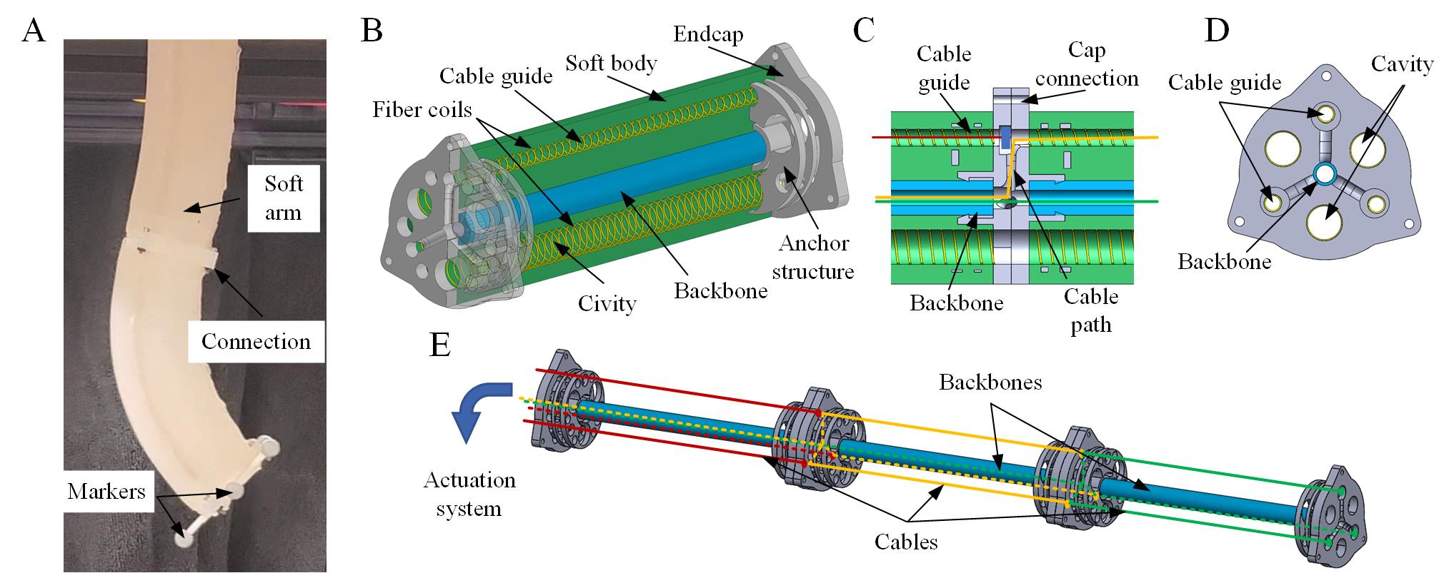
Specifically, the structure of a single section of the proposed robotic arm consists of three parts: a flexible backbone, a soft silicone body, and two rigid caps (Fig. 1B). A piece of soft tubing is selected as the backbone for its high bending flexibility and low stretchability to constrain the section length. Two rigid endcaps are attached to the ends of the backbone, which act as connectors between sections and anchor points for cables. The anchor structure is designed to achieve a robust connection between the endcaps and the soft body. The soft silicone body is made by casting with three evenly embedded fiber-reinforced cable guides and cavities. Actuation cables in the cable guides provide contraction forces like longitudinal muscles while the cavities are able to reduce the bending stiffness of the soft arm.
The soft modular multi-section robotic arm consists of identical sections with the embedded cable system. The connection of the endcaps is able to generate pathways between the cable guides and the backbone tubing (Fig. 1C-D). The actuation cables, with their one end fixed on the endcap, pass through the cable guides in one section and go into the backbone tubing through the pathways before they are attached to the corresponding driving motors (Fig. 1E). When one section of the arm has a bending deformation, its backbone tubing maintains a nearly constant length, ensuring the total lengths of the actuation cables for other sections do not passively change. During the bending motion of the multi-section robotic arm, the backbone tubing protects the actuation system for other sections, separating the deformation of one section from the change of cable lengths of other sections, and thus achieving decoupling between different sections of the robotic arm.
II Materials and Methods
The proposed soft robotic arm was modular and consisted of multiple sections. For each section, the fabrication process was separated into two steps: 3D printing and casting (Fig. 2). The rigid endcaps and the casting mold for the soft sections were first printed by a high-precision Object Connex 350 3D printer, which could construct complex structures layer by layer by jetting photopolymerizable materials that were cured by subsequent UV light. The material Objet Vero White was used in the 3D printing process for the rigid parts. The casting molds for the soft section including the rods for creating the fluid cavities were also fabricated by using the same 3D printing method. After all the molds and rigid parts for the soft section were prepared, the flexible backbone tubing (Clear Masterkleer Soft PVC Plastic Tubing, McMaster-Carr) was connected with the two rigid endcaps before assembling with the enclosure structures of the casting mold, which included a sole plate and three separate enclosure walls for easy removal of the molds after casting. Then, a high-strength Kevlar thread (High-Strength High-Temperature Thread, McMaster-Carr) was used to create a coil layer around the rods for the fluid cavities and the cable guides. The rods with the fiber coils were then inserted into the assembled casting mold with the help of locating holes on the two endcaps to complete the mold assembly.
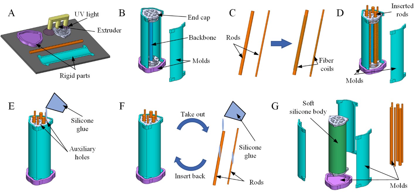
The silicone glue Ecoflex 00-10 was then used for the construction of the soft body of the arm section in the casting process and was injected into the mold from the axillary hole of one endcap. After the curing of the silicone glue, the rods for the cavities were extracted from the mold and were then inserted back with a silicone glue covering to construct an extra layer of silicone over the fiber coil for protection. Finally, all the mold pieces and the seal taps were removed and one section for the soft robotic arm was fabricated. After each section of the robotic arm was prepared, the actuation cables were first assembled with different sections. For each cable, one end was fixed on the endcap by using an anchor piece, and the other end was attached to the driving pulley. Screw connections were then applied to link different sections and the base for the whole robotic arm to complete the fabrication and assembling process of the prototype of the proposed soft robotic arm.
III Modeling of the Soft Robotic Arm
The kinematic model for the multi-section soft robotic arm is separated into two parts: a static model for a single section, which maps the actuation cable lengths to the bending configuration of one section; and another module that characterizes the relationship between the bending configurations for all sections and the task space variables (in particular, the end position of the arm).
III-A Static Model of a Section Driven by a Single Cable
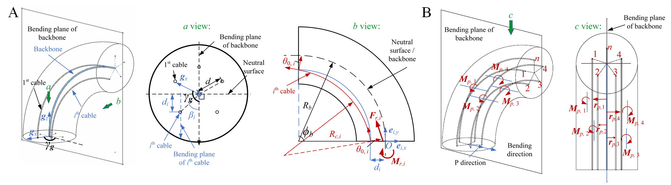
The static model for a single section of the robotic arm is built based on the analysis of its bending deformation. Before studying a section with multiple actuation cables, we consider the case with a single actuating cable and analyze an arbitrary bending configuration (Fig. 3A). The cable and the support of the section provide external forces. To simplify the static analysis, several assumptions are made:
(A1) The backbone (dash line) of the soft section has a constant length. (A2) The backbone and the cable (red line) have constant curvatures. (A3) The backbone has bending deformations within one single plane. (A4) The friction between the cables and the soft body of the arm is negligible. (A5) The soft section of the arm has a linear bending stiffness with no hysteresis. (A6) The cables have no slacks.
Refer to Fig. 3A. Let (subscript “b” for “backbone”) be the arclength parameter for the backbone. The bending angle of the section at a given point with an arclength is defined as the angle of rotation between the two local frames at the base, and at the point with on the backbone, , and can be described as:
| (1) |
where is the radius of the backbone curvature. The curvature of the backbone, , is written as:
| (2) |
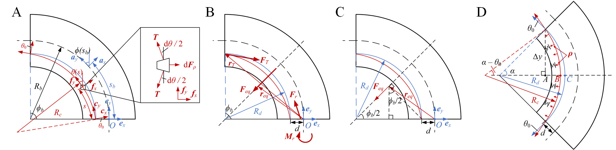
The curvature (subscript “c” for “cable”) for the cable is described similarly: , where is the radius of the actuation cable curvature, and is the arclength parameter for the cable. As illustrated in Fig. 3A, is the rotation angle between the base frame e and , where f is the local frame at the point with an arclength of on the cable.
Based on the force balance (Fig. 3A), the transverse force density between the cable and the soft body (Fig. 3D) is derived as:
| (3) |
| (4) |
where is the tension of the cable, is the transverse force between the cable and the soft body, is used to denote for simplicity, the notation “d” represents differential, and the relationship is used in the derivation of (3).
Another assumption following the introduction of is made to describe a simplified interaction model between the cable and the soft body of the arm:
(A7) The maximum transverse deformation of the cable ( in Fig. 3D) is proportional to the transverse force density applied by the cable (Fig. 3D).
Next, the transverse force density vector at point s, viewed in the base frame e (Fig. 3A), is calculated by using a rotation matrix :
| (5) |
| (6) |
The total transverse force (subscript “eq” for “equivalent total force”) between the cable and the soft body can then be obtained by the following integration:
| (7) | ||||
where is the cable length in the soft section, is the bending angle of the backbone at the tip, and is the incident angle of the cable, which is the angle between the tangent line (cy axis) of the cable at the base surface and the normal (ey axis) of the base surface (Fig. 3A, D).
The contraction force applied by the cable tip to the soft section (Fig. 3B) is calculated as:
| (8) |
From the force balance equation:
| (9) |
where Fr (subscript “r” for “reaction”) represents the support force applied by the base support of the soft section to the soft section (Fig. 3B), one can derive:
|
|
(10) |
Next, the moment balance of the section is analyzed with respect to the base point O (Fig. 3B). The arm (Fig. 3B) for is derived as:
| (11) | ||||
where is the radius of the cable curvature when the transverse deformation of the cable is not considered, is the distance between the incident point of the cable and the base point O of the section.
Since is located on the mirror-symmetric axis of the bending section (see Fig. 3C), the exact point of action of is irrelevant in computing the resulting moment around the point O; in other words, the moment is the same regardless of the point of action of . We have thus chosen the point of action as illustrated in Fig. 3C, with the associated arm vector represented as:
| (12) | ||||
From the moment the balance of the section:
| (13) |
where Mr denotes the support moment, and are the moments generated by and with respect to point O, respectively, and:
| (14) |
one obtains:
| (15) |
See the Appendix for calculation details of this concise result. Next, the incident angle of the cable (Fig. 3D) satisfies:
| (16) |
which implies:
| (17) |
where .
Based on assumption (A7) and the geometric relationships (Fig. 3D), one can obtain:
| (18) |
| (19) |
where is the maximum transverse deformation of the cable and is the coefficient in the simplified linear relationship between and .The physical interpretation of is the “cutting-in stiffness”, where the interaction between the normal force of the cable and the soft body is treated as a linear spring. Admittedly, the assumed linear relationship is a simplification, as the relationship could be nonlinear especially if the deformation is large. Despite the limitation, the experiment results later in the paper (see Fig. 8B) show that this model for the interaction between the cable and the soft body is adequately accurate to describe the transverse deformation phenomenon.
Based on assumption (A5), the relationship between the bending deformation and the external torque is derived by introducing a bending stiffness :
| (20) |
where is the internal elastic moment.
Finally, by using the equations (3), (15), (17-20), and the geometric relationships, the model for a single soft section driven by a single cable is captured by:
| (21) |
where is the length of the soft section’s backbone. In the forward mapping from actuation to the robotic arm configuration, the backbone curvature is solved based on the cable length by using a nonlinear equation set solver and numerical methods (e.g. “fsolve” in MATLAB), while in the inverse problem l is calculated based on a desired reference by using the nonlinear equation set solver. The incident angle , cable curvature and cable tension are intermediate variables, while , , , and are constants and , are dependent on . The initial guess for the solution to the nonlinear equations is derived by solving the last three equations in (21) when we assume that there is no transverse deformation of the cables (blue curve in Fig. 3A): .
III-B Static Model of a Section Driven by Multiple Cables
After the model for one section driven by one cable is obtained, the model for the case of a single section with multiple actuating cables is addressed, where we assume that there is no slack for any cable.
The bending configuration for the soft section with n evenly distributed cables (a general case) is defined by the bending angle and the bending orientation ( is with respect to the base frame g) (Fig. 4A). A curved neutral surface is defined so that it is perpendicular to the bending plane and contains the backbone. The cables are indexed counterclockwise and the direction of the x axis of the base frame g points to the 1st cable. The angle between the ith cable orientation (in the base plane) and the bending direction is written as (Fig. 4A):
| (22) |
where n is the total number of the evenly distributed cables in the soft section.
The distance between the incident point of the ith cable and the neutral plane is calculated as:
| (23) |
In the bending plane of the ith cable (Fig. 4A), which is parallel to the bending plane of the backbone and contains the ith cable, the external force condition is analyzed as the single cable-driven case:
|
|
(24) |
where, , and are the cable tension, incident angle and curvature of the ith cable, respectively, and and are the support force and moment components induced by the ith cable, respectively, in local frame (Fig. 4A).
Then, one can calculate the total bending moment applied by the cables for the section:
| (25) |
with:
| (26) |
Furthermore, since there is no bending deformation in the direction perpendicular to the bending direction, and based on assumption (A3), the total external moment applied by cables in the P direction with respect to O (Fig. 4B) is zero:
| (27) |
where is the external moment applied by the ith cable with respect to O, in the P direction.
The arm of the external forces for is the distance between the bending plane of the ith cable and the bending plane of the backbone (Fig. 4B), whose direction is perpendicular to the bending plane with the magnitude:
| (28) |
Thus, the lateral moment applied by the ith cable is derived as:
| (29) |
where , , and are the components along axis (or gz axis) of the , , and , respectively,
Then, based on equations (23)-(29) and the geometric relationships, the kinematic model for a soft section of the arm actuated by multiple cables is derived as:
|
|
(30) |
In the forward mapping from actuation to arm configuration, given the cable lengths , the backbone curvature and the bending orientation (manifested via in equation (22)) are obtained by solving the equation (30). , , and are intermediate variables, , , , and are constants, and , are fully determined by . Therefore, in the forward mapping problem, there are unknowns and independent equations. In the inverse mapping problem, the lengths for different cables are calculated based on the desired reference values of and by solving the same equation (30). It is noticed that (the number of the cables) is required to be larger than 2 to achieve a redundant actuation system for all of the bending orientations considering the limitation that is non-negative (in the inverse mapping, considering the equation (30), substituting by using , the numbers of independent equations and the unknown variables are and , respectively). The initial guess of the nonlinear system is obtained by solving the last three rows in (30), where we assume that there is no transverse deformation of the cables: .
III-C Modeling of a Multi-Section Soft Arm
For the multi-section soft robotic arm, the kinematic model between the task space configuration (in particular, the end position) and the bending configuration for each section is built by using homogeneous transformation matrices.25 Specifically, considering the thickness of the rigid endcaps, one can divide each section of the arm into three parts: straight, bending, and straight. The transformation matrix , which transforms vectors in the end frame to those in the base frame for the ith section (Fig. 5A), is given by:
|
|
(31) |
where and ( is with respect to a general base frame that is not dependent on the cable distribution) are the bending angle and orientation for the ith section, respectively, is the in-plane displacement from the base to tip for the ith section, is the curvature of the backbone of the ith section, is the displacement of the straight part and is the thickness of the endcaps. I is a three-dimensional identity matrix, , , and are the 3D rotation matrices around the z-axis, y-axis and z-axis for the angle , , and , respectively.
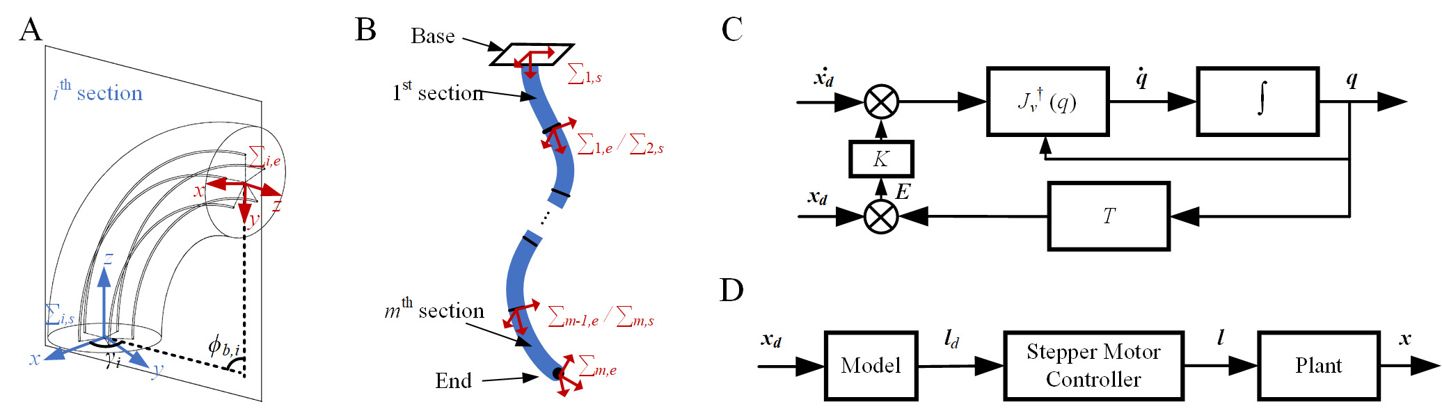
The transformation matrix which transforms vectors in the end frame to those in the base frame of the m-section arm, and the end position of the arm (subscript “t” for “tip”) in (Fig. 5B) can be calculated as:
| (32) |
| (33) |
where .
For the inverse kinematics,[41] the linear velocity Jacobian matrix for the end position of the m-section arm with respect to the variables of the bending configuration of each section is calculated as:
| (34) |
where is the set of variables of the bending configurations of all sections. The calculated is omitted for brevity and a small value is added to when for numerical stability. At least two sections are required for the arm to provide redundancy for tracking desired end positions in 3D space.
Once is obtained, one can use the following method to approach the configurations given the desired task space output (inverse kinematics) by using the pseudo-inverse of the Jacobian matrix :
| (35) |
| (36) |
where is an identity matrix, is a small positive number, is the velocity vector of the tracking trajectory (subscript “d” for “desired”), is any vector with the shape of and set to zero for the minimum energy criterium.
By using a numerical method to integrate the velocities, the references for the bending configuration variables are calculated:
| (37) |
where and denote at the time steps and , respectively.
Closed-loop feedback is further implemented (Fig. 5C) to reduce the error accumulated by the numerical integration in (37):
| (38) |
where is the feedback error and is a positive diagonal gain matrix. Once is obtained, we can use the equation (30) to calculate the cable lengths for different actuation cables for all sections.
IV Results
IV-A Baseline Model for the Soft Robotic Arm
Extensive experiments have been conducted to validate the proposed model. For comparison, an existing baseline model25 for the soft robotic arm is built, without considering the transverse deformation of the cable during bending. The multi-section part of the baseline kinematic model is the same as that of the proposed model, but the relationship between the cable lengths and the bending configuration of a single section is derived based on ideal geometrical relationships for the baseline model. In particular, the curvature and the length of the ith cable in a section (blue curve in Fig. 4A) is derived as:
| (39) |
| (40) |
where is derived from equation (23), and are the curvature and the length of the backbone, respectively.
IV-B Experiment Setups
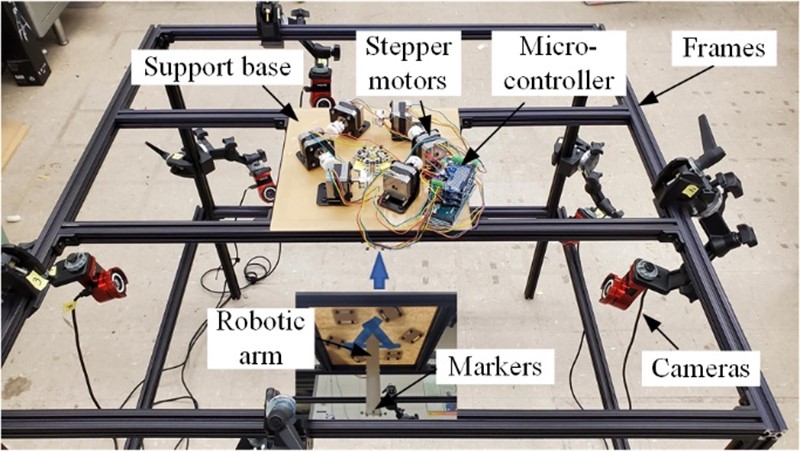
During the experiments for the soft robotic arm, 5 optical markers were attached at the end of the robotic arm to monitor the bending configuration and the end position of the robotic arm with a motion capture system (Fig. 6). The motion capture system used in the experiments was “Opti-track”, including a set of infrared cameras and the related software, which could track the position and orientation of the “Rigid Body” consisting of the attached markers on the robotic arm and provide accurate information for the bending angle , bending orientation , and the position for the end of the robotic arm.
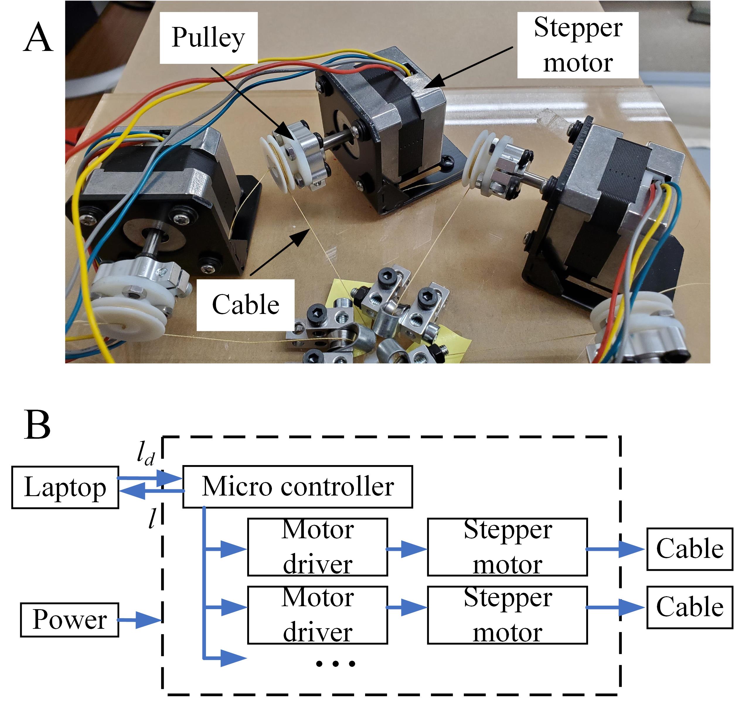
In the experiments, the cable length of the cables was controlled by using stepper motors, and the bending angle and orientation were recorded by the motion capture system. The actuation cable was driven by a 3D-printed pulley which was attached to a stepper motor (NEMA-17, Adafruit) (Fig. 7A). The stepper motors were controlled by a micro-controller (Arduino Mega 2560) in an open loop control (without encoder feedback) with the help of a stepper motor driver (Adafruit Motor Shield V2) for power amplification (Fig. 7B). Then, via serial communication, the microcontroller was communicated with a main controller (laptop), where the analytical models were computed before the reference for the stepper motor was sent out.
IV-C Parameter Identification
The geometric parameters () were measured directly from the prototype. The bending stiffness for a single section of the arm was calculated by using equations (15) and (20) assuming when was small, where and were measured by a force sensor and a motion capture system, respectively.
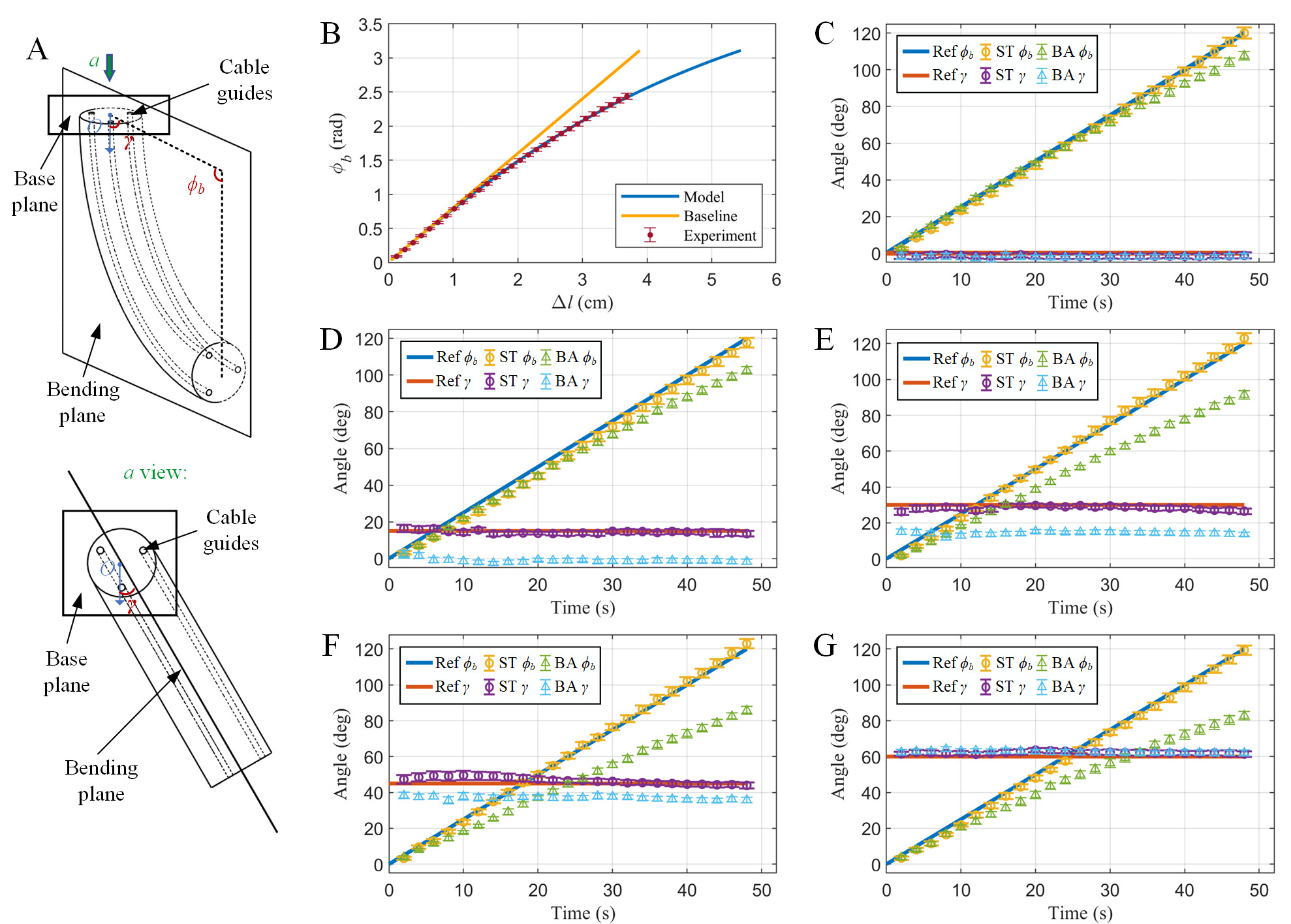
The relationship between a single cable contraction length and was obtained in the experiments for one soft section driven by a single cable to identify by using equation (21). In the experiments, the cable length of a single cable was controlled by using one stepper motor, and the bending angle was recorded by the motion capture system. The speeds of the stepper motors were controlled to be relatively slow for a quasi-static condition in all experiments. The contraction cable length were calculated after the experiments, and the experimental relationship between the and was obtained (Fig. 8B), based on which was identified.
The experiment results and the estimations based on the baseline model and the proposed model (equation (21)) with the identified parameters are shown in Fig. 8B. The error bars in experimental results represent the standard deviation of the result in three runs for each bending configuration. The identified parameters of the one section for the soft robotic arm used in the experiments are shown in the Table 1.
| Parameters | ||||
|---|---|---|---|---|
| Values | 9.30 | 1.25 | 20.02 | 3.10 |
IV-D Experimental Results for a Single Section
The single cable actuation results (Fig. 8B) showed that, compared with the baseline model, the proposed kinematic model was better in describing the nonlinear relationship between the cable actuation and the bending angle for the soft robotic arm, especially when the cable contraction length was relatively large.
After the model parameters were identified, extensive experiments were conducted to compare the accuracy of the baseline model and the proposed static model (equation (30)), where an open loop control without feedback was used (Fig. 5D). A single section of the robotic arm was used to track different bending angles in specific bending orientations by using different models (Fig. 8A). The bending orientation was sampled within 0 to 60 degrees becasue of the structural symmetry.
The cable actuation and control system as aforementioned was used for the multi-cable actuation experiments, where three and six motors were used for the single and the two section robotic arm, respectively. A simple and effective actuation strategy was used to deal with the multi-cable redundancy in each section and simplify the calculation of the static model: The tension of the cable , that had the largest angle between the cable orientation and the bending direction, was set to be 0 in the static model calculation (made it to be "slack").
| (41) |
During the experiments, the target cable lengths were firstly calculated by using the kinematic model and the bending angle references with the help of the nonlinear system solver “” in MATLAB. Then, the target cable lengths were sent to the microcontroller and converted into the references for the rotation positions of the stepper motors. Finally, the microcontroller drove the stepper motors to reach the target rotation position and actuated the cables, where the speeds of the stepper motors were controlled to be relatively slow for a quasi-static condition. The error bars in the experimental results represent the standard deviations of the results in three identical trials.
The experiment results of the bending configurations (, ) of the single section arm controlled by multiple cables by using different models are shown in Fig. 8C-G. In the experiments, it was shown that the tracking accuracy of the proposed static model was significantly better compared to the baseline model in the experimental range (Fig. 8C-G), indicating the importance of considering the transverse deformation of the cable in the proposed robotic arm. In particular, the tracking errors in and were small for different bending configurations when the proposed model was used. In comparison, the tracking error in for the baseline model increased together with the target when the target was fixed, while the tracking error in for the baseline model was almost constant despite the changing of the target when the target was fixed.
Moreover, it was also shown that in the experiment range, the tracking error in for the baseline model increased with larger target when the target was fixed. The maximum tracking error increased from about 12 degrees to about 37 degrees when the target increased from 0 to 60 degrees, respectively. The tracking error for the baseline model increased from about 0 to about 16 degrees when the target increased from 0 to 30 degrees, respectively, and then decreased to near 0 when the target increased to 60 degrees. It was noticed that for both models, the tracking error approached 0 when target was 0 and 60 degrees, which was attributed to a single effective cable contraction and two effective cable contractions with the same contraction length, respectively, making the tracking error increased and then decreased in the experimental range. Specifically, when the target was 0 degree, there was only one effective actuation cable (the other two cable were almost slack) for both the baseline model and the proposed model, and the bending orientation in the experiment naturally stayed around 0 degree, which was the same as the orientation of the actuation cable. When the target was 60 degrees, the two actuation cables shared the same contraction length (the third cable was almost slack) for both the baseline model and proposed model, and in the experiment stayed near 60 degrees because of the actuation and structure symmetry.
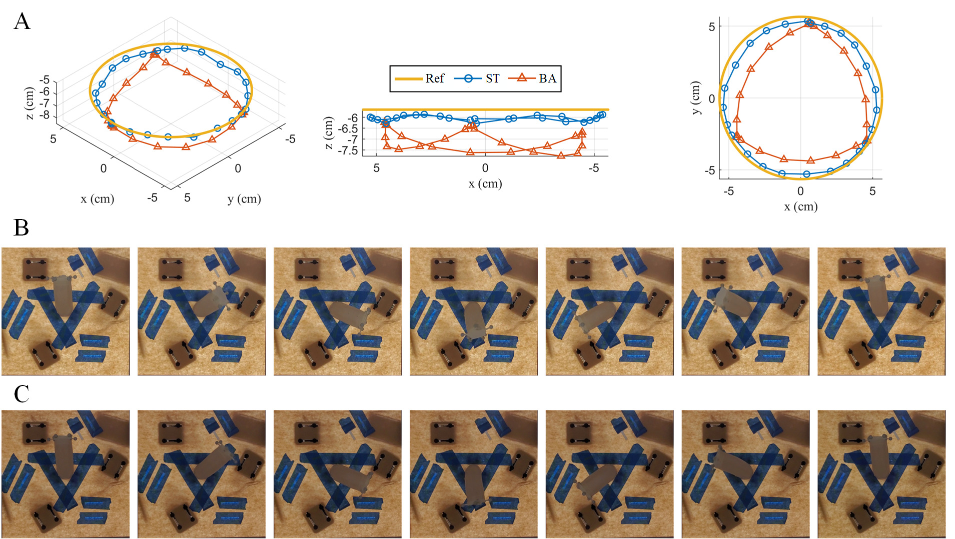
A trajectory tracking experiment for the endpoint of the single section was further conducted where the trajectory reference was included in the workspace of the single section. The experiment showed that the average tracking error of the single section (1.58 cm) by using the proposed model (equation (30)) was about 35% smaller than that (2.43 cm) of the baseline model (Fig. 9A), and the soft section had flexible and versatile bending configurations (Fig. 9B-C). More experiment results for the trajectory tracking experiments for the single section arm showed the repeatability of the tests and the effusiveness of the model (Fig. A1 in Appendix). A video of these experiments and those in Section IV-E can be viewed at https://youtu.be/I-e1PxHwG1Y.
IV-E Experimental Results for a Two-Section Soft Robotic Arm
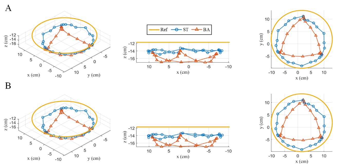
A multi-section arm was assembled and utilized for the comparison of the baseline model and the proposed model, and its performance was further evaluated. For simplicity, a two-section arm was assembled and controlled to track a circular trajectory within its workspace by using the baseline model and the proposed model. The experiment results showed that, the average tracking error with the proposed model (3.76 cm) was about 36% smaller compared with the baseline model (5.92 cm), and the trajectory achieved with the controller based on the proposed model was closer to the reference (Fig. 10A-C). Compared with the tracking error when using a single section, the tracking error of the two-section soft arm was larger, which might be attributed to the error accumulation of multiple sections and a more prominent gravity influence for the base section of the soft arm.
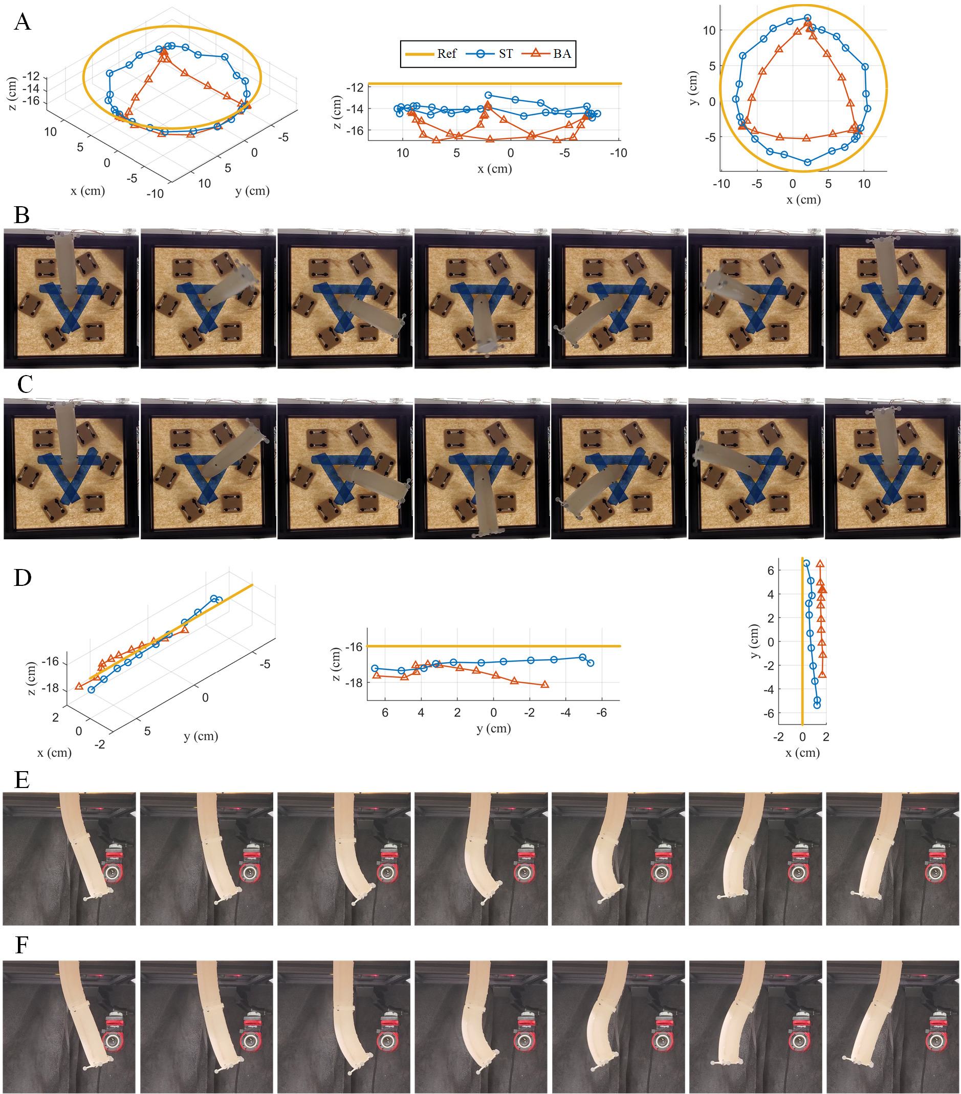
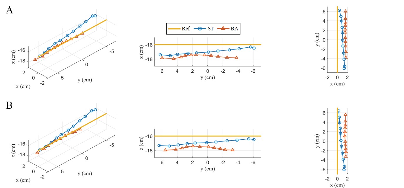
In addition, the two-section arm was controlled to track a straight trajectory within its workspace by using the two different models, where the average tracking error (1.70 cm) of the proposed model was about 52% smaller than that of the baseline model (3.52 cm) (Fig. 10D-F). In summary, the extensive experiments showed the advantage of the proposed kinematic model as compared to the geometric baseline model and validated the flexibility and dexterity of the proposed soft robotic arm.
More experiment results for the trajectory tracking experiments for the two section arm showed the repeatability of the tests and the effusiveness of the model (Fig. A2, A3 in Appendix).
V Discussion and Conclusion
In this work, we designed an octopus-inspired soft robotic arm and developed a novel kinematic model to characterize its flexible movements. The modular design of the soft arm enabled longer arm prototypes and permitted a decoupling cable actuation system for different sections that simplified the modeling. The hybrid fabrication method of 3D printing and casting resulted in low-cost and easy-to-build prototypes. An analytical static model was built to capture the transverse deformation of the cable during actuation, which was largely ignored in the literature.
Extensive experiments were conducted to validate the proposed model and a geometric baseline model was used for comparison. The results of tracking experiments for a single section of the soft arm showed an evident advantage and smaller tracking errors for the proposed model over the baseline model in terms of bending angle, orientation, and the end position of the arm. Experiments with a two-section arm further supported the efficiency of the proposed model in tracking circular and straight trajectories for the endpoint and demonstrated the dexterity of the proposed soft arm.
We note that our modeling approach was not only motivated by and particularly relevant to the proposed modular soft robotic arm, but also applicable to many other cable-driven robotic arms, especially those not using rigid spacers, examples of which are abundant [42, 43, 44]. Even for cable-driven soft robotic arms with multiple rigid spacers, the transverse deformation phenomenon would still exist in the sections between the rigid spacers where the cables and the soft body interact directly.
For future work, we will extend the analytical model for the proposed soft robotic arm in several directions. First, in this work we used the PCC assumption, which would hold only in the absence of pronounced gravity effect and external forces. We plan to improve the model by considering the moments introduced by the gravity and external forces, using an iterative approach similar to the modeling of a soft pneumatic actuator by Fairchild et al.[45] In particular, one can first use the model presented in this paper to obtain the constant curvature for each section in the absence of the gravity and external forces — or equivalently, the “actuation moment” that is uniform throughout the section. Then the moments induced by the gravity and external forces can be evaluated based on that curvature, and these moments (along with the “actuation moment”) are used to update the curvature (now non-constant). This process can repeat until the curvature function converges. We will also explore the related dynamic model with external interactions. Finally, we will develop integrated embedded sensors (e.g., soft strain sensors) for the soft robotic arm, so that real-time bending configuration data for each section of the arm are made available for feedback control.
References
- [1] Z. Gong, X. Fang, X. Chen, et al., “A soft manipulator for efficient delicate grasping in shallow water: Modeling, control, and real-world experiments,” The International Journal of Robotics Research, vol. 40, no. 1, pp. 449–469, 2021.
- [2] Z. Xie, A. G. Domel, N. An, et al., “Octopus arm-inspired tapered soft actuators with suckers for improved grasping,” Soft robotics, vol. 7, no. 5, pp. 639–648, 2020.
- [3] L. Zongxing, L. Wanxin, and Z. Liping, “Research development of soft manipulator: A review,” Advances in Mechanical Engineering, vol. 12, no. 8, p. 1687814020950094, 2020.
- [4] C. Lee, M. Kim, Y. J. Kim, et al., “Soft robot review,” International Journal of Control, Automation and Systems, vol. 15, pp. 3–15, 2017.
- [5] P. Palmieri, M. Melchiorre, and S. Mauro, “Design of a lightweight and deployable soft robotic arm,” Robotics, vol. 11, no. 5, p. 88, 2022.
- [6] X. Liang, H. Cheong, Y. Sun, J. Guo, C. K. Chui, and C.-H. Yeow, “Design, characterization, and implementation of a two-dof fabric-based soft robotic arm,” IEEE Robotics and Automation Letters, vol. 3, no. 3, pp. 2702–2709, 2018.
- [7] X. Wang, H. Kang, H. Zhou, W. Au, M. Y. Wang, and C. Chen, “Development and evaluation of a robust soft robotic gripper for apple harvesting,” Computers and Electronics in Agriculture, vol. 204, p. 107552, 2023.
- [8] M. Wu, X. Zheng, R. Liu, N. Hou, W. H. Afridi, R. H. Afridi, X. Guo, J. Wu, C. Wang, and G. Xie, “Glowing sucker octopus (stauroteuthis syrtensis)-inspired soft robotic gripper for underwater self-adaptive grasping and sensing,” Advanced Science, vol. 9, no. 17, p. 2104382, 2022.
- [9] M. Cianchetti, T. Ranzani, G. Gerboni, I. De Falco, C. Laschi, and A. Menciassi, “Stiff-flop surgical manipulator: Mechanical design and experimental characterization of the single module,” in 2013 IEEE/RSJ international conference on intelligent robots and systems, pp. 3576–3581, IEEE, 2013.
- [10] A. Diodato, M. Brancadoro, G. De Rossi, et al., “Soft robotic manipulator for improving dexterity in minimally invasive surgery,” Surgical innovation, vol. 25, no. 1, pp. 69–76, 2018.
- [11] Z. Wang, S. Hirai, and S. Kawamura, “Challenges and opportunities in robotic food handling: A review,” Frontiers in Robotics and AI, vol. 8, p. 789107, 2022.
- [12] X. Chen, X. Zhang, Y. Huang, L. Cao, and J. Liu, “A review of soft manipulator research, applications, and opportunities,” Journal of Field Robotics, vol. 39, no. 3, pp. 281–311, 2022.
- [13] J. Walker, T. Zidek, C. Harbel, S. Yoon, F. S. Strickland, S. Kumar, and M. Shin, “Soft robotics: A review of recent developments of pneumatic soft actuators,” in Actuators, vol. 9, p. 3, MDPI, 2020.
- [14] X. Qi, H. Shi, T. Pinto, and X. Tan, “A novel pneumatic soft snake robot using traveling-wave locomotion in constrained environments,” IEEE Robotics and Automation Letters, vol. 5, no. 2, pp. 1610–1617, 2020.
- [15] Z. Xing, J. Zhang, D. McCoul, Y. Cui, L. Sun, and J. Zhao, “A super-lightweight and soft manipulator driven by dielectric elastomers,” Soft robotics, vol. 7, no. 4, pp. 512–520, 2020.
- [16] I. A. Anderson, T. A. Gisby, T. G. McKay, B. M. O’Brien, and E. P. Calius, “Multi-functional dielectric elastomer artificial muscles for soft and smart machines,” Journal of applied physics, vol. 112, no. 4, 2012.
- [17] H. Yang, M. Xu, W. Li, and S. Zhang, “Design and implementation of a soft robotic arm driven by sma coils,” IEEE Transactions on Industrial Electronics, vol. 66, no. 8, pp. 6108–6116, 2018.
- [18] C. Laschi, M. Cianchetti, B. Mazzolai, L. Margheri, M. Follador, and P. Dario, “Soft robot arm inspired by the octopus,” Advanced robotics, vol. 26, no. 7, pp. 709–727, 2012.
- [19] Y. Kim, G. A. Parada, S. Liu, and X. Zhao, “Ferromagnetic soft continuum robots,” Science Robotics, vol. 4, no. 33, p. eaax7329, 2019.
- [20] C. Li and C. D. Rahn, “Design of continuous backbone, cable-driven robots,” J. Mech. Des., vol. 124, no. 2, pp. 265–271, 2002.
- [21] W. Dou, G. Zhong, J. Cao, Z. Shi, B. Peng, and L. Jiang, “Soft robotic manipulators: Designs, actuation, stiffness tuning, and sensing,” Advanced Materials Technologies, vol. 6, no. 9, p. 2100018, 2021.
- [22] T. Deng, H. Wang, W. Chen, X. Wang, and R. Pfeifer, “Development of a new cable-driven soft robot for cardiac ablation,” in 2013 IEEE International Conference on Robotics and Biomimetics (ROBIO), pp. 728–733, IEEE, 2013.
- [23] S. M. Mustaza, Y. Elsayed, C. Lekakou, C. Saaj, and J. Fras, “Dynamic modeling of fiber-reinforced soft manipulator: A visco-hyperelastic material-based continuum mechanics approach,” Soft robotics, vol. 6, no. 3, pp. 305–317, 2019.
- [24] Q. Xie, T. Wang, and S. Zhu, “Simplified dynamical model and experimental verification of an underwater hydraulic soft robotic arm,” Smart Materials and Structures, vol. 31, no. 7, p. 075011, 2022.
- [25] R. J. Webster III and B. A. Jones, “Design and kinematic modeling of constant curvature continuum robots: A review,” The International Journal of Robotics Research, vol. 29, no. 13, pp. 1661–1683, 2010.
- [26] D. B. Camarillo, C. F. Milne, C. R. Carlson, M. R. Zinn, and J. K. Salisbury, “Mechanics modeling of tendon-driven continuum manipulators,” IEEE transactions on robotics, vol. 24, no. 6, pp. 1262–1273, 2008.
- [27] D. B. Camarillo, C. R. Carlson, and J. K. Salisbury, “Configuration tracking for continuum manipulators with coupled tendon drive,” IEEE transactions on robotics, vol. 25, no. 4, pp. 798–808, 2009.
- [28] F. Renda, M. Giorelli, M. Calisti, M. Cianchetti, and C. Laschi, “Dynamic model of a multibending soft robot arm driven by cables,” IEEE Transactions on Robotics, vol. 30, no. 5, pp. 1109–1122, 2014.
- [29] T. Morales Bieze, A. Kruszewski, B. Carrez, and C. Duriez, “Design, implementation, and control of a deformable manipulator robot based on a compliant spine,” The International Journal of Robotics Research, vol. 39, no. 14, pp. 1604–1619, 2020.
- [30] S. Grazioso, G. Di Gironimo, and B. Siciliano, “A geometrically exact model for soft continuum robots: The finite element deformation space formulation,” Soft robotics, vol. 6, no. 6, pp. 790–811, 2019.
- [31] D. Trivedi, A. Lotfi, and C. D. Rahn, “Geometrically exact models for soft robotic manipulators,” IEEE Transactions on Robotics, vol. 24, no. 4, pp. 773–780, 2008.
- [32] F. Xu, H. Wang, K. W. S. Au, W. Chen, and Y. Miao, “Underwater dynamic modeling for a cable-driven soft robot arm,” IEEE/ASME transactions on Mechatronics, vol. 23, no. 6, pp. 2726–2738, 2018.
- [33] D. C. Rucker and R. J. Webster III, “Statics and dynamics of continuum robots with general tendon routing and external loading,” IEEE Transactions on Robotics, vol. 27, no. 6, pp. 1033–1044, 2011.
- [34] F. Renda, C. Armanini, V. Lebastard, F. Candelier, and F. Boyer, “A geometric variable-strain approach for static modeling of soft manipulators with tendon and fluidic actuation,” IEEE Robotics and Automation Letters, vol. 5, no. 3, pp. 4006–4013, 2020.
- [35] F. Renda, C. Armanini, A. Mathew, and F. Boyer, “Geometrically-exact inverse kinematic control of soft manipulators with general threadlike actuators’ routing,” IEEE Robotics and Automation Letters, vol. 7, no. 3, pp. 7311–7318, 2022.
- [36] F. Renda, F. Boyer, J. Dias, and L. Seneviratne, “Discrete cosserat approach for multisection soft manipulator dynamics,” IEEE Transactions on Robotics, vol. 34, no. 6, pp. 1518–1533, 2018.
- [37] Y. Wu, J. K. Yim, J. Liang, Z. Shao, M. Qi, J. Zhong, Z. Luo, X. Yan, M. Zhang, X. Wang, et al., “Insect-scale fast moving and ultrarobust soft robot,” Science robotics, vol. 4, no. 32, p. eaax1594, 2019.
- [38] H. R. Choi, K. Jung, S. Ryew, J.-D. Nam, J. Jeon, J. C. Koo, and K. Tanie, “Biomimetic soft actuator: design, modeling, control, and applications,” IEEE/ASME transactions on mechatronics, vol. 10, no. 5, pp. 581–593, 2005.
- [39] X. Qi, T. Gao, and X. Tan, “Bioinspired 3d-printed snakeskins enable effective serpentine locomotion of a soft robotic snake,” Soft Robotics, vol. 10, no. 3, pp. 568–579, 2023.
- [40] S. Kim, C. Laschi, and B. Trimmer, “Soft robotics: a bioinspired evolution in robotics,” Trends in biotechnology, vol. 31, no. 5, pp. 287–294, 2013.
- [41] L. Sciavicco and B. Siciliano, Modelling and control of robot manipulators. Springer Science & Business Media, 2001.
- [42] H. Wang, W. Chen, X. Yu, T. Deng, X. Wang, and R. Pfeifer, “Visual servo control of cable-driven soft robotic manipulator,” in 2013 IEEE/RSJ International Conference on Intelligent Robots and Systems, pp. 57–62, IEEE, 2013.
- [43] T. Deng, H. Wang, W. Chen, X. Wang, and R. Pfeifer, “Development of a new cable-driven soft robot for cardiac ablation,” in 2013 IEEE International Conference on Robotics and Biomimetics (ROBIO), pp. 728–733, IEEE, 2013.
- [44] W. Dou, G. Zhong, J. Cao, Z. Shi, B. Peng, and L. Jiang, “Soft robotic manipulators: Designs, actuation, stiffness tuning, and sensing,” Advanced Materials Technologies, vol. 6, no. 9, p. 2100018, 2021.
- [45] P. Fairchild, N. Shepard, Y. Mei, and X. Tan, “Semi-physical modeling of soft pneumatic actuators with stiffness tuning,” ASME Letters in Dynamic Systems and Control, pp. 1–6, 2023.
-A Supplementary Derivations for Modeling of Soft Robotic Arm
The detailed derivation for the equation (14) is as follows: We can first denote and , then we can derive:
where is calculated as:
Thus, finally we can derive:
which shows an elegant result of the external moment applied to the single section of the cable driven robotic arm.
-B Supplementary Results for Trajectory Tracking Experiments
More trajectory tracking experiments were conducted for the proposed soft robotic (Fig. A1-A3). Two more sets of experiments were conducted for a single section of the soft arm tracking the circular trajectory (Fig. A1A-B), which shared the same experiment settings as the experiments in Fig. 9. The result of the supplementary experiment set 1 showed that the average tracking error of the single section by using the proposed model (1.55 cm) was about 49 smaller than that of the baseline model (3.06 cm) (Fig. A1A). The result of the supplementary experiment set 2 showed that the average tracking error of the single section by using the proposed model (1.57 cm) was about 43 smaller than that of the baseline model (2.75 cm) (Fig. A1B). The supplementary experiment sets demonstrated similar results as the trajectory tracking results of the experiments in Fig. 9 and showed their reproducibility.
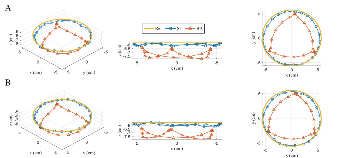
Furthermore, two more sets of experiments were conducted for the two-section soft robotic arm tracking the circular trajectory (Fig. A2A-B) and the straight trajectory (Fig. A3A-B), where the experiment settings remained the same as those in the main text. In the experiments tracking the circular trajectory, the average tracking error with the proposed model (3.88 cm) was about 36 smaller compared with the baseline model (6.02 cm) (Fig. A2A) in the supplementary experiment set 1. For the supplementary experiment set 2, the average tracking error with the proposed model (3.84 cm) was about 35 smaller compared with the baseline model (5.93 cm) (Fig. A2B). The supplementary experiment sets demonstrated similar results as the trajectory tracking results of the experiments in Fig. 10A and showed their reproducibility.
In the experiments tracking the straight trajectory, the average tracking error with the proposed model (1.77 cm) was about 41 smaller compared with the baseline model (2.98 cm) (Fig. A3A) in the supplementary experiment set 1. For the supplementary experiment set 2, the average tracking error with the proposed model (1.57 cm) was about 47 smaller compared with the baseline model (2.96 cm) (Fig. A3B). The supplementary experiment sets demonstrated similar results as the trajectory tracking results of the experiments in Fig. 10D and showed their reproducibility.