Enhancing a Convolutional Autoencoder with a Quantum Approximate Optimization Algorithm for Image Noise Reduction

Abstract

Image denoising is essential for removing noise in images caused by electric device malfunctions or other factors during image acquisition. It helps preserve image quality and interpretation. Many convolutional autoencoder algorithms have proven effective in image denoising. Owing to their promising efficiency, quantum computers have gained popularity. This study introduces a quantum convolutional autoencoder (QCAE) method for improved image denoising. This method was developed by substituting the representative latent space of the autoencoder with a quantum circuit. To enhance efficiency, we leveraged the advantages of the quantum approximate optimization algorithm (QAOA)-incorporated parameter-shift rule to identify an optimized cost function, facilitating effective learning from data and gradient computation on an actual quantum computer. The proposed QCAE method outperformed its classical counterpart as it exhibited lower training loss and a higher structural similarity index (SSIM) value. QCAE also outperformed its classical counterpart in denoising the MNIST dataset by up to 40% in terms of SSIM value, confirming its enhanced capabilities in real-world applications. Evaluation of QAOA performance across different circuit configurations and layer variations showed that our technique outperformed other circuit designs by 25% on average.

1 Introduction

Images acquired from image sensors frequently exhibit noise caused by hardware malfunctions and various environmental factors. In this context, noise denotes unpredictable fluctuations in brightness, intensity, or color information within a digital image [11, 33]. Image denoising is pivotal for eliminating these distortions from a given input image, aiming to generate a more refined and clearer image [12, 21]. The denoising process is essential for accurate image analysis and benefits both human interpretation and machine learning (ML)-based assessments [46]. ML-based methods comprise supervised, semisupervized, and unsupervised learning methods [26].

An autoencoder (AE) stands out as an unsupervised learning model designed for input reconstruction using a neural network (NN) model. This class of models demonstrates notable versatility, particularly in the group of learning representations [2]. AEs encompass numerous successful variants, including the variational autoencoder (VAE), convolutional autoencoder (CAE), and denoising autoencoder, as discussed in [37]. They operate by mapping the input to a lower-dimensional space (latent space). These encoding and decoding steps are subsequently used to accurately reconstruct the original image. However, the latent space in AE encounters challenges in accurately capturing complex, nonlinear relationships among data points. Moreover, it prioritizes common data points, leaving gaps in the latent space for less frequent data samples and limiting diversity and usability for tasks such as regeneration.

Recently, the popularity of quantum computers has surged among researchers, driven by their unique computational capabilities, such as superposition. Superposition allows quantum circuits to represent multiple states simultaneously, enabling them to model the complex, nonlinear relationships that classical systems struggle with. This capability can lead to more accurate and efficient data compression than classical AE. However, quantum computers remain suboptimal for production applications [6]. The existing quantum computing (QC) landscape is in the noisy intermediate-scale quantum (NISQ) era [5], indicating that current quantum systems exhibit limitations in terms of the number of qubits, circuit depth, and high noise levels. Because of these factors, variational quantum algorithms (VQAs) have emerged as an ideal choice for implementation, primarily due to their lower qubit requirements and reduced circuit depth. VQAs leverage classical computation to optimize the algorithm parameters effectively [18]. In addition, they exhibit robustness against image noise - a major problem for other types of quantum algorithms. The quantum approximate optimization algorithm (QAOA), a leading VQA, tackles combinatorial optimization by transforming the problem into finding the ground state of its corresponding Hamiltonian.

Due to exponentially increasing computational power and the ability to learn data representations in higher-dimensional spaces, our primary objective in this study is to integrate CAE and QAOA to create an advanced latent space for execution within QC. We enhanced our model by incorporating a trainable quantum variational circuit to develop a hybrid architecture termed a quantum convolutional autoencoder (QCAE). The QCAE was specifically designed for the task of MNIST image denoising. To showcase its efficacy, we conducted a comparative analysis of its performance against its classical counterpart, the classical convolutional autoencoder (CCAE). The contributions of this study are as follows:

• We present an approach that combines a convolutional autoencoder network with quantum circuits to tackle image denoising efficiently. This integration provides the benefit of using a reduced number of qubits, rendering it particularly well-suited for current NISQ devices.

• We leverage the QAOA to replace the classical latent space, elevating the input into a higher-dimensional space. This transformation enhances the representation of data, leading to improved accuracy and effectiveness, as QAOA is used to find the minimum objective function (cost function).

• We leverage an advanced parameter-shift rule (PSR) technique to optimize the QAOA parameters finely, resulting in a substantial improvement in the effectiveness of image denoising through this dual parameter shifting strategy.

• We rigorously conducted denoising experiments using the MNIST dataset, exploring diverse image noise factors across both quantum simulation and machine scenarios. This comprehensive study aims to refine and advance denoising techniques applied to a widely used MNIST dataset.

The rest of the paper is organized as follows. Section 2 describes both classical and quantum algorithms for image denoising and classification. Section 3 reviews the associated background to understand this paper. In Section 4, we delve into the intricate details of our proposed methodology, leveraging QAOA in conjunction with PSR optimization. Section 5 details the specifics of the dataset and environments employed in our study. In Section 6, we present a comprehensive showcase of our superior performance in image denoising. Finally, Section 7 concludes the paper.

2 Related works

In the field of classical image denoising, deep learning serves as the main building block, harnessing the power of neural networks (NN) to effectively reduce noise and enhance image quality. Gondara et al. [15] demonstrated that denoising AE, constructed with convolutional layers and applied to small sample sizes, proves to be an effective solution for efficiently denoising medical images. The experiment reveals that even the most basic networks can successfully reconstruct images, even in the presence of corruption levels so severe that the distinction between noise and signal becomes imperceptible to the human eye. Venkataraman et al. [45] employed a straightforward AE network, constructing various architectures for the model. They systematically compared the results to determine the most suitable architecture for image denoising. Paul et al. [32] introduced an efficient denoising method for hyperspectral images (HSI), targeting various noise patterns and their combinations. Using a dual-branch deep neural network based on wavelet-transformed bands, the first branch uses convolutional layers with residual learning for local and global noise feature extraction. The second branch contains an AE layer with subpixel sampling for prominent noise feature extraction. Schneider et al. [39] implemented a CAE, a VAE, and an adversarial autoencoder on two distinct publicly available datasets. Subsequently, we conducted a comprehensive comparison of their anomaly-detection performance. In [38], the author extensively reviewed medical denoising techniques for images, emphasizing their significant importance in medical applications, particularly in disease diagnosis.

Numerous studies leverage QC and NN to develop image classification and denoising. Bravo et al. [7] presented an enhanced feature quantum autoencoder, a VQA capable of compressing the quantum states of different models with higher fidelity. They validated the method in simulations by compressing the ground states of the Ising model and classical MNIST handwritten digits. Although this approach effectively compressed and reconstructed images, its primary design did not prioritize the task of denoising images. Rivas et al. [35] presented a hybrid QML approach for representation learning. They utilized a quantum variational circuit that could be trained using conventional gradient descent techniques. To further enhance its performance, the method dressed the quantum circuit with AE layers for meaningful interpretation of complex unstructured data. Orduz et al. [29] applied randomized quantum circuits to process input data, functioning as quantum convolutions to generate representations applicable in convolutional networks. The experimental findings indicate comparable performance to traditional convolutional neural networks, with quantum convolutions demonstrating potential acceleration in convergence in certain scenarios. Nguyen et al. [27] used a D-Wave 2X quantum computer to address NP-hard sparse coding problems in image classification. The method involves downsampling MNIST images, employing a bottleneck autoencoder, and using quantum inference on D-Wave 2X to obtain sparse binary representations. The study also explored lateral inhibition between features generated from a subset of autoencoder-reduced MNIST images. Sleeman et al. [42] proposed a hybrid system that integrates a classical AE with a quantum annealing restricted Boltzmann machine (RBM) on a D-Wave quantum computer. The system achieved a nearly 22-fold compression of grayscale images to binary with lossy recovery. The evaluation of the MNIST dataset demonstrated the feasibility of using D-Wave as a sampler for ML. Additionally, the study compared the results of a hybrid quantum RBM with a hybrid classical RBM in a downstream classification problem and measured image similarity between MNIST-generated images and the original training dataset.

3 Preliminaries

In this section, we introduce the basics of QC and its data processing. We then explore how quantum computers handle classical data, discuss the execution of parameterized circuit data, and present the foundation of CCAE as our proposed method counterpart.

3.1 Quantum computing (QC)

QC harnesses the extraordinary principles of quantum physics, including superposition, entanglement, and quantum measurement, to accelerate data processing capabilities exponentially [40]. This section describes the fundamental and pivotal elements that empower quantum computers.

3.1.1 Quantum bit (Qubit)

The operational architecture of quantum computers differs fundamentally from that of classical computers. Quantum computers use quantum bits (qubits) as operational units, unlike classical computers, which rely on binary digits existing in either states 0 or 1. A qubit can exist simultaneously in a superposition of states 0, 1, and a linear combination of both 0 and 1 [28]. A qubit is defined as a linear combination of $|0\rangle$ and $|1\rangle$ which are eigen states of SU(2) Hermitian Hamiltonian as follows:

$$|0\rangle=\begin{bmatrix}1\\ 0\end{bmatrix},\;|1\rangle=\begin{bmatrix}0\\ 1\end{bmatrix},\;|\psi\rangle=\alpha|0\rangle+\beta|1\rangle=\begin{bmatrix}\alpha\\ \beta\end{bmatrix},$$ (1)

where the probability coefficients $\alpha$ and $\beta$ are called amplitudes. The sum of the squared amplitudes in a superposition equals 1, which is ${|\alpha|}^{2}+{|\beta|}^{2}=1$. Despite the ability of qubits to exist simultaneously in both $|0\rangle$ and $|1\rangle$ states, their definitive output is determined as either $|0\rangle$ or $|1\rangle$ when measured.

3.1.2 Quantum data manipulation

Data on a qubit can be transformed and manipulated using quantum gates. These quantum gates fundamentally involve the modification of one or more qubits [43]. The gates introduced in this paper include Hardamard ($H$), CNOT, and rotation gates such as X-rotation ($R_{X}$), Y-rotation ($R_{Y}$), and Z-rotation ($R_{Z}$). They are defined as follows:

$$\begin{array}[]{L}H=\frac{1}{\sqrt{2}}\begin{bmatrix}1&1\\ 1&-1\end{bmatrix},\quad CNOT=\begin{bmatrix}1&0&0&0\\ 0&1&0&0\\ 0&0&0&1\\ 0&0&1&0\\ \end{bmatrix},\end{array}$$ (2)

$$R_{X}(\theta)=\begin{bmatrix}cos\Bigl{(}\frac{\theta}{2}\Bigl{)}&-i\cdot sin\Bigl{(}\frac{\theta}{2}\Bigl{)}\\ \\ -i\cdot sin\Bigl{(}\frac{\theta}{2}\Bigl{)}&cos\Bigl{(}\frac{\theta}{2}\Bigl{)}\end{bmatrix},$$ (3)

$$R_{Y}(\theta)=\begin{bmatrix}cos\Bigl{(}\frac{\theta}{2}\Bigl{)}&-sin\Bigl{(}\frac{\theta}{2}\Bigl{)}\\ \\ sin\Bigl{(}\frac{\theta}{2}\Bigl{)}&cos\Bigl{(}\frac{\theta}{2}\Bigl{)}\end{bmatrix},$$ (4)

$$R_{Z}(\theta)=\begin{bmatrix}e^{-i\frac{\theta}{2}}&0\\ 0&e^{i\frac{\theta}{2}}\end{bmatrix}.$$ (5)

All gates except CNOT are single-qubit gates. The $H$ gate enables the creation of a superposition for a single qubit, while rotation gates allow a qubit to be positioned at any point on a Bloch sphere surface. However, CNOT is a two-qubit gate that facilitates entanglement between two qubits. These gates collectively enable quantum state manipulation.

3.2 Classical data encoding

Numerous QML algorithms require converting classical data into quantum states within quantum computers, a process known as data encoding [9, 48]. In other words, the dataset is initially translated from the subject data domain $D$ to the Hilbert space $H$ through a designated feature mapping process $f:D\rightarrow H$. One of the encoding techniques, specifically angle encoding or qubit encoding, is widely renowned for its ability to leverage a minimal number of qubits that correspond to the size of the input vector [30]. The angle encoding scheme demonstrates remarkable efficiency as it necessitates the rotation of only a single qubit as depicted in Fig. 1.

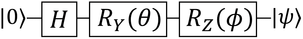
Figure 1: Angle encoding quantum circuit.

In this technique, each data value $x$ undergoes an initial normalization process, mapping it to the range $[0,2\pi]$. Subsequently, it is encoded using single-qubit rotation gates $R_{X}$, $R_{Y}$, and $R_{Z}$. These rotation gates dynamically determine the rotation angle $\theta$ based on the corresponding data value $x$. The predominant technique involves applying the feature map $x\rightarrow cos\Bigl{(}\frac{x}{2}\Bigl{)}|0\rangle+sin\Bigl{(}\frac{x}{2}\Bigl{)}|1\rangle$ using the $R_{Y}$ as follows:

$$\begin{array}[]{LL}R_{Y}(x)|0\rangle&=\begin{bmatrix}cos\Bigl{(}\frac{x}{2}\Bigl{)}&-sin\Bigl{(}\frac{x}{2}\Bigl{)}\\ \\ sin\Bigl{(}\frac{x}{2}\Bigl{)}&cos\Bigl{(}\frac{x}{2}\Bigl{)}\end{bmatrix}\begin{bmatrix}1\\ \\ 0\end{bmatrix}\\ \\ &=cos\Bigl{(}\frac{x}{2}\Bigl{)}|0\rangle+sin\Bigl{(}\frac{x}{2}\Bigl{)}|1\rangle.\end{array}$$ (6)

As such, this approach requires $n$ qubits to encode $n$ input variables defined as follows:

$$|\psi_{x}\rangle=\bigotimes_{i=1}^{n}R(x_{i})|\psi_{0}\rangle,$$ (7)

where $R$ is one of the rotation gates and $\psi_{0}$ is an initial state.

3.3 Parameterized quantum circuit (PQC)

A PQC provides a tangible means to implement algorithms and showcase quantum supremacy in the NISQ era [4, 19]. Conceptually similar to a classical NN, it features trainable parameters within circuits comprising fixed gates, such as CNOT, and adjustable gates like rotation gates. It typically requires a low number of qubits and circuit depth. However, even with a limited number of qubits and circuit depth, certain classes of PQCs exhibit the ability to generate highly non-trivial outputs. Similar to classical NN, a higher circuit depth repeated in a PQC provides increased flexibility to the circuit, leading to superior results in various applications.

Consider a trainable unitary $U_{\theta}$ operating on an $n$-qubit state applied to a reference state $|\phi\rangle$, where the trained variable $|\phi_{\theta}\rangle=U_{\theta}|\phi\rangle$ generally equals to $|0\rangle^{\otimes n}$. Nevertheless, in the context of an $n$-qubit encoding, which represents a $2^{n}\times 2^{n}$ unitary mapping, the number of input qubits equals the number of output qubits. For the 8-qubit circuit, we encounter a total of $2^{16}=65,536$ parameters, which proves to be an excessively high number for efficient optimization. Therefore, to enhance efficiency, we constrained gate shapes to have fewer parameters using small, efficient local gates, such as CNOT and rotation gates, as the fundamental building blocks of the overall unitary operation.

3.4 Classical convolutional autoencoder (CCAE)

An autoencoder (AE) is an unsupervised NN comprising an encoder $E$ and a decoder $D$, coined in the 1980s [3]. It simply reconstructs input image data within its hidden layers, using the input as the expected output. The CCAE enhances this by substituting fully connected layers with convolutional layers, optimizing it for spatial data tasks, and ensuring superior feature extraction and representation learning. Like a typical AE, the CCAE maintains input and output layer sizes but transforms the decoder with transposed convolutional layers for enhanced decoding capabilities [50]. Fig. 2 illustrates the architecture of the CCAE, showcasing the process of deconstructing and reconstructing input image data. Through this transformation, the encoded data traverses the latent space $Z$, enabling the model to learn and focus specifically on crucial components of the input image data.

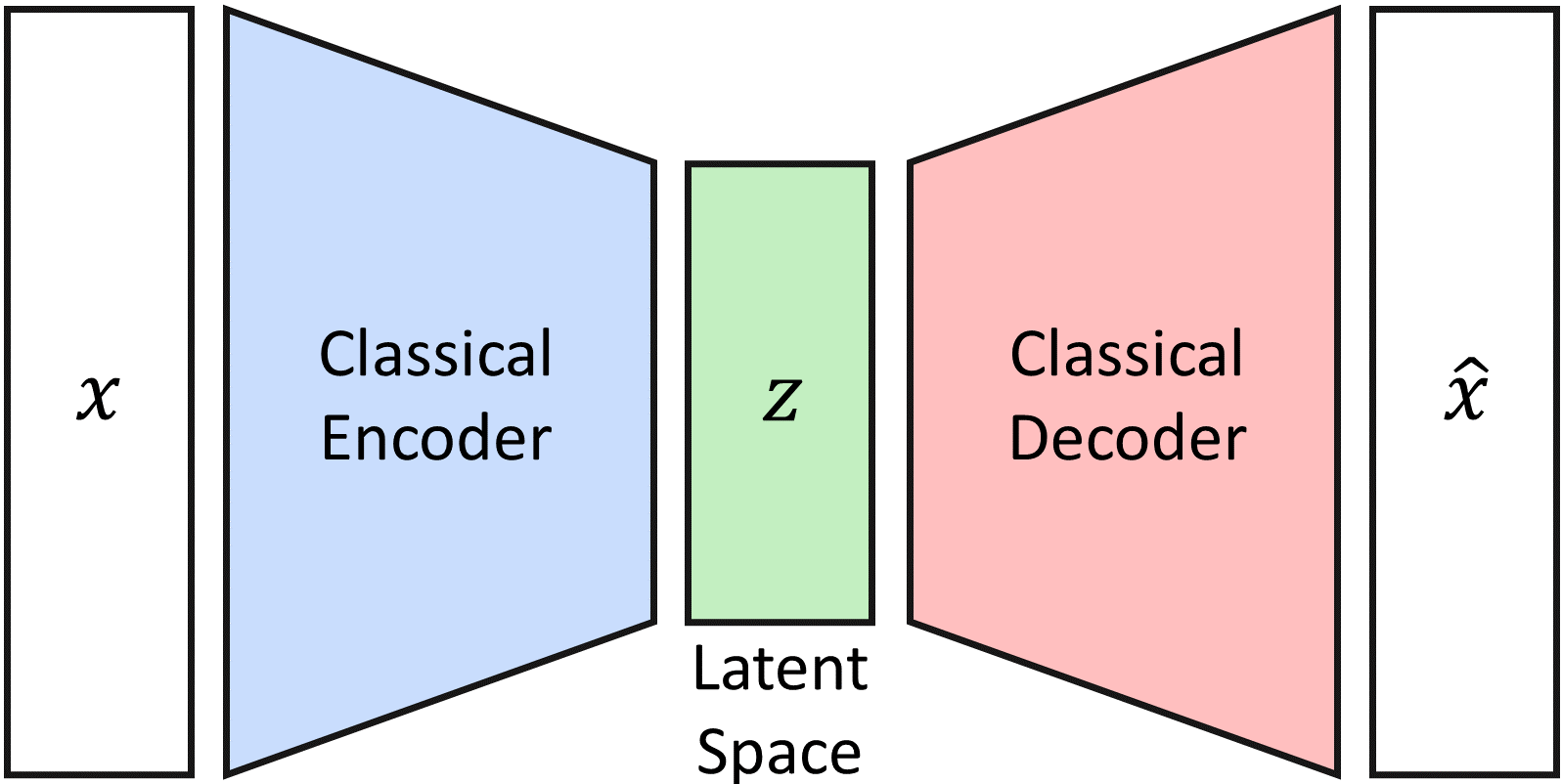
Figure 2: Architecture of classical convolutional autoencoder: The core design of a convolutional autoencoder consists of classical encoder and decoder components, each featuring crucial convolutional layers. These layers play a pivotal role in transforming the input image data $x$ into into a reconstructed representation $\hat{X}$ through the latent space $Z$.

Given an input image data $x$, the process of CCAE is simply defined as follows:

$$\hat{x}=D(Z),Z=E(x),$$ (8)

where the training loss can be defined as follows:

$$L_{AE}=\|x-\hat{x}\|^{2},$$ (9)

and $\|\cdot\|^{2}$ denotes the L2-norm.

4 The proposed method

In this section, we present a comprehensive end-to-end methodology outlining the proposed approach. We first extensively review the proposed technique in its quantum form, after which we meticulously present the quantum circuit using the QAOA method. Finally, we explain how we fine tune and improve the quantum circuit through a training optimization process, focusing on a PSR technique.

4.1 Quantum convolutional autoencoder (QCAE)

In this study, we introduce the QCAE architecture designed for image denoising. Leveraging the CCAE model as its foundation, the QCAE incorporates a QAOA circuit to replace the CCAE’s latent space. The QCAE process involves several key stages: i) initializing the input image data, ii) introducing noise to the input image data to generate a noisy input, iii) encoding the input image data into a quantum state, iv) using a QAOA circuit to manipulate the quantum state, v) measuring the output of the QAOA circuit, and vi) generating denoised input image data through a classical decoder based on the QAOA circuit measurement results [17]. Fig. 3 showcases the QCAE architecture and the steps involved in image denoising. Given a random noise-generating function $S$, the process involves taking an input data $x$ and subjecting it to the influence of $S$ to produce a noisy input image data version represented as $S(x)$. Subsequently, this noisy input $S(x)$ serves as the input for the QCAE. A proficient QCAE model should be capable of efficiently handling noisy images, adeptly processing them to reconstruct the original image, all the while eliminating any undesirable noise.

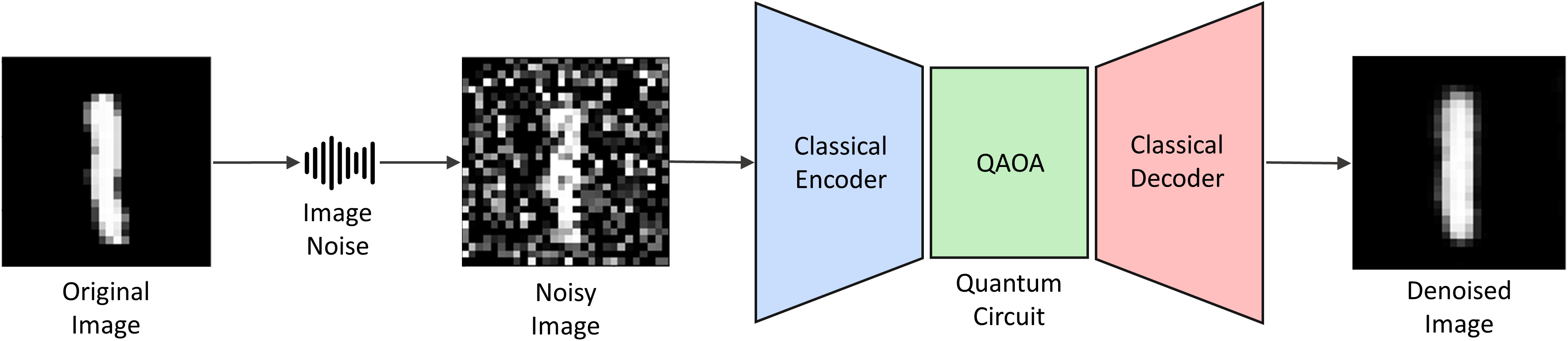
Figure 3: Architecture of quantum convolutional autoencoder, where the classical latent space is replaced with a QAOA circuit to efficiently denoise images.

In the QCAE, the convolutional encoder is responsible for extracting and compressing crucial features from the input image data. Through a carefully designed sequence of convolutional layers, pooling layers, and activation functions, the encoder systematically reduces the dimensionality of the input image data. This process results in the creation of a condensed, low-dimensional latent representation that encapsulates the essential features of the input image [7, 41]. By replacing the classical latent space with the QAOA circuit, one can obtain latent representations that are more effectively optimized for preserving the most crucial features within the input image data [35, 22]. In contrast to the convolutional encoder, the convolutional decoder consists of a series of transposed convolutional layers, upsampling layers, and activation functions. Transposed convolutional layers essentially perform the inverse operation of convolutional layers. These layers augment the spatial dimensions of the feature maps, simultaneously acquiring the ability to reconstruct lost details of the encoded input image data.

4.2 Quantum approximate optimization algorithm (QAOA)

QAOA, originally proposed by Farhi et al. [13], is a heuristic approach specifically designed to tackle the maxcut problem. It belongs to the group of hybrid algorithms and requires, in addition to executing shallow quantum circuits, a classical optimization process to optimize the parameters and improve the quantum circuit itself [16, 8]. The performance of QAOA continually improves with increasing values of $p$, contributing to the achievement of so-called quantum supremacy [14]. As depicted in Fig. 4, the maximum or minimum value of objective function can be obtained by iteratively finding the optimal values for the parameters $\gamma$ and $\beta$. The iterative process for determining the optimal parameters relies on classical optimization methods. In the context of QCAE, the latent space aims to acquire a compressed representation of the input image data, capturing inherent patterns and relationships among the data points. This representation aims to be more compact than the original input data while retaining essential information. Given that the primary objective of QAOA is to identify the optimal solution for a given problem, the QAOA circuit is utilized to discern the quantum information of the input state through the optimal latent representation.

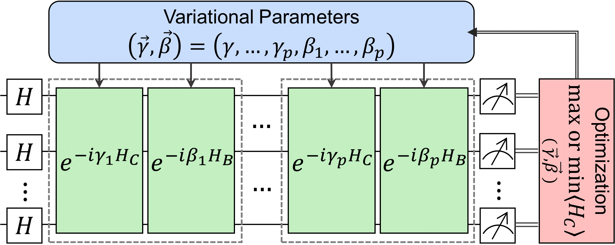
Figure 4: Schematic depicting the quantum approximate optimization algorithm, which integrates a quantum circuit and classical optimization to iteratively optimize variational parameters for enhanced performance.

The algorithm is designed to identify a $n$-bit binary strings $z$, the objective function $f$ is defined as follows:

$$f(z):\{0,1\}^{n}.$$ (10)

We can map $f$ to the Hamiltonian $H_{C}$ as follows:

$$H_{C}|z\rangle=f(z)|z\rangle.$$ (11)

In which the phase operators are defined as follows:

$$U_{C}(\gamma)=e^{-i\gamma H_{C}},$$ (12)

where $\gamma$ is a parameter. The mixing Hamiltonian $H_{B}$ is defined as follows:

$$H_{B}=\sum_{j=1}^{n}\sigma_{j}^{x},$$ (13)

where $\sigma_{j}^{x}$ is the Pauli-X operator. In addition, the mixing operators are defined as follows:

$$U_{B}(\beta)=e^{-i\beta H_{B}},$$ (14)

where $\beta$ is a parameter. We can define the state of the $p$-level QAOA by applying the phase operator and the mixing operator, defined as follows:

$$|\vec{\gamma},\vec{\beta}\rangle=U_{C}(\gamma_{p})U_{B}(\beta_{p})\cdots U_{C}(\gamma_{1})U_{B}(\beta_{1})|s\rangle,$$ (15)

with an integer $p\geq 1$ and $s$ is the initial state, defined according to the superposition principle as follows:

$$|s\rangle=|+\rangle^{\otimes n}=\frac{1}{\sqrt{2^{n}}}\sum_{z}|z\rangle.$$ (16)

The expectation value of $H_{C}$ can be obtained as follows:

$$\langle H_{C}\rangle:=\langle\vec{\gamma},\vec{\beta}|H_{C}|\vec{\gamma},\vec{\beta}\rangle=\langle f\rangle_{(\vec{\gamma},\vec{\beta})},$$ (17)

where $f$ is the expectation value of the objective function.

Here, we then introduce the process of injecting parameter values into rotation gates $R$ parameter placeholders. The training process of the QAOA circuit begins with input image data $x$ and a set of rotation gates $R$ at level $p$. First, the input image data are encoded using a classical encoder $\vec{x}=E(x)$, where $\vec{x}$ is an encoded input image data. Then, this data undergoes additional classical processing through convolutional layers, pooling layers, and is transformed into a linear form of $y$ to the size of $2p$, where $p\geq 1$ is the QAOA circuit level. Classical normalization and optimization techniques are applied to the variable $y$ to fine-tune the parameters, aiming to minimize the objective function (cost function). Fig. 5 illustrates the schematic illustrates the classical encoder in encoding and optimizing input image data for the QAOA circuit at any given $p$ levels.

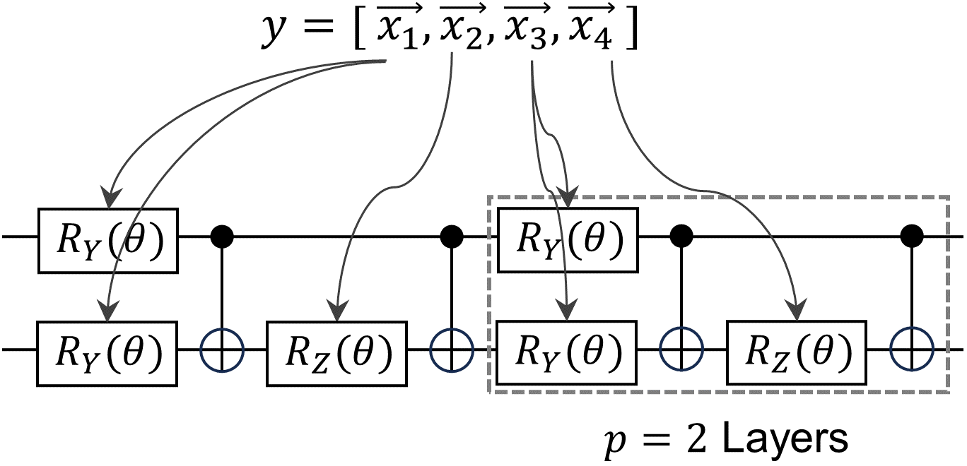
Figure 5: Parameterizing the rotation gates of QAOA circuit with the optimized value of the encoded input image data.

4.3 Parameter-shift rule optimization

In this section, we present a PSR optimization method inspired by [47]. The PSR is a promising approach for evaluating the gradients of QAOA circuits on real quantum machines [10, 49]. Gradients derived from these quantum circuits significantly contribute to the optimization phase of VQAs. In the context of hybrid quantum-classical algorithms, we first construct a quantum circuit and subsequently adjust its parameters to minimize an objective function or cost function [36]. In our proposed method, we compute the gradient of each parameter in the QAOA circuit by per the parameter and determining the difference between two forming a double shift, positive shift and negative shift, on outputs, without modifying the QAOA circuit structure or using any ancilla qubits [47]. Suppose we have an $n$-qubit QAOA circuit which is parameterized by $m$ parameters, $\theta=[\theta_{1},\dotsm,\theta_{i},\dotsm,\theta_{m}]$, the objective function $f(\theta)$ of a quantum circuit can be represented by a circuit function as follows:

$$f(\theta)=\langle\psi|U(\theta_{i})^{\dagger}QU(\theta_{i})|\psi\rangle,$$ (18)

where $\theta_{i}$ is the scalar parameter whose gradient is to be computed and $U(\theta_{i})$ is the unitary gate with a parameter $\theta_{i}$, which is the rotation gate in this paper. For notation simplicity, we will absorb the unitaries before $U(\theta_{i})$ into $\langle\psi|$ and $|\psi\rangle$. Unitaries after $U(\theta_{i})$ and observables are fused into $Q$. The parameterized unitary gates can be basically written in the following form:

$$U(\theta_{i})=e^{-\frac{i}{2}\theta_{i}H},$$ (19)

where $H$ is the Hermitian generator of $U(\theta_{i})$ with only two unique eigenvalues $+1$ and $-1$. In this way, the differences in the gradients of the circuit function $f$ with respect to $\theta_{i}$ are:

$$\begin{array}[]{l}\frac{\partial f(\theta)}{\partial\theta_{i}}=\frac{1}{2}\Bigl{(}f(\theta_{+})-f(\theta_{-})\Bigl{)},\\ \\ \theta_{+}=[\theta_{1},\dotsm,\theta_{i}+\frac{\pi}{2},\dotsm,\theta_{m}],\\ \\ \theta_{-}=[\theta_{1},\dotsm,\theta_{i}-\frac{\pi}{2},\dotsm,\theta_{m}],\end{array}$$ (20)

where $\theta_{+}$ and $\theta_{-}$ are the positive shift and negative shift of $\theta$, respectively. This method precisely computes the gradient with respect to $\theta_{i}$, avoiding any approximation errors. We then apply the softmax function to the objective function obtained from measurements $f(\theta)$ as the predicted probability distribution for positive shift and negative shift. Subsequently, we compute the cross entropy between the predicted probability distribution $pd$ and the target distributed $td$ as the classification loss $L$ as follows:

$$L(\theta)=-td^{T}\cdot softmax(f(\theta))=-\sum_{j=1}^{n}td_{j}\log{pd_{j}},$$ (21)

where

$$pd_{j}=\frac{e^{f_{j}(\theta)}}{\sum_{j=1}^{n}e^{f_{j}(\theta)}}$$ (22)

Then the gradient of the loss function with respect to $\theta_{i}$ can be defined as follows:

$$\frac{\partial L(\theta)}{d\theta_{i}}=\Bigl{(}\frac{\partial L(\theta)}{\partial f(\theta)}\Bigl{)}^{T}\times\;\frac{\partial f(\theta)}{\partial\theta_{i}}$$ (23)

Here $\frac{\partial f(\theta)}{\partial\theta_{i}}$ can be computed on a QAOA circuit utilizing the PSR, while $\frac{\partial L(\theta)}{\partial f(\theta)}$ can be efficiently calculated on classical devices through backpropagation, facilitated by differentiation frameworks, e.g., PyTorch [31] and TensorFlow [1].

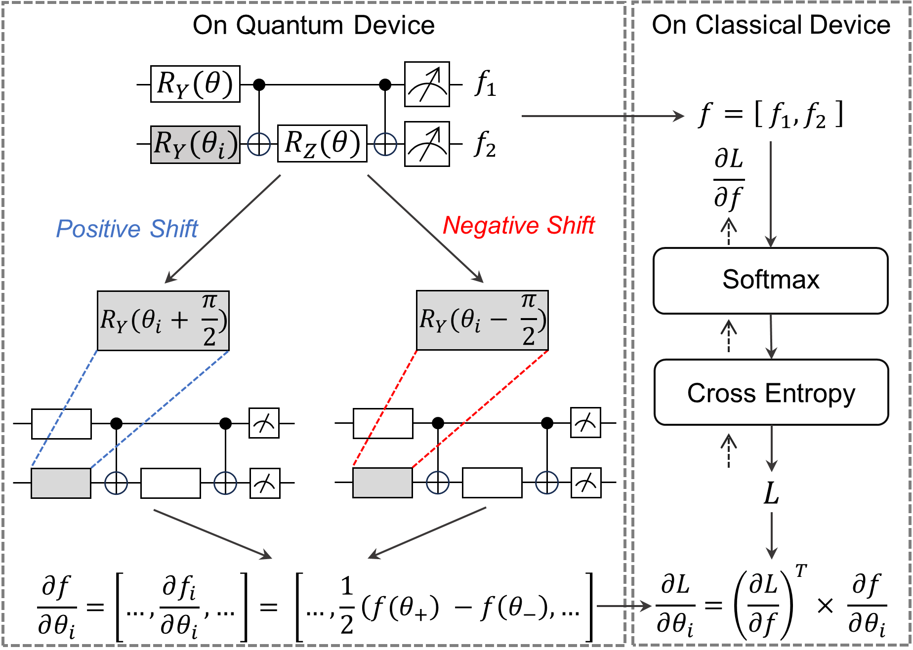
Figure 6: Efficient gradient computation through the technique PSR on a hybrid QAOA circuit.

Fig. 6 visually depicts the procedural steps of the technique PSR. In each iteration, we perform dual shifts of the parameter $\theta_{i}$ by $+\frac{\pi}{2}$ and $-\frac{\pi}{2}$, respectively. After each parameter shift, we execute the shifted QAOA circuit on either a local quantum simulator or a quantum device. Upon obtaining the results from the two shifted circuits, we apply Equation 20 to calculate the upstream gradient. Following the PSR, we then execute the QAOA circuit without any parameter shift and record the measurement results. Subsequently, we apply softmax and cross-entropy functions to the obtained logits, ultimately producing training loss. The backpropagation process is initiated solely from the loss to the logits, generating downstream gradients. Finally, the gradient is computed by taking the dot product between the upstream and downstream gradients, as outlined in Eq. 23, resulting in the final gradient.

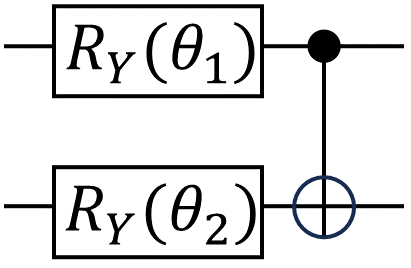
(a) Circuit A

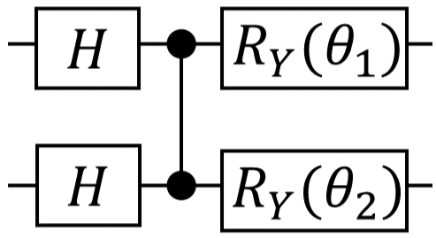
(b) Circuit B

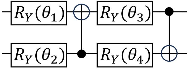
(c) Circuit C

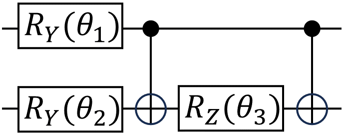
(d) Ours

Figure 7: PQCs utilized in the QAOA circuit. The PQCs (a), (b), and (c) are adapted from [22, 20], whereas (d) is our designed QAOA circuit.

5 Experimental setups

In this section, we outline the datasets used to validate our proposed method and describe the experimental environments for its implementation.

5.1 Datasets

We perform both CCAE and QCAE on the well-known MNIST dataset. This dataset comprises handwritten digits presented as grayscale images. The MNIST dataset comprises 60,000 samples in the training set and 10,000 samples in the testing set, each represented by pixels arranged in a shape of $28\times 28\times 1$. To incorporate noise into the datasets, we used a function that adds random Gaussian noise to the images. The original and noisy images are visualized in Fig. 3. For the MNIST dataset, we selected two specific classes from MNIST (0 and 1). For a fair comparison between CCAE and QCAE, the training datasets comprise the initial 2000 samples.

5.2 Environments

The experiments were conducted using the PyTorch [31] and Qiskit [34] frameworks. The proposed QCAE is tested on both a local quantum simulator equipped with a quantum assembly (QASM) simulation and a 27-qubit IBMQ Mumbai quantum machine. For noisy simulators, we leverage the noise model from IBM Mumbai and inject it into the QASM simulator. For notation simplicity, we designate the QASM simulator as the noiseless simulator, the noisy QASM simulator as the noisy simulator, and the actual quantum machine as the real machine.

For both the CCAE and QCAE, the encoder and decoder architectures comprise three 2D convolutional and 2D transposed convolutional layers, respectively. The only difference lies in the latent space, which is substituted with a QAOA circuit in the case of QCAE. In the CCAE model, the latent space is established through a fully connected layer network, with the classical encoder and decoder employing the LeakyReLU activation function. The training spanned 50 epochs using the Adam optimizer [23] and the mean squared error (MSE) as the loss function. Due to cost and time constraints, we conducted the training in both noiseless and noisy environments, as it required many iterations. To validate the real-world applicability, the testing phase was conducted in a real environment, ensuring the proposed model’s reliability in practical scenarios.

We meticulously execute and perform experiments that encompass a comprehensive array of QAOA circuits. These circuits incorporate diverse configurations of single-qubit and two-qubit gate operations. Our circuit designs were inspired by prior research [22, 20], and their visual representation is illustrated in Fig. 7.

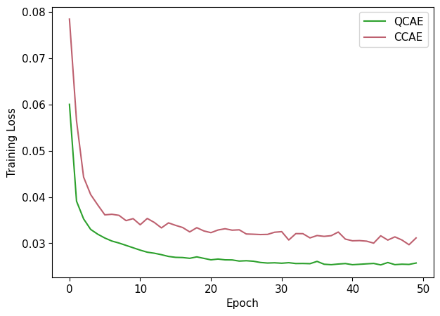
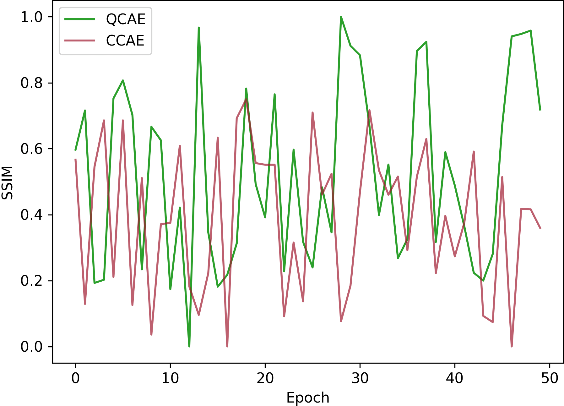
Figure 8: (Left) Comparison of training loss between the CCAE and QCAE models showcases a decrease in loss as the number of epochs increases. (Right) Comparison of SSIM between CCAE and QCAE shows an average SSIM of approximately 0.45 and 0.75, respectively.

6 Experimental results

In this section, we evaluate the performance of our proposed QCAE model on the denoising MNIST dataset. First, we compare the training loss and evaluation of QCAE with CCAE. Second, we analyze the denoising performance of QCAE in noiseless, noisy, and real scenarios. Finally, we conduct ablation studies by varying QAOA circuits and layers to enhance understanding and optimize its overall performance.

6.1 Training of the CCAE and QCAE

In this evaluation, two binary classes were extracted from the MNIST dataset (0 and 1). To gain insights into the distinctions between denoised samples generated by both the CCAE and QCAE models and the original samples, we employ a metric called the structural similarity index measure (SSIM) for analyzing image quality [44], ranging from 0 (worst) to 1 (best). To illustrate the training performance, the left side of Fig. 8 displays the training loss. Our proposed QCAE consistently outperforms CCAE, achieving a lower training loss. The right side of Fig. 8 illustrates the SSIM values over 50 training epochs, demonstrating that QCAE generates denoised images closely resembling and showcasing higher quality compared to those produced by CCAE. This distinction is particularly evident when considering the average of SSIM 0.45 for CCAE and SSIM 0.75 for QCAE. These findings highlight that QCAE consistently delivers robust results when employed for denoising images compared with CCAE.

Fig. 9 depicts original images alongside those with added noise, where high corruption levels render them barely visible to the human eye. The denoising results generated using both QCAE and CCAE models are shown alongside the noisy and original images. Notably, in the third row and middle column, the CCAE struggles to fully denoise or reconstruct the image, highlighting a limitation. Furthermore, CCAE faces challenges in effectively denoising, resulting in denoised results that exhibit a subtle blurring effect when compared to the sharper outcomes achieved by QCAE, with an average SSIM for CCAE at 0.45 and the SSIM for QCAE at 0.75. This performance gap emphasizes the effectiveness of our proposed QCAE, which outperforms CCAE as its classical counterpart.

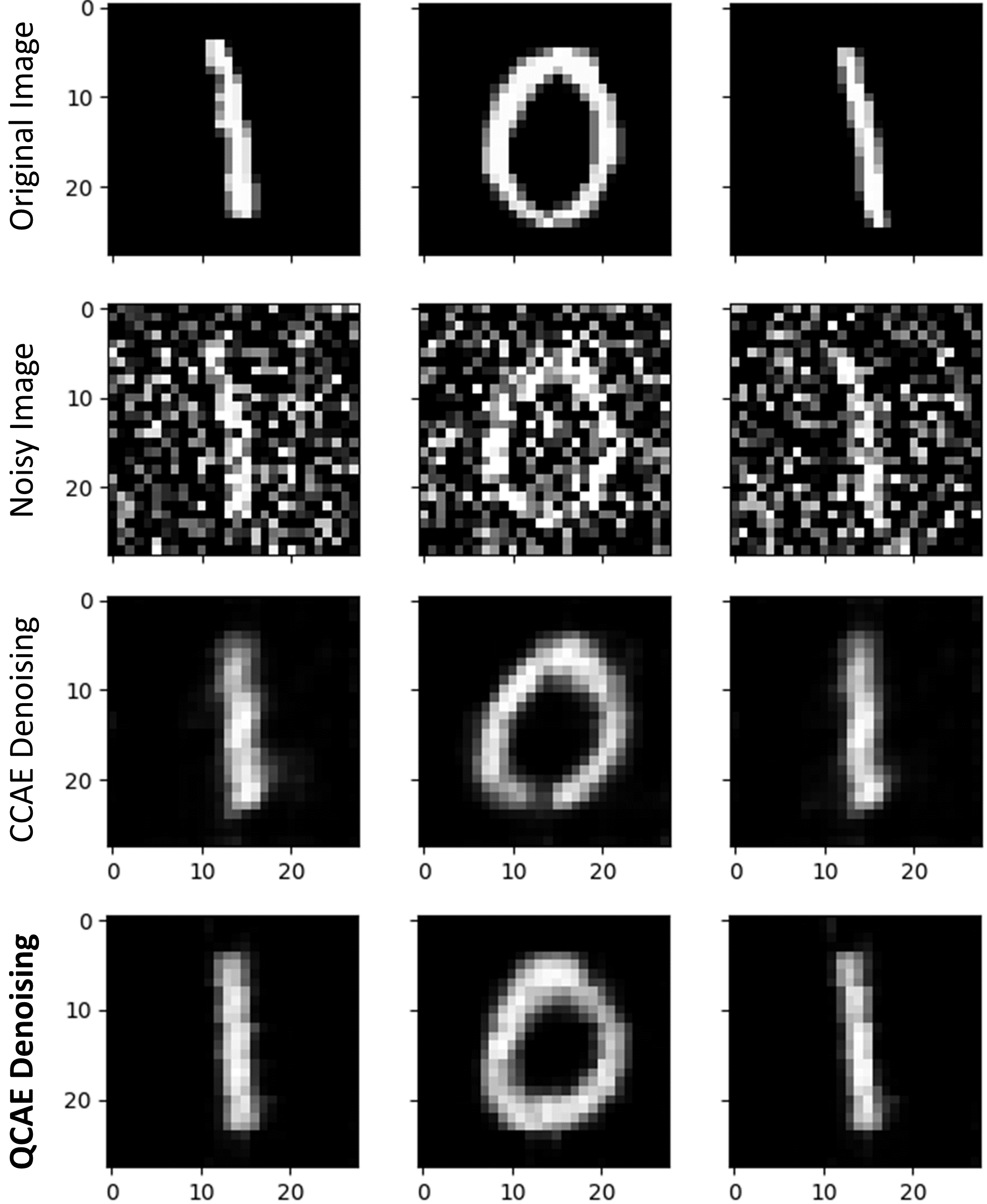
Figure 9: Denoising results on MNIST datasets. The top row displays original images, and the second row shows their noisy counterparts. The third row showcases images denoised with CCAE, and the last row features images denoised using the proposed QCAE method.

6.2 Denoising performance

Here, we conducted denoising of the MNIST images across three distinct scenarios: noiseless, noisy, and real. To effectively demonstrate the performance of the QCAE, we introduced variations in Gaussian noise factors applied to the images because the MNIST does not carry noise. For each scenario, we experiment with the Gaussian noise factor $\sigma=\{0.25,0.5,0.75,1\}$, and choose the optimal combination from 1 out of 12 options based on the reasonable noise factor and highest SSIM for further experiments. The QCAE performance is evaluated for the denoising capability in both quantum simulations and actual machines.

Fig. 10 illustrates the performance of CCAE and specifically QCAE when tested on noisy images with varying noise factors. The findings reveal a notable reduction in SSIM value as the noise factor increases in the image. However, even in the challenging conditions of current noisy and real environments, our proposed QCAE showcases results comparable to noiseless environments. This underscores the robustness of our QCAE, confirming its ability to operate effectively in diverse quantum computer environments. One should take note that the noisy configuration outperforms the real setting, even though both utilize the same IBM machine. This superiority arises from the fact that the noise model incorporates various critical factors, including basic gate error, gate length, decoherence times, and the readout error probability of each qubit. These parameters are calibrated on a daily basis, contributing to a slightly lower level of noise precision compared to the real configuration [24].

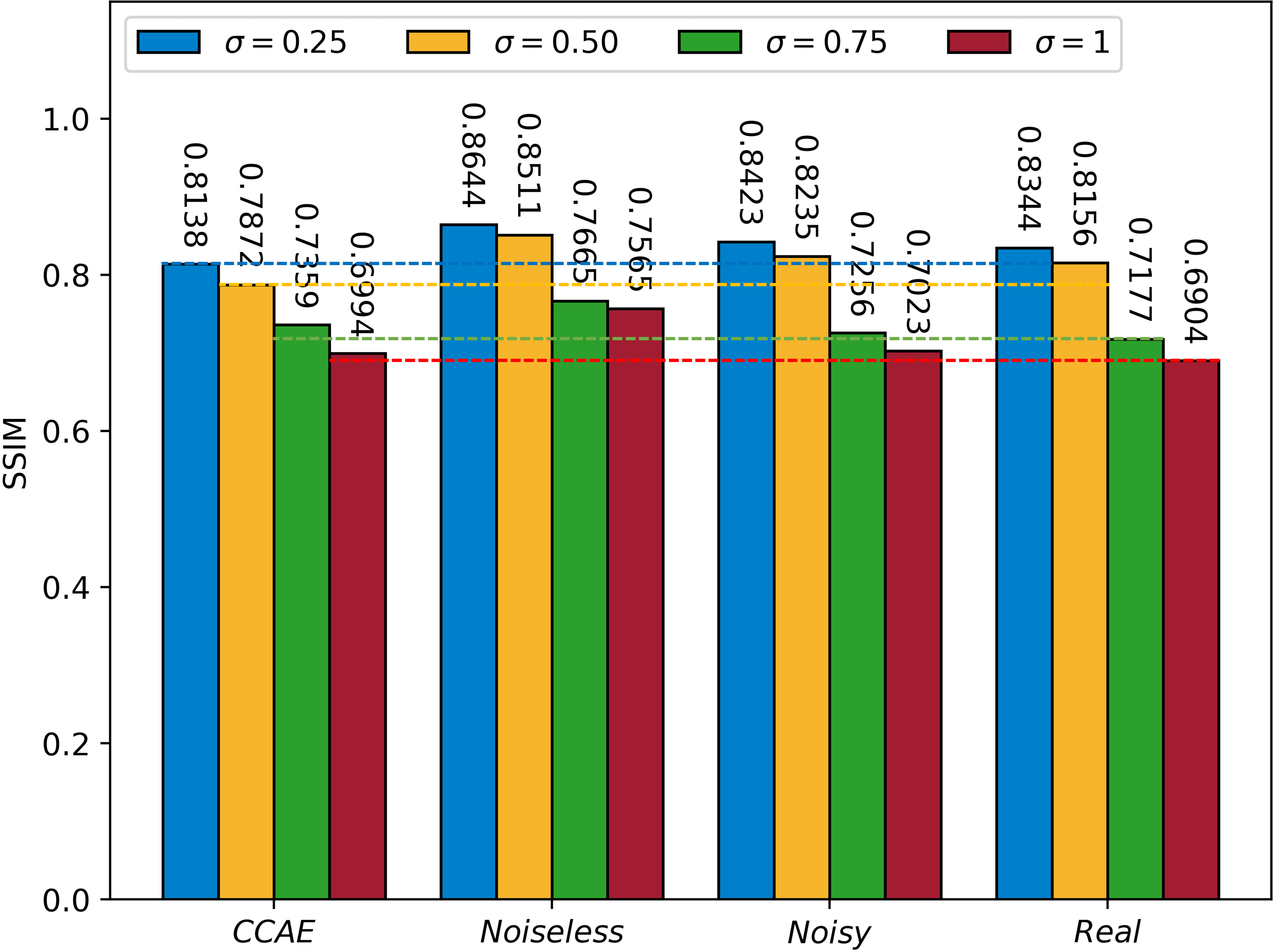
Figure 10: Comparative analysis of the CCAE and specifically QCAE performance under varying conditions, including noiseless, noisy, and real scenarios, with noise factor variations represented by $\sigma=\{0.25,0.5,0.75,1\}$.

To analyze the extent of QCAE denoising capabilities, we utilize it to restructure, denoise, and generate images from a set of noisy inputs with varying noise factors values. Even in the presence of high levels of noise, characterized by a noise factor of $\sigma=1$, images that appear indistinguishable to the human eye are effectively processed by QCAE. The algorithm consistently delivers accurate and visually appealing results, demonstrating its robust performance in handling noisy images. Despite testing in noisy and real quantum machine environments, the image maintains readability and closely resembles the original, although with a slight degradation compared to a noiseless environment. Denoising results, along with variations in Gaussian noise levels and quantum machine environments, are depicted in Fig. 11.

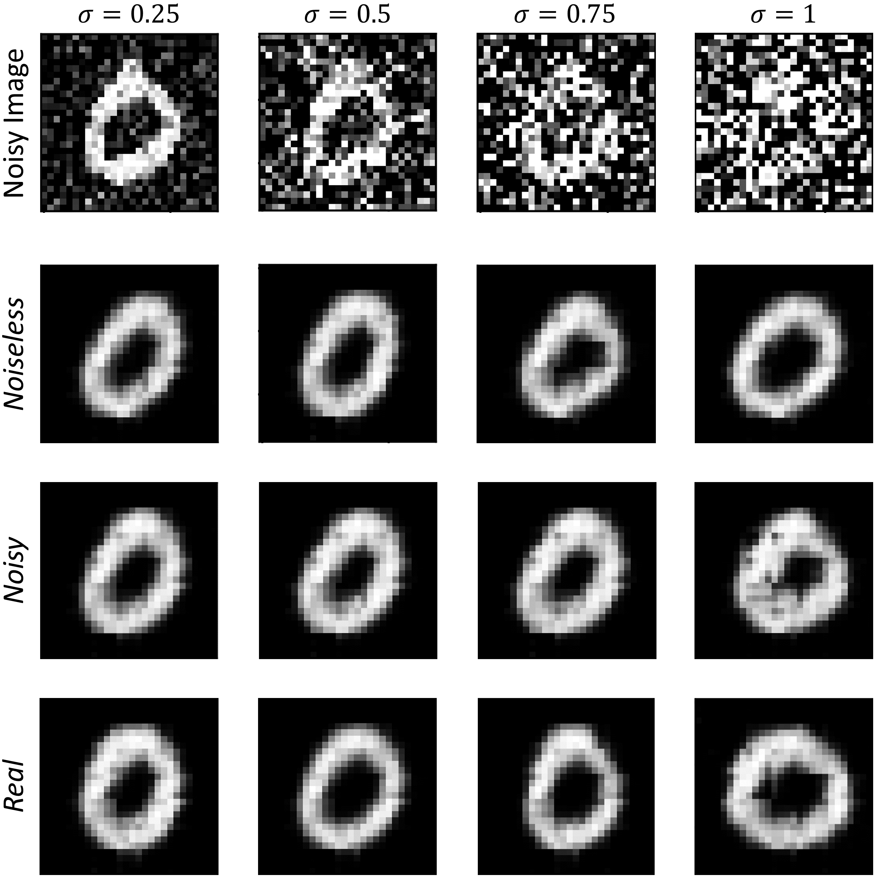
Figure 11: Performance evaluation of QCAE on noisy images across a range of Gaussian noise factors. The top row presents noisy images with $\sigma=\{0.25,0.5,0.75,1\}$. The second row showcases denoised images in a noiseless quantum simulation, whereas the third row showcases denoised images in a noisy quantum simulation. The fourth row displays denoised images with a real quantum machine.

6.3 Comparison of PQCs and PSR optimization

In this study, we conducted experiments employing various quantum circuits sourced from [22, 20], and comparing them to our proposed approach with and without PSR optimization. The experiments were executed with identical configurations, including the number of qubits, epochs, $\sigma=0.5$, optimization using the PSR, a noiseless environment, and the MNIST dataset. In addition, we varied the number of $p$ layers to investigate how circuit depth influences the obtained results. The $p$-value results were validated across a range from 1 to 5 and subsequently categorized into groups corresponding to the respective quantum circuits. Fig. 12 presents the SSIM values obtained from the various circuit types depicted in Fig. 7. Compared to alternative circuits, our proposed approach showcases superior performance across these circuits. Specifically, our proposed QAOA circuit consistently outperforms other circuits, showcasing an average improvement of approximately 25% in the SSIM value.

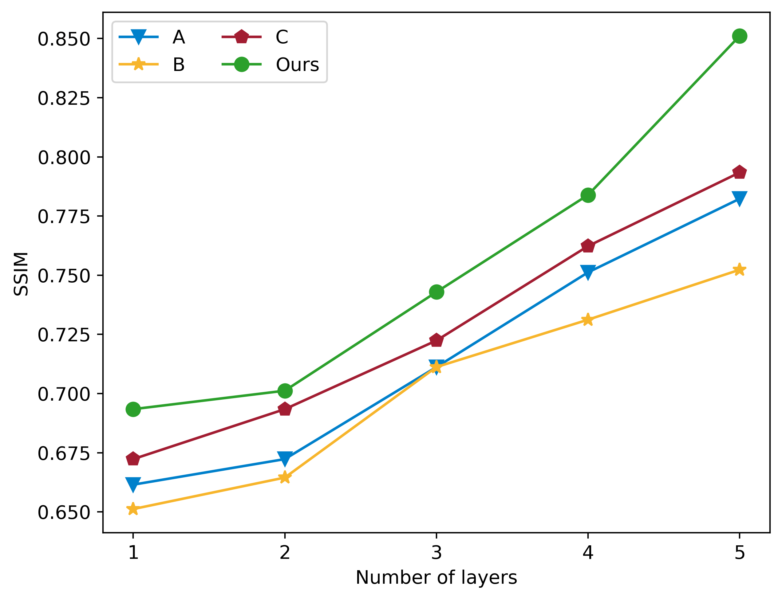
Figure 12: The SSIM value of $p$ ranges from 1 to 5 across all circuits, indicating that better solutions are associated with longer circuit layers.

We also conducted comprehensive experiments on all circuits, both with and without PSR, resulting in a noteworthy reduction in SSIM values when tested without PSR, as shown in Table 1. Remarkably, our proposed circuit demonstrated the ability to draw comparisons with other circuits, even in the absence of PSR. One plausible explanation is that $R_{Z}$ gates can be implemented with greater efficiency compared to other single-qubit rotation operations [25]. As we observed, the circuits exhibit lower and significantly higher SSIM values with and without PSR, respectively. This underscores the significance of incorporating PSR optimization to enhance performance. It is noteworthy that the $p$ value significantly influences the results, underscoring its high impact on the outcomes. However, as the parameter $p$ increases, there is a corresponding growth in the circuit execution time. Additionally, our proposed method requires a minimum of two qubits for the efficient denoising of images. It also illustrates the progressive increase in SSIM values corresponding to the varying number of $p$ layers. As additional layers are added, the QAOA showcases the potential for enhanced approximations towards the optimal solution. Furthermore, it presents the results of experiments conducted on QAOA, both with and without PSR optimization. The findings emphasize the significance of employing this optimization technique to identify a lower-cost function, leading to higher accuracy. Through the utilization of the PSR optimization, there is a notable enhancement in SSIM value. This enhancement showcases an improvement of up to 35% when compared with non-optimized conditions.

Circuits	$p=1$	$p=2$	$p=3$	$p=4$	$p=5$
Without PSR optimization
A	0.4371	0.4398	0.4423	0.4480	0.4512
B	0.4302	0.4357	0.4423	0.4521	0.4553
C	0.4493	0.4523	0.4567	0.4623	0.4663
Ours	0.6503	0.6618	0.7034	0.7235	0.7496
With PSR optimization
A	0.6615	0.6723	0.7112	0.7512	0.7823
B	0.6512	0.6645	0.7112	0.7312	0.7523
C	0.6723	0.6934	0.7224	0.7623	0.7934
Ours	0.6934	0.7012	0.7429	0.7839	0.8511

Table 1: The SSIM value for parameter $p$ varies between 1 and 5 across all circuits, both with and without the utilization of PSR optimization techniques.

7 Conclusion

This study introduced a QCAE model that leverages the power of QAOA to seamlessly substitute for the conventional AE, serving as the latent space. This substitution improves data learning in a higher-dimensional space. We demonstrated the efficiency of our proposed QCAE method through its application to MNIST image denoising. The proposed QCAE method exhibited superior denoising performance, as it achieved lower training loss and increased SSIM, compared to the CCAE method—a finding validated by experimental results—demonstrating its superior capacity to preserve image fidelity. The developed model maintained its superior denoising capabilities when applied to the MNIST dataset. Furthermore, we examined QAOA performance to determine its effectiveness across diverse circuit configurations and layer variations. Finally, we conducted an experiment using PSR optimization to evaluate its impact on QAOA circuit accuracy. This investigation underscores the crucial role of optimization in achieving desirable outcomes. However, we remark that state-of-the-art and out-of-the-box classical algorithms cannot be easily outperformed by current quantum computers and algorithms. The potential future research directions are as follows: First, we aim to evaluate the effectiveness of our proposed approach by conducting tests on real-world practical images and providing evidence to validate its viability. Second, we aim to investigate how different optimization methods affect the performance of our proposed model on the MNIST dataset. Furthermore, given that notice noise in real quantum machines can significantly impact the outcomes of the method, employing noise mitigation techniques is required to address and alleviate these effects.

Code available

The code that supports the findings of this study is openly available in the Github repository: Quantum Autoencoder.

References

- Abadi et al. [2016] Abadi, M., Agarwal, A., Barham, P., Brevdo, E., Chen, Z., Citro, C., Corrado, G.S., Davis, A., Dean, J., Devin, M., et al., 2016. Tensorflow: Large-scale machine learning on heterogeneous distributed systems. arXiv preprint arXiv:1603.04467 .
- Abiodun et al. [2018] Abiodun, O.I., Jantan, A., Omolara, A.E., Dada, K.V., Mohamed, N.A., Arshad, H., 2018. State-of-the-art in artificial neural network applications: A survey. Heliyon 4.
- Baldi [2012] Baldi, P., 2012. Autoencoders, unsupervised learning, and deep architectures, in: Proceedings of ICML workshop on unsupervised and transfer learning, JMLR Workshop and Conference Proceedings. pp. 37–49.
- Benedetti et al. [2019] Benedetti, M., Lloyd, E., Sack, S., Fiorentini, M., 2019. Parameterized quantum circuits as machine learning models. Quantum Science and Technology 4, 043001.
- Bharti et al. [2022] Bharti, K., Cervera-Lierta, A., Kyaw, T.H., Haug, T., Alperin-Lea, S., Anand, A., Degroote, M., Heimonen, H., Kottmann, J.S., Menke, T., et al., 2022. Noisy intermediate-scale quantum algorithms. Reviews of Modern Physics 94, 015004.
- Bouland et al. [2022] Bouland, A., Fefferman, B., Landau, Z., Liu, Y., 2022. Noise and the frontier of quantum supremacy, in: 2021 IEEE 62nd Annual Symposium on Foundations of Computer Science (FOCS), IEEE. pp. 1308–1317.
- Bravo-Prieto [2021] Bravo-Prieto, C., 2021. Quantum autoencoders with enhanced data encoding. Machine Learning: Science and Technology 2, 035028.
- Choi and Kim [2019] Choi, J., Kim, J., 2019. A tutorial on quantum approximate optimization algorithm (qaoa): Fundamentals and applications, in: 2019 International Conference on Information and Communication Technology Convergence (ICTC), IEEE. pp. 138–142.
- Cortese and Braje [2018] Cortese, J.A., Braje, T.M., 2018. Loading classical data into a quantum computer. arXiv preprint arXiv:1803.01958 .
- Crooks [2019] Crooks, G.E., 2019. Gradients of parameterized quantum gates using the parameter-shift rule and gate decomposition. arXiv preprint arXiv:1905.13311 .
- Diwakar and Kumar [2018] Diwakar, M., Kumar, M., 2018. A review on ct image noise and its denoising. Biomedical Signal Processing and Control 42, 73–88.
- Elad et al. [2023] Elad, M., Kawar, B., Vaksman, G., 2023. Image denoising: The deep learning revolution and beyond—a survey paper. SIAM Journal on Imaging Sciences 16, 1594–1654.
- Farhi et al. [2014] Farhi, E., Goldstone, J., Gutmann, S., 2014. A quantum approximate optimization algorithm. arXiv preprint arXiv:1411.4028 .
- Farhi and Harrow [2016] Farhi, E., Harrow, A.W., 2016. Quantum supremacy through the quantum approximate optimization algorithm. arXiv preprint arXiv:1602.07674 .
- Gondara [2016] Gondara, L., 2016. Medical image denoising using convolutional denoising autoencoders, in: 2016 IEEE 16th international conference on data mining workshops (ICDMW), IEEE. pp. 241–246.
- Guerreschi and Matsuura [2019] Guerreschi, G.G., Matsuura, A.Y., 2019. Qaoa for max-cut requires hundreds of qubits for quantum speed-up. Scientific reports 9, 6903.
- Hassan et al. [2024] Hassan, E., Hossain, M.S., Saber, A., Elmougy, S., Ghoneim, A., Muhammad, G., 2024. A quantum convolutional network and resnet (50)-based classification architecture for the mnist medical dataset. Biomedical Signal Processing and Control 87, 105560.
- Huang et al. [2023] Huang, H.L., Xu, X.Y., Guo, C., Tian, G., Wei, S.J., Sun, X., Bao, W.S., Long, G.L., 2023. Near-term quantum computing techniques: Variational quantum algorithms, error mitigation, circuit compilation, benchmarking and classical simulation. Science China Physics, Mechanics & Astronomy 66, 250302.
- Hubregtsen et al. [2021] Hubregtsen, T., Pichlmeier, J., Stecher, P., Bertels, K., 2021. Evaluation of parameterized quantum circuits: on the relation between classification accuracy, expressibility, and entangling capability. Quantum Machine Intelligence 3, 1–19.
- Hur et al. [2022] Hur, T., Kim, L., Park, D.K., 2022. Quantum convolutional neural network for classical data classification. Quantum Machine Intelligence 4, 3.
- Izadi et al. [2023] Izadi, S., Sutton, D., Hamarneh, G., 2023. Image denoising in the deep learning era. Artificial Intelligence Review 56, 5929–5974.
- Kim et al. [2023] Kim, J., Huh, J., Park, D.K., 2023. Classical-to-quantum convolutional neural network transfer learning. Neurocomputing 555, 126643.
- Kingma and Ba [2014] Kingma, D.P., Ba, J., 2014. Adam: A method for stochastic optimization. arXiv preprint arXiv:1412.6980 .
- Liu et al. [2023] Liu, Y., Li, Z., Robertson, A., Fu, X., Song, S.L., 2023. Enabling efficient real-time calibration on cloud quantum machines. IEEE Transactions on Quantum Engineering .
- McKay et al. [2017] McKay, D.C., Wood, C.J., Sheldon, S., Chow, J.M., Gambetta, J.M., 2017. Efficient z gates for quantum computing. Physical Review A 96, 022330.
- Nagavelli et al. [2022] Nagavelli, U., Samanta, D., Chakraborty, P., et al., 2022. Machine learning technology-based heart disease detection models. Journal of Healthcare Engineering 2022.
- Nguyen and Kenyon [2018] Nguyen, N.T., Kenyon, G.T., 2018. Image classification using quantum inference on the d-wave 2x, in: 2018 IEEE International Conference on Rebooting Computing (ICRC), IEEE. pp. 1–7.
- Nielsen and Chuang [2010] Nielsen, M.A., Chuang, I.L., 2010. Quantum computation and quantum information. Cambridge university press.
- Orduz et al. [2021] Orduz, J., Rivas, P., Baker, E., 2021. Quantum circuits for quantum convolutions: A quantum convolutional autoencoder. Transactions on Computational Science and Computational Intelligence. Springer .
- Ovalle-Magallanes et al. [2023] Ovalle-Magallanes, E., Alvarado-Carrillo, D.E., Avina-Cervantes, J.G., Cruz-Aceves, I., Ruiz-Pinales, J., 2023. Quantum angle encoding with learnable rotation applied to quantum–classical convolutional neural networks. Applied Soft Computing 141, 110307.
- Paszke et al. [2019] Paszke, A., Gross, S., Massa, F., Lerer, A., Bradbury, J., Chanan, G., Killeen, T., Lin, Z., Gimelshein, N., Antiga, L., et al., 2019. Pytorch: An imperative style, high-performance deep learning library. Advances in neural information processing systems 32.
- Paul et al. [2022] Paul, A., Kundu, A., Chaki, N., Dutta, D., Jha, C., 2022. Wavelet enabled convolutional autoencoder based deep neural network for hyperspectral image denoising. Multimedia tools and applications , 1–27.
- Paul and Sabeenian [2022] Paul, E., Sabeenian, R., 2022. Modified convolutional neural network with pseudo-cnn for removing nonlinear noise in digital images. Displays 74, 102258.
- Qiskit contributors [2023] Qiskit contributors, 2023. Qiskit: An open-source framework for quantum computing.
- Rivas et al. [2021] Rivas, P., Zhao, L., Orduz, J., 2021. Hybrid quantum variational autoencoders for representation learning, in: 2021 International Conference on Computational Science and Computational Intelligence (CSCI), IEEE. pp. 52–57.
- Romero et al. [2017] Romero, J., Olson, J.P., Aspuru-Guzik, A., 2017. Quantum autoencoders for efficient compression of quantum data. Quantum Science and Technology 2, 045001.
- Sagha et al. [2017] Sagha, H., Cummins, N., Schuller, B., 2017. Stacked denoising autoencoders for sentiment analysis: a review. Wiley Interdisciplinary Reviews: Data Mining and Knowledge Discovery 7, e1212.
- Sagheer and George [2020] Sagheer, S.V.M., George, S.N., 2020. A review on medical image denoising algorithms. Biomedical signal processing and control 61, 102036.
- Schneider et al. [2022] Schneider, S., Antensteiner, D., Soukup, D., Scheutz, M., 2022. Autoencoders-a comparative analysis in the realm of anomaly detection, in: Proceedings of the IEEE/CVF Conference on Computer Vision and Pattern Recognition, pp. 1986–1992.
- National Academies of Sciences et al. [2019] National Academies of Sciences, E., Medicine, et al., 2019. Quantum computing: progress and prospects .
- Shiba et al. [2019] Shiba, K., Sakamoto, K., Yamaguchi, K., Malla, D.B., Sogabe, T., 2019. Convolution filter embedded quantum gate autoencoder. arXiv preprint arXiv:1906.01196 .
- Sleeman et al. [2020] Sleeman, J., Dorband, J., Halem, M., 2020. A hybrid quantum enabled rbm advantage: convolutional autoencoders for quantum image compression and generative learning, in: Quantum information science, sensing, and computation XII, SPIE. pp. 23–38.
- Stein et al. [2021] Stein, S.A., L’Abbate, R., Mu, W., Liu, Y., Baheri, B., Mao, Y., Qiang, G., Li, A., Fang, B., 2021. A hybrid system for learning classical data in quantum states, in: 2021 IEEE International Performance, Computing, and Communications Conference (IPCCC), IEEE. pp. 1–7.
- Tanchenko [2014] Tanchenko, A., 2014. Visual-psnr measure of image quality. Journal of Visual Communication and Image Representation 25, 874–878.
- Venkataraman [2022] Venkataraman, P., 2022. Image denoising using convolutional autoencoder. arXiv preprint arXiv:2207.11771 .
- Wang et al. [2022a] Wang, F., Xu, Z., Ni, W., Chen, J., Pan, Z., et al., 2022a. An adaptive learning image denoising algorithm based on eigenvalue extraction and the gan model. Computational Intelligence and Neuroscience 2022.
- Wang et al. [2022b] Wang, H., Li, Z., Gu, J., Ding, Y., Pan, D.Z., Han, S., 2022b. Qoc: quantum on-chip training with parameter shift and gradient pruning, in: Proceedings of the 59th ACM/IEEE Design Automation Conference, pp. 655–660.
- Wang et al. [2022c] Wang, Y., Wang, Y., Chen, C., Jiang, R., Huang, W., 2022c. Development of variational quantum deep neural networks for image recognition. Neurocomputing 501, 566–582.
- Wierichs et al. [2022] Wierichs, D., Izaac, J., Wang, C., Lin, C.Y.Y., 2022. General parameter-shift rules for quantum gradients. Quantum 6, 677.
- Yan et al. [2023] Yan, S., Shao, H., Xiao, Y., Liu, B., Wan, J., 2023. Hybrid robust convolutional autoencoder for unsupervised anomaly detection of machine tools under noises. Robotics and Computer-Integrated Manufacturing 79, 102441.