A Hamilton-Jacobi-Bellman Approach to Ellipsoidal Approximations of Reachable Sets for Linear Time-Varying Systems

Abstract

Reachable sets for a dynamical system describe collections of system states that can be reached in finite time, subject to system dynamics. They can be used to guarantee goal satisfaction in controller design or to verify that unsafe regions will be avoided. However, general-purpose methods for computing these sets suffer from the curse of dimensionality, which typically prohibits their use for systems with more than a small number of states, even if they are linear. In this paper, we demonstrate that viscosity supersolutions and subsolutions of a Hamilton-Jacobi-Bellman equation can be used to generate, respectively, under-approximating and over-approximating reachable sets for time-varying nonlinear systems. Based on this observation, we derive dynamics for a union and intersection of ellipsoidal sets that, respectively, under-approximate and over-approximate the reachable set for linear time-varying systems subject to an ellipsoidal input constraint and an ellipsoidal terminal (or initial) set. We demonstrate that the dynamics for these ellipsoids can be selected to ensure that their boundaries coincide with the boundary of the exact reachable set along a solution of the system. The ellipsoidal sets can be generated with polynomial computational complexity in the number of states, making our approximation scheme computationally tractable for continuous-time linear time-varying systems of relatively high dimension.
Keywords: Reachability analysis, Hamilton-Jacobi equations, linear systems, optimal control

1 Introduction

The development of self-driving cars, the use of collaborative robots in industrial settings, and the deployment of drones in disaster responses are exemplars of society’s ever-increasing reliance and integration of autonomous systems in day-to-day life. How can we be certain that these systems will complete their intended task and is it possible for them to behave unsafely? It is such concerns that give impetus to research into methods of verifying the safety and reliability of these systems, and reachable sets lend themselves well to this task. When computed backwards in time, these sets describe all initial states for which there exists a constraint admissible control that leads the system to a set $\mathcal{X}$ at a terminal time $T$ (see Fig. 1). These sets can be used to design controllers with rigorous guarantees of goal satisfaction, which have been previously deployed for maneuvering autonomous cars [1] and lane merging of unmanned aerial vehicles [2]. When computed forwards in time, we obtain the set of states that can be reached using an admissible control starting from $\mathcal{X}$ at some initial time $t$. This information can be used to verify that an autonomous system will not enter an unsafe region due to an adversarial input, which is useful in developing collision avoidance control strategies [3] or guaranteeing the existence of collision free paths [4].

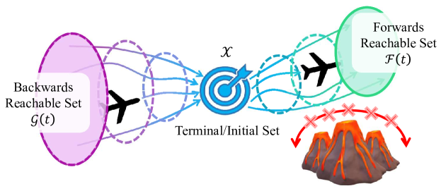
Figure 1: Diagram depicting the backwards reachable set $\mathcal{G}(t)$ and the forwards reachable set $\mathcal{F}(t)$, which enclose all admissible trajectories heading to or away from the set $\mathcal{X}$.

Hamilton-Jacobi (HJ) reachability frames the computation of reachable sets as an optimal control problem. It is a versatile formulation that allows for the direct treatment of nonlinear systems [5], two-player game settings [6], and handling of state constraints [7]. To perform reachability analysis, publicly available toolboxes, such as [8], provide a means of numerically solving HJ equations over a grid in state-space. However, these approaches exhibit computational times that scale exponentially with the number of system states, rendering such schemes computationally intractable for many engineering applications. Consequently, a large body of research in this field focuses on efficient ways to compute or approximate reachable sets.

When dealing with linear systems, a range of approximation schemes are available. In a discrete-time setting, where the terminal or initial set is a polytope and the input set is also a polytope, the reachable sets have an exact polytopic representation [9, Chap. 10]. However, the number of linear inequalities required to represent these polytopes grows with each time step, leading to issues with storage capacity and memory requirements. The use of zonotopes in [10] and [11] can mitigate some of these issues due to their highly efficient set operations. Ellipsoidal approximation schemes have also garnered popularity in both discrete-time [12] and continuous-time settings [13] as ellipsoids can be represented with a fixed number of parameters. Generalisations of these geometries have also been studied, such as ellipsotopes [14], which subsume both ellipsoids and zonotopes, and in characterisations based on support functions [15]. The linchpin in the aforementioned research is that approximations of the Minkowski sum can be used to develop under- and over-approximation (subset and superset) guarantees for reachability of linear systems.

When it comes to nonlinear systems, linearisation-based techniques such as the Taylor series approximation [16] or Koopman operator linearisation [17], are common methods for leveraging existing algorithms for linear systems. Otherwise, efficient algorithms may be available, for instance, when the system can be decomposed into subsystems [18] or when a mixed monotone embedding exists [19]. Other approximation methods include implicit storage of the sets using classification-based control laws [20], neural network approximations [21], and boundary approximations [22].

In this paper, we demonstrate that viscosity supersolutions and subsolutions of a Hamilton-Jacobi-Bellman partial differential equation (HJB PDE) can be used to produce under- and over-approximations of reachable sets for time-varying nonlinear systems in continuous-time. This observation is then used to develop under- and over-approximation schemes for linear time-varying (LTV) systems with ellipsoidal input constraints and ellipsoidal terminal/initial sets. We focus on a single player setting, which is a special case of the problem considered in [6]. Our approach employs the union and intersection of a family of ellipsoids to approximate reachable sets. These results extend on the authors’ prior work in [23], whereby classical supersolutions and subsolutions were used to develop ellipsoidal approximation schemes for linear time-invariant systems. By using viscosity solutions as opposed to classical solutions, approximating sets with non-smooth boundaries can be considered, for example, when the approximating set is constructed via the union or intersection of sets with smooth boundaries. A similar idea is utilised in [24], albeit with classical supersolutions and subsolutions under a different set of assumptions for bilinear systems.

A key difference in our procedure, compared to the vast majority of literature for linear systems, is that we do not rely on approximations of set operations. In particular, we need not deviate from the HJB framework used in nonlinear reachability analysis, thereby allowing for a unified treatment of both nonlinear and linear systems. Moreover, the approximating reachable sets developed through supersolutions and subsolutions of the HJB PDE possess the same desirable characteristics as existing approximation schemes. For instance, the proposed under- and over-approximating collection of ellipsoids, generated via integration of a set of ODEs, are also, respectively, under- and over-approximating for all intermediate times. This corresponds to the recurrence relation discussed in [25], which is inherently built into our approach. The dynamics of each ellipsoid can be chosen to guarantee that their boundaries coincide with the exact reachable set along a solution of the system, which recovers the tightness property discussed in [26]. Additionally, the approximating reachable sets inherit the recursive feasibility and recursive infeasibility properties of the exact reachable set. Specifically, if the system lies within the under-approximating set at a given time, then there exists a constraint admissible control that leads the system to the under-approximating set for any future time. Analogously, if the system is initialised outside the over-approximating set, then it is impossible for the system to be driven into the over-approximating set for any future time. Thus, these approximating sets preserve the intended purpose of reachable sets in control applications.

The remainder of this paper is organised as follows. In Section 2, we review the necessary preliminaries on HJB reachability analysis. In Section 3, we generate approximate reachability results for time-varying nonlinear systems. We then specialise to LTV systems in Section 4, leading to the development of ellipsoidal approximation schemes for LTV systems. A numerical example is considered in Section 5 to illustrate our approximation schemes.

Notation

• Let ${\mathbb{N}}\doteq\{1,2,\ldots\}$ denote the set of natural numbers and let ${\mathbb{R}}_{>0}$ denote the set of positive real numbers.

• We use $\langle\cdot,\cdot\rangle$ to denote the Euclidean inner product and $\left\lVert\cdot\right\rVert_{2}\doteq\left\langle\cdot,\cdot\right\rangle^{\frac{1}{2}}$ to denote the corresponding norm.

• We use $\left\lVert\cdot\right\rVert$ to denote any norm of a vector.

• We use ${\mathscr{A}}^{c},\text{int}\left({\mathscr{A}}\right),\text{cl}\left({\mathscr{A}}\right)$, and $\partial{\mathscr{A}}$ to denote the complement, interior, closure, and boundary of a set ${\mathscr{A}}$, respectively.

• We say that set ${\mathscr{A}}$ under-approximates (resp. over-approximates) set ${\mathscr{B}}$ if ${\mathscr{A}}$ is a non-strict subset (resp. superset) of ${\mathscr{B}}$, i.e., ${\mathscr{A}}\subseteq{\mathscr{B}}$ (resp. ${\mathscr{A}}\supseteq{\mathscr{B}}$).

• The space of $k$-times continuously differentiable functions from $\Omega$ to ${\mathscr{A}}$ is denoted by ${\mathscr{C}}^{k}(\Omega;\,{\mathscr{A}})$ with ${\mathscr{C}}(\Omega;\,{\mathscr{A}})\doteq{\mathscr{C}}^{0}(\Omega;\,{\mathscr{A}})$ denoting the space of continuous functions from $\Omega$ to ${\mathscr{A}}$. Unless stated otherwise, if ${\mathscr{A}}$ is a matrix space, continuity is defined with respect to the induced Euclidean norm.

• The pre-image of a set ${\mathscr{A}}_{0}\subset{\mathscr{A}}$ under $v:\Omega\rightarrow{\mathscr{A}}$ is denoted by $v^{-1}\left({\mathscr{A}}_{0}\right)\doteq\{\omega\in\Omega\,|\,v(\omega)\in{\mathscr{A}}_{0}\}$.

• An open ball of radius $R>0$ centred at $x_{0}\in{\mathbb{R}}^{n}$ is denoted by ${\mathbb{B}}_{R}(x_{0})\doteq\{x\in{\mathbb{R}}^{n}\,|\,\left\lVert x-x_{0}\right\rVert<R\}$.

• We use $A\succ 0$ (resp. $A\succeq 0$) to say that a matrix $A\in{\mathbb{R}}^{n\times n}$ is positive definite (resp. semi-definite).

• The set of symmetric, symmetric positive definite, and symmetric positive semi-definite matrices in ${\mathbb{R}}^{n\times n}$ is denoted by $\mathbb{S}^{n}$, $\mathbb{S}^{n}_{>0}$, and $\mathbb{S}^{n}_{\geq 0}$, respectively.

• The set of orthogonal matrices in ${\mathbb{R}}^{n\times n}$ is denoted by $\mathbb{O}^{n}$.

• We use $\mathbb{I}$ to denote the identity matrix whose size can be inferred from context.

• We denote by $\underline{\Lambda}(A)$ the smallest eigenvalue of $A\in\mathbb{S}^{n}$.

• Finally, the square root of $A\in\mathbb{S}^{n}_{\geq 0}$ is a square matrix denoted by $A^{\frac{1}{2}}\in\mathbb{S}^{n}_{\geq 0}$ and satisfies $A=A^{\frac{1}{2}}A^{\frac{1}{2}}$.

2 Background Theory

2.1 Hamilton-Jacobi-Bellman Reachability Analysis

We begin by reviewing the problem set up for HJB reachability. Fix $T\geq t\geq 0$, $x\in{\mathbb{R}}^{n}$, and consider a finite dimensional time-varying nonlinear system evolving in continuous time, with trajectories satisfying the Cauchy problem

$$\begin{split}\dot{x}(s)&=f(s,x(s),u(s)),\quad\text{a.e }s\in(t,T),\\ x(t)&=x,\end{split}$$ (1)

where $x(s)\in\mathbb{R}^{n}$ is the state and $u(s)\in{\mathbb{U}}$ is the input, both at time $s$, with ${\mathbb{U}}\subset\mathbb{R}^{m}$ assumed to be compact and non-empty. The control input is selected such that $u\in{\mathscr{U}}[t,T]$, where

$${\mathscr{U}}[t,T]\doteq\left\{u:[t,T]\rightarrow\mathbb{U}\;|\;u\text{ measurable}\right\}.$$

Additionally, we assume the following for $f$ throughout.

Assumption 1.

The function $f:[0,T]\times\mathbb{R}^{n}\times\mathbb{U}\rightarrow\mathbb{R}^{n}$ satisfies

1. $f\in{\mathscr{C}}\left([0,T]\times\mathbb{R}^{n}\times\mathbb{U};\,\mathbb{R}^{n}\right)$; and

2. $f$ is Lipschitz continuous in $x$, uniformly in $s$ and $u$, that is, there exists a Lipschitz constant $L_{f}\geq 0$ such that $\left\lVert f(s,x,u)-f(s,y,u)\right\rVert\leq L_{f}\left\lVert x-y\right\rVert$ for all $(s,x,y,u)\in[0,T]\times{\mathbb{R}}^{n}\times{\mathbb{R}}^{n}\times{\mathbb{U}}$.

Under Assumption 1, the dynamics in (1) admit a unique and continuous solution for any fixed control $u\in{\mathscr{U}}[t,T]$ (see [27, Theorem 3.2, p.93]). We denote these solutions at time $s\in[t,T]$ by $\varphi(s;t,x,u)$. In order to consider closed terminal/initial sets, an additional assumption for compactness of solutions of (1) is required, see for example [28, Theorem 7.1.6 and Remarks 7.1.7-7.1.8, pp.190-191].

Assumption 2.

For any $x\in{\mathbb{R}}^{n}$ and $s\in[0,T]$, the set $f(s,x,{\mathbb{U}})\doteq\{f(s,x,u)\,|\,u\in{\mathbb{U}}\}$ is convex.

Remark 1.

If (1) is control affine, that is, $f:[0,T]\times{\mathbb{R}}^{n}\times{\mathbb{U}}\rightarrow{\mathbb{R}}$ can be decomposed as $f(s,x,u)=f_{1}(s,x)+f_{2}(s,x)u$ and ${\mathbb{U}}$ is convex then Assumption 2 is satisfied.

The backwards reachable set for (1), which we denote by $\mathcal{G}(t)$, is defined as the set states at time $t\leq T$ for which there exists a control $u\in{\mathscr{U}}[t,T]$ that leads the system to a set $\mathcal{X}$ at the terminal time $T$. We assume that $\mathcal{X}$ can be described by the zero sublevel set of a real-valued function, in particular,

$$\mathcal{X}\doteq\left\{x\in\mathbb{R}^{n}\,|\,g(x)\leq 0\right\},$$ (2)

where $g\in{\mathscr{C}}({\mathbb{R}}^{n};\,{\mathbb{R}})$. We define $\mathcal{G}(t)$ more precisely below.

Definition 1.

The backwards reachable set of (1) at time $t\in[0,T]$ is defined by

$$\mathcal{G}(t)\doteq\left\{x\in\mathbb{R}^{n}\,|\,\exists\,u\in{\mathscr{U}}[t,T]\text{ s.t. }\varphi(T;t,x,u)\in\mathcal{X}\right\}.$$ (3)

HJB reachability characterises $\mathcal{G}(t)$ as the zero sublevel set of a value function $v:[0,T]\times\mathbb{R}^{n}\rightarrow{\mathbb{R}}$ corresponding to the Mayer optimal control problem given by

$$v(t,x)\doteq\inf_{u\in{\mathscr{U}}[t,T]}g\left(\varphi(T;t,x,u)\right),$$ (4)

which in turn is the viscosity solution to a HJB PDE [28, Theorem 7.2.4, p.194]. Before we state this result, let us attach to (1) a Hamiltonian $H:[0,T]\times\mathbb{R}^{n}\times\mathbb{R}^{n}\rightarrow\mathbb{R}$ given by

$$H(t,x,p)\doteq\max_{u\in{\mathbb{U}}}\left\langle-p,f(t,x,u)\right\rangle.$$ (5)

We recall the disturbance-free case of [6, Lemma 8] below.

Theorem 1.

Let $f:[0,T]\times{\mathbb{R}}^{n}\times{\mathbb{U}}\rightarrow{\mathbb{R}}$ satisfy Assumptions 1 and 2. Consider the HJB PDE given by

$$\begin{split}-v_{t}+H(t,x,\nabla v)&=0,\quad\forall(t,x)\in(0,T)\times\mathbb{R}^{n},\\ v(T,x)&=g(x),\quad\forall x\in\mathbb{R}^{n},\end{split}$$ (6)

where $g\in{\mathscr{C}}\left({\mathbb{R}}^{n};\,{\mathbb{R}}\right)$ defines the terminal set $\mathcal{X}$ in (2), and the Hamiltonian $H$ is defined as in (5). Then, (6) admits the unique viscosity solution $v\in{\mathscr{C}}([0,T]\times\mathbb{R}^{n}\,;\mathbb{R})$ given by (4) and the backwards reachable set for (1) at time $t\in[0,T]$ is

$$\mathcal{G}(t)=\left\{x\in\mathbb{R}^{n}\;|\;v(t,x)\leq 0\right\}.$$

Note that uniqueness of solutions of (6) follows from [29, Theorem 3.17, p.159] with the extension to the non-autonomous setting following from [29, Remark 3.10, pp.154-155] and [29, Exercises 3.6-3.7, pp.182-183].

An analogous set to the backwards reachable set $\mathcal{G}(t)$ is the forwards reachable set $\mathcal{F}(t)$, which characterises all states that can be reached by time $T\geq t$ from the set $\mathcal{X}$ starting at time $t$ under the influence of a constraint admissible control. The forwards reachable set is more precisely defined below.

Definition 2.

The forwards reachable set of (1) at time $t\in[0,T]$ is defined as the set

$$\mathcal{F}(t)\doteq\{\varphi(T;t,x,u)\in\mathbb{R}^{n}\,|\,u\in{\mathscr{U}}[t,T]\text{ and }x\in\mathcal{X}\}.$$ (7)

It turns out that the forwards reachable set is exactly the backwards reachable set of the time-reversed system given by

$$\begin{split}\dot{x}(s)&=-f(T+t-s,x(s),u(s)),\quad\text{a.e }s\in(t,T),\\ x(t)&=x,\end{split}$$ (8)

where $f$ is given in (1). The following theorem states this relationship. We omit the proof for brevity, but the autonomous case appears in Proposition 6 of [30] and similar arguments to Theorem 4 of [22] can be used to demonstrate this result.

Lemma 1.

Let $\mathcal{G}_{-}(t)$ denote the backwards reachable set defined in (3) for the time-reversed system in (8) and let $\mathcal{F}(t)$ denote the forwards reachable set as defined in (7). Then, $\mathcal{F}(t)=\mathcal{G}_{-}(t)$ for all $t\in[0,T]$.

The remainder of this paper will focus on the backwards reachable set, noting that analogous results for forwards reachability can be produced via Lemma 1.

2.2 Viscosity Solutions of HJB Equations

To handle approximating reachable sets that are characterised by potentially non-smooth manifolds, we will need to consider supersolutions and subsolutions of (6) in the viscosity sense. Accordingly, we recall the necessary background and definitions associated with viscosity solutions, which we adapt from [31]. Consider the HJB equation given by

$$-v_{t}+H(t,x,\nabla v)=0,\quad\forall(t,x)\in\Omega,$$ (9)

where $T>0$ is a priori fixed, $\Omega\subseteq(0,T)\times\mathbb{R}^{n}$ is an open set, and $H:\Omega\times\mathbb{R}^{n}\rightarrow\mathbb{R}$ is a continuous function (which corresponds to (5) in our work).

Definition 3.

A function $v\in{\mathscr{C}}\left([0,T]\times{\mathbb{R}}^{n};\,\mathbb{R}\right)$ is a continuous viscosity supersolution (resp. subsolution) of (9) if, for every $\xi\in{\mathscr{C}}^{1}\left(\Omega;\,\mathbb{R}\right)$ that results in $v-\xi$ attaining a local minimum (resp. local maximum) at $(t_{0},x_{0})\in\Omega$,

$$-\xi_{t}(t_{0},x_{0})+H(t_{0},x_{0},\nabla\xi(t_{0},x_{0}))\geq 0\;(\text{resp. }\leq 0).$$ (10)

Additionally, we say that $v$ is a viscosity solution of (9) if it is both a viscosity subsolution and supersolution of (9).

The definitions given in (10) utilise a variational description of Fréchet subdifferentials and superdifferentials (whose elements are called Fréchet subgradients and supergradients). Consequently, it is possible to define viscosity supersolutions and subsolutions of (9) in terms of these subdifferentials and superdifferentials, which is defined below according to [32].

Definition 4.

A vector $p\in{\mathbb{R}}^{n+1}$ is a subgradient (resp. supergradient) of $v\in{\mathscr{C}}\left([0,T]\times{\mathbb{R}}^{n};\,\mathbb{R}\right)$ at $(t_{0},x_{0})\in\Omega$ if

$$\liminf_{(t,x)\rightarrow(t_{0},x_{0})}\frac{v(t,x)-v(t_{0},x_{0})-\left\langle p,(t,x)-(t_{0},x_{0})\right\rangle}{\left\lVert(t,x)-(t_{0},x_{0})\right\rVert}\geq 0,$$

$$\text{resp.}\limsup_{(t,x)\rightarrow(t_{0},x_{0})}\frac{v(t,x)-v(t_{0},x_{0})-\left\langle p,(t,x)-(t_{0},x_{0})\right\rangle}{\left\lVert(t,x)-(t_{0},x_{0})\right\rVert}\leq 0.$$

The set of all such $p\in{\mathbb{R}}^{n+1}$ satisfying the above is called the subdifferential (resp. superdifferential) of $v$ at $(t_{0},x_{0})$, which we denote by $D^{-}v(t_{0},x_{0})$ (resp. $D^{+}v(t_{0},x_{0})$).

The subdifferential (resp. superdifferential) of $v$ at a point characterise the set of gradients that any continuously differentiable function $\xi$ can take at that point if $\xi$ were to touch $v$ from below (resp. above). This result comes from [33, Proposition 8.5, p.302], which we state in the following.

Lemma 2.

A vector $p\in{\mathbb{R}}^{n+1}$ is an element of the subdifferential (resp. superdifferential) of $v\in{\mathscr{C}}\left([0,T]\times{\mathbb{R}}^{n};\,\mathbb{R}\right)$ at $(t_{0},x_{0})\in\Omega$ if and only if there exists a function $\xi\in{\mathscr{C}}^{1}\left(\Omega;\,{\mathbb{R}}\right)$ such that $\left(\xi_{t}(t_{0},x_{0}),{\nabla}\xi(t_{0},x_{0})\right)=p$ and $v-\xi$ attains a local minimum (resp. local maximum) at $(t_{0},x_{0})$.

Finally, we recall a classic global comparison result for viscosity supersolutions and subsolutions of (6) from [29, Theorem 3.15, p.158]. We provide the time-varying version below for the backwards HJB PDE (see [29, Remark 3.10, pp.154-155] and [29, Exercises 3.6-3.7, pp.182-183]).

Theorem 2.

Let $f$ in (1) satisfy Assumption 1 and let $v_{1},v_{2}\in{\mathscr{C}}([0,T]\times{\mathbb{R}}^{n};\,{\mathbb{R}})$ be, respectively, a viscosity supersolution and subsolution of (9) over the domain $\Omega=(0,T)\times{\mathbb{R}}^{n}$ with the Hamiltonian $H$ given by (5). If $v_{1}(T,x)\geq v_{2}(T,x)$ for all $x\in{\mathbb{R}}^{n}$, then, $v_{1}(t,x)\geq v_{2}(t,x)$ for all $(t,x)\in\rm{cl}\left(\Omega\right)$.

3 Approximating Reachable Sets

With the preliminaries introduced, we will now demonstrate that viscosity supersolutions and subsolutions of (6) defined over a local domain can be used to produce under- and over-approximating backwards reachable sets for (1). Before doing so, let us motivate and highlight the main idea behind this approach. Consider the functions $\overline{v}\in{\mathscr{C}}([0,T]\times{\mathbb{R}}^{n};\,{\mathbb{R}})$ and $\underline{v}\in{\mathscr{C}}([0,T]\times{\mathbb{R}}^{n};\,{\mathbb{R}})$, which are, respectively, a viscosity supersolution and subsolution of

$$-v_{t}+H(t,x,\nabla v)=0,\quad\forall(t,x)\in\Omega,$$ (11)

where $\Omega\doteq(0,T)\times{\mathbb{R}}^{n}$ and $H$ is given by (5). From Theorem 2, it follows that if $\overline{v}(T,x)\geq g(x)\geq\underline{v}(T,x)$ for all $x\in{\mathbb{R}}^{n}$, then, $\overline{v}(t,x)\geq v(t,x)\geq\underline{v}(t,x)$ for all $(t,x)\in\text{cl}\left(\Omega\right)$ where the value function $v:[0,T]\times{\mathbb{R}}^{n}\rightarrow{\mathbb{R}}$ as defined in (4) is the continuous viscosity solution of (11). Consequently, the zero sublevel set of $x\mapsto\overline{v}(t,x)$ and $x\mapsto\underline{v}(t,x)$ can then be used to produce under- and over-approximations of the backwards reachable set. In particular,

$$\{x\in{\mathbb{R}}^{n}\,|\,\overline{v}(t,x)\leq 0\}\subseteq\overbrace{\{x\in{\mathbb{R}}^{n}\,|\,v(t,x)\leq 0\}}^{\mathcal{G}(t)}\subseteq\{x\in{\mathbb{R}}^{n}\,|\,\underline{v}(t,x)\leq 0\}.$$

However, the issue with using (11) is that it imposes the supersolution and subsolution condition for all points in $\Omega$, which can be overly restrictive since $\mathcal{G}(t)$ is characterised by points only in the zero sublevel set of $v$. The remainder of this section explores the case when $\Omega$ is chosen as either of the pre-images $\overline{v}^{-1}((-\infty,0))$ or $\underline{v}^{-1}((0,\infty))$. This will mean that $\overline{v}$ and $\underline{v}$ form upper and lower bounds for $v$ only over their zero sublevel set and superlevel set, respectively.

3.1 Under-approximating Backwards Reachable Sets

Let us now demonstrate that viscosity supersolutions $\overline{v}$ of (11) defined over its zero sublevel set can be used to produce under-approximating backwards reachable sets. Although it may be possible to proceed with local comparison results such as [34, Theorem 9.1, p.90], these results require a priori knowledge that $\overline{v}(t,x)\geq v(t,x)$ along the boundary of the local domain. Instead, we will demonstrate that a truncation of $\overline{v}$ from above by 0, which is defined by

$$\overline{v}^{\times}(t,x)\doteq\min\{\overline{v}(t,x),\,0\},\quad\forall(t,x)\in[0,T]\times{\mathbb{R}}^{n},$$ (12)

is a viscosity supersolution of (11) over $(t,x)\in(0,T)\times{\mathbb{R}}^{n}$. Theorem 2 can then be used to conclude that $\overline{v}^{\times}(t,x)\geq v(t,x)$, which also holds for $\overline{v}$ across all points in the strict zero sublevel set of $x\mapsto\overline{v}^{\times}(t,x)$. We will require that points in the zero level set of $x\mapsto\overline{v}(t,x)$ lie arbitrarily close to points in its strict zero sublevel set. For convenience, we define a class of functions for which this property holds.

Definition 5.

A function $z:{\mathbb{R}}^{n}\rightarrow{\mathbb{R}}$ is said to belong to class ${\mathscr{Z}}$ if for every $\bar{x}\in z^{-1}(\{0\})$ and for every $r>0$, there exists an $x_{<0}\in{\mathbb{B}}_{r}(\bar{x})$ with $z(x_{<0})<0$.

Class ${\mathscr{Z}}$ functions have the property that the closure of its strict zero sublevel set is given by its non-strict zero sublevel set and the interior of the latter set is its strict zero sublevel set. Note also that if the terminal data $g$ is of class ${\mathscr{Z}}$ then so is the value function in (4), which is a result needed in subsequent sections. The following two lemmas state these results precisely with their proofs postponed to the Appendix.

Lemma 3.

If $z\in{\mathscr{C}}({\mathbb{R}}^{n};\,{\mathbb{R}})$ is of class ${\mathscr{Z}}$, then,

$$\text{cl}\left(z^{-1}((-\infty,0))\right) =z^{-1}((-\infty,0]),$$ (13)

$$\text{int}\left(z^{-1}((-\infty,0])\right) =z^{-1}((-\infty,0)).$$ (14)

Lemma 4.

Consider the value function $v\in{\mathscr{C}}([0,T]\times{\mathbb{R}}^{n};\,{\mathbb{R}})$ defined in (4) with $g\in{\mathscr{C}}({\mathbb{R}}^{n};\,{\mathbb{R}})$. Let $f$ in (1) satisfy Assumptions 1 and 2 and let $g$ be of class ${\mathscr{Z}}$. Then, the map $x\mapsto v(t,x)$ is also of class ${\mathscr{Z}}$ for all $t\in[0,T]$.

With this, we now state our results on producing under-approximations of the backwards reachable set of (1).

Lemma 5.

Let $\overline{v}\in{\mathscr{C}}([0,T]\times{\mathbb{R}}^{n};\,{\mathbb{R}})$ be a viscosity supersolution of (11) with $\Omega=\overline{v}^{-1}((-\infty,0))$. Then, $\overline{v}^{\times}\in{\mathscr{C}}([0,T]\times{\mathbb{R}}^{n};\,{\mathbb{R}})$ as defined in (12) is a viscosity supersolution of (11) with $\Omega=(0,T)\times{\mathbb{R}}^{n}$ and the terminal condition $\overline{v}^{\times}(T,x)=\min\{g(x),\,0\}$ for all $x\in{\mathbb{R}}^{n}$.

Proof.

Let $\xi\in{\mathscr{C}}^{1}((0,T)\times{\mathbb{R}}^{n};\,{\mathbb{R}})$ be defined such that $\overline{v}^{\times}-\xi$ attains a local minimum at $(t_{0},x_{0})\in(0,T)\times{\mathbb{R}}^{n}$. Note that by Lemma 2, the set $D^{-}\overline{v}^{\times}(t_{0},x_{0})$ must be non-empty. Since $\overline{v}^{\times}(t,x)\leq 0$ for all $(t,x)\in(0,T)\times{\mathbb{R}}^{n}$, the following cases can be considered: case i) $(t_{0},x_{0})\in\mathscr{F}^{\overline{v}}_{<0}\doteq(\overline{v}^{\times})^{-1}((-\infty,0))$ or case ii) $(t_{0},x_{0})\in\mathscr{F}^{\overline{v}}_{0}\doteq(\overline{v}^{\times})^{-1}(\{0\})$.

Case i). Let $(t_{0},x_{0})\in\mathscr{F}^{\overline{v}}_{<0}$. Since $\overline{v}^{\times}(t,x)=\overline{v}(t,x)$ for all $(t,x)\in\overline{v}^{-1}((-\infty,0))$ and $\mathscr{F}^{\overline{v}}_{<0}$ is an open set (the pre-image of an open set under a continuous function is open), for some sufficiently small $r>0$, $\overline{v}^{\times}(t,x)=\overline{v}(t,x)$ for all $(t,x)\in{\mathbb{B}}_{r}\left((t_{0},x_{0})\right)$. Thus, $\overline{v}-\xi$ also attains a local minimum at $(t_{0},x_{0})$. As $\overline{v}$ is a viscosity supersolution of (11), it follows from Definition 3 that

$$-\xi_{t}(t_{0},x_{0})+H(t_{0},x_{0},\nabla\xi(t_{0},x_{0}))\geq 0.$$ (15)

Case ii). Let $(t_{0},x_{0})\in\mathscr{F}^{\overline{v}}_{0}$. From Lemma 2, it follows that $\left(\xi_{t}(t_{0},x_{0}),\nabla\xi(t_{0},x_{0})\right)\in D^{-}\overline{v}^{\times}(t_{0},x_{0})$. Since the zero function must touch $\overline{v}^{\times}$ from above at $(t_{0},x_{0})$, $D^{+}\overline{v}^{\times}(t_{0},x_{0})$ is non-empty and contains the zero vector, which then implies that $D^{-}\overline{v}^{\times}(t_{0},x_{0})$ and $D^{+}\overline{v}^{\times}(t_{0},x_{0})$ coincide. To see this, note that for all $(t,x)\in(0,T)\times{\mathbb{R}}^{n}$, $\overline{v}^{\times}(t,x)-\overline{v}^{\times}(t_{0},x_{0})\leq 0$ as $\overline{v}^{\times}(t,x)\leq 0$ by (12) and $\overline{v}^{\times}(t_{0},x_{0})=0$. Thus,

$$\limsup_{(t,x)\rightarrow(t_{0},x_{0})}{\frac{\overline{v}^{\times}(t,x)-\overline{v}^{\times}(t_{0},x_{0})-\left\langle\begin{bmatrix}0\\ 0\end{bmatrix},\begin{bmatrix}t-t_{0}\\ x-x_{0}\end{bmatrix}\right\rangle}{\left\lVert(t,x)-(t_{0},x_{0})\right\rVert}}\leq 0.$$

Then, from Definition 4, the claim that $0\in D^{+}\overline{v}^{\times}(t_{0},x_{0})$ holds. Since $D^{-}\overline{v}^{\times}(t_{0},x_{0})$ is also non-empty, it follows that $D^{-}\overline{v}^{\times}(t_{0},x_{0})=D^{+}\overline{v}^{\times}(t_{0},x_{0})=\{0\}$ (see [28, Proposition 3.1.5, p.51]). Using Lemma 2, $\left(\xi_{t}(t_{0},x_{0}),\nabla\xi(t_{0},x_{0})\right)=0$, which yields

$$-\xi_{t}(t_{0},x_{0}) +H(t_{0},x_{0},\nabla\xi(t_{0},x_{0}))=0.$$ (16)

It then follows from (15), (16), and Definition 3 that $\overline{v}^{\times}$ is a viscosity supersolution of (11). The terminal condition follows from the definition of $\overline{v}^{\times}$. ∎

Theorem 3.

Consider the terminal set $\mathcal{X}$ defined in (2). Let $f$ in (1) satisfy Assumptions 1 and 2 and let $\overline{v}\in{\mathscr{C}}([0,T]\times{\mathbb{R}}^{n};\,{\mathbb{R}})$ be a viscosity supersolution of (11) with $\Omega=\overline{v}^{-1}((-\infty,0))$ and the terminal condition $\overline{v}(T,x)=\overline{g}(x)$ for all $x\in{\mathbb{R}}^{n}$. If $x\mapsto\overline{v}(t,x)$ is of class ${\mathscr{Z}}$ for all $t\in[0,T]$, and $\overline{g}(x)>0$ for all $x\notin\mathcal{X}$, then, the set

$$\underline{\mathcal{G}}(t)\doteq\left\{x\in\mathbb{R}^{n}\;|\;\overline{v}(t,x)\leq 0\right\}$$ (17)

is an under-approximation of $\mathcal{G}(t)$ for (1) for all $t\in[0,T]$.

Proof.

By Lemma 5, $\overline{v}^{\times}$ as defined in (12), is a viscosity supersolution of

$$\begin{split}-v_{t}+H(t,x,\nabla v)&=0,\quad\forall(t,x)\in(0,T)\times{\mathbb{R}}^{n},\\ v(T,x)=\min\{\overline{g}(x),\,0\}&\doteq\overline{g}^{\times}(x),\quad\forall x\in{\mathbb{R}}^{n}.\end{split}$$ (18)

Consider the value function $\tilde{v}\in{\mathscr{C}}([0,T]\times{\mathbb{R}}^{n};\,{\mathbb{R}})$ defined by $\tilde{v}(t,x)\doteq\inf_{u\in{\mathscr{U}}[t,T]}\overline{g}^{\times}(\varphi(T;t,x,u))$ for all $(t,x)\in[0,T]\times{\mathbb{R}}^{n}$. By Theorem 1, $\tilde{v}$ is the unique viscosity solution of (18), which also implies that it is a viscosity subsolution of (18), see Definition 3. Since $\tilde{v}(T,x)=\overline{g}^{\times}(x)$ for all $x\in{\mathbb{R}}^{n}$, it follows from Theorem 2 that

$$\tilde{v}(t,x)\leq\overline{v}^{\times}(t,x),\quad\forall(t,x)\in[0,T]\times{\mathbb{R}}^{n}.$$ (19)

Now, fix $\bar{t}\in[0,T]$ and take any $\bar{x}\in\{x\in{\mathbb{R}}^{n}\,|\,\overline{v}(\bar{t},x)<0\}$, which means $\overline{v}^{\times}(\bar{t},\bar{x})=\min\{\overline{v}(\bar{t},\bar{x}),\,0\}<0$. Then, from (19), $\tilde{v}(\bar{t},\bar{x})\leq\overline{v}^{\times}(\bar{t},\bar{x})\doteq-\delta_{\bar{x}}<0$, which yields

$$\tilde{v}(\bar{t},\bar{x})=\inf_{u\in{\mathscr{U}}[\bar{t},T]}\min\{\overline{g}(\varphi(T;\bar{t},\bar{x},u)),\,0\}\leq-\delta_{\bar{x}}$$

$$\quad\implies\min\left\{\inf_{u\in{\mathscr{U}}[\bar{t},T]}\overline{g}(\varphi(T;\bar{t},\bar{x},u)),\,0\right\}\leq-\delta_{\bar{x}}$$

$$\quad\implies\inf_{u\in{\mathscr{U}}[\bar{t},T]}\overline{g}(\varphi(T;\bar{t},\bar{x},u))\leq-\delta_{\bar{x}},$$

where $-\delta_{\bar{x}}<0$ is used to obtain the final implication. As the infimum is the greatest lower bound, for any $\tilde{\epsilon}>0$ there must exist a $\tilde{u}\in{\mathscr{U}}[\bar{t},T]$ such that

$$\overline{g}(\varphi(T;\bar{t},\bar{x},\tilde{u}))\leq\inf_{u\in{\mathscr{U}}[\bar{t},T]}\overline{g}(\varphi(T;\bar{t},\bar{x},u))+\tilde{\epsilon}.$$ (20)

Selecting $\tilde{\epsilon}=\frac{\delta_{\bar{x}}}{2}$ in (20) yields $\overline{g}(\varphi(T;\bar{t},\bar{x},\tilde{u}))<0$. The statement $\overline{g}(x)>0$ for all $x\notin\mathcal{X}$ is equivalent to $\overline{g}(x)\leq 0$ implies $x\in\mathcal{X}$. Since $\overline{g}(\varphi(T;\bar{t},\bar{x},\tilde{u}))<0$, then $\varphi(T;\bar{t},\bar{x},\tilde{u})\in\mathcal{X}$, and $\bar{x}\in\mathcal{G}(\bar{t})$. As $\bar{x}\in\{x\in{\mathbb{R}}^{n}\,|\,\overline{v}(\bar{t},x)<0\}$ is arbitrary, it follows that $\{x\in{\mathbb{R}}^{n}\,|\,\overline{v}(\bar{t},x)<0\}\subseteq\mathcal{G}(\bar{t})$.

Note that $\mathcal{G}(\bar{t})$ is closed as it is the non-strict sublevel set of a continuous function (see Theorem 1). If $x\mapsto\overline{v}(\bar{t},x)$ is of class ${\mathscr{Z}}$, then, by Lemma 3 the closure of $\{x\in{\mathbb{R}}^{n}\,|\,\overline{v}(\bar{t},x)<0\}$ is $\underline{\mathcal{G}}(\bar{t})$. Finally, use the fact that the closure of sets preserves subset relationships, i.e., $\{x\in{\mathbb{R}}^{n}\,|\,\overline{v}(\bar{t},x)<0\}\subseteq\mathcal{G}(\bar{t})$ implies $\text{cl}(\{x\in{\mathbb{R}}^{n}\,|\,\overline{v}(\bar{t},x)<0\})\subseteq\text{cl}(\mathcal{G}(\bar{t}))$, to obtain $\underline{\mathcal{G}}(\bar{t})\subseteq\mathcal{G}(\bar{t})$. Theorem 3 then holds by noting that $\bar{t}\in[0,T]$ is arbitrary. ∎

Remark 2.

The condition $\overline{g}(x)>0$ for all $x\notin\mathcal{X}$ is equivalent to saying that the zero sublevel set of $\overline{g}$, i.e. $\overline{g}^{-1}((-\infty,0])$, is a subset of $\mathcal{X}$. This is a simple generalisation that allows for $\mathcal{X}$ to be under-approximated by another (potentially more useful) set. For instance, in subsequent sections we will consider the special case where the terminal set is ellipsoidal.

The backwards reachable set $\mathcal{G}(t)$ has the useful property that for $t_{1},t_{2}\in[0,T]$ with $t_{1}\leq t_{2}$ and for any $x\in\mathcal{G}(t_{1})$, there exists a control $u\in{\mathscr{U}}[t_{1},t_{2}]$ such that $\varphi(t_{2};t_{1},x,u)\in\mathcal{G}(t_{2})$. This recursive feasibility property is not necessarily inherited by any two arbitrary sets that under-approximate $\mathcal{G}(t_{1})$ and $\mathcal{G}(t_{2})$. However, under-approximating sets that are produced via viscosity supersolutions of (11) do inherit this property, and we demonstrate this below.

Corollary 1.

Consider the statements of Theorem 3 and let all of its assumptions hold. Let $t_{1},t_{2}\in[0,T]$ with $t_{1}\leq t_{2}$. Then, for any $\bar{x}\in\underline{\mathcal{G}}(t_{1})$ there exists a $\bar{u}\in{\mathscr{U}}[t_{1},t_{2}]$ such that $\varphi(t_{2};t_{1},\bar{x},\bar{u})\in\underline{\mathcal{G}}(t_{2})$.

Proof.

Since $\overline{v}$ is a viscosity supersolution of (11), a restriction of $\overline{v}$ to the domain $[0,t_{2}]\times{\mathbb{R}}^{n}$ must also yield a viscosity supersolution of (11) on the domain $\Omega=\{(t,x)\in(0,t_{2})\times{\mathbb{R}}^{n}\,|\,\overline{v}(t,x)<0\}$. Replacing $T$ with $t_{2}$ and using the set $\underline{\mathcal{G}}(t_{2})=\{x\in{\mathbb{R}}^{n}\,|\,\overline{v}(t_{2},x)\leq 0\}$ to replace the role of the terminal set $\mathcal{X}$ in Theorem 3, it follows that $\underline{\mathcal{G}}(t_{1})$ is an under-approximation of the backwards reachable set at time $t=t_{1}$ from the terminal set $\underline{\mathcal{G}}(t_{2})$. ∎

3.2 Over-approximating Backwards Reachable Sets

Next, let us demonstrate analogous results to Lemma 5, Theorem 3, and Corollary 1 for over-approximating backwards reachable sets. In particular, we show that viscosity subsolutions $\underline{v}$ of (11) defined over its zero superlevel set can be used to characterise over-approximations of $\mathcal{G}(t)$. We begin by showing that a truncation of $\underline{v}$ from below by 0, that is,

$$\underline{v}_{\times}(t,x)\doteq\max\{\underline{v}(t,x),\,0\},\quad\forall(t,x)\in[0,T]\times{\mathbb{R}}^{n},$$ (21)

yields a viscosity subsolution of (11) with $\Omega=(0,T)\times{\mathbb{R}}^{n}$.

Lemma 6.

Let $\underline{v}\in{\mathscr{C}}([0,T]\times{\mathbb{R}}^{n};\,{\mathbb{R}})$ be a viscosity subsolution of (11) with $\Omega=\underline{v}^{-1}((0,\infty))$. Then $\underline{v}_{\times}\in{\mathscr{C}}([0,T]\times{\mathbb{R}}^{n};\,{\mathbb{R}})$ as defined in (21) is a viscosity subsolution of (11) with $\Omega=(0,T)\times{\mathbb{R}}^{n}$ and the terminal condition $\underline{v}_{\times}(T,x)\doteq\max\{g(x),\,0\}$ for all $x\in{\mathbb{R}}^{n}$.

Proof.

The proof is largely the same as Lemma 5 so some steps are omitted. Let $\xi\in{\mathscr{C}}^{1}((0,T)\times{\mathbb{R}}^{n};\,{\mathbb{R}})$ be defined such that $\underline{v}_{\times}-\xi$ attains a local maximum at a point $(t_{0},x_{0})\in(0,T)\times{\mathbb{R}}^{n}$. As $\underline{v}_{\times}(t,x)\geq 0$ for all $(t,x)\in(0,T)\times{\mathbb{R}}^{n}$, either: case i) $(t_{0},x_{0})\in\mathscr{F}^{\underline{v}}_{>0}\doteq(\underline{v}_{\times})^{-1}((0,\infty))$ or case ii) $(t_{0},x_{0})\in\mathscr{F}^{\underline{v}}_{0}\doteq(\underline{v}_{\times})^{-1}(\{0\})$.

Case i). Let $(t_{0},x_{0})\in\mathscr{F}^{\underline{v}}_{>0}$, then $\underline{v}_{\times}-\xi$ attains a local maximum within an open set. Thus, there exists an $r>0$ such that $\underline{v}(t,x)=\underline{v}_{\times}(t,x)$ for all $(t,x)\in{\mathbb{B}}_{r}\left((t_{0},x_{0})\right)$. So, $\underline{v}-\xi$ also attains a local maximum at $(t_{0},x_{0})$ and since $\underline{v}$ is a viscosity subsolution of (11),

$$-\xi_{t}(t_{0},x_{0})+H(t_{0},x_{0},\nabla\xi(t_{0},x_{0}))\leq 0.$$ (22)

Case ii). Let $(t_{0},x_{0})\in\mathscr{F}^{\underline{v}}_{0}$. Note that for all $(t,x)\in(0,T)\times{\mathbb{R}}^{n}$, $\underline{v}_{\times}(t,x)-\underline{v}_{\times}(t_{0},x_{0})\geq 0$ as $\underline{v}_{\times}(t,x)\geq 0$ by (21) and $\underline{v}_{\times}(t_{0},x_{0})=0$. Thus,

$$\liminf_{(t,x)\rightarrow(t_{0},x_{0})}{\frac{\underline{v}_{\times}(t,x)-\underline{v}_{\times}(t_{0},x_{0})-\left\langle\begin{bmatrix}0\\ 0\end{bmatrix},\begin{bmatrix}t-t_{0}\\ x-x_{0}\end{bmatrix}\right\rangle}{\left\lVert(t,x)-(t_{0},x_{0})\right\rVert}}\geq 0,$$

which implies $0\in D^{-}\underline{v}_{\times}(t_{0},x_{0})$ (see Definition 4). Then, by Lemma 2, $\left(\xi_{t}(t_{0},x_{0}),\nabla\xi(t_{0},x_{0})\right)\in D^{+}\underline{v}_{\times}(t_{0},x_{0})$ so $\left(\xi_{t}(t_{0},x_{0}),\nabla\xi(t_{0},x_{0})\right)=0$, which follows using [28, Proposition 3.1.5, p.51]. This then yields

$$-\xi_{t}(t_{0},x_{0}) +H(t_{0},x_{0},\nabla\xi(t_{0},x_{0}))=0.$$ (23)

It then follows from (22), (23), and Definition 3, that $\underline{v}_{\times}$ is a viscosity subsolution of (11). The terminal condition follows from the definition of $\underline{v}_{\times}$. ∎

Theorem 4.

Consider the terminal set $\mathcal{X}$ defined in (2). Let $f$ in (1) satisfy Assumption 1 and let $\underline{v}\in{\mathscr{C}}([0,T]\times{\mathbb{R}}^{n};\,{\mathbb{R}})$ be a viscosity subsolution of (11) with $\Omega=\underline{v}^{-1}((0,\infty))$ and the terminal condition $\underline{v}(T,x)=\underline{g}(x)$ for all $x\in{\mathbb{R}}^{n}$. If $\underline{g}(x)\leq 0$ for all $x\in\mathcal{X}$, then, the set

$$\overline{\mathcal{G}}(t)\doteq\left\{x\in\mathbb{R}^{n}\;|\;\underline{v}(t,x)\leq 0\right\}$$ (24)

is an over-approximation of $\mathcal{G}(t)$ for (1) for all $t\in[0,T]$.

Proof.

By Lemma 6, $\underline{v}_{\times}$ as defined in (21) is a viscosity subsolution of

$$\begin{split}-v_{t}+H(t,x,\nabla v)&=0,\;\forall(t,x)\in(0,T)\times{\mathbb{R}}^{n},\\ v(T,x)=\max\{\underline{g}(x),\,0\}&\doteq\underline{g}_{\times}(x),\;\forall x\in{\mathbb{R}}^{n}.\end{split}$$ (25)

From Theorem 1, the value function $\hat{v}\in{\mathscr{C}}([0,T]\times{\mathbb{R}}^{n};\,{\mathbb{R}})$ defined by

$$\hat{v}(t,x)\doteq\inf_{u\in{\mathscr{U}}[t,T]}\underline{g}_{\times}(\varphi(T;t,x,u)),\quad\forall(t,x)\in[0,T]\times{\mathbb{R}}^{n}$$

is the unique viscosity solution of (25), which means it is also a viscosity supersolution of (25). Using the comparison result stated in Theorem 2,

$$\underline{v}_{\times}(t,x)\leq\hat{v}(t,x),\quad\forall(t,x)\in[0,T]\times{\mathbb{R}}^{n}.$$ (26)

Now fix any $\bar{t}\in[0,T]$ and take any $\bar{x}\in\{x\in{\mathbb{R}}^{n}\,|\,\underline{v}(\bar{t},x)>0\}$ so that $\underline{v}_{\times}(\bar{t},\bar{x})>0$. Then, from (26), $\hat{v}(\bar{t},\bar{x})\geq\underline{v}_{\times}(\bar{t},\bar{x})\doteq\delta_{\bar{x}}>0$, which yields

$$\hat{v}(\bar{t},\bar{x})\doteq\inf_{u\in{\mathscr{U}}[\bar{t},T]}\max\{\underline{g}(\varphi(T;\bar{t},\bar{x},u)),\,0\}\geq\delta_{\bar{x}}.$$ (27)

Since $0$ is independent of the control $u$, (27) implies that $\max\{\inf_{u\in{\mathscr{U}}[\bar{t},T]}\underline{g}(\varphi(T;\bar{t},\bar{x},u)),\,0\}\geq\delta_{\bar{x}}$, and so $\inf_{u\in{\mathscr{U}}[\bar{t},T]}\underline{g}(\varphi(T;\bar{t},\bar{x},u))\geq\delta_{\bar{x}}$. For any $\hat{u}\in{\mathscr{U}}[\bar{t},T]$,

$$\underline{g}(\varphi(T;\bar{t},\bar{x},\hat{u}))\geq\inf_{u\in{\mathscr{U}}[\bar{t},T]}\underline{g}(\varphi(T;\bar{t},\bar{x},u))\geq\delta_{\bar{x}}>0.$$ (28)

The statement $\underline{g}(x)\leq 0$ for all $x\in\mathcal{X}$ is equivalent to the statement $\underline{g}(x)>0$ implies $x\notin\mathcal{X}$, which means from (28) that $\mathcal{X}$ can not be reached from $\bar{x}$ under any admissible control. Thus, $\bar{x}\in\left(\mathcal{G}(\bar{t})\right)^{c}$. Finally, as $\bar{t}\in[0,T]$ and $\bar{x}\in\{x\in{\mathbb{R}}^{n}\,|\,\underline{v}(\bar{t},x)>0\}$ are arbitrary, it follows that $\{x\in{\mathbb{R}}^{n}\,|\,\underline{v}(t,x)>0\}\subseteq\left(\mathcal{G}(t)\right)^{c}$ for all $t\in[0,T]$. Taking the set complement yields $\mathcal{G}(t)\subseteq\{x\in{\mathbb{R}}^{n}\,|\,\underline{v}(t,x)\leq 0\}\doteq\overline{\mathcal{G}}(t)$. ∎

An analogous property to recursive feasibility is a recursive infeasibility property. In particular, if a state $x\notin\mathcal{G}(t_{1})$, then for all future times $t_{2}\in[t_{1},T]$, it is impossible for the system to be driven into $\mathcal{G}(t_{2})$ under any control $u\in{\mathscr{U}}[t_{1},t_{2}]$. Consequently, being outside of the backwards reachable set provides a certificate of safety, that the (potentially) unsafe terminal set $\mathcal{X}$ will not be reached. This recursive infeasibility property is inherited by over-approximating sets produced via viscosity subsolutions of (11), which we demonstrate below.

Corollary 2.

Consider the statements of Theorem 4 and let all of its assumptions hold. Let $t_{1},t_{2}\in[0,T]$ with $t_{1}\leq t_{2}$. Then, for any $\bar{x}\notin\overline{\mathcal{G}}(t_{1})$ and for any $u\in{\mathscr{U}}[t_{1},t_{2}]$, $\varphi(t_{2};t_{1},\bar{x},u)\notin\overline{\mathcal{G}}(t_{2})$.

Proof.

First note that a restriction of $\underline{v}$ to the domain $[0,t_{2}]\times{\mathbb{R}}^{n}$ must also yield a viscosity subsolution of (11) on the domain $\Omega=\{(t,x)\in(0,t_{2})\times{\mathbb{R}}^{n}\,|\,\underline{v}(t,x)>0\}$. Replacing $T$ with $t_{2}$ in Theorem 4, it follows that $\overline{\mathcal{G}}(t_{1})$ is an over-approximation of the backwards reachable set at time $t=t_{1}$ from the terminal set $\overline{\mathcal{G}}(t_{2})=\left\{x\in\mathbb{R}^{n}\;|\;\underline{v}(t_{2},x)\leq 0\right\}$, which is denoted by $\mathcal{G}_{v}(t_{1})$. If $\bar{x}\notin\overline{\mathcal{G}}(t_{1})\doteq\{x\in{\mathbb{R}}^{n}\,|\,\underline{v}(t_{1},x)\leq 0\}$, then there can not exist a control $u\in{\mathscr{U}}[t_{1},t_{2}]$ such that $\varphi(t_{2};t_{1},\bar{x},u)\in\overline{\mathcal{G}}(t_{2})$, else it would be true that $\bar{x}\in\mathcal{G}_{v}(t_{1})$, which can not hold since $\mathcal{G}_{v}(t_{1})\subseteq\overline{\mathcal{G}}(t_{1})$. ∎

3.3 Generating Viscosity Supersolutions and Subsolutions

Before we use the previous findings to develop ellipsoidal approximation schemes for LTV systems, we discuss a possible method of constructing viscosity supersolutions and subsolutions. Consider a collection of ${\mathscr{C}}^{1}([0,T]\times{\mathbb{R}}^{n};\,{\mathbb{R}})$ functions $\{\overline{v}_{i}\}^{n_{q}}_{i=1}$ and $\{\underline{v_{i}}\}^{n_{q}}_{i=1}$. Suppose that every $\overline{v}_{i}$ and $\underline{v_{i}}$ satisfies the respective partial differential inequalities (PDIs)

$$-v_{t}+H(t,x,\nabla v) \geq 0,\quad\forall(t,x)\in\overline{v}_{i}^{-1}((-\infty,0)),$$ (29)

$$-v_{t}+H(t,x,\nabla v) \leq 0,\quad\forall(t,x)\in\underline{v_{i}}^{-1}((0,\infty)),$$ (30)

with $H:[0,T]\times{\mathbb{R}}^{n}\times{\mathbb{R}}^{n}\rightarrow{\mathbb{R}}$ given by (5). Then, every $\overline{v}_{i}$ and $\underline{v_{i}}$ is, respectively, a classical supersolution and subsolution of (11) over the domains $\Omega=\overline{v}_{i}^{-1}((-\infty,0))$ and $\Omega=\underline{v_{i}}^{-1}((0,\infty))$. It then follows that the minimisation over $\{\overline{v}_{i}\}^{n_{q}}_{i=1}$ and the maximisation over $\{\underline{v_{i}}\}^{n_{q}}_{i=1}$,

$$v_{m}(t,x) \doteq\min_{1\leq i\leq n_{q}}\overline{v}_{i}(t,x),\quad\forall(t,x)\in[0,T]\times{\mathbb{R}}^{n},$$ (31)

$$v_{M}(t,x) \doteq\max_{1\leq i\leq n_{q}}\underline{v_{i}}(t,x),\quad\forall(t,x)\in[0,T]\times{\mathbb{R}}^{n},$$ (32)

produce a viscosity supersolution and subsolution of (11), respectively. This is demonstrated in the following result, which can be seen as an application of [29, Proposition 2.1, p.34] to the problem setting of this work.

Lemma 7.

Let $\{\overline{v}_{i}\}^{n_{q}}_{i=1}$ (resp. $\{\underline{v_{i}}\}^{n_{q}}_{i=1}$) be a finite collection of $n_{q}\in{\mathbb{N}}$ functions belonging to ${\mathscr{C}}^{1}([0,T]\times{\mathbb{R}}^{n};\,{\mathbb{R}})$. Let every $\overline{v}_{i}$ (resp. $\underline{v_{i}}$) satisfy the PDI in (29) (resp. (30)). Then, $v_{m}$ as defined in (31) (resp. $v_{M}$ as defined in (32)) is a viscosity supersolution (resp. subsolution) of (11) with $\Omega=v_{m}^{-1}((-\infty,0))$ (resp. $\Omega=v_{M}^{-1}((0,\infty))$).

Proof.

To demonstrate that $v_{m}$ is a viscosity supersolution of (11) with $\Omega=v_{m}^{-1}((-\infty,0))$, let $\xi\in{\mathscr{C}}^{1}((0,T)\times{\mathbb{R}}^{n};\,{\mathbb{R}})$ be defined such that $v_{m}-\xi$ attains a local minimum at $(t_{0},x_{0})\in v_{m}^{-1}((-\infty,0))$. Since $v_{m}^{-1}((-\infty,0))$ is an open set, for some $r>0$ the following holds for all $(t,x)\in{\mathbb{B}}_{r}((t_{0},x_{0}))$

$$v_{m}(t,x)-\xi(t,x)\geq v_{m}(t_{0},x_{0})-\xi(t_{0},x_{0}).$$ (33)

Let $\hat{n}\in\{1,\ldots,n_{q}\}$ be any index such that $\overline{v}_{\hat{n}}(t_{0},x_{0})=v_{m}(t_{0},x_{0})$. By Definition, $v_{m}(t,x)\leq\overline{v}_{i}(t,x)$ for all $(t,x)\in(0,T)\times{\mathbb{R}}^{n}$ and for all $i\in\{1,\ldots,n_{q}\}$. Thus, from (33),

$$\overline{v}_{\hat{n}}(t,x)-\xi(t,x)\geq\overline{v}_{\hat{n}}(t_{0},x_{0})-\xi(t_{0},x_{0}),$$ (34)

for all $(t,x)\in{\mathbb{B}}_{r}((t_{0},x_{0}))$, which means $\overline{v}_{\hat{n}}-\xi$ also attains a local minimum at $(t_{0},x_{0})$. Since $\overline{v}_{\hat{n}}$ is continuously differentiable, this then implies $\left(\frac{\partial}{\partial t}\overline{v}_{\hat{n}}(t_{0},x_{0}),\nabla\overline{v}_{\hat{n}}(t_{0},x_{0})\right)=\left(\xi_{t}(t_{0},x_{0}),\nabla\xi(t_{0},x_{0})\right)$. Moreover, $(t_{0},x_{0})\in\overline{v}_{\hat{n}}^{-1}((-\infty,0))$ since $\overline{v}_{\hat{n}}(t_{0},x_{0})=v_{m}(t_{0},x_{0})<0$. It then follows from (29) that $-\xi_{t}(t_{0},x_{0})+H(t_{0},x_{0},\nabla\xi(t_{0},x_{0}))\geq 0$. As $(t_{0},x_{0})\in v_{m}^{-1}((-\infty,0))$ is arbitrary, by Definition 3, $v_{m}$ is a viscosity supersolution of (11) on $\Omega=v^{-1}_{m}((-\infty,0))$.

With appropriate sign changes, the analogous result for $v_{M}$ can be demonstrated. Briefly, consider a function $\xi\in{\mathscr{C}}^{1}((0,T)\times{\mathbb{R}}^{n};\,{\mathbb{R}})$, which is defined such that $v_{M}-\xi$ attains a local maximum at $(t_{0},x_{0})\in v^{-1}_{M}((0,\infty))$. Since $v_{M}(t,x)\geq\underline{v_{i}}(t,x)$ for all $(t,x)\in[0,T]\times{\mathbb{R}}^{n}$ and for all $i\in\{1,\ldots,n_{q}\}$, this implies that for some $\hat{n}\in\{1,\ldots,n_{q}\}$ with $\underline{v_{\hat{n}}}(t_{0},x_{0})=v_{M}(t_{0},x_{0})$, $\underline{v_{\hat{n}}}-\xi$ also attains a local maximum at $(t_{0},x_{0})$. Thus, $\left(\frac{\partial}{\partial t}\underline{v_{\hat{n}}}(t_{0},x_{0}),\nabla\underline{v_{\hat{n}}}(t_{0},x_{0})\right)=\left(\xi_{t}(t_{0},x_{0}),\nabla\xi(t_{0},x_{0})\right)$ and by (30), $-\xi_{t}(t_{0},x_{0})+H(t_{0},x_{0},\nabla\xi(t_{0},x_{0}))\leq 0$. So, $v_{M}$ is a viscosity subsolution of (11) with $\Omega=v^{-1}_{M}((0,\infty))$. ∎

Remark 3.

The use of viscosity solutions as opposed to classical solutions (as in [23]) to characterise under- and over-approximations of reachable sets may seem unnecessary in this case where each individual function $\overline{v}_{i}$ and $\underline{v_{i}}$ is a classical supersolution and subsolution of (11). However, the results of this section generalise to other methods of constructing non-classical solutions and, moreover, provide a unified and rigorous means for understanding how collections of sets can be used in reachability-based problems.

4 Approximate Reachability for LTV Systems

Numerical schemes that can produce accurate characterisations of reachable sets, such as grid-based approaches, scale poorly with the number of system states even when dealing with linear systems. In this section, we exploit the structure of linear systems via the results of Section 3 to yield ellipsoidal approximation schemes for LTV systems. The computational cost of these schemes is dominated by the integration of a matrix differential equation, which has a computational complexity of $\mathcal{O}(n^{3})$.

Definition 6.

Let $q\in\mathbb{R}^{n}$ and $Q\in\mathbb{S}^{n}_{>0}$. An ellipsoidal set with centre $q$ and shape $Q$ is defined as

$$\mathcal{E}(q,Q)\doteq\left\{x\in\mathbb{R}^{n}\,|\,\left\langle x-q,Q^{-1}(x-q)\right\rangle\leq 1\right\}.$$ (35)

Remark 4.

An ellipsoid $\mathcal{E}(q,Q)$ has its axes aligned along the eigenvectors of $Q$ with lengths equal to the square root of its corresponding eigenvalues. An ellipsoid is equivalently defined as the affine transformation of the unit ball, in particular,

$$\mathcal{E}(q,Q)=\left\{Q^{\frac{1}{2}}w+q\in\mathbb{R}^{n}\,|\,\lVert w\rVert_{2}^{2}\leq 1\right\}.$$ (36)

Let us now discuss the problem set up that will be used for the remainder of this paper. We consider a special case of (1) where $f:[0,T]\times{\mathbb{R}}^{n}\times{\mathbb{U}}\rightarrow{\mathbb{R}}^{n}$ now describes a linear time-varying system subject to an ellipsoidal input set ${\mathbb{U}}$ and an ellipsoidal terminal state set $\mathcal{X}\subset\mathbb{R}^{n}$. In particular, we consider the continuous-time system given by

$$\begin{split}&\dot{x}(s)=A(s)x(s)+B(s)u(s),\quad\text{a.e. }s\in(t,T),\\ &u(s)\in{\mathbb{U}}=\mathcal{E}(p,P),\quad x(T)\in\mathcal{X}=\mathcal{E}(x_{e},X_{e}),\end{split}$$ (37)

where $A\in{\mathscr{C}}([0,T];\,{\mathbb{R}}^{n\times n})$, $B\in{\mathscr{C}}([0,T];\,{\mathbb{R}}^{n\times m})$, $P\in\mathbb{S}^{m}_{>0}$, and $X_{e}\in\mathbb{S}^{n}_{>0}$. In the notation of (2), the terminal state set $\mathcal{X}$ can be defined via $g(x)=\left\langle x-x_{e},X_{e}^{-1}(x-x_{e})\right\rangle-1$.

Note that this problem setting satisfies the assumptions imposed on the nonlinear system considered in previous sections. To see this, observe that continuity of $A(\cdot)$ and $B(\cdot)$ ensures item i) of Assumption 1 is satisfied. For any $s\in[0,T]$ and $u\in{\mathbb{U}}$, the map $x\mapsto A(s)x+B(s)u$ is affine, which ensures the Lipschitz continuity assumption is satisfied, and convexity of ${\mathbb{U}}$ then ensures that Assumption 2 is satisfied.

Our proposed approximation scheme utilises a collection of ellipsoidal sets $\left\{\mathcal{E}\left(q_{i}(t),Q_{i}(t)\right)\right\}^{n_{q}}_{i=1}$ and defines a corresponding evolution for each center $q_{i}:[0,T]\rightarrow\mathbb{R}^{n}$ and shape $Q_{i}:[0,T]\rightarrow\mathbb{S}^{n}_{>0}$ such that every ellipsoid is an under-approximation (resp. over-approximation) of $\mathcal{G}(t)$ for (37). The union of the under-approximating ellipsoids (resp. intersection of the over-approximating ellipsoids) remains an under-approximation (resp. over-approximation) of $\mathcal{G}(t)$. It can be readily verified that the union of ellipsoidal sets can be characterised by the zero sublevel set of the minimum over a collection of quadratic functions. In particular,

$$\bigcup^{n_{q}}_{i=1}\mathcal{E}(q_{i}(t),Q_{i}(t))=\{x\in{\mathbb{R}}^{n}\,|\,\overline{e}(t,x)\leq 0\},$$ (38)

where, for all $(t,x)\in[0,T]\times{\mathbb{R}}^{n}$,

$$\overline{e}(t,x)\doteq\min_{1\leq i\leq n_{q}}\left\langle x-q_{i}(t),Q^{-1}_{i}(t)(x-q_{i}(t))\right\rangle-1.$$ (39)

When the evolution of all pairs $\{q_{i},Q_{i}\}$ are chosen so that the PDI in (29) is satisfied for every quadratic function, (39) will construct a viscosity supersolution in the manner suggested by Lemma 7. Correspondingly, the intersection of ellipsoids can be characterised by the zero sublevel set of the maximum over a collection of quadratics, that is,

$$\bigcap^{n_{q}}_{i=1}\mathcal{E}(q_{i}(t),Q_{i}(t))=\{x\in{\mathbb{R}}^{n}\,|\,\underline{e}(t,x)\leq 0\},$$ (40)

where, for all $(t,x)\in[0,T]\times{\mathbb{R}}^{n}$,

$$\underline{e}(t,x)\doteq\max_{1\leq i\leq n_{q}}\left\langle x-q_{i}(t),Q^{-1}_{i}(t)(x-q_{i}(t))\right\rangle-1.$$ (41)

This will construct a viscosity subsolution in the manner suggested by Lemma 7. Note that the map $x\mapsto\overline{e}(t,x)$ is of class ${\mathscr{Z}}$ (see Definition 5), which is needed in the assumptions of Theorem 3. We state this below with the proof postponed to the Appendix.

Lemma 8.

Consider $\overline{e}\in{\mathscr{C}}([0,T]\times{\mathbb{R}}^{n};\,{\mathbb{R}})$ as defined in (39) with $Q_{i}(t)\in\mathbb{S}^{n}_{>0}$ for all $t\in[0,T]$. Then, the map $x\mapsto\overline{e}(t,x)$ is of class ${\mathscr{Z}}$ for all $t\in[0,T]$.

Let us present two preliminary results that will be needed to ensure that $\overline{e}$ and $\underline{e}$ are, respectively, viscosity supersolutions and subsolutions of (11) over an appropriate domain.

Lemma 9.

Let $Q\in\mathbb{S}^{n}_{\geq 0}$ and $S\in\mathbb{O}^{n}$. Then, for any $w\in{\mathbb{R}}^{n}$ with $\lVert w\rVert_{2}\leq 1$,

$$\big{\lVert}Q^{\frac{1}{2}}w\big{\rVert}_{2}\geq\tfrac{1}{2}\left\langle w,(Q^{\frac{1}{2}}S+S^{T}Q^{\frac{1}{2}})w\right\rangle.$$ (42)

Moreover, equality in (42) is attained at $w^{\star}\in{\mathbb{R}}^{n}$ if $\lVert w^{\star}\rVert_{2}=1$ and $Sw^{\star}=Q^{\frac{1}{2}}w^{\star}/\lVert Q^{\frac{1}{2}}w^{\star}\rVert_{2}$.

Proof.

Fix arbitrary $Q\in\mathbb{S}^{n}_{\geq 0}$, $S\in\mathbb{O}^{n}$, and $w\in{\mathbb{R}}^{n}$ such that $\lVert w\rVert_{2}\leq 1$. Noting that $Q^{\frac{1}{2}}$ exists, the Cauchy-Schwarz inequality implies that

$$\tfrac{1}{2}\left\langle w,(Q^{\frac{1}{2}}S+S^{T}Q^{\frac{1}{2}})w\right\rangle =\left\langle Q^{\frac{1}{2}}w,Sw\right\rangle$$

$$\leq\big{\lVert}Q^{\frac{1}{2}}w\big{\rVert}_{2}\big{\lVert}Sw\big{\rVert}_{2} =\big{\lVert}Q^{\frac{1}{2}}w\big{\rVert}_{2}\lVert w\rVert_{2}\leq\big{\lVert}Q^{\frac{1}{2}}w\big{\rVert}_{2},$$

which is (42). For the second assertion, let $w^{\star}\in{\mathbb{R}}^{n}$ be such that $\lVert w^{\star}\rVert_{2}=1$ and $Sw^{\star}=Q^{\frac{1}{2}}w^{\star}/\lVert Q^{\frac{1}{2}}w^{\star}\rVert_{2}$. Substituting $w^{\star}$ into the right-hand side of (42),

$$\tfrac{1}{2}\left\langle w^{\star},(Q^{\frac{1}{2}}S+S^{T}Q^{\frac{1}{2}})w^{\star}\right\rangle=\left\langle Q^{\frac{1}{2}}w^{\star},Sw^{\star}\right\rangle$$

$$\qquad=\left\langle Q^{\frac{1}{2}}w^{\star},Q^{\frac{1}{2}}w^{\star}/\big{\lVert}Q^{\frac{1}{2}}w^{\star}\big{\rVert}_{2}\right\rangle=\big{\lVert}Q^{\frac{1}{2}}w^{\star}\big{\rVert}_{2}.$$

∎

Lemma 10.

Let $Q\in\mathbb{S}^{n}_{\geq 0}$ and $\kappa\in{\mathbb{R}}_{>0}$. Then, for any $w\in{\mathbb{R}}^{n}$ with $\lVert w\rVert_{2}\geq 1$,

$$\big{\lVert}Q^{\frac{1}{2}}w\big{\rVert}_{2}\leq\tfrac{1}{2}\left\langle w,\left(\tfrac{1}{\kappa}Q+\kappa{\mathbb{I}}\right)w\right\rangle.$$ (43)

Moreover, equality in (43) is attained at $w^{\star}\in{\mathbb{R}}^{n}$ if $\lVert w^{\star}\rVert_{2}=1$ and $\kappa=\big{\lVert}Q^{\frac{1}{2}}w^{\star}\big{\rVert}_{2}\neq 0$.

Proof.

Fix arbitrary $Q\in\mathbb{S}^{n}_{\geq 0}$, $\kappa\in{\mathbb{R}}_{>0}$, and $w\in{\mathbb{R}}^{n}$ such that $\lVert w\rVert_{2}\geq 1$. Then,

$$\tfrac{1}{2}\left\langle w,\left(\tfrac{1}{\kappa}Q+\kappa{\mathbb{I}}\right)w\right\rangle-\big{\lVert}Q^{\frac{1}{2}}w\big{\rVert}_{2}{}$$

$$\qquad=\tfrac{1}{2\kappa}\left(\big{\lVert}Q^{\frac{1}{2}}w\big{\rVert}_{2}^{2}-2\kappa\big{\lVert}Q^{\frac{1}{2}}w\big{\rVert}_{2}+\kappa^{2}\lVert w\rVert_{2}^{2}\right)$$ (44)

$$\qquad\geq\tfrac{1}{2\kappa}\left(\big{\lVert}Q^{\frac{1}{2}}w\big{\rVert}_{2}^{2}-2\kappa\big{\lVert}Q^{\frac{1}{2}}w\big{\rVert}_{2}+\kappa^{2}\right){}$$

$$\qquad=\tfrac{1}{2\kappa}\left(\big{\lVert}Q^{\frac{1}{2}}w\big{\rVert}_{2}-\kappa\right)^{2}\geq 0,$$ (45)

which gives (43). For the second assertion, let $w^{\star}\in{\mathbb{R}}^{n}$ be such that $\lVert w^{\star}\rVert_{2}=1$ and $\big{\lVert}Q^{\frac{1}{2}}w^{\star}\big{\rVert}_{2}\neq 0$. Substitution of $\lVert w^{\star}\rVert_{2}=1$ in (44) followed by substitution of $\kappa=\big{\lVert}Q^{\frac{1}{2}}w^{\star}\big{\rVert}_{2}$ in (45) yields the desired equality in (43). ∎

4.1 Ellipsoidal Under-approximation of Backwards Reachable Sets

We can now present our main result on under-approximating the backwards reachable set of (37) via a union of ellipsoids. To ensure that each ellipsoid $\mathcal{E}(q_{i}(t),Q_{i}(t))$ in (38) is an under-approximation of $\mathcal{G}(t)$, we evolve each pair $\{q_{i},Q_{i}\}$ backwards in time according to the final value problem (FVP) defined via (37) by

$$\left\{\;\begin{split}\dot{q}_{i}(t)&=A(t)q_{i}(t)+B(t)p,\\ \dot{Q}_{i}(t)&=A(t)Q_{i}(t)+Q_{i}(t)A^{T}(t)-\underline{{\mathcal{R}}_{i}}(t,Q_{i}(t)),\\ q_{i}(T)&=x_{e},\quad Q_{i}(T)=X_{e},\end{split}\right.$$ (46)

for all $i\in\{1,\ldots,n_{q}\}$, a.e. $t\in(0,T)$, in which the parameterised operators $\underline{{\mathcal{R}}_{i}}:[0,T]\times\mathbb{S}^{n}_{>0}\rightarrow\mathbb{S}^{n}$ and ${\mathcal{Q}}_{\star}:[0,T]\times\mathbb{S}^{n}_{>0}\rightarrow\mathbb{S}^{n}_{\geq 0}$ are defined by

$$\underline{{\mathcal{R}}_{i}}(t,Q)\doteq Q^{\frac{1}{2}}\left({\mathcal{Q}}^{\frac{1}{2}}_{\star}(t,Q)S_{i}(t)+S^{T}_{i}(t){\mathcal{Q}}^{\frac{1}{2}}_{\star}(t,Q)\right)Q^{\frac{1}{2}},$$ (47)

$${\mathcal{Q}}_{\star}(t,Q)\doteq Q^{-\frac{1}{2}}B(t)PB^{T}(t)Q^{-\frac{1}{2}},$$ (48)

with $S_{i}:[0,T]\rightarrow\mathbb{O}^{n}$ being continuous. We use the short-hand notation ${\mathcal{Q}}_{i,\star}(t)\doteq{\mathcal{Q}}_{\star}(t,Q_{i}(t))$ where appropriate.

Assumption 3.

$S_{i}\in{\mathscr{C}}\left([0,T];\,\mathbb{O}^{n}\right)$ is selected such that a unique positive definite solution $Q_{i}:[0,T]\rightarrow\mathbb{S}^{n}_{>0}$ exists.

Existence of solutions for (46) and the role of Assumption 3 is further discussed in Remark 5 following the statement of the main result.

The orthogonal matrix-valued function $S_{i}\in{\mathscr{C}}\left([0,T];\,\mathbb{O}^{n}\right)$ is a degree of freedom that allows each ellipsoid to evolve under a different set of dynamics. Under appropriate conditions, a solution $x^{\star}(\cdot)$ of (37) can be contained within an ellipsoid $\mathcal{E}(q_{i}(t),Q_{i}(t))$ by selecting $S_{i}$ to satisfy

$$\frac{S_{i}(s)\hat{w}_{i}(s)}{\big{\lVert}\hat{w}_{i}(s)\big{\rVert}_{2}}=\frac{{\mathcal{Q}}^{\frac{1}{2}}_{i,\star}(s)\hat{w}_{i}(s)}{\big{\lVert}{\mathcal{Q}}^{\frac{1}{2}}_{i,\star}(s)\hat{w}_{i}(s)\big{\rVert}_{2}},$$ (49)

for all $s\in[t,T]$ such that ${\mathcal{Q}}^{\frac{1}{2}}_{i,\star}(s)\hat{w}_{i}(s)\neq 0$, in which

$$\hat{w}_{i}(s)\doteq Q^{-\frac{1}{2}}_{i}(s)(x^{\star}(s)-q_{i}(s)).$$ (50)

Theorem 5.

Let Assumption 3 hold and consider the LTV system described by (37). Let $\{q_{i},Q_{i}\}^{n_{q}}_{i=1}$ be the set of solutions to (46)-(48).

1. The set

   $$\underline{\mathcal{G}}(t)\doteq\bigcup^{n_{q}}_{i=1}\mathcal{E}\left(q_{i}(t),Q_{i}(t)\right)$$ (51)

   is an under-approximation of $\mathcal{G}(t)$ for (37) for all $t\in[0,T]$.

2. Given $S_{i}\in{\mathscr{C}}\left([0,T];\,\mathbb{O}^{n}\right)$, $i\in\{1,\ldots,n_{q}\}$, satisfying (49) for all $s\in[t,T]$ such that ${\mathcal{Q}}^{\frac{1}{2}}_{i,\star}(s)\hat{w}_{i}(s)\neq 0$ and $x^{\star}(\cdot)$ is a solution of (37) with $x^{\star}(T)\in\mathcal{X}$, then,

   $$x^{\star}(t)\in\mathcal{E}(q_{i}(t),Q_{i}(t))\subseteq\underline{\mathcal{G}}(t)$$ (52)

   for all $t\in[0,T]$.

Proof.

Assertion (51). Fix any $i\in\{1,\ldots,n_{q}\}$ and note that by Assumption 3, $Q_{i}(t)\in\mathbb{S}^{n}_{>0}$, which implies the existence of its inverse for all $t\in[0,T]$. Define $\overline{e}_{i}\in{\mathscr{C}}^{1}([0,T]\times{\mathbb{R}}^{n};\,{\mathbb{R}})$ by

$$\overline{e}_{i}(t,x)\doteq\left\langle x-q_{i}(t),Q_{i}^{-1}(t)(x-q_{i}(t))\right\rangle-1,$$ (53)

where $\{q_{i},Q_{i}\}$ is the solution to (46)-(48). Since $Q_{i}(t)\in\mathbb{S}^{n}_{>0}$ also implies the existence of its square root, ${\mathcal{Q}}_{i,\star}(t)$ is well-defined. Positive definiteness of $P$ implies ${\mathcal{Q}}_{i,\star}(t)\in\mathbb{S}^{n}_{\geq 0}$, which implies the existence of ${\mathcal{Q}}^{\frac{1}{2}}_{i,\star}(t)\in\mathbb{S}^{n}_{\geq 0}$. Differentiating (53) yields

$$\tfrac{\partial}{\partial t}\overline{e}_{i} =-2\left\langle\dot{q}_{i}(t),Q_{i}^{-1}(t)(x-q_{i}(t))\right\rangle+\left\langle x-q_{i}(t),\tfrac{d}{dt}Q^{-1}_{i}(t)(x-q_{i}(t))\right\rangle,$$ (54)

$$\nabla\overline{e}_{i} =2Q^{-1}_{i}(t)(x-q_{i}(t)).$$ (55)

Noting that $\frac{d}{dt}Q^{-1}_{i}(t)=-Q^{-1}_{i}(t)\dot{Q}_{i}(t)Q^{-1}_{i}(t)$, substitution of (54)-(55) in the left-hand of (29) yields

$$-\tfrac{\partial}{\partial t}\overline{e}_{i}+H(t,x,\nabla\overline{e}_{i}) =2\left\langle\dot{q}_{i},Q_{i}^{-1}(x-q_{i})\right\rangle+\left\langle x-q_{i},Q^{-1}_{i}\dot{Q}_{i}Q^{-1}_{i}(x-q_{i})\right\rangle{}$$

$$+2\max_{u\in\mathcal{E}(p,P)}\left\langle-Q^{-1}_{i}(x-q_{i}),Ax+Bu\right\rangle,$$ (56)

in which the time dependence is omitted for brevity. Standard results on support functions over ellipsoidal sets [23, Lemma 4.2] yield

$$\max_{u\in\mathcal{E}(p,P)}\left\langle-B^{T}Q^{-1}_{i}(x-q_{i}),u\right\rangle=\left\langle-B^{T}Q^{-1}_{i}(x-q_{i}),p\right\rangle+\sqrt{\left\langle x-q_{i},Q^{-1}_{i}BPB^{T}Q^{-1}_{i}(x-q_{i})\right\rangle}.$$ (57)

Substituting (57) in (56) yields

$$-\tfrac{\partial}{\partial t}\overline{e}_{i}+H(t,x,\nabla\overline{e}_{i}) =2\left\langle x-q_{i},Q^{-1}_{i}(\dot{q}_{i}-Aq_{i}-Bp)\right\rangle{}$$

$$+\left\langle x-q_{i},\left[Q^{-1}_{i}\dot{Q}_{i}Q^{-1}_{i}-A^{T}Q^{-1}_{i}-Q^{-1}_{i}A\right](x-q_{i})\right\rangle{}$$

$$+2\sqrt{\left\langle x-q_{i},Q^{-1}_{i}BPB^{T}Q^{-1}_{i}(x-q_{i})\right\rangle},$$ (58)

so that by (46)-(48),

$$-\tfrac{\partial}{\partial t}\overline{e}_{i}+H(t,x,\nabla\overline{e}_{i}) =2\sqrt{\left\langle x-q_{i},Q^{-\frac{1}{2}}_{i}{\mathcal{Q}}_{i,\star}Q^{-\frac{1}{2}}_{i}(x-q_{i})\right\rangle}{}$$

$$-\left\langle x-q_{i},Q^{-\frac{1}{2}}_{i}\left({\mathcal{Q}}^{\frac{1}{2}}_{i,\star}S_{i}+S^{T}_{i}{\mathcal{Q}}^{\frac{1}{2}}_{i,\star}\right)Q^{-\frac{1}{2}}_{i}(x-q_{i})\right\rangle.$$ (59)

To satisfy the PDI in (29), the right-hand side of (59) is required to be non-negative for points $(t,x)\in\overline{e}_{i}^{-1}((-\infty,0))$. Equivalently, with $x=Q^{\frac{1}{2}}_{i}(t)w+q_{i}(t)$, the following can instead be considered for all $\lVert w\rVert_{2}<1$ (see Remark 36)

$$2\big{\lVert}{\mathcal{Q}}^{\frac{1}{2}}_{i,\star}w\big{\rVert}_{2}-\left\langle w,\left({\mathcal{Q}}^{\frac{1}{2}}_{i,\star}S_{i}+S^{T}_{i}{\mathcal{Q}}^{\frac{1}{2}}_{i,\star}\right)w\right\rangle\geq 0,$$ (60)

which holds by Lemma 9. Thus, for all $i\in\{1,\ldots,n_{q}\}$, $\overline{e}_{i}$ satisfies the PDI in (29). Using Lemma 7,

$$\overline{e}(t,x)\doteq\min_{1\leq i\leq n_{q}}\overline{e}_{i}(t,x),\quad\forall(t,x)\in[0,T]\times{\mathbb{R}}^{n},$$

is a viscosity supersolution of the HJB PDE in (11) with $\Omega=\overline{e}^{-1}((-\infty,0))$ and the terminal condition $\overline{e}(T,x)=\left\langle x-x_{e},X^{-1}_{e}(x-x_{e})\right\rangle-1$ for all $x\in{\mathbb{R}}^{n}$. Finally, since Lemma 8 ensures that $x\mapsto\overline{e}(t,x)$ is of class ${\mathscr{Z}}$ for any $t\in[0,T]$, Theorem 3 then implies that the set $\{x\in{\mathbb{R}}^{n}\,|\,\overline{e}(t,x)\leq 0\}=\bigcup^{n_{q}}_{i=1}\mathcal{E}\left(q_{i}(t),Q_{i}(t)\right)$ is an under-approximation of $\mathcal{G}(t)$ for all $t\in[0,T]$.

Assertion (52). Fix any $t\in[0,T]$ and any $i\in\{1,\ldots,n_{q}\}$ for which $S_{i}\in{\mathscr{C}}\left([0,T];\,\mathbb{O}^{n}\right)$ satisfies (49) with $x^{\star}(\cdot)$ being a solution of (37). Denote by $u^{\star}\in{\mathscr{U}}[t,T]$ the control corresponding to $x^{\star}(\cdot)$. Since $\overline{e}_{i}\in{\mathscr{C}}^{1}([0,T]\times{\mathbb{R}}^{n};\,{\mathbb{R}})$, differentiation of $\overline{e}_{i}$ along $x^{\star}(\cdot)$ yields a.e. $s\in[t,T]$

$$-\tfrac{d}{ds}\overline{e}_{i}(s,x^{\star}(s)) =-\tfrac{\partial}{\partial s}\overline{e}_{i}(s,x^{\star}(s))+\left\langle-{\nabla}\overline{e}_{i}(s,x^{\star}(s)),\tfrac{d}{ds}x^{\star}(s)\right\rangle$$

$$\leq-\tfrac{\partial}{\partial s}\overline{e}_{i}(s,x^{\star}(s))+\max_{u\in{\mathbb{U}}}\left\langle-{\nabla}\overline{e}_{i}(s,x^{\star}(s)),A(s)x^{\star}(s)+B(s)u\right\rangle.$$

Hence, by (56)-(59),

$$-\tfrac{d}{ds}\overline{e}_{i}(s,x^{\star}(s))\leq 2\big{\lVert}{\mathcal{Q}}^{\frac{1}{2}}_{i,\star}\hat{w}_{i}\big{\rVert}_{2}-\left\langle\hat{w}_{i},\left({\mathcal{Q}}^{\frac{1}{2}}_{i,\star}S_{i}+S^{T}_{i}{\mathcal{Q}}^{\frac{1}{2}}_{i,\star}\right)\hat{w}_{i}\right\rangle,$$ (61)

with $\hat{w}_{i}$ as defined in (50). Consider the cases: i) $\big{\lVert}{\mathcal{Q}}^{\frac{1}{2}}_{i,\star}\hat{w}_{i}\big{\rVert}_{2}\neq 0$ and ii) $\big{\lVert}{\mathcal{Q}}^{\frac{1}{2}}_{i,\star}\hat{w}_{i}\big{\rVert}_{2}=0$. Beginning with case i), first note that $\big{\lVert}{\mathcal{Q}}^{\frac{1}{2}}_{i,\star}\hat{w}_{i}\big{\rVert}_{2}\neq 0$ implies $\lVert\hat{w}_{i}\rVert_{2}\neq 0$. From (49),

$$\frac{1}{\lVert\hat{w}_{i}\rVert_{2}}\left\langle{\mathcal{Q}}^{\frac{1}{2}}_{i,\star}\hat{w}_{i},S_{i}\hat{w}_{i}\right\rangle=\frac{1}{\big{\lVert}{\mathcal{Q}}^{\frac{1}{2}}_{i,\star}\hat{w}_{i}\big{\rVert}_{2}}\left\langle{\mathcal{Q}}^{\frac{1}{2}}_{i,\star}\hat{w}_{i},{\mathcal{Q}}^{\frac{1}{2}}_{i,\star}\hat{w}_{i}\right\rangle$$

$$\implies\left\langle\hat{w}_{i},\left({\mathcal{Q}}^{\frac{1}{2}}_{i,\star}S_{i}+S^{T}_{i}{\mathcal{Q}}^{\frac{1}{2}}_{i,\star}\right)\hat{w}_{i}\right\rangle=2\lVert\hat{w}_{i}\rVert_{2}\big{\lVert}{\mathcal{Q}}^{\frac{1}{2}}_{i,\star}\hat{w}_{i}\big{\rVert}_{2}.$$

Thus, for $\overline{e}_{i}(s,x^{\star}(s))\geq 0$, or equivalently $\lVert\hat{w}_{i}\rVert_{2}=\lVert Q^{-\frac{1}{2}}_{i}(x^{\star}-q_{i})\rVert_{2}\geq 1$ (see Remark 36), the following holds

$$2\lVert{\mathcal{Q}}^{\frac{1}{2}}_{i,\star}\hat{w}_{i}\rVert_{2}-\left\langle\hat{w}_{i},\left({\mathcal{Q}}^{\frac{1}{2}}_{i,\star}S_{i}+S^{T}_{i}{\mathcal{Q}}^{\frac{1}{2}}_{i,\star}\right)\hat{w}_{i}\right\rangle\leq 0.$$ (62)

Now consider case ii) where $\big{\lVert}{\mathcal{Q}}^{\frac{1}{2}}_{i,\star}\hat{w}_{i}\big{\rVert}_{2}=0$, which implies ${\mathcal{Q}}^{\frac{1}{2}}_{i,\star}\hat{w}_{i}=0$ and by substitution into the right-hand side of (61) the inequality in (62) also holds. Then, from (61),

$$-\tfrac{d}{ds}\overline{e}_{i}(s,x^{\star}(s))\leq 0,\quad\forall s\in\{s\in[t,T]\,|\,\overline{e}_{i}(s,x^{\star}(s))\geq 0\},$$ (63)

which implies that $\overline{e}_{i}(s,x^{\star}(s))\leq 0$ for all $s\in[t,T]$. To demonstrate this, assume that the contrary is true, that is, $\overline{e}_{i}(s_{1},x^{\star}(s_{1}))>0$ for some $s_{1}\in[t,T]$. Since $x^{\star}(T)\in\mathcal{X}$ implies $\overline{e}_{i}(T,x^{\star}(T))=g(x^{\star}(T))\leq 0$, there exists a time $s_{2}\in(s_{1},T]$ such that $\overline{e}_{i}(s_{2},x^{\star}(s_{2}))$ is non-positive. Let $s_{2}$ be the first such time, that is, $s_{2}\doteq\min\{s\in(s_{1},T]\,|\,\overline{e}_{i}(s,x^{\star}(s))\leq 0\}$. Then, $\overline{e}_{i}(s,x^{\star}(s))\geq 0$ for all $s\in[s_{1},s_{2}]$. From (63),

$$0 =\overline{e}_{i}(s_{2},x^{\star}(s_{2}))=\overline{e}_{i}(s_{1},x^{\star}(s_{1}))+\int_{s_{1}}^{s_{2}}{\tfrac{d}{ds}\overline{e}_{i}(s,x^{\star}(s))}\,ds\geq\overline{e}_{i}(s_{1},x^{\star}(s_{1})),$$

which yields the desired contradiction. Thus, $\overline{e}_{i}(s,x^{\star}(s))\leq 0$ for all $s\in[t,T]$, which implies $x^{\star}(t)\in\mathcal{E}(q_{i}(t),Q_{i}(t))$. ∎

Remark 5.

Assumption 3 is asserted to ensure that the ellipsoids $\mathcal{E}(q_{i}(t),Q_{i}(t))$ in (51) are non-degenerate for $t\in[0,T]$. It holds in the special case where $S_{i}(t)={\mathbb{I}}$ for all $t\in[0,T]$, whereupon Theorem 5 recovers [23, Theorem 11]. It should be noted, however, that $S_{i}\in{\mathscr{C}}([0,T];\,\mathbb{O}^{n})$ is not a sufficient condition for Assumption 3 to hold. For example, consider the single integrator system

$$\dot{x}(s)=u(s),\quad\text{a.e }s\in(0,1),$$

with ${\mathbb{U}}=\mathcal{E}(0,1)$ and $\mathcal{X}=\mathcal{E}(0,0.1^{2})$. Then, taking $T=1$ and selecting $S_{i}(t)\equiv-1$ for all $t\in[0,1]$, the FVP for $Q_{i}$ reduces to

$$\dot{Q}_{i}(t)=2Q^{\frac{1}{2}}_{i}(t),\quad Q_{i}(1)=0.01.$$ (64)

It can be verified that a solution of (64) is

$$Q_{i}(t)=\begin{cases}(t-0.9)^{2},\quad t\in[0.9,1],\\ 0,\quad t\in[0,0.9),\end{cases}$$

however, $Q_{i}(t)$ is not positive definite on the interval $[0,1]$. A general analysis of existence and uniqueness of solutions for (46)-(48) is not considered in the current work.

The orthogonal matrix $S_{i}(t)$ in (47) is a generalisation that allows for any solution of (37) to be contained in each under-approximating ellipsoid $\mathcal{E}(q_{i}(t),Q_{i}(t))$. Intuitively, if a solution that lies on the boundary of the exact backwards reachable set $\mathcal{G}(t)$ is selected, then the boundaries of $\mathcal{E}(q_{i}(t),Q_{i}(t))$ and $\mathcal{G}(t)$ must coincide. For the problem setting considered in this work, Pontryagin’s maximum principle provides both necessary and sufficient conditions for optimality and can hence be used to generate solutions that lie on $\partial\mathcal{G}(t)$. In particular, boundary solutions $x^{\star}(\cdot)$ of (37) can be obtained via the following final value problem

$$\left\{\;\begin{split}&\dot{x}^{\star}(s)=A(s)x^{\star}(s)+B(s)u^{\star}(s),\\ &\dot{\lambda}(s)=-A^{T}(s)\lambda(s),\\ &u^{\star}(s)\in\operatorname*{arg\,max}_{u\in{\mathbb{U}}}\left\langle-\lambda(s),B(s)u\right\rangle,\\ &x^{\star}(T)\in\partial\mathcal{X},\quad\lambda(T)=2X^{-1}_{e}(x^{\star}(T)-x_{e}).\end{split}\right.$$ (65)

This would then recover the tightness property discussed in [26] without using arguments involving set operations.

Corollary 3.

Consider the statements in Theorem 5 and let all of its assumptions hold. If, in addition to the statements of assertion (52), $x^{\star}(\cdot)$ is a solution of (37) satisfying the FVP in (65) a.e. $s\in(t,T)$ with $u^{\star}\in{\mathscr{U}}[t,T]$, then, $x^{\star}(t)\in\partial\mathcal{E}(q_{i}(t),Q_{i}(t))\cap\partial\mathcal{G}(t)$ for all $t\in[0,T]$.

Proof.

Fix any $t\in[0,T]$, $\hat{u}\in{\mathscr{U}}[t,T]$, and $x^{\star}(T)\in\partial\mathcal{X}$. Let $\hat{x}(\cdot)\doteq\varphi(\cdot;t,x^{\star}(t),\hat{u})$ be the corresponding solution of (37) evolved from $\hat{x}(t)=x^{\star}(t)$ under $\hat{u}$. Since $x\mapsto g(x)=\left\langle x-x_{e},X^{-1}_{e}(x-x_{e})\right\rangle$ is continuously differentiable and convex,

$$g(\hat{x}(T))\geq g(x^{\star}(T))+\left\langle\nabla g(x^{\star}(T)),\hat{x}(T)-x^{\star}(T)\right\rangle.$$ (66)

Let $\Phi_{A}:[t,T]\times[t,T]\rightarrow{\mathbb{R}}^{n\times n}$ denote the state-transition matrix associated with the dynamics $\dot{x}(s)=A(s)x(s)$, $s\in(t,T)$. Noting that $\left(\Phi_{A}(T,s)\right)^{T}=\Phi_{-A^{T}}(s,T)$ (see for example [28, Theorem A.4.5, p.291]) and

$$\hat{x}(T)-x^{\star}(T) =\Phi_{A}(T,t)x^{\star}(t)+\int_{t}^{T}{\Phi_{A}(T,s)B(s)\hat{u}(s)}\,ds$$

$$-\Phi_{A}(T,t)x^{\star}(t)-\int_{t}^{T}{\Phi_{A}(T,s)B(s)u^{\star}(s)}\,ds,$$

the right-most term in (66) can be rewritten as

$$\left\langle\nabla g(x^{\star}(T)),\hat{x}(T)-x^{\star}(T)\right\rangle =\left\langle\nabla g(x^{\star}(T)),\int_{t}^{T}{\Phi_{A}(T,s)B(s)(\hat{u}(s)-u^{\star}(s))}\,ds\right\rangle{}$$

$$=\int_{t}^{T}{\left\langle\Phi_{-A^{T}}(s,T){\nabla}g(x^{\star}(T)),B(s)(\hat{u}(s)-u^{\star}(s))\right\rangle}\,ds.$$ (67)

Furthermore, $\lambda(s)=\Phi_{-A^{T}}(s,T){\nabla}g(x^{\star}(T))$, $s\in[t,T]$, with ${\nabla}g(x^{\star}(T))=2X^{-1}_{e}(x^{\star}(T)-x_{e})$ is the unique adjoint solution to the FVP in (65). As $u^{\star}(s)$ is, almost everywhere, a maximiser of $\left\langle-\lambda(s),B(s)u^{\star}\right\rangle$ on ${\mathbb{U}}$, $\left\langle-\lambda(s),B(s)u^{\star}\right\rangle\geq\left\langle-\lambda(s),B(s)\hat{u}\right\rangle$ a.e. $s\in(t,T)$. Continuing from (67),

$$\begin{split}&\left\langle\nabla g(x^{\star}(T)),\hat{x}(T)-x^{\star}(T)\right\rangle=\int_{t}^{T}{\left\langle-\lambda(s),B(s)(u^{\star}(s)-\hat{u}(s))\right\rangle}\,ds\geq 0.\end{split}$$ (68)

Substituting (68) into (66),

$$g(x^{\star}(T))\leq g(\hat{x}(T))=g(\varphi(T;t,x^{\star}(t),\hat{u})).$$ (69)

Since $\hat{u}\in{\mathscr{U}}[t,T]$ is arbitrary, taking the infimum over (69) yields

$$g(x^{\star}(T))\leq\inf_{u\in{\mathscr{U}}[t,T]}g(\varphi(T;t,x^{\star}(t),u))=v(t,x^{\star}(t)),$$ (70)

where $v$ is the value function (4) for the LTV system (37). By optimality, $v(t,x^{\star}(t))\leq g(x^{\star}(T))$ and together with (70) yields $g(x^{\star}(T))=v(t,x^{\star}(t))$. Moreover, since

$$\partial\mathcal{X}=\{x\in{\mathbb{R}}^{n}\,|\,\left\langle x-x_{e},X^{-1}_{e}(x-x_{e})\right\rangle=1\}$$

and $x^{\star}(T)\in\partial\mathcal{X}$, then $g(x^{\star}(T))=0$, which also implies $v(t,x^{\star}(t))=0$. From Theorem 1, it follows that $x^{\star}(t)\in\mathcal{G}(t)$. Moreover, $g$ is of class ${\mathscr{Z}}$ (see Lemma 8 with $n_{q}=1$), so by Lemma 4, $x\mapsto v(t,x)$ must also be of class ${\mathscr{Z}}$. Then, by Lemma 3,

$$x^{\star}(t)\notin\{x\in{\mathbb{R}}^{n}\,|\,v(t,x)<0\}=\text{int}\left(\mathcal{G}(t)\right),{}$$

$$\implies x^{\star}(t)\in\partial\mathcal{G}(t).$$ (71)

It remains to show that $x^{\star}(t)\in\partial\mathcal{E}(q_{i}(t),Q_{i}(t))$. From Theorem 5 assertion (b), $x^{\star}(t)\in\mathcal{E}(q_{i}(t),Q_{i}(t))$, which implies that $x^{\star}(t)\notin\text{int}\left(\mathcal{E}(q_{i}(t),Q_{i}(t))\right)$. To see this, assume instead that the contrary is true, that is, $x^{\star}(t)\in\text{int}\left(\mathcal{E}(q_{i}(t),Q_{i}(t))\right)$. From Theorem 5 assertion (a), $\mathcal{E}(q_{i}(t),Q_{i}(t))\subseteq\mathcal{G}(t)$, which implies that $\text{int}\left(\mathcal{E}(q_{i}(t),Q_{i}(t))\right)\subseteq\text{int}\left(\mathcal{G}(t)\right)$ as the interior operation preserves subset relationships. So $x^{\star}(t)\in\text{int}\left(\mathcal{G}(t)\right)$, which contradicts (71). Thus, $x^{\star}(t)\notin\text{int}\left(\mathcal{E}(q_{i}(t),Q_{i}(t))\right)$ so $x^{\star}(t)\in\partial\mathcal{E}(q_{i}(t),Q_{i}(t))$ for any $t\in[0,T]$. ∎

Remark 6.

We propose one method to ensure that the orthogonal matrix $S_{i}(s)$ can be selected to satisfy (49) in Theorem 5. With time dependencies omitted, consider the case where ${\mathcal{Q}}^{\frac{1}{2}}_{i,\star}\hat{w}_{i}\neq 0$, which implies $\hat{w}_{i}\neq 0$. Let

$$w\doteq\frac{\hat{w}_{i}}{\big{\lVert}\hat{w}_{i}\big{\rVert}_{2}},\quad w^{\star}\doteq\frac{{\mathcal{Q}}^{\frac{1}{2}}_{i,\star}\hat{w}_{i}}{\big{\lVert}{\mathcal{Q}}^{\frac{1}{2}}_{i,\star}\hat{w}_{i}\big{\rVert}_{2}}.$$

Since $w$ and $w^{\star}$ are both of unit norm, the problem of finding $S_{i}(s)$ to satisfy (49) is equivalent to finding an orthogonal matrix $S$ that will rotate $w$ to $w^{\star}$. Let us first consider the case where $w\neq w^{\star}$, which means an orthonormal basis for the span of $\{w,w^{\star}\}$ can be constructed via the Gram-Schmidt process. Let

$$r\doteq w,\quad r_{\perp}\doteq\frac{w^{\star}-\left\langle w^{\star},w\right\rangle w}{\lVert w^{\star}-\left\langle w^{\star},w\right\rangle w\rVert_{2}},$$

and let $\cos{\theta}=\left\langle r,w^{\star}\right\rangle$ and $\sin{\theta}=\left\langle r_{\perp},w^{\star}\right\rangle$ where $\theta$ is the angle of rotation between $w$ and $w^{\star}$. Consider the Jacobi rotation matrix [35]

$$S={\mathbb{I}}+\sin{\theta}\left(r_{\perp}r^{T}-rr^{T}_{\perp}\right)+(\cos{\theta}-1)\left(rr^{T}+r_{\perp}r^{T}_{\perp}\right).$$ (72)

It can be readily verified that $S\in\mathbb{O}^{n}$ and $Sw=w^{\star}$, which yields the desired selection of $S_{i}(s)$ in (49). In the case where $w=w^{\star}$, the selection $S={\mathbb{I}}$ ensures that (49) holds, which corresponds to a zero rotation angle.

4.2 Ellipsoidal Over-approximation of Backwards Reachable Sets

We now move on to producing an analogous result to Theorem 5 for over-approximating the backwards reachable set; this time by the intersection of ellipsoidal sets. An over-approximation of $\mathcal{G}(t)$ can be produced by evolving each ellipsoid $\mathcal{E}(q_{i}(t),Q_{i}(t))$ in (40) backwards in time according to the FVP defined via (37) by

$$\left\{\;\begin{split}\dot{q}_{i}(t)&=A(t)q_{i}(t)+B(t)p,\\ \dot{Q}_{i}(t)&=A(t)Q_{i}(t)+Q_{i}(t)A^{T}(t)-\overline{{\mathcal{R}}}_{i}(t,Q_{i}(t)),\\ q_{i}(T)&=x_{e},\quad Q_{i}(T)=X_{e},\end{split}\right.$$ (73)

for all $i\in\{1,\ldots,n_{q}\}$, a.e. $t\in(0,T)$, in which the operator $\overline{{\mathcal{R}}}_{i}:[0,T]\times\mathbb{S}^{n}_{>0}\rightarrow\mathbb{S}^{n}_{>0}$ is defined by

$$\overline{{\mathcal{R}}}_{i}(t,Q)\doteq\frac{1}{\kappa_{i}(t)}B(t)PB^{T}(t)+\kappa_{i}(t)Q(t),$$ (74)

with $\kappa_{i}:[0,T]\rightarrow{\mathbb{R}}_{>0}$ being continuous.

Theorem 6.

Consider the LTV system described by (37).

1. The FVP in (73)-(74) admits a unique solution with $q_{i}(t)\in{\mathbb{R}}^{n}$ and $Q_{i}(t)\in\mathbb{S}^{n}_{>0}$ for all $t\in[0,T]$ and for all $i\in\{1,\ldots,n_{q}\}$.

2. The set

   $$\overline{\mathcal{G}}(t)\doteq\bigcap^{n_{q}}_{i=1}\mathcal{E}\left(q_{i}(t),Q_{i}(t)\right)$$ (75)

   is an over-approximation of $\mathcal{G}(t)$ for (37) for all $t\in[0,T]$.

Proof.

Assertion (a). Continuity of $A(\cdot)$ and $B(\cdot)$ implies that the map $q\mapsto A(t)q+B(t)p$ is Lipschitz continuous in $q$, uniformly in $t$. Existence and uniqueness of solutions for $q_{i}$ then follows, see for example [27, Theorem 3.2, p.93]. Omitting time dependencies for brevity,

$$\dot{Q}_{i}=\left(A-\tfrac{1}{2}\kappa_{i}{\mathbb{I}}\right)Q_{i}+Q_{i}\left(A-\tfrac{1}{2}\kappa_{i}{\mathbb{I}}\right)^{T}-\tfrac{1}{\kappa_{i}}BPB^{T}.$$ (76)

A unique solution of (76) with the terminal condition $Q_{i}(T)=X_{e}$ exists, see for example [36, Theorem 1], and is given by

$$Q_{i}(t) =\Phi_{i}(t,T)X_{e}\Phi^{T}_{i}(t,T)-\int_{T}^{t}{\tfrac{1}{\kappa_{i}(s)}\Phi_{i}(t,s)B(s)PB^{T}(s)\Phi^{T}_{i}(t,s)}\,ds,$$ (77)

for all $t\in[0,T]$, where $\Phi_{i}:[t,T]\times[t,T]\rightarrow{\mathbb{R}}^{n\times n}$ denotes the state-transition matrix associated with $\dot{x}(s)=\left(A(s)-\frac{1}{2}\kappa_{i}(s){\mathbb{I}}\right)x(s)$, $s\in(t,T)$. Since $X_{e}\in\mathbb{S}^{n}_{>0}$ implies $\Phi_{i}(t,T)X_{e}\Phi^{T}_{i}(t,T)\in\mathbb{S}^{n}_{>0}$, and $P\in\mathbb{S}^{m}_{>0}$ implies $\Phi_{i}(t,s)B(s)PB^{T}(s)\Phi^{T}_{i}(t,s)\in\mathbb{S}^{n}_{\geq 0}$, it follows from (77) that $Q_{i}(t)\in\mathbb{S}^{n}_{>0}$ for all $t\in[0,T]$.

Assertion (75). Fix any index $i\in\{1,\ldots,n_{q}\}$ and let $\underline{e_{i}}\in{\mathscr{C}}^{1}([0,T]\times{\mathbb{R}}^{n};\,{\mathbb{R}})$ be defined by

$$\underline{e_{i}}(t,x)\doteq\left\langle x-q_{i}(t),Q^{-1}_{i}(t)(x-q_{i}(t))\right\rangle-1,$$ (78)

where $\{q_{i},Q_{i}\}$ is the solution of (73)-(74). Following the same steps as the proof of Theorem 5, substitution of (73)-(74) in (58) yields

$$-\tfrac{\partial}{\partial t}\underline{e_{i}}+H(t,x,\nabla\underline{e_{i}}(t,x)) =2\sqrt{\left\langle x-q_{i},Q^{-1}_{i}BPB^{T}Q^{-1}_{i}(x-q_{i})\right\rangle}{}$$

$$-\left\langle x-q_{i},Q^{-1}_{i}\left(\tfrac{1}{\kappa_{i}}BPB^{T}+\kappa_{i}Q_{i}\right)Q^{-1}_{i}(x-q_{i})\right\rangle.$$ (79)

To demonstrate that $\underline{e_{i}}$ is a solution to the PDI in (30), the right-hand side of (79) is required to be non-positive for all points $(t,x)\in\underline{e_{i}}^{-1}((0,\infty))$. Equivalently, with $x=Q^{\frac{1}{2}}_{i}(t)w+q_{i}(t)$, the following inequality can instead be considered for all $\lVert w\rVert_{2}>1$ (see Remark 36)

$$2\sqrt{\left\langle w,Q^{-\frac{1}{2}}_{i}BPB^{T}Q^{-\frac{1}{2}}_{i}w\right\rangle}-\left\langle w,\left(\tfrac{1}{\kappa_{i}}Q^{-\frac{1}{2}}_{i}BPB^{T}Q^{-\frac{1}{2}}_{i}+\kappa_{i}{\mathbb{I}}\right)w\right\rangle\leq 0,$$

which holds due to Lemma 10. As $i$ is arbitrary, $\underline{e_{i}}$ satisfies the PDI in (30) for all $i\in\{1,\ldots,n_{q}\}$. Using Lemma 7,

$$\underline{e}(t,x)\doteq\max_{1\leq i\leq n_{q}}\underline{e_{i}}(t,x),\quad\forall(t,x)\in[0,T]\times{\mathbb{R}}^{n},$$

is a viscosity subsolution of (11) with $\Omega=\underline{e}^{-1}((0,\infty))$ and the terminal condition $\underline{e}(T,x)=\left\langle x-x_{e},X^{-1}_{e}(x-x_{e})\right\rangle-1,$ for all $x\in{\mathbb{R}}^{n}$. Finally, using Theorem 4, the zero sublevel set $\{x\in{\mathbb{R}}^{n}\,|\,\underline{e}(t,x)\leq 0\}=\bigcap^{n_{q}}_{i=1}\mathcal{E}\left(q_{i}(t),Q_{i}(t)\right)$ is an over-approximation of $\mathcal{G}(t)$ for all $t\in[0,T]$. ∎

Likewise with the orthogonal matrix-valued function $S_{i}$ in (46), the scalar function $\kappa_{i}$ allows for a family of over-approximating ellipsoids $\mathcal{E}(q_{i}(t),Q_{i}(t))$ to be produced. When chosen appropriately, this generalisation allows the boundaries of the over-approximating ellipsoids and $\mathcal{G}(t)$ to coincide along a solution of (37), which is analogous to Corollary 3. In particular, the desired selection of $\kappa_{i}$ is

$$\kappa_{i}(s)=\frac{\big{\lVert}{\mathcal{Q}}^{\frac{1}{2}}_{i,\star}(s)\hat{w}_{i}(s)\big{\rVert}_{2}}{\big{\lVert}\hat{w}_{i}(s)\big{\rVert}_{2}},$$ (80)

for all $s\in[t,T]$ such that $\hat{w}_{i}(s)\neq 0$, in which ${\mathcal{Q}}^{\frac{1}{2}}_{i,\star}$ and $\hat{w}_{i}$ are defined in (48) and (50), respectively, with $x^{\star}(\cdot)$ being a solution of (37) satisfying the FVP

$$\left\{\begin{split}\dot{x}^{\star}(s)&=A(s)x^{\star}(s)+B(s)u^{\star}(s),\quad x^{\star}(T)\in\partial\mathcal{X},\\ u^{\star}(s)&\in\operatorname*{arg\,max}_{u\in{\mathbb{U}}}\left\langle-Q^{-\frac{1}{2}}_{i}(s)\hat{w}_{i}(s),B(s)u\right\rangle.\end{split}\right.$$ (81)

Corollary 4.

Consider the statements in Theorem 6. Given $\kappa_{i}\in{\mathscr{C}}\left([0,T];\,{\mathbb{R}}_{>0}\right)$, $i\in\{1,\ldots,n_{q}\}$ satisfying (80) for all $s\in[t,T]$ such that $\hat{w}_{i}(s)\neq 0$ and $x^{\star}(\cdot)$ is a solution of (37) satisfying (81) a.e. $s\in(t,T)$ with $u^{\star}\in{\mathscr{U}}[t,T]$, then, $x^{\star}(t)\in\partial\mathcal{E}(q_{i}(t),Q_{i}(t))\cap\partial\mathcal{G}(t)$ for all $t\in[0,T]$.

Proof.

Fix any $t\in[0,T]$ and let $i\in\{1,\ldots,n_{q}\}$ be any index for which $\kappa_{i}\in{\mathscr{C}}\left([0,T];\,{\mathbb{R}}_{>0}\right)$ satisfies (80) with $x^{\star}(\cdot)$ satisfying (81). Consider $\underline{e_{i}}\in{\mathscr{C}}^{1}\left([t,T]\times{\mathbb{R}}^{n};\,{\mathbb{R}}\right)$ as defined in (78) over the restricted domain $[t,T]\times{\mathbb{R}}^{n}$. The proof proceeds by demonstrating that $\underline{e_{i}}(s,x)\geq 0$ for all $(s,x)\in[t,T]\times{\mathbb{R}}^{n}$, which then implies that $x^{\star}(t)\notin\text{int}(\mathcal{E}(q_{i}(t),Q_{i}(t)))$.

Differentiation of $\underline{e_{i}}$ along $x^{\star}(\cdot)$ yields a.e. $s\in[t,T]$,

$$-\tfrac{d}{ds}\underline{e_{i}}(s,x^{\star}(s))=-\tfrac{\partial}{\partial s}\underline{e_{i}}(s,x^{\star}(s))+\left\langle-{\nabla}\underline{e_{i}}(s,x^{\star}(s)),A(s)x^{\star}(s)+B(s)u^{\star}(s)\right\rangle.$$ (82)

Since ${\nabla}\underline{e_{i}}(s,x^{\star}(s))=2Q^{-1}_{i}(s)(x^{\star}(s)-q_{i}(s))$, from (81) and (50), $u^{\star}(s)$ is a maximiser of the right-most term in (82) with respect to $u$. Continuing from (82)

$$-\tfrac{d}{ds}\underline{e_{i}}(s,x^{\star}(s))=-\tfrac{\partial}{\partial s}\underline{e_{i}}(s,x^{\star}(s))+\max_{u\in{\mathbb{U}}}\left\langle-{\nabla}\underline{e_{i}}(s,x^{\star}(s)),A(s)x^{\star}(s)+B(s)u\right\rangle.$$ (83)

From (79) and (50),

$$- \tfrac{d}{ds}\underline{e_{i}}(s,x^{\star}(s))=2\big{\lVert}{\mathcal{Q}}^{\frac{1}{2}}_{i,\star}\hat{w}_{i}\big{\rVert}_{2}-\left\langle\hat{w}_{i},Q\left(\tfrac{1}{\kappa_{i}}{\mathcal{Q}}_{i,\star}+\kappa_{i}{\mathbb{I}}\right)\hat{w}_{i}\right\rangle.$$ (84)

The right-hand side of (84) is non-negative whenever $\big{\lVert}\hat{w}_{i}\big{\rVert}_{2}\leq 1$, which can be demonstrated by considering the cases: i) $0<\lVert\hat{w}_{i}\rVert_{2}\leq 1$ and ii) $\lVert\hat{w}_{i}\rVert_{2}=0$. Beginning with case i),

$$2\big{\lVert}{\mathcal{Q}}^{\frac{1}{2}}_{i,\star}\hat{w}_{i}\big{\rVert}_{2}-\left\langle\hat{w}_{i},\left(\tfrac{1}{\kappa_{i}}{\mathcal{Q}}_{i,\star}+\kappa_{i}{\mathbb{I}}\right)\hat{w}_{i}\right\rangle$$

$$\qquad=\lVert\hat{w}_{i}\rVert_{2}\left(2\frac{\big{\lVert}{\mathcal{Q}}^{\frac{1}{2}}_{i,\star}\hat{w}_{i}\big{\rVert}_{2}}{\lVert\hat{w}_{i}\rVert_{2}}-\left\langle\frac{\hat{w}_{i}}{\lVert\hat{w}_{i}\rVert_{2}},\left(\tfrac{1}{\kappa_{i}}{\mathcal{Q}}_{i,\star}+\kappa_{i}{\mathbb{I}}\right)\hat{w}_{i}\right\rangle\right).$$

As $\left(\tfrac{1}{\kappa_{i}}{\mathcal{Q}}_{i,\star}+\kappa_{i}{\mathbb{I}}\right)\succ 0$ and noting that $\big{\lVert}\hat{w}_{i}\big{\rVert}_{2}\leq 1$,

$$2\big{\lVert}{\mathcal{Q}}^{\frac{1}{2}}_{i,\star}\hat{w}_{i}\big{\rVert}_{2}-\left\langle\hat{w}_{i},\left(\tfrac{1}{\kappa_{i}}{\mathcal{Q}}_{i,\star}+\kappa_{i}{\mathbb{I}}\right)\hat{w}_{i}\right\rangle$$

$$\qquad\geq\lVert\hat{w}_{i}\rVert_{2}\Big{(}2\frac{\big{\lVert}{\mathcal{Q}}^{\frac{1}{2}}_{i,\star}\hat{w}_{i}\big{\rVert}_{2}}{\lVert\hat{w}_{i}\rVert_{2}}-\left\langle\frac{\hat{w}_{i}}{\lVert\hat{w}_{i}\rVert_{2}},\left(\tfrac{1}{\kappa_{i}}{\mathcal{Q}}_{i,\star}+\kappa_{i}{\mathbb{I}}\right)\frac{\hat{w}_{i}}{\lVert\hat{w}_{i}\rVert_{2}}\right\rangle\Big{)}.$$

Next, using $\hat{w}_{i}/\lVert\hat{w}_{i}\rVert_{2}$ in place of $w^{\star}$ in Lemma 10, the choice of $\kappa_{i}$ in (80) results in

$$2\frac{\big{\lVert}{\mathcal{Q}}^{\frac{1}{2}}_{i,\star}\hat{w}_{i}\big{\rVert}_{2}}{\lVert\hat{w}_{i}\rVert_{2}}-\left\langle\frac{\hat{w}_{i}}{\lVert\hat{w}_{i}\rVert_{2}},\left(\tfrac{1}{\kappa_{i}}{\mathcal{Q}}_{i,\star}+\kappa_{i}{\mathbb{I}}\right)\frac{\hat{w}_{i}}{\lVert\hat{w}_{i}\rVert_{2}}\right\rangle=0{}$$

$$\implies 2\big{\lVert}Q^{\frac{1}{2}}_{i,\star}\hat{w}_{i}\big{\rVert}_{2}-\left\langle\hat{w}_{i},\left(\tfrac{1}{\kappa_{i}}Q_{i,\star}+\kappa_{i}{\mathbb{I}}\right)\hat{w}_{i}\right\rangle\geq 0.$$ (85)

Now consider case ii) where $\lVert\hat{w}_{i}\rVert_{2}=0$, which implies that $\hat{w}_{i}=0$ so (85) holds with equality. Since $\lVert\hat{w}_{i}\rVert_{2}\leq 1$ implies that $\underline{e_{i}}(s,x^{\star}(s))\leq 0$, from (84) and (85),

$$-\tfrac{d}{ds}\underline{e_{i}}(s,x^{\star}(s))\geq 0,\quad\forall s\in\left\{s\in[t,T]\,|\,\underline{e_{i}}(s,x^{\star}(s))\leq 0\right\},$$ (86)

which implies that $\underline{e_{i}}(s,x^{\star}(s))\geq 0$ for all $s\in[t,T]$. To see this, suppose that the contrary is true, that is, $\underline{e_{i}}(s_{1},x^{\star}(s_{1}))<0$ for some $s_{1}\in[t,T]$. Note that $\underline{e_{i}}(T,x^{\star}(T))=g(x^{\star}(T))=0$, since $x^{\star}(T)\in\partial\mathcal{X}$ implies $\lVert Q^{-\frac{1}{2}}_{i}(x^{\star}(T)-x_{e})\rVert_{2}=1$. Thus, there exists a time $s_{2}\in(s_{1},T]$ such that $\underline{e_{i}}(s_{2},x^{\star}(s_{2}))\geq 0$. Let $s_{2}$ be the first such time, i.e., $s_{2}\doteq\min\{s\in(s_{1},T]\,|\,\underline{e_{i}}(s,x^{\star}(s))\geq 0\}$. Then, for all $s\in[s_{1},s_{2}]$, $\underline{e_{i}}(s,x^{\star}(s))\leq 0$. From (86),

$$0 =\underline{e_{i}}(s_{2},x^{\star}(s_{2}))=\underline{e_{i}}(s_{1},x^{\star}(s_{1}))+\int_{s_{1}}^{s_{2}}{\tfrac{d}{ds}\underline{e_{i}}(s,x^{\star}(s))}\,ds$$

$$\leq\underline{e_{i}}(s_{1},x^{\star}(s_{1})),$$

which yields the desired contradiction. Thus, $\underline{e_{i}}(s,x^{\star}(s))\geq 0$ for all $s\in[t,T]$, which implies that $x^{\star}(t)\notin\{x\in{\mathbb{R}}^{n}\,|\,\underline{e_{i}}(t,x)<0\}=\text{int}\left(\mathcal{E}(q_{i}(t),Q_{i}(t))\right)$.

Finally, the previous finding can be used to demonstrate that $x^{\star}(t)$ lies on the boundary of both $\mathcal{E}(q_{i}(t),Q_{i}(t))$ and $\mathcal{G}(t)$. Since $s\mapsto x^{\star}(s)$ is a solution of (37) with $x^{\star}(T)\in\mathcal{X}$, by Definition 3, $x^{\star}(t)\in\mathcal{G}(t)$. Using Theorem 6, $\mathcal{G}(t)\subseteq\mathcal{E}(q_{i}(t),Q_{i}(t))$, so $x^{\star}(t)\in\mathcal{E}(q_{i}(t),Q_{i}(t))$. Since $x^{\star}(t)\notin\text{int}\left(\mathcal{E}(q_{i}(t),Q_{i}(t))\right)$, then, $x^{\star}(t)\in\partial\mathcal{E}(q_{i}(t),Q_{i}(t))$. Furthermore, $x^{\star}(t)$ can not be an interior point of $\mathcal{G}(t)$ otherwise it would also be an interior point of $\mathcal{E}(q_{i}(t),Q_{i}(t))$. Thus, $x^{\star}(t)\in\partial\mathcal{G}(t)\cap\partial\mathcal{E}(q_{i}(t),Q_{i}(t))$ for all $t\in[0,T]$. ∎

Remark 7.

Theorems 5 and 6 can still be applicable for LTV systems where the input set ${\mathbb{U}}$ and the terminal set $\mathcal{X}$ are not ellipsoidal. In particular, if these sets are under-approximated by ellipsoidal sets $\mathcal{E}(p,P)\subseteq{\mathbb{U}}$ and $\mathcal{E}(x_{e},X_{e})\subseteq\mathcal{X}$, which enter the FVP in (46)-(48), then, assertion (a) of Theorem 5 holds. Analogously, if ${\mathbb{U}}$ and $\mathcal{X}$ are over-approximated by ellipsoidal sets, then all assertions of Theorem 6 hold.

Remark 8.

Lemma 1 can be used to produce analogous results to this section for under- and over-approximating the forwards reachable set $\mathcal{F}(t)$ of (37) subject to the initial condition $x(t)\in\mathcal{X}=\mathcal{E}(x_{e},X_{e})$ (see Definition 7). This would require that (46) and (73) be solved as initial value problems (IVP) with $q_{i}(t)=x_{e}$ and $Q_{i}(t)=X_{e}$ and the signs on $\underline{{\mathcal{R}}_{i}}$ and $\overline{{\mathcal{R}}}_{i}$ reversed to ‘$+\underline{{\mathcal{R}}_{i}}$’ and ‘$+\overline{{\mathcal{R}}}_{i}$’. The resulting union of ellipsoids $\cup^{n_{q}}_{i=1}\mathcal{E}(q_{i}(T),Q_{i}(T))$ from the corresponding IVP of (46) and the intersection of ellipsoids $\cap^{n_{q}}_{i=1}\mathcal{E}(q_{i}(T),Q_{i}(T))$ from the corresponding IVP of (73) would be an under- and over-approximation of $\mathcal{F}(t)$, respectively. The equivalent tight ellipsoidal approximations of Corollaries 3 and 4 for $\mathcal{F}(t)$ would require that the solution $x^{\star}(\cdot)$ be obtained via conversion of (65) and (81) to initial value problems.

4.3 Numerical Implementation

Corollaries 3 and 4 can be used to generate, respectively, a union of under-approximating ellipsoids and an intersection of over-approximating ellipsoids for (37) whose boundaries each coincide with $\mathcal{G}(t)$. A possible algorithmic procedure for doing so is summarised in Algorithms 1 and 2, which, ignoring integration errors, produces a set of under- and over-approximating ellipsoids $\mathcal{E}(q_{i},Q_{i})$ and a corresponding set of boundary points $x^{\star}_{i}$ at time $t$.

The ‘getNextqQ’ and ‘getNextState’ functions in steps 19-20 of Algorithm 1 and steps 18-19 of Algorithm 2 refer to any integration scheme, e.g., a Runge-Kutta scheme, that integrates, respectively, (46), (65), (73), and (81) backwards in time over a time span $\Delta\ll T-t$ with all time-varying elements held constant. To compute the maximising input in (65) and (81), one can use the fact that

$$u^{\star}=\begin{cases}p-\frac{Pl}{\lVert P^{\frac{1}{2}}l\rVert_{2}},&l\neq 0,\\ p,&l=0,\end{cases}\vspace{-0.1cm}$$ (87)

is a maximiser of $\left\langle-l,u\right\rangle$ on $\mathcal{E}(p,P)$ for any $l\in{\mathbb{R}}^{m}$.

In Algorithm 1, we select $S_{i}={\mathbb{I}}$ when the squared length of the shortest axis of $\mathcal{E}(q_{i},Q_{i})$ is below some tolerance $Q_{min}\in{\mathbb{R}}_{>0}$, which prevents the ellipsoid $\mathcal{E}(q_{i},Q_{i})$ from becoming degenerate (see Remark 5). Similarly, to ensure that $\kappa_{i}>0$ in Algorithm 2, we select $\kappa_{i}=\kappa_{min}>0$ in the case where ${\mathcal{Q}}^{\frac{1}{2}}_{i,\star}\hat{w}_{i}=0$. Note that this subsumes the case where $\hat{w}_{i}=0$. If these tolerances are not met at any time $s\in(t,T)$, then the boundaries of $\mathcal{E}(q_{i},Q_{i})$ and the backwards reachable set will coincide (to the tolerance level of the chosen integration scheme) at the points $x^{\star}_{i}$.

Algorithm 1 Tight Under-approximating Ellipsoids

1:  Input: $\{t,T\}$, $\Delta$, $\{A(\cdot),B(\cdot)\}$, $\mathcal{E}(p,P)$, $\mathcal{E}(x_{e},X_{e})$, $n_{q}$, and $Q_{min}$

2:  Output: $\{q_{i},Q_{i}\}^{n_{q}}_{i=1}$ and $\{x^{\star}_{i}\}^{n_{q}}_{i=1}$

3:  for all $i\in\{1,\ldots,n_{q}\}$ do

4:     $(q_{i},Q_{i})\leftarrow(x_{e},X_{e})$

5:     $x^{\star}_{i}\leftarrow Q^{\frac{1}{2}}_{i}w_{i}+q_{i}$ {take any $w_{i}\in{\mathbb{R}}^{n}$ with unit norm}

6:     $\lambda_{i}\leftarrow 2X^{-1}_{e}(x^{\star}_{i}-x_{e})$

7:  end for

8:  $s\leftarrow T$

9:  while $s>t$ do

10:     $\bar{A}\leftarrow A(s)$, $\bar{B}\leftarrow B(s)$

11:     for all $i\in\{1,\ldots,n_{q}\}$ do

12:        $(\hat{w}_{i},{\mathcal{Q}}_{i,\star})\leftarrow\left(Q^{-\frac{1}{2}}_{i}(x^{\star}_{i}-q_{i}),\,Q^{-\frac{1}{2}}_{i}\bar{B}P\bar{B}^{T}Q^{-\frac{1}{2}}_{i}\right)$

13:        $u^{\star}_{i}\leftarrow\operatorname*{arg\,max}_{u\in\mathcal{E}(p,P)}\left\langle-\bar{B}^{T}\lambda_{i},u\right\rangle$ {use (87) with $l=\bar{B}^{T}\lambda_{i}$}

14:        if ${\mathcal{Q}}^{\frac{1}{2}}_{i,\star}\hat{w}_{i}=0$ or $\underline{\Lambda}(Q_{i})<Q_{min}$ then

15:           $S_{i}\leftarrow{\mathbb{I}}$

16:        else

17:           $S_{i}\leftarrow$ solution of (49) {use Remark 6}

18:        end if

19:        $(q_{i},Q_{i})\leftarrow\texttt{getNextqQ}(\Delta,q_{i},Q_{i},\bar{A},\bar{B},S_{i})$

20:        $(x^{\star}_{i},\lambda_{i})\leftarrow\texttt{getNextState}(\Delta,x^{\star}_{i},\lambda_{i},\bar{A},\bar{B},u^{\star}_{i})$

21:     end for

22:     $s\leftarrow s-\Delta$

23:  end while

Algorithm 2 Tight Over-approximating Ellipsoids

1:  Input: $\{t,T\}$, $\Delta$, $\{A(\cdot),B(\cdot)\}$, $\mathcal{E}(p,P)$, $\mathcal{E}(x_{e},X_{e})$, $n_{q}$, and $\kappa_{min}$

2:  Output: $\{q_{i},Q_{i}\}^{n_{q}}_{i=1}$ and $\{x^{\star}_{i}\}^{n_{q}}_{i=1}$

3:  for all $i\in\{1,\ldots,n_{q}\}$ do

4:     $(q_{i},Q_{i})\leftarrow(x_{e},X_{e})$

5:     $x^{\star}_{i}\leftarrow Q^{\frac{1}{2}}_{i}w_{i}+q_{i}$ {take any $w_{i}\in{\mathbb{R}}^{n}$ with unit norm}

6:  end for

7:  $s\leftarrow T$

8:  while $s>t$ do

9:     $\bar{A}\leftarrow A(s)$, $\bar{B}\leftarrow B(s)$

10:     for all $i\in\{1,\ldots,n_{q}\}$ do

11:        $(\hat{w}_{i},{\mathcal{Q}}_{i,\star})\leftarrow\left(Q^{-\frac{1}{2}}_{i}(x^{\star}_{i}-q_{i}),\,Q^{-\frac{1}{2}}_{i}\bar{B}P\bar{B}^{T}Q^{-\frac{1}{2}}_{i}\right)$

12:        $u^{\star}_{i}\leftarrow\operatorname*{arg\,max}_{u\in\mathcal{E}(p,P)}\left\langle-\bar{B}^{T}Q^{-\frac{1}{2}}_{i}\hat{w}_{i},u\right\rangle$ {use (87) with $l=\bar{B}^{T}Q^{-\frac{1}{2}}_{i}\hat{w}_{i}$}

13:        if ${\mathcal{Q}}^{\frac{1}{2}}_{i,\star}\hat{w}_{i}=0$ then

14:           $\kappa_{i}\leftarrow\kappa_{min}$

15:        else

16:           $\kappa_{i}\leftarrow\big{\lVert}{\mathcal{Q}}^{\frac{1}{2}}_{i,\star}\hat{w}_{i}\big{\rVert}_{2}/\big{\lVert}\hat{w}_{i}\big{\rVert}_{2}$

17:        end if

18:        $(q_{i},Q_{i})\leftarrow\texttt{getNextqQ}(\Delta,q_{i},Q_{i},\bar{A},\bar{B},\kappa_{i})$

19:        $x^{\star}_{i}\leftarrow\texttt{getNextState}(\Delta,x^{\star}_{i},\bar{A},\bar{B},u^{\star}_{i})$

20:     end for

21:     $s\leftarrow s-\Delta$

22:  end while

5 Numerical Example

Let us now illustrate how the results of Section 4 can be used to generate under- and over-approximations of the backwards reachable set for (37) using a numerical example. We consider a forced parametric oscillator whose dynamics can be described by the LTV state-space model

$$\dot{x}(s)=\begin{bmatrix}0&1\\ -\omega^{2}(s)&0\end{bmatrix}x(s)+\begin{bmatrix}0\\ 1\end{bmatrix}u(s),\text{ a.e. }s\in(0,1.5),{}$$

$$x(1.5)\in\mathcal{X},$$ (88)

where $\omega(s)=\sqrt{4+2\cos{(2s)}}$ is the frequency, $x(s)=[x_{1}(s),x_{2}(s)]^{T}\in\mathbb{R}^{2}$ is the state, and $u(s)\in\mathbb{U}\subset\mathbb{R}$ is the input. We take the input set $\mathbb{U}$ and the terminal set $\mathcal{X}$ to be

$$\mathbb{U}\doteq\mathcal{E}\left(0,1\right),\;\mathcal{X}\doteq\mathcal{E}\left(\begin{bmatrix}0\\ 0\end{bmatrix},0.1^{2}{\mathbb{I}}\right).$$ (89)

For comparison purposes, the ‘exact’ backwards reachable set $\mathcal{G}(t)$ of (88) was numerically computed using the grid-based, finite-difference scheme provided by [8]. A grid of $250\times 250$ points was used to compute $\mathcal{G}(t)$ and is included in the dotted black lines in Fig. 2 and Fig. 3.

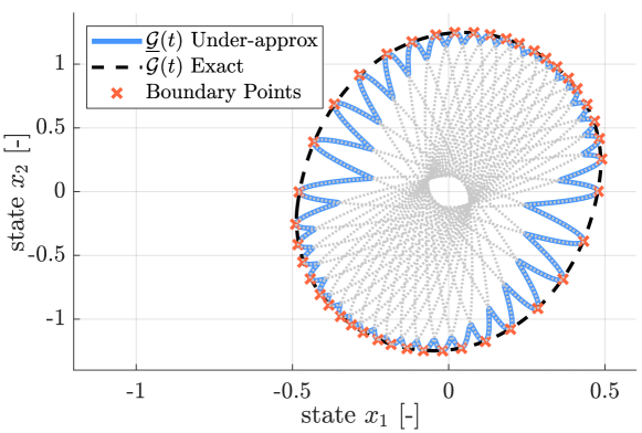
Figure 2: Comparison of the union of ellipsoids $\underline{\mathcal{G}}(t)$ and the backwards reachable set $\mathcal{G}(t)$ for (88) at time $t=0$. Grey dotted lines give the outline of each individual ellipsoid in $\underline{\mathcal{G}}(t)$. Animation: https://youtu.be/XNGjqlYKxnU.

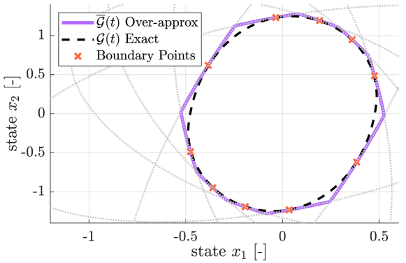
Figure 3: Comparison of the intersection of ellipsoids $\overline{\mathcal{G}}(t)$ and the backwards reachable set $\mathcal{G}(t)$ for (88) at time $t=0$. Grey dotted lines give the outline of each individual ellipsoid in $\overline{\mathcal{G}}(t)$. Animation: https://youtu.be/-0sMzyfY2GY.

A union of $n_{q}=21$ under-approximating ellipsoids $\underline{\mathcal{G}}(t)\doteq\cup^{n_{q}}_{i=1}\mathcal{E}(q_{i},Q_{i})$ for (88) was produced using Algorithm 1. A time step of $\Delta=0.01$s was selected with a minimum squared ellipsoid length of $Q_{min}=10^{-4}$. The initial set of points $\{x^{\star}_{i}\}^{n_{q}}_{i=1}$ was uniformly distributed on the boundary of $\mathcal{X}$. The boundary for $\underline{\mathcal{G}}(t)$ at time $t=0$ is presented in Fig. 2 alongside the set of points $\{x^{\star}_{i}\}^{n_{q}}_{i=1}$ which lie on the boundary of each ellipsoid $\mathcal{E}(q_{i},Q_{i})$. Due to symmetry of ellipsoids about their centre, if $x^{\star}_{i}\in\partial\mathcal{E}(q_{i},Q_{i})$ then $2q_{i}-x^{\star}_{i}\in\partial\mathcal{E}(q_{i},Q_{i})$, so these points have also been included.

Using Algorithm 2, an intersection of $n_{q}=5$ over-approximating ellipsoids $\overline{\mathcal{G}}(t)\doteq\cap^{n_{q}}_{i=1}\mathcal{E}(q_{i},Q_{i})$ for (88) was also produced with the same time step. A lower bound of $\kappa_{min}=10^{-4}$ was selected with the initial set of points $\{x^{\star}_{i}\}^{n_{q}}_{i=1}$ also uniformly distributed on $\partial\mathcal{X}$. The boundary of $\overline{\mathcal{G}}(t)$ at time $t=0$ is displayed in Fig. 3.

As guaranteed by Corollaries 3 and 4, the collection of boundary points $\{x^{\star}_{i}\}^{n_{q}}_{i=1}$ for both the under- and over-approximating collection of ellipsoids coincide with the boundary of $\mathcal{G}(t)$, yielding tight under- and over-approximations of the backwards reachable set. Note that in this example and in other tests, we have found that the condition $\underline{\Lambda}(Q_{i})<Q_{min}$ in step 14 of Algorithm 1 is never met and the condition ${\mathcal{Q}}^{\frac{1}{2}}_{i,\star}\hat{w}_{i}=0$ in step 13 of Algorithm 2 is not met so long as $x^{\star}_{i}$ is initialised with ${\mathcal{Q}}^{\frac{1}{2}}_{i,\star}\hat{w}_{i}\neq 0$. Further analysis is required to state conditions for which we can expect such a scenario to occur.

Using a fourteen-core Intel® Core^™ i7-13700H CPU, computation times in MATLAB for generating the sets $\mathcal{G}(t)$, $\underline{\mathcal{G}}(t)$, and $\overline{\mathcal{G}}(t)$ are displayed in Table 1. Their absolute and relative internal areas are also displayed. We observe that Algorithms 1 and 2 offer substantial computational savings over grid-based approaches for approximating reachable sets for LTV systems whilst capturing a comparable area. One would expect further savings in higher dimensional systems as the integration of the ellipsoids at each time step requires only a set of matrix operations, which can be performed in $\mathcal{O}(n^{3})$ time. However, more ellipsoids are likely required to obtain the same degree of conservatism in the approximating sets.

Table 1: Comparison of computation times and internal areas (at $t=0$) for $\mathcal{G}(t)$, $\underline{\mathcal{G}}(t)$, and $\overline{\mathcal{G}}(t)$.

Numerical method	Computation time [s]	Area (rel. to $\mathcal{G}(t)$)
Grid-based [8] $\mathcal{G}(t)$	19.17	1.880 (100.0%)
Algorithm 1 $\underline{\mathcal{G}}(t)$	$0.1875$	1.694 (90.09%)
Algorithm 2 $\overline{\mathcal{G}}(t)$	$0.09375$	1.974 (105.0%)

The flexibility in deciding how many ellipsoids are used in generating the under- and over-approximating sets $\underline{\mathcal{G}}(t)$ and $\overline{\mathcal{G}}(t)$ enables a trade-off to be made between the computational expense and the conservatism of the sets. In any case, states in $\underline{\mathcal{G}}(t)$ at any time $t\in[0,T]$ retain the guarantee that a constraint admissible control leading to the terminal set $\mathcal{X}$ exists. Analogously, states outside of $\overline{\mathcal{G}}(t)$ will always possess a certificate of safety, guaranteeing that the system will avoid the potentially dangerous terminal set. Approximation schemes, such as those offered here, enable reachability-based control strategies to be employed in applications where such strategies would traditionally be deemed intractable.

6 Conclusion

In this paper, we have demonstrated that viscosity supersolutions and subsolutions of a Hamilton-Jacobi-Bellman equation defined over a local domain can be used to generate under- and over-approximating reachable sets for time-varying nonlinear systems. This observation was then used to develop numerical schemes for approximating either the backwards or forwards reachable set of linear time-varying (LTV) systems.

A union and intersection of ellipsoids, which can be characterised by the minimum and maximum over a collection of quadratic functions, was proposed to under- and over-approximate the reachable set, respectively. The under-approximating ellipsoids admit a generalisation that allows for any solution of the LTV system to be contained within it. This in turn implies that it is possible to have the boundaries of the under-approximating ellipsoids and the exact reachable set coincide along a solution of the system. The over-approximating ellipsoids also admit an analogous generalisation, allowing for a tight over-approximation of the reachable set. The numerical example presented in this paper highlights a marked computational advantage afforded to LTV systems compared to grid-based approaches. Moreover, by utilising a set of conditions that are applicable to nonlinear systems and a general class of sets, the work presented here acts as a demonstration for how approximation schemes may be developed for other system classes and set representations.

Appendix

Proof of Lemma 3: First consider the statement in (13). Let $\mathscr{F}^{z}_{0}\doteq z^{-1}(\{0\})$, $\mathscr{F}^{z}_{<0}\doteq z^{-1}((-\infty,0))$, and $\mathscr{F}^{z}_{\leq 0}\doteq z^{-1}((-\infty,0])$. Fix any $\bar{x}\in\mathscr{F}^{z}_{0}$. As $z\in{\mathscr{Z}}$, there exists a sequence of points $\{x_{k}\}^{\infty}_{k=1}$ such that for each $k\in{\mathbb{N}}$, $x_{k}\in{\mathbb{B}}_{r_{k}}(\bar{x})$ with $r_{k}\doteq\textstyle{\frac{1}{k}}$ and $z(x_{k})<0$. Since $\lim_{k\rightarrow\infty}\left\lVert x_{k}-\bar{x}\right\rVert=0$ and $x_{k}\in\mathscr{F}^{z}_{<0}$ for all $k\in{\mathbb{N}}$, $\bar{x}$ is a limit point of $\mathscr{F}^{z}_{<0}$ so $\bar{x}\in\text{cl}\left(\mathscr{F}^{z}_{<0}\right)$. As $\bar{x}$ was arbitrarily selected in $\mathscr{F}^{z}_{0}$, $\mathscr{F}^{z}_{0}\subseteq\text{cl}\left(\mathscr{F}^{z}_{<0}\right)$, which implies

$$\mathscr{F}^{z}_{\leq 0}\subseteq\text{cl}\left(\mathscr{F}^{z}_{<0}\right).$$ (90)

Noting that the closure of sets preserves subset relationships and $\mathscr{F}^{z}_{\leq 0}$ is closed as it is the pre-image of a closed set under a continuous function, $\text{cl}\left(\mathscr{F}^{z}_{<0}\right)\subseteq\text{cl}(\mathscr{F}^{z}_{\leq 0})=\mathscr{F}^{z}_{\leq 0}$. Together with (90), it follows that $\text{cl}\left(\mathscr{F}^{z}_{<0}\right)=\mathscr{F}^{z}_{\leq 0}$.

Now, consider the statement in (14). Since $z$ is of class ${\mathscr{Z}}$,

$$\mathscr{F}^{z}_{0}\cap\text{int}\left(\mathscr{F}^{z}_{\leq 0}\right)=\emptyset.$$ (91)

This follows because for any $\bar{x}\in\mathscr{F}^{z}_{0}$ there can not exist an $\bar{r}>0$ such that ${\mathbb{B}}_{\bar{r}}(\bar{x})\subseteq\mathscr{F}^{z}_{0}$. Using the fact that the interior of sets preserves subset relationships, $\text{int}\left(\mathscr{F}^{z}_{<0}\right)\subseteq\text{int}\left(\mathscr{F}^{z}_{\leq 0}\right)$. Since the interior of a set is the largest open subset and $\mathscr{F}^{z}_{<0}$ is an open set, it follows that $\mathscr{F}^{z}_{<0}\subseteq\text{int}\left(\mathscr{F}^{z}_{\leq 0}\right)$. Moreover, for any $\bar{x}\in\text{int}\left(\mathscr{F}^{z}_{\leq 0}\right)$ either $\bar{x}\in\mathscr{F}^{z}_{0}$ or $\mathscr{F}^{z}_{<0}$, which means (91) implies $\text{int}\left(\mathscr{F}^{z}_{\leq 0}\right)\subseteq\mathscr{F}^{z}_{<0}$. Thus, $\mathscr{F}^{z}_{<0}=\text{int}\left(\mathscr{F}^{z}_{\leq 0}\right)$. ∎

Proof of Lemma 4: Fix any $t\in[0,T]$ and any point $x_{0}\in\{x\in{\mathbb{R}}^{n}\,|\,v(t,x)=0\}$. Since $f$ satisfies Assumption 2, the infimum in (4) is attained (use Theorem 7.1.4 of [28]). In particular, there exists a $u^{\star}\in{\mathscr{U}}[t,T]$ such that $g(\varphi(T;t,x_{0},u^{\star}))=v(t,x_{0})=0$. Let $x^{\star}(\cdot)\doteq\varphi(\cdot;t,x_{0},u^{\star})$ be the solution of (1) corresponding to $u^{\star}$. The proof proceeds by demonstrating that $x_{0}$ must be arbitrarily close to a point in $\{x\in{\mathbb{R}}^{n}\,|\,v(t,x)<0\}$ since $x^{\star}(T)=\varphi(T;t,x_{0},u^{\star})$ is arbitrarily close to a point in $g^{-1}((-\infty,0))$. To see this, first note that from uniqueness of solutions of (1),

$$x^{\star}(s)\doteq\varphi(s;t,x_{0},u^{\star})=\varphi(s;T,x^{\star}(T),u^{\star}),\quad\forall s\in[t,T],$$

since $x^{\star}(\cdot)$ and $\varphi(\cdot;T,x^{\star}(T),u^{\star})$ share the same control and terminal condition $x^{\star}(T)$. Then, by continuity of solutions of (1), for any $r>0$ there exists a $\bar{r}>0$ such that

$$\left\lVert\varphi(t;T,\bar{x},u^{\star})-x^{\star}(t)\right\rVert=\left\lVert\varphi(t;T,\bar{x},u^{\star})-x_{0}\right\rVert<r,$$ (92)

whenever $\left\lVert\bar{x}-x^{\star}(T)\right\rVert<\bar{r}$. Moreover, since $x^{\star}(T)\in g^{-1}(\{0\})$ and $g$ is of class ${\mathscr{Z}}$, given any $\bar{r}>0$, the set ${\mathbb{B}}_{\bar{r}}(x^{\star}(T))\cap g^{-1}((-\infty,0))$ is non-empty. Then, take any $\bar{x}\in{\mathbb{B}}_{\bar{r}}(x^{\star}(T))\cap g^{-1}((-\infty,0))$ to obtain

$$v(t,\varphi(t;T,\bar{x},u^{\star}))=\inf_{u\in{\mathscr{U}}[t,T]}g\left(\varphi(T;t,\varphi(t,T,\bar{x},u^{\star}),u)\right){}$$

$$\qquad\leq g\left(\varphi(T;t,\varphi(t;T,\bar{x},u^{\star}),u^{\star})\right)=g(\bar{x})<0.$$ (93)

From (92) and (93), it follows that for any $r>0$ there exists a point in ${\mathbb{B}}_{r}(x_{0})$ that also lies in $\{x\in{\mathbb{R}}^{n}\,|\,v(t,x)<0\}$. As $x_{0}\in\{x\in{\mathbb{R}}^{n}\,|\,v(t,x)=0\}$ is arbitrary, the map $x\mapsto v(t,x)$ is of class ${\mathscr{Z}}$ for all $t\in[0,T]$. ∎

Proof of Lemma 8: Fix any $t\in[0,T]$ and $\bar{x}\in\{x\in{\mathbb{R}}^{n}\,|\,\overline{e}(t,x)=0\}$. As $Q_{i}(t)\in\mathbb{S}^{n}_{>0}$ implies $Q_{i}(t)$ is invertible, $\overline{e}$ in (39) is well-defined. Omitting time-dependence for brevity, there exists an $\bar{n}\doteq\bar{n}(t,\bar{x})\in\{1,\ldots,n_{q}\}$ such that

$$\left\langle\bar{x}-q_{\bar{n}},Q^{-1}_{\bar{n}}(\bar{x}-q_{\bar{n}})\right\rangle-1=0\iff\big{\lVert}Q^{-\frac{1}{2}}_{\bar{n}}(\bar{x}-q_{\bar{n}})\big{\rVert}_{2}=1.$$ (94)

Fix any $r>0$ and let $\tilde{x}\doteq\bar{x}-\frac{a}{2}\cdot\frac{\bar{x}-q_{\bar{n}}}{\lVert\bar{x}-q_{\bar{n}}\rVert_{2}}$ with $a\doteq\min\{r,\lVert\bar{x}-q_{\bar{n}}\rVert_{2}\}>0$. Note that $\tilde{x}$ is well defined as $\bar{x}\neq q_{\bar{n}}$. Since $0<a<\big{\lVert}\bar{x}-q_{\bar{n}}\big{\rVert}_{2}$,

$$\tfrac{1}{2}<1-\frac{a}{2\lVert\bar{x}-q_{\bar{n}}\rVert_{2}}<1.$$ (95)

From (94), (95), and the definition of $\tilde{x}$,

$$\big{\lVert}Q^{-\frac{1}{2}}_{\bar{n}}(\tilde{x}-q_{\bar{n}})\big{\rVert}_{2} =\Big{(}1-\tfrac{a}{2\lVert\bar{x}-q_{\bar{n}}\rVert_{2}}\Big{)}\big{\lVert}Q^{-\frac{1}{2}}_{\bar{n}}(\bar{x}-q_{\bar{n}})\big{\rVert}_{2}<1$$

$$\implies \left\langle\tilde{x}-q_{\bar{n}},Q^{-1}_{\bar{n}}(\tilde{x}-q_{\bar{n}})\right\rangle<1.$$

By definition (39), $\overline{e}(t,\tilde{x})\leq\left\langle\tilde{x}-q_{\bar{n}},Q^{-1}_{\bar{n}}(\tilde{x}-q_{\bar{n}})\right\rangle-1<0$. Since $\lVert\tilde{x}-\bar{x}\rVert_{2}=\frac{a}{2}<r$, which means $\tilde{x}\in{\mathbb{B}}_{r}(\bar{x})$, it follows that for any $\bar{x}\in\{x\in{\mathbb{R}}^{n}\,|\,\overline{e}(t,x)=0\}$ and any $r>0$, there exists a point $\tilde{x}\in{\mathbb{B}}_{r}(\bar{x})$ with $\overline{e}(t,\tilde{x})<0$. Hence, as $t$ is arbitrary, $x\mapsto\overline{e}(t,x)$ is of class ${\mathscr{Z}}$ for all $t\in[0,T]$. ∎

References

• [1] B. Schurmann, M. Klischat, N. Kochdumper, and M. Althoff, “Formal safety net control using backward reachability analysis,” IEEE Trans. on Automatic Control, 2021.
• [2] M. Chen, Q. Hu, J. F. Fisac, K. Akametalu, C. Mackin, and C. J. Tomlin, “Reachability-based safety and goal satisfaction of unmanned aerial platoons on air highways,” Journal of Guidance, Control, and Dynamics, vol. 40, no. 6, pp. 1360–1373, 2017.
• [3] C. Llanes, M. Abate, and S. Coogan, “Safety from fast, in-the-loop reachability with application to UAVs,” in 2022 ACM/IEEE 13th International Conference on Cyber-Physical Systems (ICCPS).   IEEE, 2022, pp. 127–136.
• [4] Y. Zhou and J. S. Baras, “Reachable set approach to collision avoidance for uavs,” in 2015 54th IEEE Conference on Decision and Control (CDC).   IEEE, 2015, pp. 5947–5952.
• [5] M. Chen and C. J. Tomlin, “Hamilton-Jacobi reachability: Some recent theoretical advances and applications in unmanned airspace management,” Annual Review of Control, Robotics, and Autonomous Systems, vol. 1, pp. 333–358, 2018.
• [6] I. M. Mitchell, A. M. Bayen, and C. J. Tomlin, “A time-dependent Hamilton-Jacobi formulation of reachable sets for continuous dynamic games,” IEEE Trans. on Automatic Control, vol. 50, no. 7, pp. 947–957, 2005.
• [7] A. Altarovici, O. Bokanowski, and H. Zidani, “A general Hamilton-Jacobi framework for non-linear state-constrained control problems,” ESAIM: Control, Optimisation and Calculus of Variations, vol. 19, no. 2, pp. 337–357, 2013.
• [8] I. M. Mitchell. A toolbox of level set methods. [Online]. Available: https://www.cs.ubc.ca/ mitchell/ToolboxLS/
• [9] F. Borrelli, A. Bemporad, and M. Morari, Predictive control for linear and hybrid systems.   Cambridge University Press, 2017.
• [10] L. Yang and N. Ozay, “Scalable zonotopic under-approximation of backward reachable sets for uncertain linear systems,” IEEE Control Systems Letters, vol. 6, pp. 1555–1560, 2021.
• [11] A. Girard, “Reachability of uncertain linear systems using zonotopes,” in HSCC, vol. 3414.   Springer, 2005, pp. 291–305.
• [12] A. Halder, “Smallest ellipsoid containing $p$-sum of ellipsoids with application to reachability analysis,” IEEE Trans. on Automatic Control, vol. 66, no. 6, pp. 2512–2525, 2020.
• [13] N. Shishido and C. J. Tomlin, “Ellipsoidal approximations of reachable sets for linear games,” in Proceedings of the 39th IEEE Conference on Decision and Control, vol. 1.   IEEE, 2000, pp. 999–1004.
• [14] S. Kousik, A. Dai, and G. X. Gao, “Ellipsotopes: Uniting ellipsoids and zonotopes for reachability analysis and fault detection,” IEEE Trans. on Automatic Control, 2022.
• [15] C. Le Guernic and A. Girard, “Reachability analysis of linear systems using support functions,” Nonlinear Analysis: Hybrid Systems, vol. 4, no. 2, pp. 250–262, 2010.
• [16] M. Althoff and B. H. Krogh, “Reachability analysis of nonlinear differential-algebraic systems,” IEEE Trans. on Automatic Control, vol. 59, no. 2, pp. 371–383, 2013.
• [17] D. Goswami and D. A. Paley, “Bilinearization, reachability, and optimal control of control-affine nonlinear systems: A koopman spectral approach,” IEEE Trans. on Automatic Control, vol. 67, no. 6, pp. 2715–2728, 2021.
• [18] M. Chen, S. L. Herbert, M. S. Vashishtha, S. Bansal, and C. J. Tomlin, “Decomposition of reachable sets and tubes for a class of nonlinear systems,” IEEE Trans. on Automatic Control, vol. 63, no. 11, pp. 3675–3688, 2018.
• [19] S. Coogan, “Mixed monotonicity for reachability and safety in dynamical systems,” in 2020 59th IEEE Conference on Decision and Control (CDC).   IEEE, 2020, pp. 5074–5085.
• [20] V. Rubies-Royo, D. Fridovich-Keil, S. Herbert, and C. J. Tomlin, “A classification-based approach for approximate reachability,” in 2019 International Conference on Robotics and Automation (ICRA).   IEEE, 2019, pp. 7697–7704.
• [21] K. D. Julian and M. J. Kochenderfer, “Reachability analysis for neural network aircraft collision avoidance systems,” Journal of Guidance, Control, and Dynamics, vol. 44, no. 6, pp. 1132–1142, 2021.
• [22] A. Alla, P. M. Dower, and V. Liu, “A tree structure approach to reachability analysis,” in Advances in Numerical Methods for Hyperbolic Balance Laws and Related Problems.   Springer, 2023, pp. 1–21.
• [23] V. Liu, C. Manzie, and P. M. Dower, “Reachability of linear time-invariant systems via ellipsoidal approximations,” IFAC-PapersOnLine, vol. 56, no. 1, pp. 126–131, 2023.
• [24] V. Sinyakov, “Method for computing exterior and interior approximations to the reachability sets of bilinear differential systems,” Differential Equations, vol. 51, pp. 1097–1111, 2015.
• [25] A. B. Kurzhanski and P. Varaiya, “Ellipsoidal techniques for reachability analysis: internal approximation,” Systems & Control Letters, vol. 41, no. 3, pp. 201–211, 2000.
• [26] A. Kurzhanski and P. Varaiya, “Reachability analysis for uncertain systems-the ellipsoidal technique,” Dynamics of Continuous Discrete and Impulsive Systems Series B, vol. 9, pp. 347–368, 2002.
• [27] H. K. Khalil, Nonlinear systems third edition.   Prentice Hall, 2002, vol. 115.
• [28] P. Cannarsa and C. Sinestrari, Semiconcave functions, Hamilton-Jacobi equations, and optimal control.   Springer Science & Business Media, 2004, vol. 58.
• [29] M. Bardi, I. C. Dolcetta et al., Optimal control and viscosity solutions of Hamilton-Jacobi-Bellman equations.   Springer, 1997, vol. 12.
• [30] I. M. Mitchell, “Comparing forward and backward reachability as tools for safety analysis,” in International Workshop on Hybrid Systems: Computation and Control.   Springer, 2007, pp. 428–443.
• [31] M. G. Crandall and P.-L. Lions, “Viscosity solutions of Hamilton-Jacobi equations,” Transactions of the American mathematical society, vol. 277, no. 1, pp. 1–42, 1983.
• [32] A. Y. Kruger, “On Fréchet subdifferentials,” Journal of Mathematical Sciences, vol. 116, no. 3, pp. 3325–3358, 2003.
• [33] R. T. Rockafellar and R. J. B. Wets, Variational analysis.   Springer Science & Business Media, 2009, vol. 317.
• [34] W. H. Fleming and H. M. Soner, Controlled Markov processes and viscosity solutions.   Springer Science & Business Media, 2006, vol. 25.
• [35] A. G. Constantine and J. C. Grower, “Some properties and applications of simple orthogonal matrices,” IMA Journal of Applied Mathematics, vol. 21, no. 4, pp. 445–454, 1978.
• [36] M. Behr, P. Benner, and J. Heiland, “Solution formulas for differential Sylvester and Lyapunov equations,” Calcolo, vol. 56, no. 4, p. 51, 2019.