Extreme Compression of Large Language Models via Additive Quantization

Abstract

The emergence of accurate open large language models (LLMs) has led to a race towards performant quantization techniques which can enable their execution on end-user devices. In this paper, we revisit the problem of “extreme” LLM compression—defined as targeting extremely low bit counts, such as 2 to 3 bits per parameter—from the point of view of classic methods in Multi-Codebook Quantization (MCQ). Our algorithm, called AQLM, generalizes the classic Additive Quantization (AQ) approach for information retrieval to advance the state-of-the-art in LLM compression, via two innovations: 1) learned additive quantization of weight matrices in input-adaptive fashion, and 2) joint optimization of codebook parameters across entire layer blocks. Broadly, AQLM is the first scheme that is Pareto optimal in terms of accuracy-vs-model-size when compressing to less than 3 bits per parameter, and significantly improves upon all known schemes in the extreme compression (2bit) regime. In addition, AQLM is practical: we provide fast GPU and CPU implementations of AQLM for token generation, which enable us to match or outperform optimized FP16 implementations for speed, while executing in a much smaller memory footprint.

1 Introduction

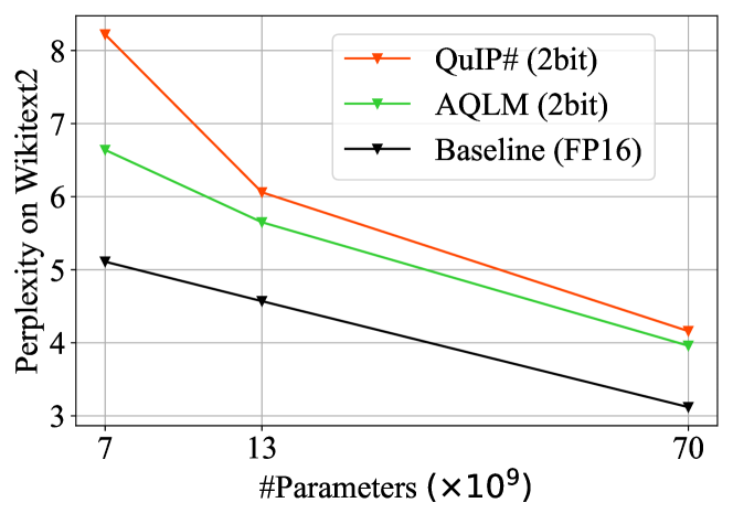
Figure 1: Comparison of AQLM (2-bit) relative to the state-of-the-art QuIP# (2-bit) and the original 16-bit weights on Llama 2 7, 13, and 70B models.

The rapid advancement of generative large language models (LLMs) has led to massive industrial and popular interest, driven in part by the availability of accurate open LLMs, such as Llama 1 and 2 (Touvron et al., 2023), Falcon (TII UAE, 2023), BLOOM (Scao et al., 2022), OPT (Zhang et al., 2022), or NeoX/Pythia (Biderman et al., 2023). A key advantage of open models is that they can be inferenced or fine-tuned locally by end-users, assuming that their computational and memory costs can be reduced to be manageable on commodity hardware. This has led to several methods for inference and fine-tuning on compressed LLMs (Dettmers et al., 2022; Frantar et al., 2022a; Dettmers & Zettlemoyer, 2022; Lin et al., 2023; Dettmers et al., 2023a). Currently, the primary approach for accurate post-training compression of LLMs is quantization, which reduces the bit-width at which model weights (and possibly activations) are stored, leading to improvements in model footprint and memory transfer.

By and large, LLM weights are compressed via “direct” quantization, in the sense that a suitable quantization grid and normalization are first chosen for each matrix sub-component, and then weights are each mapped onto the grid either by direct rounding, e.g. (Dettmers & Zettlemoyer, 2022), or via more complex allocations, e.g. (Frantar et al., 2022a). Quantization induces a natural compression-vs-accuracy trade-off, usually measured in terms of model size vs model perplexity (PPL). Existing approaches can achieve arguably low accuracy loss at 3-4 bits per element (Dettmers et al., 2023b; Chee et al., 2023; Kim et al., 2023), and can even stably compress models to 2 or even less bits per element, in particular, for extremely large models (Frantar & Alistarh, 2023). Yet, in most cases, low bit counts come at the cost of significant drops in accuracy, higher implementation complexity and runtime overheads. Specifically, from the practical perspective, “extreme” quantization in the 2-bit range using current techniques is inferior to simply using a smaller base model and quantizing it to higher bitwidths, such as 3-4 bits per parameter, as the latter yields higher accuracy given the same model size in bytes (Dettmers & Zettlemoyer, 2022; Chee et al., 2023).

Contribution. In this work, we improve the state-of-the-art in LLM compression by showing for the first time that Multi-Codebook Quantization (MCQ) techniques can be extended to LLM weight compression. Broadly, MCQ is a family of information retrieval methods (Chen et al., 2010; Jegou et al., 2010; Ge et al., 2013; Zhang et al., 2014; Babenko & Lempitsky, 2014; Martinez et al., 2016, 2018), consisting of specialized quantization algorithms to compress databases of vectors, allowing for efficient search. Unlike direct quantization, MCQ compresses multiple values jointly, by leveraging the mutual information of quantized values.

More precisely, we extend Additive Quantization (AQ) (Babenko & Lempitsky, 2014; Martinez et al., 2016), a popular MCQ algorithm, to the task of compressing LLM weights such that the output of each layer and Transformer block are approximately preserved. Our extension reformulates the classic AQ optimization problem to reduce the error in LLM layer outputs under the input token distribution and as well as to jointly optimize codes over layer blocks, rather than only preserving the weights themselves as in standard AQ. We refer to the resulting procedure as Additive Quantization of Language Models (AQLM). Unlike some extreme LLM quantization approaches that require hybrid sparse-quantized formats which separate outlier quantization (Kim et al., 2023; Dettmers et al., 2023b), AQLM quantizes models in a simple homogeneous format, which is easy to support in practice. Our main contributions are as follows:

1. We propose the AQLM algorithm, which extends AQ to post-training compression of LLM weights, via two innovations: (1) adapting the MAP-MRF optimization problem behind AQ to be instance-aware, taking layer calibration input & output activations into account; (2) complementing the layer-wise optimization with an efficient intra-layer tuning technique, which optimizes quantization parameters jointly over several layers, using only the calibration data.

2. We evaluate the effectiveness of this algorithm on the task of compressing accurate open LLMs from the Llama 2 (Touvron et al., 2023) family with compression rates of 2-4 bits per parameter. We find that AQLM outperforms the previous state-of-the-art across the standard 2-4 bit compression range, with the most significant improvements for extreme 2-bit quantization (see Figure 1). We provide detailed ablations for the impact of various algorithm parameters, such as code width and number of codebooks, and extend our analysis to the recent Mixtral model (Jiang et al., 2024).

3. We show that AQLM is practical, by providing efficient GPU and CPU kernels implementations for specific encodings, as well as end-to-end generation. Results show show that our approach can match or even outperform the floating point baseline in terms of speed, while reducing the memory footprint by up to 8x. Specifically, AQLM can be executed with layer-wise speedups of $\sim 30\%$ for GPUs, and of up to 4x for CPU inference.

2 Background & Related Work

2.1 LLM Quantization

Early efforts towards post-training quantization (PTQ) methods (Nagel et al., 2020; Gholami et al., 2021) that scale to LLMs such as ZeroQuant (Yao et al., 2022), LLM.int8() (Dettmers et al., 2022), and nuQmm (Park et al., 2022) employed direct round-to-nearest (RTN) projections, and adjusted quantization granularity to balance memory efficiency and accuracy. GPTQ (Frantar et al., 2022a) proposed a more accurate data-aware approach via an approximate large-scale solver for minimizing layer-wise $\ell_{2}$ errors.

Dettmers & Zettlemoyer (2022) examined the accuracy-compression trade-offs of these early methods, suggesting that 4-bit quantization may be optimal for RTN quantization, and observing that data-aware methods like GPTQ allow for higher compression, i.e. strictly below 4 bits/weight, maintaining Pareto optimality. Our work brings this Pareto frontier below 3 bits/weight, for the first time. Parallel work quantizing both weights and activations to 8-bits, by Dettmers et al. (2022), Xiao et al. (2022), and Yao et al. (2022) noted that the “outlier features” in large LLMs cause substantial errors, prompting various mitigation strategies.

Recently, several improved techniques have focused on the difficulty of quantizing weight outliers, which have high impact on the output error. SpQR (Dettmers et al., 2023b) addresses this by saving outliers as a highly-sparse higher-precision matrix. AWQ (Lin et al., 2023) reduces the error of quantizing channels with the highest activation magnitudes by employing per-channel scaling to reduce the error on important weights. SqueezeLLM (Kim et al., 2023) uses the diagonal Fisher as a proxy for the Hessian and implements non-uniform quantization through K-means clustering.

The state-of-the-art method in terms of accuracy-to-size trade-off is QuIP (Chee et al., 2023). Concurrent to our work, an improved variant called QuIP# (Tseng et al., 2023) was introduced. Roughly, these methods work by first “smoothening” weights by multiplying with a rotation matrix, and then mapping them onto a lattice. QuIP was the first method to obtain stable results (i.e., single-digit PPL increases) in the 2-bit per parameter compression range. At a high level, QuIP and QuIP# aim to minimize the “worst-case” error for each layer, given initial weights and calibration data. For instance, in QuIP#, the distribution of the rotated weights approximates a Gaussian, while the encoding lattice (E8P) is chosen to minimize “rounding” error. By contrast, our approach uses a different weight encoding (codebooks are additive), and learned codebooks instead of a fixed codebook. Thus, our insight is that we should be able to obtain higher accuracy by direct optimization of the codebooks over the calibration set, removing the rotation. Further, we show that codebooks for different layers can co-train via joint fine-tuning over the calibration data.

2.2 Quantization for Nearest Neighbor Search

Our work builds on approximate nearest neighbor search (ANN) algorithms. Unlike PTQ, ANN quantization aims to compress a database of vectors to allow a user to efficiently compute similarities and find nearest neighbors relative to a set of query points. For high compression, modern ANN search algorithms employ vector quantization (VQ)—which quantizes multiple vector dimensions jointly (Burton et al., 1983; Gray, 1984). It achieves this by learning “codebooks”: i.e. a set of learnable candidate vectors that can be used to encode the data. To encode a given database vector, VQ splits it into sub-groups of entries, then encodes every group by choosing a vector from the learned codebook. The algorithm efficiently computes distances or dot-products for similarity search by leveraging the linearity of dot products.

Quantization methods for ANN search generalize vector quantization and are referred to as multi-codebook quantization (MCQ). MCQ methods typically do not involve information loss on the query side, which makes them the leading approach for memory-efficient ANN (Ozan et al., 2016; Martinez et al., 2018). We briefly review MCQ below.

Product quantization (PQ) (Jegou et al., 2010) is an early version of MCQ, which encodes each vector $x\in\mathbf{R}^{D}$ as a concatenation of $M$ codewords from $M$ $\frac{D}{M}$-dimensional codebooks $C_{1},\ldots,C_{M}$, each containing $K$ codewords. PQ decomposes a vector into $M$ separate subvectors and applies vector quantization (VQ) to each subvector, while using a separate codebook. Thus, each vector $x$ is encoded by a tuple of codeword indices $[i_{1},\ldots,i_{M}]$ and approximated by $x\approx[c_{1i_{1}},\ldots,c_{Mi_{M}}]$. Fast Euclidean distance computation becomes possible using lookup tables:

$$\|q-x\|^{2}\approx\|q-[c_{1i_{1}},\ldots,c_{Mi_{M}}]\|^{2}=\sum\limits_{m=1}^{M}{\|q_{m}-c_{mi_{m}}\|}^{2},$$

where $q_{m}$ is the $m$th subvector of a query $q$. This sum can be calculated using $M$ additions and lookups if the distances from query subvectors to codewords are precomputed. Since product-based approximations work better if the $\frac{D}{M}$-dimensional components independent distributions, subsequent work has looked into finding better transformations (Ge et al., 2013; Norouzi & Fleet, 2013). As for the other similarity functions, (Guo et al., 2016) proposes a quantization procedure for maximum inner product search (MIPS). They minimize quantization error in the inner products between database and query vectors by solving a constrained optimization problem. Similarly to the formula above, this procedure allows for efficient inner product search by precomputing dot products between the query $q$ an all codes in the learned codebooks, then adding these partial dot products to recover the full similarity score.

Non-orthogonal quantizations. Follow-up work (Chen et al., 2010; Babenko & Lempitsky, 2014; Martinez et al., 2016; Zhang et al., 2014; Ozan et al., 2016; Martinez et al., 2018) generalized the idea of Product Quantization by approximating each vector by a sum of $M$ codewords instead of concatenation. The resulting procedure is still efficient while the approximation accuracy is increased.

For this, Residual Vector Quantization (Chen et al., 2010), quantizes original vectors, and then iteratively quantizes the approximation residuals from the previous iteration. Additive Quantization (AQ) (Babenko & Lempitsky, 2014) is more general, as it does not impose constraints on the codewords from the different codebooks. Usually, AQ provides the smallest compression errors, but is more complex to train for large $M$. We discuss this in detail in Section 3.

Finally, several recent works (Martinez et al., 2016, 2018; Zhang et al., 2014) elaborate the idea of Additive Quantization, proposing the more effective procedure for codebooks learning. Composite Quantization (CQ) (Zhang et al., 2014) learns codebooks with a fixed value of scalar product between the codewords from different codebooks. Currently, the state-of-the-art compression accuracy is achieved by the LSQ method (Martinez et al., 2018).

Vector quantization for model compression.

There has been significant work on exploiting vector quantization in the context of machine learning. For instance, Zhou et al. (2017); Li et al. (2017); Chen et al. (2019) use multi-codebook quantization to compress word embeddings within deep learning models. Another line of work (Blalock & Guttag, 2021; McCarter & Dronen, 2022; Fernández-Marqués et al., 2023) explores vector quantization for linear models, or linear layers within deep models. Similarly to PQ above, these techniques pre-compute inner products between inputs and all codes, then compute linear layer via look-up, which speeds up inference. However, these algorithms introduce significant prediction error that does not allow them to compress deep models. Thus, we believe we are the first to successfully adapt and scale MCQ to LLMs.

3 AQLM: Additive Quantization for LLMs

3.1 Overview

We start from the observation that additive quantization (AQ) solves a related problem to post-training quantization (PTQ) (Nagel et al., 2020; Frantar et al., 2022b): both settings assume the existence of a set of “input” vectors, i.e. input data for AQ, and the weight matrix rows for PTQ. The goal is to compress these inputs while preserving dot product similarity, against query vectors (for AQ), and against layer input embeddings (for PTQ). The difference between the two is that AQ assumes that the distribution of queries is unknown, whereas PTQ methods, e.g. (Frantar et al., 2022b), show that it is sufficient to optimize for sample input embeddings from a set of calibration data.

At a high level, we start by solving the following problem: for a linear layer with $d_{in}$ input and $d_{out}$ output features given its weights $\mathbf{W}\in\mathbb{R}^{d_{out}\times d_{in}}$ and a set of calibration inputs $\mathbf{X}\in\mathbb{R}^{d_{in}\times n}$, one seeks for a configuration of quantized weights $\hat{W}$ that optimizes squared error between the output of the original and compressed layer:

$$\underset{\widehat{\mathbf{W}}}{\arg\min}||\mathbf{W}\mathbf{X}-\widehat{\mathbf{W}}\mathbf{X}||_{2}^{2}.$$ (1)

In the following, we will assume that $\widehat{\mathbf{W}}$ is quantized using AQ, and adopt standard notation (Martinez et al., 2016). AQ splits weight rows into groups of $g$ consecutive elements, and represents each group of weights as a sum of $M$ vectors chosen from multiple learned codebooks $C_{1},...C_{M}$, each containing $2^{B}$ vectors (for B-bit codes). A weight is encoded by choosing a single code from each codebook and summing them up. We denote this choice as a one-hot vector $b_{m}$, which results in the following representation for a group: $\sum_{m=1}^{M}C_{m}b_{ijm}$. This is similar to PTQ algorithms (Frantar et al., 2022a), except for using much more complex coding per group. To represent the full weights, we simply concatenate:

$$\widehat{\mathbf{W}}_{i}{=}\sum_{m=1}^{M}C_{m}b_{i,1,m}\oplus...\oplus\sum_{m=1}^{M}C_{m}b_{i,d_{in}/g,m},$$ (2)

where $\oplus$ denotes concatenation and $b_{ijm}\in\mathbb{R}^{2^{B}}$ represents a one-hot code for the $i$-th output unit, $j$-th group of input dimensions and $m$-th codebook.

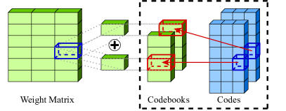
Figure 2: Groups of weights are represented by a sum of codes selected from codebooks by corresponding indices.

Our algorithm will learn codebooks $C_{m}\in\mathbb{R}^{g\times 2^{B}}$ and the discrete codes represented by one-hot $b\in\mathbb{R}^{d_{out}\times d_{in}/g\times M\times 2^{B}}$. The resulting scheme encodes each group of $g$ weights using $M\cdot B$ bits and further requires $g\cdot 2^{B}\cdot 16$ bits for FP16 codebooks. The error becomes:

$$\underset{C,b}{\arg\min}||\mathbf{W}\mathbf{X}-\left(\text{Concat}_{i,j}\sum^{M}_{m=1}C_{m}b_{i,j,m}\right)\mathbf{X}||_{2}^{2}.$$ (3)

To learn this weight representation, we initialize codebooks $C$ and codes $b$ by running residual K-means as in Chen et al. (2010). Then, we alternate between updating codes $b_{i,j,m}$ and codebooks $C_{m}$ until the loss function (3) stops improving up to the specified tolerance. Since codes are discrete and codebooks are continuous, and we are optimizing over multiple interacting layers, our approach has three phases, described in Algorithm 1 and detailed below.

3.2 Phase 1: Beam search for codes

First, AQLM updates the codes $b_{i,j,m}$ to minimize the MSE objective (3). Similarly to Babenko & Lempitsky (2014); Martinez et al. (2016, 2018), we reformulate the objective in terms of a fully-connected discrete Markov Random Field (MRF) to take advantage of MRF solvers.

To simplify the derivation, let us first consider a special case of a single output unit ($d_{out}{=}1)$ and a single quantization group (i.e. $g{=}d_{in}$), to get rid of the concatenation operator: $||\mathbf{W}\mathbf{X}-\sum^{M}_{m=1}C_{m}b_{m}\mathbf{X}||_{2}^{2}$. We rewrite this objective by expanding the squared difference:

$$||\mathbf{W}\mathbf{X}-\sum^{M}_{m=1}C_{m}b_{m}\mathbf{X}||_{2}^{2}=||\mathbf{W}\mathbf{X}||_{2}^{2}-\\ -2\left\langle\mathbf{W}\mathbf{X}\ \ ,\ \ \sum^{M}_{m=1}C_{m}b_{m}\mathbf{X}\right\rangle_{F}+||\sum^{M}_{m=1}C_{m}b_{m}\mathbf{X}||_{2}^{2}$$ (4)

Above, $\langle\cdot,\cdot\rangle_{F}$ denotes a Frobenius inner product of two matrices. Next, let us consider the three components of Eqn. (4) in isolation. First, note that $||\mathbf{W}\mathbf{X}||_{2}^{2}$ is constant in $b$ and can be ignored. The second component can be expanded further into pairwise dot products:

$$||\sum^{M}_{m=1}C_{m}b_{m}\mathbf{X}||_{2}^{2}=\sum^{M}_{i=1}\sum^{M}_{j=1}\left\langle C_{i}b_{i}\mathbf{X},C_{j}b_{j}\mathbf{X}\right\rangle_{F}.$$ (5)

Note that both the second and third components rely on Frobenius products of $C_{m}b_{m}\mathbf{X}$-like matrices. These matrices can be inconvenient in practice: since $\mathbf{X}\in\mathbb{R}^{d_{in}\times n}$, the size of each matrix will scale with the size of calibration dataset $n$. To circumvent this, we rewrite the products as:

$$\left\langle C_{i}b_{i}\mathbf{X},C_{j}b_{j}\mathbf{X}\right\rangle_{F}=\left\langle C_{i}b_{i}\mathbf{X}\mathbf{X}^{T},C_{j}b_{j}\right\rangle_{F}.$$ (6)

Thus one can pre-compute $\mathbf{X}\mathbf{X}^{T}\in\mathbb{R}^{d_{in}\times d_{in}}$. We will denote this type of product as $\left\langle\mathbf{A},\mathbf{B}\right\rangle_{\mathbf{X}\mathbf{X}^{T}}\stackrel{{\scriptstyle\mathsf{def}}}{{=}}\left\langle\mathbf{A}\mathbf{X}\mathbf{X}^{T},\mathbf{B}\right\rangle_{F}$ in future derivations. Then, Eqn. (4) becomes:

$$||\mathbf{W}\mathbf{X}-\sum^{M}_{m=1}C_{m}b_{m}\mathbf{X}||_{2}^{2}=||\mathbf{W}\mathbf{X}||_{2}^{2}-\\ -2\sum^{M}_{m=1}\left\langle\mathbf{W},C_{m}b_{m}\right\rangle_{\mathbf{XX}^{T}}+\sum^{M}_{i=1}\sum^{M}_{j=1}\left\langle C_{i}b_{i},C_{j}b_{j}\right\rangle_{\mathbf{XX}^{T}}.$$ (7)

Finally, we generalize this equation to multiple output units ($d_{out}>1$) and quantization groups ($g{\neq}d_{in}$). For $d_{out}>1$, note that the original objective (3) is additive with respect to output units: thus, we can apply (7) independently to each output dimension and sum up results. To support multiple input groups ($g{\neq}d_{in}$), we can treat each group as a separate codebook where only the codes for the active group are nonzero. Thus, we need to repeat each codebook $d_{in}/g$ times and pad it with zeros according to the active group.

It is now evident that minimizing (4) is equivalent to MAP inference in a Markov Random Field with $\left\langle\mathbf{W},C_{m}b_{m}\right\rangle_{\mathbf{XX}^{T}}$ as unary potentials and $\left\langle C_{i}b_{i},C_{j}b_{j}\right\rangle_{\mathbf{XX}^{T}}$ as pairwise potentials. While finding the exact optimum is infeasible, prior work has shown that this type of MRF can be solved approximately via beam search or ICM (Besag, 1986).

To solve this problem, we chose to adapt a beam search algorithm from Babenko & Lempitsky (2014). This algorithm maintains a beam of $k$ (beam size) best configurations for the codes, starting from the previous solution. On each step, the algorithm attempts to replace one code by trying all $2^{B}k$ alternatives and selecting the $k$ best based on MSE (7).

Since the loss function is additive, changing one code only affects a small subset of loss components. Thus, we can compute the loss function efficiently by starting with a previous loss function (before code replacement), then adding and subtracting the components that changed during this iteration. These few loss components can be computed efficiently by multiplying with $\mathbf{X}\mathbf{X}^{T}$ ahead of beam search. The beam search runs over all $d_{out}$ output units in parallel. This is possible because encoding one output unit does not affect the objective (7) of other units. Note that beam search is not necessarily the best solution to this problem. AQ variants for retrieval (Martinez et al., 2016, 2018) use randomized ICM to find solutions faster. In this study, we chose beam search because it was easier to implement in ML frameworks like PyTorch/JAX.

3.3 Phase 2: Codebook update

In the second phase, we find the optimal codebook vectors $C_{1},...,C_{M}$ that minimize the same squared error as the beam search. If we treat the codes $b$ as constants, minimizing (3) becomes a least squares problem for $C_{m}$. The original AQ algorithm solves this problem in closed form, relying on the fact that each vector dimension can be optimized independently. Our problem is complicated due to the presence of $\mathbf{X}\mathbf{X}^{T}$: the optimal value of one codebook coordinate depends on the values of all others. In principle, we could optimize $C_{m}$ in closed form, but it would require inverting a large matrix, or using iterative least squares solvers (e.g. conjugate gradients) specialized to this problem.

For simplicity, our current implementation defaults to using Adam (Kingma & Ba, 2015) for approximately solving this minimization problem. In practice, this codebook tuning phase takes up a small fraction of the total compute time. We compute the objective as follows:

$$||\mathbf{WX}-\widehat{\mathbf{W}}\mathbf{X}||_{2}^{2}=||(\mathbf{W}-\widehat{\mathbf{W}})\mathbf{X}||_{2}^{2}=\\ =\left\langle(\mathbf{W}-\widehat{\mathbf{W}})\mathbf{X}\mathbf{X}^{T},(\mathbf{W}-\widehat{\mathbf{W}})\right\rangle_{F},$$ (8)

where $\widehat{\mathbf{W}}$ is the quantized weight matrix from 2, and the $\mathbf{X}\mathbf{X}^{T}$ matrix is pre-computed. We optimize this objective by iterating (non-stochastic) full-batch gradient descent.

For each update phase, our implementation runs 100 Adam steps with learning rate 1e-4. However, we found that the final result is not sensitive to either of these parameters: training with smaller number of steps or learning rate achieves the same loss, but takes longer to converge. In future work, these hyperparameters could be eliminated by switching to dedicated least squares solver for codebooks. Similarly to other algorithms, we also learn per-unit scales $s\in\mathbb{R}^{h}$ that are initialized as $s_{i}:=||\mathbf{W}_{i}||_{2}$ and updated alongside codebooks via the same optimizer (line 19 in Algorithm 1).

3.4 Phase 3: Fine-tuning for intra-layer cohesion

So far, our algorithm compresses each weight matrix independently of the rest of the model. However, in practice, quantization errors interact differently between matrices. This issue is especially relevant in the case of extreme (2-bit) compression, where quantization errors are larger.

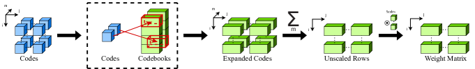
Figure 3: AQLM compressed weight format. Horizontal and vertical axes are input features and output units, respectively. Depth represents the codebook index. Reconstruction procedure, from left to right: i) compressed weight codes ii) zoom-in one weight group, each code is an index in its respective codebook iii) select codes from each codebook iv) add up codes as in (2) v) multiply by scales (one scale per output dimension).

Prior work addresses this issue via quantization-aware training (QAT), e.g. (Gholami et al., 2021). Instead of compressing the entire model in a single pass, they quantize model parameters gradually and train the remaining parameters to compensate for the quantization error. Unfortunately, running QAT in our setting is infeasible, since most modern LLMs are extremely expensive to train or even fine-tune. Thus, most PTQ algorithms for LLMs only adjust model parameters within the same linear layer (Frantar et al., 2022a; Lin et al., 2023; Dettmers et al., 2023b).

Algorithm 1 AQLM: Additive Quantization for LLMs

0:  model, data

1:  $\mathbf{X}_{block}:=\texttt{model.input\_embeddings(data)}$

2:  for $i=1,\dots,\texttt{model.num\_layers}$ do

3:    block := model.get_block(i)

4:    $\mathbf{Y}_{block}:=\texttt{block}(\mathbf{X}_{block})$

5:    for $\texttt{layer}\in\texttt{linear\_layers(block)}$ do

6:       $\mathbf{W}:=\texttt{layer.weight}$

7:       $\mathbf{X}:=\texttt{layer\_inputs}(\texttt{layer},\mathbf{X}_{block})$

8:       $C,b,s:=\texttt{initialize}(\mathbf{W})$ // k-means

9:       while  loss improves by at least $\tau$ do

10:          $C,s:=\texttt{train\_Cs\_adam}(\mathbf{XX}^{T},\mathbf{W},C,b,s)$

11:          $b:=\texttt{beam\_search}(\mathbf{XX}^{T},\mathbf{W},C,b,s)$

12:       end while

13:       /* save for fine-tuning */

14:       $\texttt{layer.weight}:=\texttt{AQLMFormat}(C,b,s)$

15:    end for

16:    $\theta:=\texttt{trainable\_parameters}(\texttt{block})$

17:    while  loss improves by at least $\tau$ do

18:       $L:=||\texttt{block}(\mathbf{X}_{block})-\mathbf{Y}_{block}||_{2}^{2}$

19:       $\theta:=\texttt{adam}(\theta,\frac{\partial{L}}{\partial{\theta}})$

20:    end while

21:    $\mathbf{Y}_{block}:=\texttt{block}(\mathbf{X}_{block})$

22:  end for

Here, we opt for a middle ground by performing optimization at the level of individual transformer blocks, i.e. groups of 4-8 linear layers that constitute a single multi-head self-attention, followed by a single and MLP layer. Having quantized all linear layers within a single transformer block, we fine-tune its remaining parameters to better approximate the original outputs of that transformer block by backpropagating through the weight representation (2).

Concretely, we use the PyTorch autograd engine to differentiate the $||\text{block}(\mathbf{X}_{block})-\mathbf{Y}_{block}||^{2}$ , where $\mathbf{X}_{block}$ are the inputs activations for that transformer block and $\mathbf{Y}_{block}$ are output activations of $\text{block}(\mathbf{X}_{block})$ recorded prior to quantization. We train the codebooks $C_{m}$, scale vectors $s$ and all non-quantized parameters (RMSNorm scales and biases), while keeping the codes $b_{i,j,m}$ frozen. Similarly to Section 3.3, we train these parameters using Adam to minimize the MSE against the original block outputs (prior to quantization). This phase uses the same calibration data as for the individual layer quantization. The full procedure is summarized in Alg. 1.

While fine-tuning blocks is more expensive than individual linear layers, it is still possible to quantize billion-parameter models on a single GPU in reasonable time. Also, since the algorithm only modifies a few trainable parameters, it uses little VRAM for optimizer states. This fine-tuning converges after a few iterations, as it starts from a good initial guess. In practice, fine-tuning transformer layers takes a minority (10-30% or less) of the total calibration time.

Table 1: Evaluation of quantized Llama 2 models for 2-2.8 bits per parameter, with an extra section for higher bitwidth. We report perplexity on WikiText2 (Merity et al., 2016) & C4 (Raffel et al., 2020) and accuracy for zero-shot tasks. The Average accuracy is the mean of 5 zero-shot tasks. Primary metrics are Wiki2 (PPL), C4 (PPL) and Average accuracy.

Size	Method	Avg bits	Wiki2$\downarrow$	C4$\downarrow$	WinoGrande$\uparrow$	PiQA$\uparrow$	HellaSwag$\uparrow$	ArcE$\uparrow$	ArcC$\uparrow$	Average accuracy$\uparrow$
7B	–	16	5.12	6.63	67.25	78.45	56.69	69.32	40.02	62.35
	AQLM	2.02	6.64	8.56	64.17	73.56	49.49	61.87	33.28	56.47
	QuIP#	2.02	8.22	11.01	62.43	71.38	42.94	55.56	28.84	52.23
	AQLM	2.29	6.29	8.11	65.67	74.92	50.88	66.50	34.90	58.57
13B	–	16	4.57	6.05	69.61	78.73	59.72	73.27	45.56	65.38
	AQLM	1.97	5.65	7.51	65.43	76.22	53.74	69.78	37.8	60.59
	QuIP	2.00	13.48	16.16	52.80	62.02	35.80	45.24	23.46	43.86
	QuIP#	2.01	6.06	8.07	63.38	74.76	51.58	64.06	33.96	57.55
	AQLM	2.18	5.41	7.20	68.43	76.22	54.68	69.15	39.42	61.58
	AQLM	2.53	5.15	6.80	68.11	76.99	56.54	71.38	40.53	62.71
	AQLM	2.76	4.94	6.54	68.98	77.58	57.71	72.90	43.60	64.15
70B	–	16	3.12	4.97	76.95	81.07	63.99	77.74	51.11	70.17
	AQLM	2.07	3.94	5.72	75.93	80.43	61.79	77.68	47.93	68.75
	QuIP	2.01	5.90	8.17	67.48	74.76	50.45	62.16	33.96	57.76
	QuIP#	2.01	4.16	6.01	74.11	79.76	60.01	76.85	47.61	67.67

Table 2: Evaluation of quantized Llama 2 models for 3-3.1 bits per parameter, with the same metrics as in Table 1.

Size	Method	Avg bits	Wiki2$\downarrow$	C4$\downarrow$	WinoGrande$\uparrow$	PiQA$\uparrow$	HellaSwag$\uparrow$	ArcE$\uparrow$	ArcC$\uparrow$	Average accuracy$\uparrow$
7B	–	16	5.12	6.63	67.25	78.45	56.69	69.32	40.02	62.35
	AQLM	3.04	5.46	7.08	66.93	76.88	54.12	68.06	38.40	60.88
	GPTQ	3.00	8.06	10.61	59.19	71.49	45.21	58.46	31.06	53.08
	SpQR	2.98	6.20	8.20	63.54	74.81	51.85	67.42	37.71	59.07
13B	–	16	4.57	6.05	69.61	78.73	59.72	73.27	45.56	65.38
	AQLM	3.03	4.82	6.37	68.43	77.26	58.30	70.88	42.58	64.49
	GPTQ	3.00	5.85	7.86	63.93	76.50	53.47	65.66	38.48	59.61
	SpQR	2.98	5.28	7.06	67.48	77.20	56.34	69.78	39.16	61.99
	QuIP	3.00	5.12	6.79	69.93	76.88	57.07	70.41	41.47	63.15
70B	–	16	3.12	4.97	76.95	81.07	63.99	77.74	51.11	70.17
	AQLM	3.01	3.36	5.17	77.19	81.28	63.23	77.61	50.00	69.86
	GPTQ	3.00	4.40	6.26	71.82	78.40	60.00	72.73	44.11	65.41
	SpQR	2.98	3.85	5.63	74.66	80.52	61.95	75.93	48.04	68.22
	QuIP	3.01	3.87	5.67	74.59	79.98	60.73	73.19	46.33	66.96

4 Experiments

We evaluate the AQLM algorithm in typical scenarios for post-training quantization of modern LLMs. Our evaluation is focused on the Llama 2 model family since it is a popular backbone for fine-tuned models or general LLM applications, e.g. (Dettmers et al., 2023a), and we also present results on Mistral-family models (Jiang et al., 2024). In Section 4.1, we evaluate the full AQ procedure for various Llama 2 models and quantization bit-widths; Section 4.2 presents an ablation analysis for individual AQ components and implementation details.

4.1 Compression quality for modern LLMs

We report perplexity on WikiText2 (Merity et al., 2016) and C4 (Raffel et al., 2020) validation sets. We also measure zero-shot accuracy on WinoGrande (Sakaguchi et al., 2021), PiQA (Tata & Patel, 2003), HellaSwag (Zellers et al., 2019), ARC-easy and ARC-challenge (Clark et al., 2018) via the LM Eval Harness (Gao et al., 2021). We broadly follow the evaluation setup of GPTQ (Frantar et al., 2022a).

We consider three main targets in terms of compression ranges: 2-2.8 bits, 3-3.1 bits, and 4-4.1 bits per model parameter. In the results below average bits per parameter takes into account only quantized weights, we do not include parameters kept in floating precision similarly to the related work. The details on the model size estimate are provided in Appendix G. We compare AQ against GPTQ for 3&4 bits (Frantar et al., 2022a), SpQR for 3&4 bits (Dettmers et al., 2023b), QuIP in 2,3 & 4 bits (Chee et al., 2023) and QuIP# for 2&4 bits (Tseng et al., 2023). While GPTQ and SpQR technically support 2-bit quantization, they perform poorly in the 2-3 bit range. For QuIP, we omit results for the 7B model, as we could not achieve competitive performance in this one scenario using the available implementations. (Currently, there is no official implementation of the original QuIP (non-#) for the Llama 2 model.) For QuIP#, we focus on 2 and 4 bit because the available implementation does not yet support 3-bit compression. We calibrate each algorithm using the subset of RedPajama dataset (Computer, 2023), with a sequence length of 4096.

The exact bit-widths for each method are dictated by parameters such as the number of codebooks and code width. We report results for the $2{-}2.8$ and $3{-}3.1$ bitwidth ranges in Tables 1 and 2, respectively. Additional results for $4-4.1$ bits are deferred to Appendix E.2.

The results show that AQLM outperforms the previous best PTQ algorithms across all settings, often by wide margins, especially at high compression. This holds both in terms of PPL across standard validation sets (Wiki-Text2 and C4), and accuracy across zero-shot tasks. Specifically, we observe the highest accuracy gains in the “extreme” 2-2.1 bits per parameter range, where the deviation from the uncompressed model becomes large for all methods.

Table 3: Evaluation of quantized Mixtral (Jiang et al., 2024) models for 2 bits. The table reports perplexity on WikiText2 (Merity et al., 2016) and C4 (Raffel et al., 2020), as well as accuracy for zero-shot tasks. The Average accuracy column is the mean of 5 zero-shot task accuracies. Primary metrics are Wiki2 (PPL), C4 (PPL) and Average accuracy.

Size	Method	Avg bits	Wiki2$\downarrow$	C4$\downarrow$	WinoGrande$\uparrow$	PiQA$\uparrow$	HellaSwag$\uparrow$	ArcE$\uparrow$	ArcC$\uparrow$	Average accuracy$\uparrow$
8x7B	–	16	3.46	5.02	75.45	82.37	64.65	83.38	55.80	72.33
	AQLM	1.98	4.61	5.75	73.64	79.27	57.91	78.96	48.63	67.68
	QuIP#	2.01	4.75	5.89	71.11	79.05	58.23	77.57	45.73	66.34

Mixtral quantization.

Table 3 presents results on the Mixtral MoE-type model, comparing against QuIP# at 2-bits. (See Appendix E.1 for full results.) AQLM outperforms QuIP# in this case as well. Although the margins are lower compared to Llama 2 models, they are still significant for “harder” tasks, such as Arc Challenge (+3 points).

Pareto optimality of AQLM. The significant error improvements raise the question of choosing the “optimal” model variant to maximize accuracy within a certain memory budget. For this, we follow Dettmers & Zettlemoyer (2022): a quantized model is said to be Pareto-optimal if it maximizes accuracy at the same or lower total size (bytes). Despite rapid progress, prior art methods are not Pareto-optimal at 2-bits: for instance, the previous best 2-bit Llama 2 13B (QuIP#, Table 1) achieves Wiki2 PPL of 6.06, but one can get much lower 5.21 PPL by using a 7B model with 4-bit quantization, which is smaller (see Appendix Table 10).

AQLM compression to strictly 2 bits for the same model is also below Pareto-optimality, as it is outperformed by 4-bit AQLM compression for Llama 2 7B (5.21 vs 5.65). To find the Pareto-optimal quantization bitwidth, we run experiments between 2-3 bits per parameter and report them in Table 1, below horizontal bars. Thus, the Pareto-optimal bitwidth for AQLM appears to be around 2.5 bits per parameter (Table 1), at which point we are comparable to 5-bit AQLM for Llama 2 7B (Appendix Table 10). In turn, the 2.76-bit AQLM on 13B outperforms the uncompressed 7B model. As such, AQLM is the first algorithm to achieve Pareto-optimality at less than 3 bits per parameter.

4.2 Ablation analysis

In Appendix D, we examine key design choices regarding initialization, alternating optimization, the impact of the fine-tuning protocol, distribution of codebooks vs groups, as well as other hyper-parameters. In brief, we first find that the residual K-means initialization is critical for fast algorithm convergence: when compared with random initialization, it needs significantly fewer training iterations. Second, to validate our calibration fine-tuning procedure, we compare it against 1) no fine-tuning, 2) fine-tuning only of non-linear layers (e.g. RMSNorm) but not of codebook parameters, and 3) fine-tuning only the codebooks (but not other layers). The results, presented in full in Appendix D, show that fine-tuning the codebook parameters has the highest impact on accuracy, by far, while fine-tuning the RMSNorm only has minor impact. This validates our choice of leveraging the calibration set for learned codebooks.

Further, we observe that increasing the number of sample sequences in the range 128 to 4096 leads to a gradual PPL improvement, but with diminishing returns. In this respect, AQLM benefits more from larger calibration sets (similarly to QuIP#), as opposed to direct methods like GPTQ which saturate accuracy at around 256 input sequences. Finally, we investigate various options for investing a given bit budget, comparing e.g. longer codes (e.g. 1x15) vs multiple codebooks with shorter codes (e.g. 2x8).

4.3 Inference Speed

Although our primary objective is to maximize accuracy for a given model size, AQLM can also be practical in terms of inference latency. To demonstrate this, we implemented efficient GPU and CPU kernels for a few hardware-friendly configurations of AQLM. The results can be found in Table 4. For GPU inference, we targeted quantized Llama 2 models with 16-bit codebooks, corresponding to 2.07 bits for Llama 2 70B, 2.18 bits for 13B, and 2.29 bits for 7B models (see Table 1), as well as a 2x8-bit codebook model with perplexity 7.98 on Wiki2. For each model we benchmark the matrix-vector multiplication subroutine performance on a standard layer. The results show that AQLM can execute at speeds comparable to or better than FP16. End-to-end generative numbers on a preliminary HuggingFace integration can be found in Appendix H: for instance, we can achieve $\sim$ 6 tokens/s on Llama 2 70B in this setting. We observe that multiple smaller codebooks allow efficient GPU cache utilization, leading to greater speedup, at the price of slightly lower accuracy.

Table 4: Speed of the FP16 gate_proj layer matrix-vector multiplication in PyTorch, and relative AQLM speedups.

Llama 2	7B	13B	70B
2 bit speedup over FP16 on Nvidia RTX 3090 GPU
Original (float16)	129 $\mu$s	190 $\mu$s	578 $\mu$s
AQLM (Table 1)	x1.31	x1.20	x1.20
AQLM ($2\times$8-bit)	x1.57	x1.82	x3.05
2 bit speedup over FP32 on Intel i9 CPU, 8 cores
Original (float32)	1.83 ms	3.12 ms	11.31 ms
AQLM ($2\times$8-bit)	x2.75	x3.54	x3.69
AQLM ($4\times$8-bit)	x2.55	x3.02	x4.07
AQLM ($8\times$8-bit)	x2.29	x2.68	x4.03

Next, we explore how to leverage AQLM to accelerate CPU inference. As discussed in Section 2.2, additive quantization can compute dot products efficiently if the codebook size is small. One way to achieve it for AQLM is to replace each 16-bit codebook with a number of smaller 8-bit ones. This leads to higher quantization error, but still outperforms the baselines in terms of accuracy (see Appendix Table 9). The results in Table 4 show that this also allows for up to 4x faster inference relative to FP32 on CPU.

5 Conclusion and Future Work

We presented AQLM, a new form of additive quantization (AQ) targeted to LLM compression, which significantly improved the state-of-the-art results for LLM quantization in the regime of 2 and 3 bits per weight. In terms of limitations, AQLM is more computationally-expensive than direct post-training quantization methods, such as RTN or GPTQ, specifically because of the use of a more complex coding representation. Yet, despite the more sophisticated encoding and decoding, we have shown AQLM lends itself to efficient implementation on both CPU and GPU. Overall, we find it remarkable that, using AQLM, massive LLMs can be executed accurately and efficiently using little memory.

6 Acknowledgements

Authors would like to thank Ruslan Svirschevski for his help in solving technical issues with AQLM and baselines. We also thank Tim Dettmers for helpful discussions on the structure of weights in modern LLMs and size-accuracy trade-offs.The authors would also like to thank Daniil Pavlov for his assistance with CPU benchmarking. Finally, authors would like to thank the communities of ML enthusiasts known as LocalLLaMA and Petals community on discord for the crowd wisdom about running LLMs on consumer devices.

Appendix A Full model fine-tuning

The block-wise finetuning procedure, introduced in 3.4, considerably improves performance of compressed models. However, block-wise finetuning optimizes the loss only at the level of a current transformer block and is agnostic of the actual task of interest. To minimize the target loss, one can run backpropagation through the whole model and optimize all trainable parameters to directly optimize the end objective.

This allows to search for globally optimal parameters, as opposed to sequentially selected ones, during block-wise finetuning.

One can minimize the error between the quantized model and the floating-point model on some calibration set. The parameters being optimized (namely the codebooks, scales and the non-quantized parameters) typically constitute a small fraction of the total number of parameters in the original model. Therefore, the proposed distillation method is an instance of parameter-efficient finetuning.

Standard Knowledge distillation (Hinton et al., 2015) optimizes the KL-divergence between the outputs of teacher and student models. However, according to the literature, (Sun et al., 2019; Kurtic et al., 2023) transfer of intermediate representation facilitates faster convergence and enhances performance. Hence, we decided to perform knowledge transfer between some intermediate activations in addition to the model output. Specifically, we take a subset of transformer blocks $\{l_{0},l_{1}\ldots,l_{K-1}\},l_{i}\in[0,L-1]$, where $L$ is the number of transformers block in the model, and optimize the following objective:

$$\sum_{i=0}^{K-1}\mathcal{L}(x_{l_{i}}^{(s)},x_{l_{i}}^{(t)})$$ (9)

Where $x_{l_{i}}^{(s)}$ and $x_{l_{i}}^{(t)}$ are the student and teacher output activations respectively at block $l_{i}$ and $\mathcal{L}(*,*)$ is some loss function. We considered the following options:

• $L_{2}$ loss: $\|x-y\|_{2}^{2}$

• Normalized $L_{2}$ loss: $\|x-y\|_{2}^{2}/\|y\|_{2}^{2}$

• Cosine distance: $\frac{1}{2}\left(1-\frac{(x,y)}{\|x\|\|y\|}\right)$

We tune all models for a single epoch on the same calibration set used for additive quantization and block finetuning. We observe that longer training leads to overfitting. Learning rate of $\eta=1e-5$ and batch size of $32$ with Adam optimizer are used in full model finetuning experiments. We find that simple $L_{2}$ loss outperforms the alternatives (Table 5), and that the number of intermediate activations used in the loss function barely affects the final performance (Table 6).

Table 5: Ablation on the choice of loss for Knowledge distillation.

Loss	Wiki2$\downarrow$	C4$\downarrow$
$L_{2}$	$\mathbf{6.57}$	$\mathbf{8.48}$
Normalized $L_{2}$	6.63	8.57
Cosine distance	6.65	8.59

Table 6: Ablation on the choice of blocks subset for Knowledge distillation. Empty set means no knowledge distillation applied.

Blocks	Wiki2$\downarrow$	C4$\downarrow$
$\{\}$	6.64	8.56
$\{31\}$	$\mathbf{6.52}$	8.51
$\{15,31\}$	6.57	$\mathbf{8.48}$
$\{7,15,23,31\}$	6.55	8.49
$\{3,7,11,15,19,23,27,31\}$	6.57	8.54

Overall, the improvement due to knowledge distillation is not very significant while increasing the complexity of the quantization pipeline, therefore, we decided to not include KD in our main setup.

Appendix B Code reproducibility

We share the code for our method in the GitHub repository https://github.com/vahe1994/AQLM. The hyperparameters for our experimental setup are discussed in Appendix C.

Appendix C Experimental Configurations

Hardware. In all of our experiments, we used either Nvidia A100 or H100. The number of GPUs varied from 1 to 8. We used activation offloading to lower pick memory usage. To evaluate inference speed on GPU we used consumer-grade GPU Nvidia 3090 and for CPU setup we used Intel core i9 13900k.

Calibration set. All methods were calibrated on a slice of RedPajama-v1 dataset (Computer, 2023) for both Llama and Mistral/Mixtral family models. We used the same context length as models were trained on, for Llama-2 4096 and for Mistral/Mixtral 8192.

For Llama-2 experiments, we used 8M tokens as a calibration set for SpQR, GPTQ, and AQLM. Quip, however, was calibrated on 4M tokens due to OOM errors when trying to use more samples. Taking into account the fact that after 2M tokens improvement of methods results is fairly small we chose to report these numbers as is. For Quip#, we used Llama-2 and Mistral’s quantized models provided by authors in their GitHub repository. To the best of our knowledge, they used 6k samples for calibration with a context length of 4096/8192.
For Mixtral we calibrated both our method and QUIP# on 8M tokens with context length 8192.

Hyperparameters.

For GPTQ for both 3 and 4 bits we used a standard set of parameters without grouping and with permutation order act_order.

SpQR method was evaluated with base 2 and 3 bit-width with group size of 16 and 3 bits for zeros and scales. Outliers rate was chosen such that average bit will be close to 3 and 4 bits respectively.

Quip was adapted to work on the Llama family and was calibrated with 1024 samples and 4096 context length.

Quip# For Llama-2 and Mistral models we used the officially published quantized models. For Mixtral we adapted the code to work with the model’s architecture and quantized it with the recommended set of parameters. For both AQLM and QuIP#, we don’t quantize gate linear layer in Mixtral, because it contains relatively small amount of paramters and have severe impact on performance.

AQLM For to get 2, 3, 4 bits: we used 1 codebook size of $2^{15}$ or $2^{16}$, with groups of 8 for 2 bits. For 3 bits we used 2 codebooks size of $2^{12}$ with groups of 8. Finally for 4 bits we used 2 codebooks size of $2^{15}$ or $2^{16}$ with groups of 8.

Both for finetuning 3.4 and codebooks update 3.3 we used Adam optimizer (Kingma & Ba, 2015) with learning rate of $10^{-4}$, $\beta_{1}=0.90$ and $\beta_{2}=0.95$. We used early stopping both for the finetuning phase and for the codebook optimization phase, by stopping when the least square error not decreasing more than some threshold. In our experiments the threshold varies between $10^{-2}$ and $10^{-3}$.

Appendix D Ablation analysis

The AQLM algorithm makes several design choices that need to be validated separately: initialization, alternating optimization, the fine-tuning protocol, and the choice of hyperparameters. Here, we study how each of these components affect results.

Initialization. As discussed in Section 3, we initialize AQLM with residual K-means to obtain a good initial guess for both codes and codebooks. That is, we run K-means for the weight matrix, then subtract the nearest cluster from each weight, and run K-means again M times. A simple baseline would be to initialize all codes uniformly at random. We compare the two initialization strategies for the problem of quantizing a single linear layer within Llama 2 70B model to 3 bits per parameter. We quantize groups of 8 consecutive weights using 2 codebooks, 12 bit each. Each codebook contains ${2^{12}}$ learnable values. As we can see in Figure 4, AQLM with K-means initialization needs significantly fewer training iterations to achieve the desired loss. The difference is so drastic that we expect that running AQLM with a random initialization would require extremely high runtimes to accurately quantize the largest models.

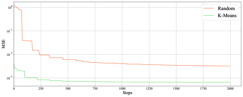
Figure 4: MSE loss learning curves of AQLM trained on the self attention q_proj linear layer of 10-th block in the Llama 2 70B model.

Fine-tuning. Next, we validate the fine-tuning procedure. We compare the full block fine-tuning (default) against three alternatives: i) no fine-tuning at all, ii) fine-tuning only non-linear layers (i.e. RMSNorm), but not the AQ parameters, and iii) fine-tuning only the AQ parameters, but not the non-linear layers. Table 7 summarizes our results: fine-tuning the entire model or only AQ parameters achieves competitive performance, while training only RMSNorm scales is comparable to not fine-tuning at all. We attribute these observations to the fact that over 99% of quantized layer parameters are contained in AQ codebooks $C_{m}$, whereas the remaining parameters are small 1-dimensional tensors. This validates the use of the AQ approach, as many competing algorithms do not have learnable per-layer codebooks. Notably, QuIP# uses a shared fixed lattice instead. We also note that, even without fine-tuning, AQLM is competitive to previous state-of-the-art results.

Table 7: Ablation analysis of AQLM with different fine-tuning restrictions on Llama-2 7B model at 2.02 bit width.

Name	Wiki2$\downarrow$	C4$\downarrow$
w/o	8.18	10.59
RMSnorm	8.31	10.46
AQ params	6.92	8.85
Full	6.93	8.84

Number of samples. We verify our choice of calibration hyperparameters. Traditionally, most PTQ algorithms use several hundred calibration sequences (e.g. Frantar et al. (2022a) has 128). In our experiments, we evaluate both AQLM and baselines with additional calibration data. Our original motivation for that was to avoid potential overfitting when fine-tuning entire transformer blocks. To test this assumption, we run our algorithm with different calibration set sizes, varying from 128 to 4096 sequences. For each size, we report the average perplexity on WikiText2 over 3 runs, along with standard deviations. The results in Table 8 demonstrate that increasing the number of samples leads to gradual reduction in perplexity with seemingly diminishing returns. Since the perplexity is still monotonically improving from 128 to 4096 samples, it is possible that larger sample sizes would yield further improvements.

Number of codebooks vs groups. Finally, we conducted an additional set of experiments on LLama-2 7B models to see perplexity dependence on simultaneous change of both codebooks and groups keeping compression rate fixed to 2bits. 9

We can see that the simultaneous increase in both the number of codebooks and groups led to a decrease in average perplexity and stopped when the number of groups reached 64.

Table 8: Wikitext2 PPL as a function of calibration set size for Llama 2 (7B) quantized to 2.3 bits with AQLM, averaged over 3 runs. SD stands for adjusted standard deviation.

# of samples	Average PPL	SD
128	6.994	0.127
256	6.584	0.031
512	6.455	0.005
1024	6.353	0.008
2048	6.297	0.018
4096	6.267	0.005

Table 9: Wikitext2 PPL as a function of from groups and number of codebook for Llama 2 (7B) quantized with approximately 2 bits quantization.

# of codebooks	Groups size	Average PPL
1	4	41.79
2	8	11.96
4	16	8.53
8	32	7.83
15	64	7.86

Appendix E Additional experiments

In this section we report additional experimental results for Mixtral(Jiang et al., 2024) , Mistral7B(Jiang et al., 2023) and LLama-2 model.

Table 10: Evaluation of quantized Llama 2 models for 4+ bits per parameter. The table reports perplexity on WikiText2 (Merity et al., 2016) and C4 (Raffel et al., 2020), as well as accuracy for zero-shot tasks. The Average accuracy column is the mean of 5 zero-shot task accuracies. Primary metrics are Wiki2 (PPL), C4 (PPL) and Average accuracy.

Size	Method	Avg bits	Wiki2$\downarrow$	C4$\downarrow$	WinoGrande$\uparrow$	PiQA$\uparrow$	HellaSwag$\uparrow$	ArcE$\uparrow$	ArcC$\uparrow$	Average accuracy$\uparrow$
7B	–	16	5.12	6.63	67.25	78.45	56.69	69.32	40.02	62.35
	AQLM	4.04	5.21	6.75	67.32	78.24	55.99	70.16	41.04	62.55
	GPTQ	4.00	5.49	7.20	68.19	76.61	55.44	66.20	36.77	60.64
	SpQR	3.98	5.28	6.87	66.93	78.35	56.10	69.11	39.68	62.17
	QuIP#	4.02	5.29	6.86	66.85	77.91	55.78	68.06	39.68	61.66
	AQLM	5.02	5.16	6.68	67.40	78.29	56.53	68.94	39.93	62.22
13B	–	16	4.57	6.05	69.61	78.73	59.72	73.27	45.56	65.38
	AQLM	3.94	4.65	6.14	69.85	78.35	59.27	73.32	44.80	65.12
	GPTQ	4	4.78	6.34	70.01	77.75	58.67	70.45	42.49	63.87
	SpQR	3.98	4.69	6.20	69.69	78.45	59.25	71.21	44.52	64.42
	QuIP	4.00	4.76	6.29	69.69	79.00	58.91	73.27	44.88	65.15
	QuIP#	4.01	4.68	6.20	69.38	77.91	58.86	73.74	44.63	64.90
70B	–	16	3.12	4.97	76.95	81.07	63.99	77.74	51.11	70.17
	AQLM	4.14	3.19	5.03	76.48	81.50	63.69	77.31	50.68	69.93
	GPTQ	4.00	3.35	5.15	75.61	81.23	63.47	76.81	49.15	69.25
	SpQR	3.97	3.25	5.07	76.01	81.28	63.71	77.36	49.15	69.50
	QuIP	4.00	3.58	5.38	76.01	80.25	61.97	74.28	47.01	67.90
	QuIP#	4.01	3.22	5.05	76.80	81.45	63.51	78.37	50.85	70.20
	AQLM	3.82	3.21	5.03	76.32	80.90	63.69	77.61	50.34	69.77

E.1 Mixtral

We report the results for Mixtral(Jiang et al., 2024) MoE-type model for 3 and 4 bits in Table 11. In the 4 bit case, performance of QuIP# and AQLM are very similar across all metrics and close to uncompressed FP16 model.

Table 11: Evaluation of quantized Mixtral (Jiang et al., 2024) models for 3 and 4 bits per parameter. The table reports perplexity on WikiText2 (Merity et al., 2016) and C4 (Raffel et al., 2020), as well as accuracy for zero-shot tasks. The Average accuracy column is the mean of 5 zero-shot task accuracies. Primary metrics are Wiki2 (PPL), C4 (PPL) and Average accuracy.

Size	Method	Avg bits	Wiki2$\downarrow$	C4$\downarrow$	WinoGrande$\uparrow$	PiQA$\uparrow$	HellaSwag$\uparrow$	ArcE$\uparrow$	ArcC$\uparrow$	Average accuracy$\uparrow$
3-bit	–	16.00	3.46	5.02	75.45	82.37	64.65	83.38	55.80	72.33
	AQLM	3.02	3.8	5.18	74.74	81.77	63.22	82.28	52.30	70.86
4-bit	–	16.00	3.46	5.02	75.45	82.37	64.65	83.38	55.80	72.33
	AQLM	3.915	3.57	5.07	74.82	81.99	64.23	83.12	54.61	71.75
	QuIP#	4.000	3.60	5.08	76.56	81.99	63.92	82.62	54.78	71.97

E.2 Llama-2

We show results for 4 bit quantization of the Llama 2 models in Table 10. We can see that AQLM outperforms other methods in terms of perplexity and has the best or close to the best results. We also report results of perplexity for our quantized 2x8 codebooks models in Table 12.

Table 12: Wikitext2 and C4 PPL for quantized Llama 2 models for 2x8 codebooks models.

Name	Wiki2$\downarrow$	C4$\downarrow$
7B	7.98	10.38
70B	4.83	6.66

Table 13: Evaluation of quantized Mistral7B (Jiang et al., 2023) models for 2, 3 and 4 bits per parameter: perplexity on WikiText2 (Merity et al., 2016) and C4 (Raffel et al., 2020), as well as accuracy for zero-shot tasks. The Average accuracy column is the mean of 5 zero-shot task accuracies. Primary metrics are Wiki2 (PPL), C4 (PPL) and Average accuracy.

Size	Method	Avg bits	Wiki2$\downarrow$	C4$\downarrow$	WinoGrande$\uparrow$	PiQA$\uparrow$	HellaSwag$\uparrow$	ArcE$\uparrow$	ArcC$\uparrow$	Average accuracy$\uparrow$
2-bit	–	16.00	4.77	5.71	73.64	80.47	61.15	78.87	49.23	68.67
	AQLM	2.01	6.32	6.93	68.75	76.01	52.13	73.65	40.44	62.17
	QuIP#	2.01	6.02	6.84	69.30	76.71	52.95	72.14	39.76	62.20
3-bit	–	16.00	4.77	5.71	73.64	80.47	61.15	78.87	49.23	68.67
	AQLM	3.04	5.07	5.97	72.69	80.14	59.31	77.61	46.67	67.28
4-bit	–	16.00	4.77	5.71	73.64	80.47	61.15	78.87	49.23	68.67
	AQLM	4.02	4.89	5.81	73.80	79.71	60.27	77.86	48.21	67.97
	QuIP#	4.01	4.85	5.79	73.95	80.41	60.62	78.96	49.40	68.67

E.3 Mistral

Finally we evaluate AQLM and QuIP# quantization on Mistral7b (Jiang et al., 2023) model for 3 and 4 bits in Table 13. In 2bits, QuIP# slightly outperform AQLM on most benchmarks. And for 4bits setup results are very close across the board.

Appendix F Pareto optimality

We visualize WikiText perplexity of Llama-2 7B,13B,70B models quantized with AQLM and QuIP# as plotted against quantized weight size in bytes and report it in Figure 5. Our method outperforms QuIP# in terms of perplexity in WikiText2 across all model sizes.

Additionally, in Figure 6, we show perplexity on WikiText for AQLM method against size of quantized parameters. We can notice that starting around 3.7 GiB of quantized weights, which correspond to 2.5 bits compression on Llama-2 13B model, it is more advantageous to compress 13B model rather 7B model at the same model size in bytes.

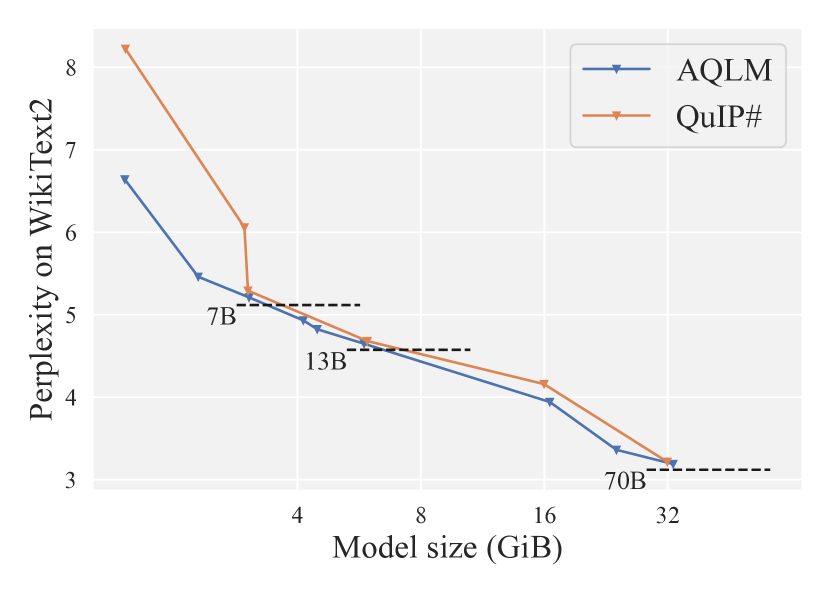
Figure 5: Comparison of AQLM relative to QuIP# on LLAMA-2 7B, 13B, and 70B models.

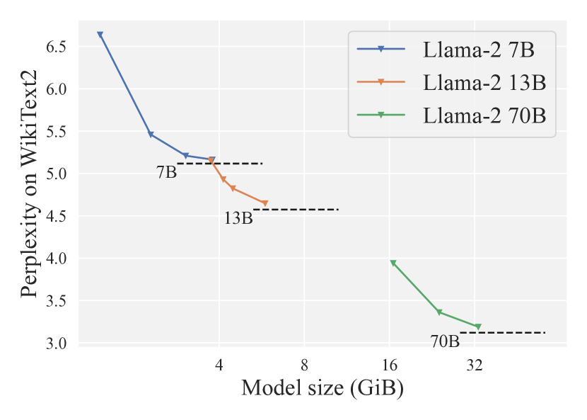
Figure 6: Model optimality for AQLM on LLAMA 2 7, 13, and 70B models.

Appendix G Estimating model size

In this section, we describe how to estimate the size of the quantized model for a given codebook configuration. The total cost of storing quantized weight comprises the codebooks, codes and per-unit scales. Specifically for a weight with input dimension $d_{in}$, output dimension $d_{out}$, group size $g$, $M$ codebooks corresponding to $B$-bit codes, the total amount of memory required is (assuming that codebooks and scales are stored in half precision):

• codebooks: $g\cdot M\cdot 2^{B}\cdot 16$

• codes: $d_{out}\cdot(d_{in}/g)\cdot B$

• scales: $d_{out}\cdot 16$

Therefore, the average bits per parameter can be computed as follows:

$$\bar{b}=\frac{\mathrm{size\ in\ bits}}{\mathrm{number\ of\ parameters}}=\frac{16\ g\ M\ 2^{B}+d_{out}\ (d_{in}/g)B+16\ d_{out}}{d_{out}d_{in}}$$ (10)

For example, for mlp.gate_proj layer of Llama 2 70B model with $d_{in}=8192$, $d_{out}=28672$, quantization with group size $8$, two $8$-bit codebooks the formula above yields $2.002$ bits per parameter. Typically, storage cost is dominated by the codes, whereas codebooks and scales induce small memory overhead.

Appendix H End-to-End Inference Speed

Table 14: Text generation speed benchmark.

Llama 2	7B	13B	70B
Inference on Nvidia RTX 3090 GPU, tok/s
Original (float16)	41.51	26.76	5.66
AQLM (Table 1)	32.22	25.04	5.65
AQLM ($2\times$8-bit)	32.64	25.35	6.03
Inference on Intel i9 CPU, 8 cores, tok/s
Original (float32)	3.106	1.596	0.297
AQLM ($2\times$8-bit)	6.961	4.180	0.966
AQLM ($4\times$8-bit)	6.837	4.004	0.948
AQLM ($8\times$8-bit)	5.319	3.193	0.775

For quantized Llama-2 models, the same setup as in Section 4.3, we measure the time it takes to generate 128 tokens from scratch with batch size 1, and report the average number of generated tokens per second on a single 24GB RTX 3090 GPU, as well as Intel i9 CPU, in Table 14.

Appendix I Codebook and codes distribution

The proposed AQLM quantization method allows for large freedom in the choice of quantization lattice and ability to represent different weight distribution. To understand how do the learned codes and codebooks look like, we visualize the distribution of codes (how frequently given codebook vector is chosen) and the learned codebooks. Below on Figure 7 we provide a histogram of leaned codes and two leading principal components for a specific layer. One can observe that codes are assigned uniformly across codebook vectors and codebook vectors are concentrated in some ball. This pattern is pertinent to all linear projections inside transformer blocks.

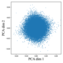
Figure 7: Visualization of learned codes and codebooks in layers.31.mlp.down_proj linear projection.
(Left) Codes distribution. (Right) Two leading principal components of codebook.

References

- Babenko & Lempitsky (2014) Babenko, A. and Lempitsky, V. Additive quantization for extreme vector compression. In Proceedings of the IEEE Conference on Computer Vision and Pattern Recognition, pp. 931–938, 2014.
- Besag (1986) Besag, J. On the statistical analysis of dirty pictures. Journal of the Royal Statistical Society Series B: Statistical Methodology, 48(3):259–279, 1986.
- Biderman et al. (2023) Biderman, S., Schoelkopf, H., Anthony, Q., Bradley, H., O’Brien, K., Hallahan, E., Khan, M. A., Purohit, S., Prashanth, U. S., Raff, E., et al. Pythia: A suite for analyzing large language models across training and scaling. arXiv preprint arXiv:2304.01373, 2023.
- Blalock & Guttag (2021) Blalock, D. and Guttag, J. Multiplying matrices without multiplying. In International Conference on Machine Learning, pp. 992–1004. PMLR, 2021.
- Burton et al. (1983) Burton, D., Shore, J., and Buck, J. A generalization of isolated word recognition using vector quantization. In ICASSP ’83. IEEE International Conference on Acoustics, Speech, and Signal Processing, volume 8, pp. 1021–1024, 1983. doi: 10.1109/ICASSP.1983.1171915.
- Chee et al. (2023) Chee, J., Cai, Y., Kuleshov, V., and Sa, C. D. Quip: 2-bit quantization of large language models with guarantees, 2023.
- Chen et al. (2019) Chen, S., Wang, W., and Pan, S. J. Deep neural network quantization via layer-wise optimization using limited training data. Proceedings of the AAAI Conference on Artificial Intelligence, 33(01):3329–3336, Jul. 2019. doi: 10.1609/aaai.v33i01.33013329. URL https://ojs.aaai.org/index.php/AAAI/article/view/4206.
- Chen et al. (2010) Chen, Y., Guan, T., and Wang, C. Approximate nearest neighbor search by residual vector quantization. Sensors, 10(12):11259–11273, 2010.
- Clark et al. (2018) Clark, P., Cowhey, I., Etzioni, O., Khot, T., Sabharwal, A., Schoenick, C., and Tafjord, O. Think you have solved question answering? try arc, the ai2 reasoning challenge. arXiv preprint arXiv:1803.05457, 2018.
- Computer (2023) Computer, T. Redpajama: an open dataset for training large language models, 2023. URL https://github.com/togethercomputer/RedPajama-Data.