Simulation-Based Inference with Neural Posterior Estimation applied to X-ray spectral fitting

Abstract

Context. Neural networks are being extensively used for modelling data, especially in the case where no likelihood can be formulated.

Aims. Although in the case of X-ray spectral fitting, the likelihood is known, we aim to investigate the neural networks ability to recover the model parameters but also their associated uncertainties, and compare its performance with standard X-ray spectral fitting, whether following a frequentist or Bayesian approach.

Methods. We apply Simulation-Based Inference with Neural Posterior Estimation (SBI-NPE) to X-ray spectra. We train a network with simulated spectra generated from a multi-parameter source emission model folded through an instrument response, so it learns the mapping between the simulated spectra and their parameters and returns the posterior distribution. The model parameters are sampled from a predefined prior distribution. To maximize the efficiency of the training of the neural network, yet limiting the size of the training sample to speed up the inference, we introduce a way to reduce the range of the priors, either through a classifier or a coarse and quick inference of one or multiple observations. For the sake of demonstrating working principles, we apply the technique to data generated from and recorded by the NICER X-ray instrument: a medium resolution X-ray spectrometer, covering the 0.2-12 keV band. We consider here simple X-ray emission models with up to 5 parameters.

Results. SBI-NPE is demonstrated to work equally well as standard X-ray spectral fitting, both in the Gaussian and Poisson regimes, both on simulated and real data, yielding fully consistent results in terms of best fit parameters and posterior distributions. The inference time is comparable to or smaller than the one needed for Bayesian inference, when involving the computation of large Markov Chain Monte Carlo chains to derive the posterior distributions. On the other hand, once properly trained, an amortized SBI-NPE network generates the posterior distributions in no time (less than 1 second per spectrum on a 6-core laptop). We show that SBI-NPE is less sensitive to local minima trapping than standard fit statistic minimization techniques. With a simple model, we find that the neural network can be trained equally well on dimension-reduced spectra, via a Principal Component Decomposition, leading to a faster inference time with no significant degradation of the posteriors.

Conclusions. We have shown that neural posterior estimation adds up as a complementary tool for X-ray spectral fitting. It is robust and produces well calibrated posterior distributions. It holds great potential for its integration in pipelines developed for processing large data sets. The code developed for this application, which is straightforward to use, will be made available through GitHub, once the paper has undergone its review process.

1 Introduction

X-ray spectral fitting relies generally on frequentist and Bayesian approaches (see Buchner & Boorman (2023) for a recent and comprehensive review on the statistical aspects of X-ray spectral analysis). Fitting of X-ray spectra with neural networks has been introduced by Ichinohe et al. (2018) for the analysis of high spectral resolution galaxy cluster spectra and recently by Parker et al. (2022) for the analysis of lower resolution Athena Wide Field Imager spectra of Active Galactic Nuclei. Parker et al. (2022) showed that neural networks delivered comparable accuracy to spectral fitting, while limiting the risk of outliers caused by the fit getting stuck into a local false minimum (the nightmare of anyone involved in X-ray spectral fitting), yet providing an improvement of around three orders of magnitude in speed, once the network had been properly trained. On the other hand, no error estimates on the spectral parameter were provided in the methods explored by Parker et al. (2022).

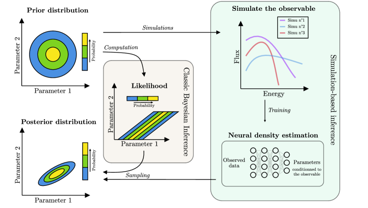
Figure 1: The Simulation-Based Inference approach emulates the traditional Bayesian inference approach. When assessing the parameters of a model, one first defines prior distributions, then defines the likelihood of a given observation, often using a forward-modelling approach. This likelihood is further sampled to obtain the posterior distribution of the parameters. The simulation-based approach does not require explicit computation of the likelihood, and instead will learn an approximation of the desired distribution (i.e. the likelihood or directly the posterior distribution) by training a neural network with a sample of simulated observations.

However, in a Bayesian framework, accessing the posterior distribution is possible through the Simulation-Based Inference with amortized Neural Posterior Estimation methodology (hereafter SBI-NPE, Papamakarios & Murray (2016); Lueckmann et al. (2017); Greenberg et al. (2019); Deistler et al. (2022)) (see Cranmer et al. (2020) for a review of simulation-based inference). In this approach, we sample parameters from a prior distribution and generate synthetic spectra from these parameters. Those spectra are then fed to a neural network that learns the association between simulated spectra and the model parameters. The trained network is then applied to data, to derive the parameter space consistent with the data and the prior, being the posterior distribution. In contrast to conventional Bayesian inference, SBI is also applicable when one can run model simulations, but no formula or algorithm exists for evaluating the probability of data given the parameters, i.e. the likelihood.

SBI-NPE has demonstrated its power in many fields, including astrophysics, e.g. to cite a few, for reconstructing galaxy spectra and inferring their physical parameters (Khullar et al., 2022), for inferring variability parameters from dead-time-affected light curves (Huppenkothen & Bachetti, 2022), for exoplanetary atmospheric retrieval (Vasist et al., 2023), for deciphering the ring down phase signal of the black hole merger GW150914 (Crisostomi et al., 2023) and very recently for isolated pulsar population synthesis (Graber et al., 2023).

In this paper, we demonstrate for the first time the power of SBI-SNPE for X-ray spectral fitting, to show that it delivers performances fully consistent with the XSPEC (Arnaud, 1996) and the Bayesian X-ray Analysis (BXA) spectral fitting packages (Buchner et al., 2014); two of the most commonly used tools for X-ray fitting. The paper is organised as follows. In Sec. 2, we give some more insights on the SBI-SNPE method. In Sec. 3, we present the methodology to produce the simulated data, introducing a method to reduce the prior range. In Sec. 4, we show examples of single round inference in the Gaussian and Poisson regimes for simulated mock data. In Sec. 5, we present a case based on multiple round inference. In Sec. 6, we demonstrate the robustness of the technique against local minima trapping. In Sec. 7, using a simple model, we apply the Principal Component Analysis to reduce the data fed to the network. In Sec. 8, we show the performance of SBI-NPE on real data, as recorded by the NICER X-ray instrument (Gendreau et al., 2012). In Sec. 9, we discuss the main results of the paper, listing some avenues for further investigations. This precedes a short conclusion.

2 SBI with amortized neural posteriors

2.1 Formalism

The SBI approach, illustrated in Fig. 1, aims at computing the probability distribution of interest, in this case the posterior distribution $p(\@vec{\theta}|\@vec{x})$, by learning an approximation of the probability density function from a joint sample of parameters $\left\{\@vec{\theta}_{i}\right\}$ and the associated simulated observables $\left\{\@vec{x}_{i}\right\}$, using neural density estimators such as normalizing flow. A normalizing flow $T$ is a diffeomorphism between two random variables, say $\@vec{X}$ and $\@vec{U}$, which links their following density functions as follows :

$$\@vec{X}=T(\@vec{U});\quad p_{\@vec{X}}(\vec{x})=p_{\@vec{U}}(\vec{u})\left|\text{det}\leavevmode\nobreak\ J_{T}(\vec{u})\right|^{-1}$$

where $J_{T}$ is the Jacobian matrix of the normalizing flow. The main idea when using normalizing flows is to define a transformation between a simple distribution (i.e. normal distribution) and the probability distribution that should be modelled, which eases the manipulation of such functions. To achieve this, an option is to compose several transformations $T_{i}$ to form the overall normalizing flow $T$, each parameterized using Masked Autoencoders for Density Estimation (MADE, Germain et al., 2015), which are based on deep neural networks. MADEs satisfy the autoregressive properties necessary to define a normalizing flow and can be trained to adjust to the desired probability density. Stacking several MADEs will form what is defined as a Masked Autoregressive Flow (MAF, Papamakarios et al., 2017). We refer interested readers to the following reviews by Papamakarios et al. (2021); Kobyzev et al. (2021). Greenberg et al. (2019) developed a methodology which enabled the use of MAFs to directly learn the posterior distribution of a Bayesian inference problem, using a finite set of parameters and associated observables $\left\{\@vec{\theta}_{i},\@vec{x}_{i}\right\}$. Using this approach, one can compute an approximation for the posterior distribution $q(\@vec{\theta},\@vec{x})\simeq p(\@vec{\theta}|\@vec{x})$, which can be used to obtain samples of spectral model parameters from the posterior distribution conditioned on an observed X-ray spectrum.

The python scripts from which the results presented here use the sbi package (Tejero-Cantero et al., 2020). sbi is a PyTorch-based package that implements SBI algorithms based on neural networks. It eases inference on black-box simulators by providing a unified interface to state-of-the-art algorithms together with very detailed documentation and tutorials. It is straightforward to use, involving the call of just a few Python functions.

Amortized inference enables the evaluation of the posterior for different observations without having to re-run inference. On the other hand, multi-round inference focuses on a particular observation. At each round, samples from the obtained posterior distribution computed at the observation are used to generate a new training set for the network, yielding in a better approximation of the true posterior at the observation. Although fewer simulations are needed, the major drawback is that the inference is no longer be amortized, being specific to an observation.

2.2 Benchmarking against the known likelihood

SBI implements machine learning techniques in situations where the likelihood is undefined, hampering the use of conventional statistical approaches. In our case, the likelihood is known. Here we recall the basic equations. Taking the notation of XSPEC (Arnaud, 1996), the likelihood of Poisson data (assuming no background) is known as :

$$L=\prod_{i=1}^{n}(tm_{i})^{S_{i}}e^{-tm_{i}}/S_{i}!$$ (1)

where $S_{i}$ are the observed counts in the bin $i$ as recorded by the instrument, $t$ the exposure time over which the data were accumulated, and $m_{i}$ the predicted count rates based on the current model and the response of the instrument folding in, its instrument efficiency, its spectral resolution, its spectral coverage… see (Buchner & Boorman, 2023) for details on the folding process. The associated negative log-likelihood, given in Cash (1979) and often referred to as the Cash-statistic, is:

$$C=2\sum_{i=1}^{N}(tm_{i})-S_{i}\ln{(tm_{i})}+\ln{(S_{i}!)}$$ (2)

The final term which depends exclusively on the data (and hence does not influence the best-fit parameters) is replaced by its Stirling’s approximation to give :

$$C=2\sum_{i=1}^{N}(tm_{i})-S_{i}+S_{i}(\ln{(S_{i})}-\ln{(tm_{i})})$$ (3)

This is what is used for the statistic C-stat option in XSPEC  the best fit model is the one that leads to the lowest C-stat. The default XSPEC minimization method uses the modified Levenberg-Marquardt algorithm based on the CURFIT routine from Bevington & Robinson (2003). In the following sections, we use XSPEC with and without Bayesian inference, and compute Markov Chain Monte Carlo (MCMC) chains to get the parameter probability distribution and to compute errors on the best fit parameters, as to enable a direct comparison with the posterior distributions derived from SBI-SNPE. By default, we use the Goodman-Weare algorithm (Goodman & Weare, 2010), with 8 walkers, a burn-in phase of 5000 and a length of 50000. The analysis was performed with the pyxspec wrapper of XSPEC v.12.13.1 (Arnaud, 1996).

In addition to XSPEC  we have used the Bayesian X-ray Analysis (BXA) software package (Buchner et al., 2014) for the validation of our results. Among many useful features, BXA connects XSPEC to the nested sampling algorithm as implemented in UltraNest (Buchner, 2021) for Bayesian Parameter Estimation. BXA finds the best fit, computes the associated error bars and marginal probability distributions, see Buchner & Boorman (2023) for a comprehensive tutorial on BXA.

We now introduce a method to restrict the prior range, with the objective of providing the network a training sample that is not too far from the targeted observation(s). This derives in part from the challenge, that for this work the generation of spectra, the inference, the generation of the posteriors should be performed on a MacBook Pro 2.9 GHz 6-Core Intel Core i9, within a reasonable amount of time.

Model 1: tbabs x powerlaw
$N_{\rm H}$	$[0.1,0.3]$	Uniform
Gamma	$[0.5,2.5]$	Uniform
NormPL	$[0.01,100]$	Uniform or Log Uniform
Model 2: tbabs x (powerlaw+bbodyrad)
$N_{\rm H}$	$[0.15,0.35]$	Uniform
Gamma	$[1.,3.]$	Uniform
NormPL	$0.01,10.]$	Uniform or Log Uniform
kTbb	$[0.3,3.]$	Uniform
NormBB	$[1.,100000.]$	Uniform or Log Uniform
Model 3: tbabs x (powerlaw+bbodyrad)
$N_{\rm H}$	$[0.2]$
Fixed Gamma	$[1.7]$
Fixed NormPL	$0.1,10.]$	Uniform or Log Uniform
kTbb	$[0.1,4.5]$	Uniform
NormBB	$[0.1,100000.]$	Uniform or Log Uniform

Table 1: Prior assumption for the emission models considered. The models are defined following the XSPEC convention. $N_{\rm H}$ is given in units of equivalent hydrogen column (in units of $10^{22}$ atoms cm^-2). Gamma is the power law photon index. NormPL is the power law normalisation at 1 keV in units of photons/keV/cm²/s. kTbb is the blackbody temperature in keV. NormBB is the blackbody normalisation given as $R_{km}^{2}/D_{10}^{2}$, where $R_{km}$ is the source radius in km and $D_{10}$ is the distance to the source in units of 10 kpc.

3 Generating an efficient training sample with a restricted prior

The density of the training sample depends on the range of the priors and the number of simulations. As the training time increases with the size of the training sample, ideally, one would like to train the network with a limited number of simulated spectra that are not too far from the targeted observation(s), yet covering plainly the observation(s). Here, we consider two methods to restrict the priors: one in which we train a network to retain the “good” samples of $\vec{\theta}_{i}$ matching a certain condition, and one in which we perform a coarse inference of the targeted observation(s).

For the first method, we train a ResNet classifier (He et al., 2015) to define a restriction on the prior distributions, as provided by sbi (Deistler et al., 2022). At each round, we draw a sample of $\vec{\theta}_{i}$ from the current prior, and we keep a fraction $f$ of the corresponding simulations, matching a particular condition. For demonstrating the working principle of the technique under various statistical regimes (number of counts in the X-ray spectra, see below), the first condition is that the total number of counts in the spectra is within a given range. If trying to fit a real observation, we could set the condition such that the good $\vec{\theta}_{i}$ are the ones providing the lowest C-stat  computed from the observation to fit (Cash, 1979). We declare to the classifier all other sets of model parameters as providing invalid simulations, and as the classifier learns progressively, the acceptable range of priors shrinks accordingly. Here, we found that keeping 25% of the samples at each round as valid simulation enables a good training of the classifier. There is no limit in the number of iterations, but here we have assumed 10 as a maximum, with a rather small number of 500 simulations at each round (in practice, after a few iterations, the classifier has already identified the good range of priors). We note that such a classifier is straightforward to implement and could be coupled to classical X-ray spectral fitting, to initialise the fit closer to the best fit solution, and thus reduce the likelihood of getting stuck into a local false minimum. Once the simulations are produced, the classifier is also very fast, as it takes a few seconds to run at each round, depending on the condition to match and the number of model parameters and size of the training sample.

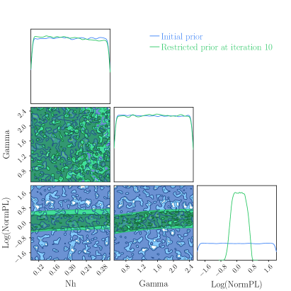
Figure 2: The initial and restricted prior, tuned to produce spectra that have between 10000 and 100000 counts for a tbabs x powerlaw model (at its tenth iteration). As can be seen, only a subset of parameters can deliver the right number of counts.

Let us assume a simple emission model consisting of an absorbed power law with three parameters: the column density ($N_{\rm H}$), the photon index (Gamma, $\Gamma$) and the normalization of the power law at 1 keV (NormPL). We used the tbabs model to take into account interstellar absorption, including the photoelectric cross-sections and the element abundances to the values provided by Verner et al. (1996) and Wilms et al. (2000), respectively. In XSPEC terminology, the model is tbabs x Powerlaw. For the simulations, we used NICER response files (for the observation identified in the NICER HEASARC archive as OBSID1050300108, see later). The simulated spectra are grouped in 5 consecutive channels so that each spectrum has $\sim 200$ bins covering the 0.3 and 10 keV range. We define the integration time of the simulated spectra, identical to all spectra and defined such that a reference model ($N_{\rm H}$=$0.2\times 10^{22}$ cm^-2, Gamma=$1.7$ and NormPL=1) corresponds to a spectrum with about 20000 counts. This spectrum provides the reference observation (referred as Spectrum₂₀₀₀₀counts). The initial range of prior is given in Table 1 for the model 1 set-up. We assume uniform priors in linear coordinates for $N_{\rm H}$ and for $\Gamma$ and in logarithmic coordinates for the power law normalisation. The generation of synthetic spectra is done within JAXspec, which offers parallelisation of a fakeit-like command in XSPEC (Dupourqué et al. in preparation). The generation of 10000 simulations takes about 10 seconds. We do not consider instrumental background, but note that if a proper analytical model exists for the background, the network could be trained to learn about the source and the background spectra simultaneously (with more free parameters than in the source alone case), at the expense of increasing the size of the training sample.

The first range of counts per spectrum to be probed is between 10000 and 100000, so that the above reference spectrum (Spectrum₂₀₀₀₀counts) is well covered. In Fig. 2, we show the initial and final round of the restricted prior, derived with the above condition. Given the integration time for the spectra, only a restricted set of model parameters can deliver the right number of counts per spectrum.

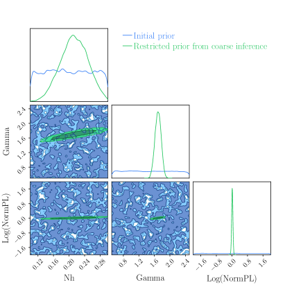
Figure 3: The initial and restricted prior computed from a coarse and quick inference of a reference spectrum of 20000 counts. Such a coarse inference can be seen as the first step of a multiple round inference.

The second method uses a coarse inference, and can be considered as the first step of a multiple round inference. A coarse inference is when the network is trained with a limited number of samples. The posterior conditioned at the reference observation is then used as the restricted prior. In Fig.  3, we present the result of a coarse inference of the above reference spectrum (Spectrum₂₀₀₀₀counts). 5000 spectra are generated from the initial prior as defined in Tab. 1 for the above model, fed to the neural network, and the posterior distributions are computed at the reference spectrum. The training for such a limited sample of simulation, for three parameters, takes about 1 minute. As can be seen, the prior range is further constrained to narrower intervals. Generating a sample of 10000 spectra with parameters from this restricted prior shows that the reference spectrum is actually close to the median of the sample of the simulated spectra (see Fig. 4). The robustness of SBI-NPE again local false minima trapping (see Sec. 6), guarantees good coverage of the observation from the restricted prior.

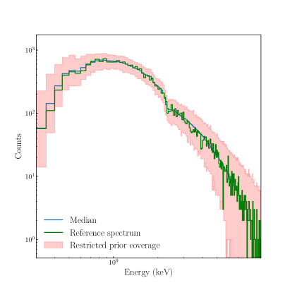
Figure 4: A prior predictive check showing that the coarse inference provides good coverage of the reference spectrum (Spectrum₂₀₀₀₀counts). The coverage of the restricted prior is indicated in red. The median of the spectra sampled from the restrictor (blue line) is to be compared with the reference spectrum (green line).

Starting from the restricted prior, one can then draw samples of $\vec{\theta}_{i}$ and generate spectra applying the Poisson count statistics in each spectral bin. The spectra are then binned the same way as the reference observation (grouped by 5 adjacent channels between 0.3 and 10 keV), and injected as such in the network (no zero mean scaling, no component reduction applied, see however Sec. 7). For each run, we generate both a training and an independent test sample.

4 Single round inference

We will consider two reference observation setups: one for which the number of counts per spectrum ranges between 10000-100000, and one in which it ranges from 1000-10000. For this, we apply the first method described above to get the restricted prior.

4.1 In the Gaussian regime

In the first case, we run the classifier with the condition that each of the simulated spectra assuming an absorbed power law model has between 10000–100000 counts, spread over $\sim 200$ bins. This covers the Gaussian regime.

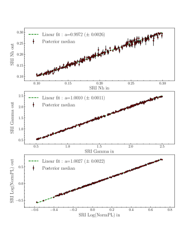
Figure 5: Inferred model parameters versus input model parameters for the case in which spectra have between 10000–100000 counts, spread over 200 bins. A single round inference is performed on an initial sample of 10000 simulated spectra. The median of the posterior distributions is computed from 20000 samples and the error on the median is computed from the 68% quantile of the distribution. The linear regression coefficient is computed for each parameter over the 500 test samples.

For three parameters, we generate a set of 10000 spectra. The network is trained in $\sim 2$ minutes. The inference is performed with the default parameters of SNPE_C as implemented in sbi, which is using 5 consecutive MADEs with 50 hidden states each for the density estimation. It then takes about the same time to draw 20000 posterior samples for 500 test spectra. The inferred model parameters versus the input parameters are shown in Fig.  5. As can be seen, there is an excellent match between the input and output parameters: the linear regression coefficient is very close to 1. For $N_{\rm H}$, a minimal bias is observed towards the edge of the sampled parameter space.

We generate the posterior distributions for the reference absorbed power law spectrum and compare it with the posterior distribution obtained from XSPEC  switching on Bayesian inference . The comparison is shown in Fig.  6. There is an excellent match between the best fit parameters, but also the posterior distribution, including their spread. In both cases, the C-stat of the best fit is within $1\sigma$ of the expected C-stat following Kaastra (2017). Note that running XSPEC to derive the posterior distribution takes about the same time as training the network.

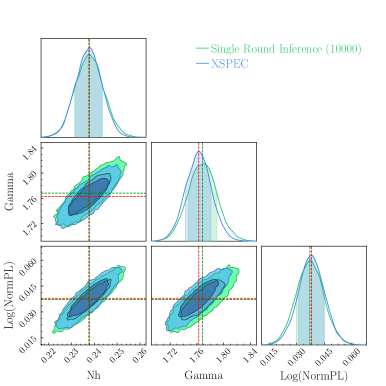
Figure 6: The posterior distribution estimated for the reference absorbed power law spectrum (Spectrum₂₀₀₀₀counts) as inferred from a single round inference with a network trained on 10000 samples (green). The posterior distribution inferred from a Bayesian fit with XSPEC is also shown in blue.

We now show the count spectrum corresponding to the reference spectrum of this run, together with the folded model and the associated residuals, in Fig. 7 for both SBI-NPE and XSPEC. As expected from Fig.  6, there is an excellent agreement between the fits with the two methods.

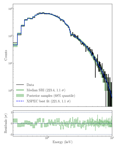
Figure 7: Top) The count spectrum corresponding to the reference absorbed power law spectrum (Spectrum₂₀₀₀₀counts), together with the folded best fit model from both SBI-NPE (green solid line) and XSPEC (blue dashed line). Bottom) The residuals of the best fit from SBI-NPE.

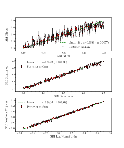
Figure 8: Inferred model parameters versus input model parameters for the case in which spectra have between 1000–10000 counts, spread over 200 bins. The neural network is trained with 20000 simulations and the posteriors for 500 test spectra are then computed. The medians of the posteriors are computed from 20000 samples and the error on the median is computed from the 68% quantile of the distribution. The linear regression coefficient is computed for each parameter over the 500 test samples.

4.2 In the Poisson regime

The above results can be considered as encouraging, but to test the robustness of the technique, we must probe the low count Poisson regime. We repeat the run above but this time generating spectra from a restricted prior generating 200 bin spectra with a number of counts ranging between 1000–10000 for the absorbed power law model. The integration time of the spectra is scaled down from the Gaussian case, so that the reference model ($N_{\rm H}$=$0.2\times 10^{22}$ cm^-2, Gamma=$1.7$ and NormPL=1) now corresponds to a spectrum of $\sim 2000$ counts (referred as Spectrum₂₀₀₀counts). To account for the lower statistics, we train the network with a sample of 20000 spectra, instead of 10000 for the case above. The training time still takes about 2 minutes. We generate the posterior for a test set of 500 spectra. Similar to Fig.  5, we show the input and inferred model parameters for the test sample in Fig. 8. As in the previous case, although with larger error bars, accounting for the lower statistics of the spectra, there is an excellent match between the two quantities, the linear regression coefficient remains close to 1, with some evidence for the small bias on $N_{\rm H}$ at both ends of the parameter range increased.

We generate the Posterior distribution for the reference spectrum (Spectrum₂₀₀₀counts), which we also fit with BXA (assuming the same priors as listed in Tab. 1 for the model 1 set-up). The posterior distributions are compared in Fig. 9, showing again an excellent agreement. Not only the best fit parameters are consistent with one another, but as important, the widths of the posterior distribution are also comparable. This demonstrates that SBI-NPE generates healthy posteriors. Note that the time to run BXA (without parallelization) on such a spectrum is comparable with the training time of the network.

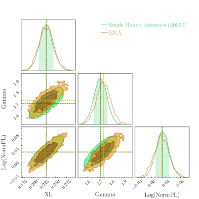
Figure 9: The posterior distributions for a reference spectrum of 2000 counts as derived from SBI-NPE with a single round inference of a network trained with 20000 samples (green) and by BXA in orange.

5 Multiple round inference

In the previous cases, the posterior is inferred using single-round inference. We are now considering multi-round inference, tuned for a specific observation; the reference spectrum of 2000 counts, spread over 200 bins (Spectrum₂₀₀₀counts). For the first iteration, from the restricted prior, we generate 1000 simulations, and train the network to estimate the posterior distribution. In each new round of inference, samples from the obtained posterior distribution conditioned at the observation (instead of from the prior) are used to simulate a new training set used for training the network again. This process can be repeated an arbitrary number of times. Here we stop after three iterations. In Fig. 10, we show that multi-round inference returns best fit parameters and posterior distributions consistent with single-round inference (from a larger training sample) and XSPEC. We thus confirm that multi-round inference can be more efficient than single round inference in the number of simulations and is faster in inference time. Its drawback is however that the inference is no longer amortized (i.e. it will only apply for a specific observation).

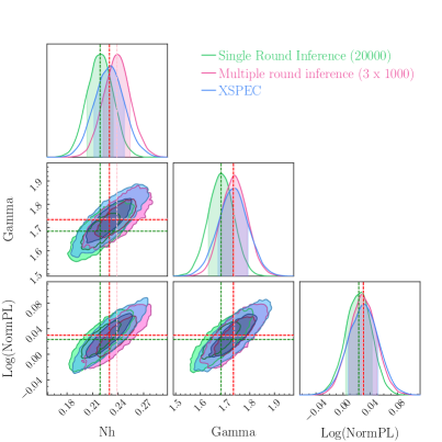
Figure 10: The posterior distributions for a reference spectrum of 2000 counts as derived from SBI-NPE with a single round inference of a network trained with 20000 samples (green), multiple round inference with three iterations, in which the network in trained with a sample of 1000 simulations (pink) and by XSPEC (blue).

6 Sensitivity to local minima

Fit statistic minimisation algorithms may get stuck into local false minima. There are different workarounds, such as computing the errors on the model parameters to explore a wider parameter space, shaking the fits with different sets of initial parameters, using Bayesian inference, all at the expense of increasing the processing times. We are now going to consider a 5 parameter model combining two overlapping components, a power law and a blackbody. In the XSPEC terminology, the model would be tbabs x (powerlaw + blackbody) (see Tab. 1 for the model 2 simulation set-up for the priors). We build a restricted prior so that such a model produces at least 10000 counts per spectrum, as decent statistics is required to constrain a 5 model parameters. We train a network with 100000 simulated spectra. We then generate the posterior of 500 spectra that we fit with XSPEC, with three sets of initial parameters: the model parameters, a set of model parameters generated from the restricted prior, a set of model parameters from the initial prior (that do not meet necessarily our requirement on counts). We switch off Bayesian inference in the XSPEC fits, and return for each of the fits, the best fit C-stat statistics. In Fig. 11, we compare the C-stat of SBI-NPE as derived from a single round inference with the XSPEC fitting. This figure shows that SBI-NPE does not produce outliers, while the minimisation does, at the level of a few percent. The latter is a known fact. The use of a restricted prior helps in reducing the trapping in local false minima, compared to considering the wider original prior because the XSPEC fits starts closer to the best fit parameters. The most favorable, and unrealistic, situation for XSPEC is when the fit starts from the model parameters. In some cases, SBI-NPE produces minimum C-stat that are slightly larger than those derived from XSPEC, indicating that the best fit solution was not reached. This may simply call for enlarging the training sample of the network for such a 5 parameter model, or considering multiple-round inference.

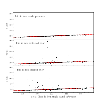
Figure 11: Comparison between XSPEC spectral fitting and SBI-NPE. The initial parameters of the XSPEC fits are the input model parameter (top panel), a set of parameters generated from the restricted prior (middle panel), and a set of parameters generated from the initial prior (bottom panell). The y-scale is the same for the three panels. Outliers away from the red line are due to XSPEC getting trapped in a local false minimum.

7 Dimension reduction with the Principal Component Analysis

Parker et al. (2022) introduced the use of principal component analysis (PCA) to reduce the dimension of the data to feed the neural network, and showed that it increased the accuracy of the parameter estimation, without any penalty on computational time, yet enabling simpler network architecture to be used. The PCA performs a linear dimensionality reduction using singular value decomposition of the data to project it to a lower dimensional space. Unlike Parker et al. (2022), we have here access to the posteriors and it is worth investigating whether such a PCA decomposition affects the uncertainty on the parameters estimates. Considering the run presented in Sec. 4 for the case of single round inference in the Poisson regime, we decompose the 20000 spectra with the PCA, as to keep 90% of their variance (before that we scale the spectra to have a mean of zero and standard deviation of 1). This allows to reduce the dimension of the data from $20000\times 200$ to $20000\times 60$, i.e. a factor of 3 reduction, leading to a gain in inference time by a factor of 2. We show in Fig. 12 the input and output parameters from a single round inference trained on dimension reduced data. As can be seen, there is still an excellent agreement between the two with the linear regression coefficient close to 1, although the bias on $N_{\rm H}$ at the edge of the prior interval seems to be more pronounced (the slopes for all parameters are less than 1, indicating that a small bias may have been introduced through the PCA decomposition).

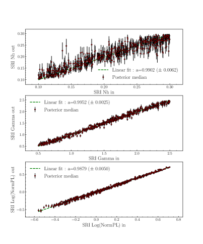
Figure 12: Inferred model parameters versus input model parameters for the case in which spectra have between 1000–10000 counts, spread over 200 bins. The best fit parameters are derived from a single round inference of a network trained by 20000 samples, reduced by the PCA, so that only 90% of the variance in the samples is kept.

We show the posteriors of the fit of the reference spectrum of 2000 counts, in comparison with XSPEC in Fig.  13 to show that the posteriors are not broadened by the dimension reduction.

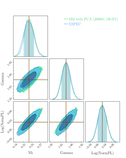
Figure 13: The posterior distributions for a reference spectrum of 2000 counts as derived from SBI-NPE with a single round inference of a network trained with 20000 samples (green) decomposed by the PCA (green, dimension reduced by a factor of 3) and XSPEC (blue).

8 Application to real data

Having shown the power of the technique on mock simulated data, it now remains to demonstrate its applicability to real data, recorded by an instrument observing a celestial source of X-rays (and not data generated by the same simulator used to train the network). This is a crucial step in machine learning applications.

We have considered NICER response files for the above simulations because we are now going to apply the technique to real NICER data recorded from 4U1820-303 (Gendreau et al., 2012; Keek et al., 2018). For the scope of the paper, we are going to consider two cases: a spectrum for the persistent X-ray emission (number of counts $\sim 200000$) and spectra recorded over a type I X-ray burst, when the X-ray emission shows extreme time and spectral variability.

8.1 NICER data analysis

We have retrieved the archival data of 4U1820-303 from HEASARC for the observation identifier (1050300108), and processed them with standard filtering criteria with the nicerl2 script provided as part of the HEASOFTV6.31.1 software suite, as recommended from the NICER data analysis web page (NICER software version : NICER_2022-12-16_V010a). Similarly, the latest calibration files of the instrument are used throughout this paper (reference from the CALDB database is xti20221001). A light curve was produced between 0.3 and 7 keV band, with a time resolution of 120 ms, so that the type I X-ray burst could be located precisely.

8.2 Spectrum of the persistent emission

Once the burst time was located, we first extract a spectrum of the persistent emission for 200 seconds, ending 10 seconds before the burst. The spectrum is then modelled by a 5-component model, as the sum of an absorbed sum of a blackbody and a power law. In XSPEC terminology, the model is tbabs x (blackbody+powerlaw). The initial range of prior is given in Tab. 1 for the model 2 set-up. For both SBI-NPE and XSPEC spectral fitting, for a change, we consider uniform priors in linear coordinates for all the parameters. Similarly, for this observation, we build a restricted prior with the condition that at each of the 10 rounds, the classifier keeps 25% of the model parameters associated with the lowest C-stat. From this restricted prior, we generate a rather conservative set of 100000 spectra for a single round inference, and a set of 5000 spectra for a multiple-round inference considering only three iterations. It takes about 40 minutes to train the network with 100000 spectra with 5 parameters, and 12 minutes for the 3 iteration multiple-round inference. The posterior distribution from single and multiple round inference, and the XSPEC fitting are shown in Fig.  14. As can be seen, there is a perfect match between XSPEC and SBI-NPE, demonstrating that the method is also applicable to real data. We have verified that changing the assumptions for the priors, e.g. uniform in logarithmic scale for the normalisations of both the blackbody and the power law, yielded fully consistent results, in terms of best fit parameters, C-stat and posterior distributions. The same applies when using BXA instead of XSPEC. This is the first demonstration to date that SBI-NPE performs equally well as state-of-the-art X-ray fitting techniques.

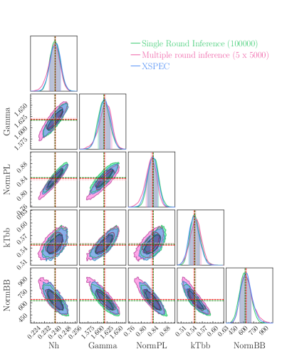
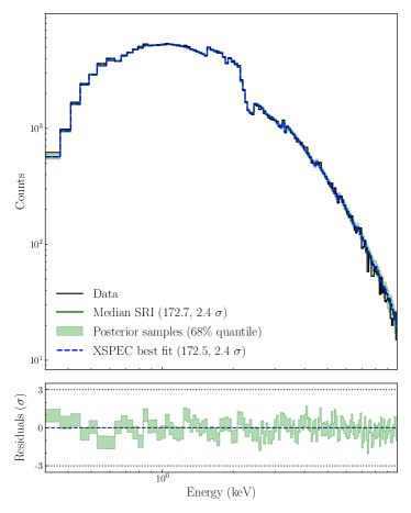
Figure 14: Left) Posterior distribution comparison between XSPEC spectral fitting and SBI-NPE, as applied to the persistent emission spectrum of 4U1820-303 (pre-burst). The spectrum is modelled as tbabs x (blackbody+powerlaw). There is a perfect match between the three methods, not only on the best fit parameters but also on the width of the posterior distributions. Right) The count spectrum of the persistent emission, together with the folded model derived from both SBI-NPE and XSPEC. The C-stat of the best fit is indicated together with its deviation against the expected value.

8.3 The burst emission

The first burst observed with NICER was reported by (Keek et al., 2018; Strohmayer et al., 2019; Yu et al., 2023). The burst emission is fitted with a blackbody model and a component accounting for some underlying emission, which in our case is assumed to be a simple power law. The blackbody temperature and its normalisation vary strongly along the burst itself, in particular in this burst, which showed the so-called photospheric expansion, meaning that the temperature of the blackbody drops while its normalisation increases, to raise again towards the end of the burst. To follow spectral evolution along the burst, we extract fixed duration spectra (0.25 seconds), still grouped in 5 adjacent channels, so that all the spectra have the same number of bins (200). The number of counts per spectrum ranges from 400 to 5000, hence offering the capability of exploring the technique with real data in the Poisson regime. In this range of statistics, we cannot constrain a 5-parameter model. Hence, we fix the column density and the power law index to $N_{\rm H}$=$0.2\times 10^{22}$ cm^-2 and $\Gamma=1.7$ respectively. The initial range of prior is given in Table 1 for the model 3 set-up.

As we want to use the power of amortized inference, we use two methods to define our training sample. First, we apply the classifier with the condition to keep the model parameters associated with spectra with a number of counts ranging between 100–10000, hence covering plainly the range of counts of the observed spectra. From the restricted, we consider arbitrarily 5000 simulated spectra per observed spectrum so that the network is trained with $23\times 5000=115000$ samples. Second, we perform a coarse inference over the full prior range, and for each of the 23 spectra, we set the restricted prior as the posterior conditioned at the corresponding spectrum. The training sample is limited to 10000 spectra for the quick and coarse inference of the 23 spectra. For each of the 23 restricted prior, we then generate 2500 simulated spectra so that their ensemble will be used to train the network, i.e. with $23\times 2500=57500$ samples. The predictive check of this prior is shown in Fig. 15, which indicates that such a build up prior covers all the observed spectra. The training then takes about $\sim 15$ minutes. The generation of the posterior samples takes $\sim 20$ seconds. We then fit the data with Bayesian inference with XSPEC. We then derive the errors on the fitted parameters using MCMC. As can be seen, SBI-NPE with amortized inference for the two different restricted priors can follow the spectral evolution along the burst, with an accuracy comparable to XSPEC, even when the number of counts in the spectra goes down to a few hundred, deep into the Poisson regime. The results of our fits are fully consistent with those reported by (Keek et al., 2018; Strohmayer et al., 2019; Yu et al., 2023). This provides further demonstration that SBI-NPE is applicable to real data, and that the power of amortization can still be used for multiple spectra showing wide variability.

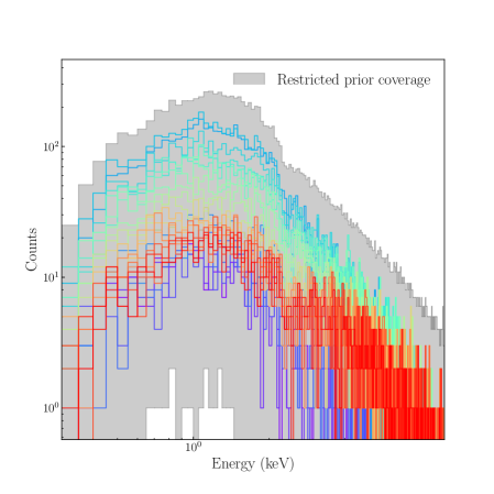
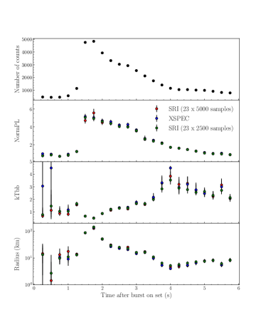
Figure 15: Left) 23 burst spectra covered by the restricted prior, indicated by the region in grey. Right) Recovered spectral parameters with SBI-NPE and XSPEC. The agreement between the different methods is remarkable. The figure shows the number of counts per spectrum (top), the normalisation of the power law, the temperature of the backbody in keV, and at the bottom the blackbody normalisation translated to a radius (in km) assuming a distance to the source of 8 kpc. Single Round Inference is performed with a training sample of $23\times 5000$ spectra, derived from a restrictor, constraining the number of counts in the spectra to be between 100 and 10000 counts (red filled circles). Single Round Inference is also performed with a training sample of $23\times 2500$ spectra, generated from a restrictor build from a quick inference (green filled circles). XSPEC best fit results are shown with blue filled circles.

9 Discussion

We have demonstrated the first working principles of SBI-NPE for X-ray spectral fitting for both simulated and real data. We have shown that not only it can recover the same best fit parameters as traditional X-ray fitting techniques, but delivers also healthy posteriors, comparable to those derived from Bayesian inference with XSPEC and BXA. The method works equally well in the Gaussian and Poisson regimes, with uncertainties reflecting the statistical quality of the data. The existence of a known likelihood helps to demonstrate that the method is well calibrated. We have still performed recommended checks, such as Simulation-Based Calibrations (SBC) (Talts et al., 2018): a procedure for validating inferences from Bayesian algorithms capable of generating posterior samples. SBC provides a (qualitative) view and a quantitive measure to check, whether the uncertainties of the posterior are well-balanced, i.e., neither over-confident nor under-confident. SBI-NPE as implemented here passed the SBC checks, as expected from the comparison of the posterior distributions with XSPEC and BXA.

We have shown SBI-NPE to be less sensitive to local false minima than classical minimisation techniques as implemented in XSPEC, consistent with the findings of Parker et al. (2022). We have shown that, although raw spectra can train the network, SBI-NPE can be coupled with Principal Component Analysis for reducing the dimensions of the data to train the network, offering potential speed improvements for the inference (Parker et al., 2022). For the simple models considered here, no broadening of the posterior distribution is observed. This kind of approach can be extended to various dimension reduction methods, since SBI-SNPE is not bound to any likelihood computation.

Multiple-round inference combined with a restricted prior is perfectly suited when dealing with a few observations. The power of amortization can also be used, even when the observations show large spectral variability, as demonstrated above. The consideration of a restricted prior, either on the interval of counts covered by the observation data sets or from a coarse fitting of the ensemble of observations with a small neural network used upfront, enables to define an efficient training sample, to cover the targeted observations. Note however that the use of a restricted prior can always be compensated by a larger sample size on an extended prior, with the penalty on the training time. The use of a classifier to restrict the range of priors, being easy to implement and running fast, can be coupled with standard X-ray fitting tools to increase their speed and decrease the risk to get trapped into local false minima.

Within the demonstration of the working principles of the technique, we have found that the training time of the neural network is shorter and/or comparable to state of the art fitting tools. The SBI framework used here is fully parallel, meaning that moving from a laptop (6 cores) to a cluster (e.g. 40 cores) will decrease the inference time proportionally, bringing it to the minute duration for the cases considered here. On the other hand, once the network has been trained, generating the posterior distribution is instantaneous compared to traditional fitting. This means that SBI-NPE holds great potential for integration in pipelines of data processing for massive data sets. The range of applications of the method has yet to be explored, but the ability to process a large sample of observations with the same network offers the opportunity to use it to track instrument dis-functioning, calibration errors, etc. This will be investigated for the X-IFU instrument on Athena (Barret et al., 2023).

We are aware that we have demonstrated the working principles of SBI-NPE, considering simple models, spectra with a relatively small number of bins. The applicability of the technique to more sophistical models, higher resolution spectra, such as those that will be provided by X-IFU, will have to be demonstrated, although the alternative tools, such as XSPEC and BXA, may have issues on their own in terms of processing time. Through this demonstration, we have already identified some aspects of the technique to keep investigating. For instance, an amortized network is applicable to an ensemble of spectra that must have the same binning/grouping, the same exposure time… The later could be relaxed if one is not interested in the normalisation of the model components (flux), but just the variations of the other parameters (e.g. Gamma of a power law). There is no easy work around for this. Obviously, there are many cases when the above conditions will be met, e.g. when dealing with an observation for which we are interested in probing spectral variability on some timescales, as we have shown above in the case of a type I X-ray burst. Once the network has been trained, the generation of posteriors being instantaneous, SBI-NPE makes it possible to track model parameter variations on timescales much shorter than what is possible today with existing tools.

The quality of the training depends on the size of the training sample. There is no rule yet to define the minimum sample size. Similarly, for multiple-round inference, the number of iterations is a free parameter, that may need some fine-tuning to ensure that convergence to the best fit solution has been reached. The existence of alternative robust tools such as XSPEC and BXA will help to define guidelines. For complex multi-component spectra, the size of the training sample will have to be increased. The use of a restricted prior will always help, but considering dimension reduction, e.g. decomposition in principal components, or the use of an embedding network to extract the relevant summary features of the data, may become mandatory. Any loss of information will have an impact on the inference itself. Another limitation may come from the time to generate the simulations to train the network. Here we have used simple models and a fully parallel version of the XSPEC fakeit developed within JAXspec (Dupourqué et al. in preparation). This was not a limiting factor for this work, so we plan to release JAXspec to the community to further support the development and use of SBI-NPE for X-ray spectral fitting.

The python scripts from which the results have been derived are based on the sbi package (Tejero-Cantero et al., 2020). They are straightforward to use and will be made available through GitHub for broadening the use of SBI-NPE by the community.

10 Conclusions and way forward

We have demonstrated for the first time the working principles of fitting X-ray spectra with simulation-based inference with neural posterior estimation, down to the Poisson regime. We have applied the technique to real data, and demonstrated that SBI-NPE converges to the same best fit parameters and provides fitting errors comparable to Bayesian inference. We may therefore be at the eve of a new era for X-ray spectral fitting, but more work is needed to demonstrate the wider applicability of the technique to more sophisticated models and higher resolution spectra, and in particular to those provided by the new generation of instruments, such as the X-IFU spectrometer to fly on-board Athena. Yet, along this work, we have not identified any show-stoppers for this not to be achievable. Certainly, the pace at which machine learning applications develop across so many fields will also help in solving any issues that we may have to face, strengthening the case for developing further the potential of Simulation-Based Inference with Neural Posterior Estimation for X-ray spectral fitting.

11 Acknowledgements

DB would like to thank all the colleagues who shared their unfortunate experience of getting stuck, without knowing, into local false minima, when doing X-ray spectral fitting. The fear of ignoring that the true global minimum is just nearby is what motivated this work in the first place with the hope of preventing sleepless nights in the future. DB is also grateful to all his X-IFU colleagues, in particular from CNES, for developing such a beautiful instrument that will require new tools, such as the one introduced here, for analyzing the high quality data that it will generate. DB/SD thank Alexei Molin and Erwan Quintin for their support and encouragements along this work.

12 Python software packages used

In addition to the sbi package (Tejero-Cantero et al., 2020), this work made use of many awesome Python packages: ChainConsumer (Hinton, 2016), matplotlib (Hunter, 2007), numpy (Harris et al., 2020), pandas (McKinney, 2010), pytorch (Paszke et al., 2017), scikit-learn (Pedregosa et al., 2011), scypi (Virtanen et al., 2020), tensorflow (Abadi et al., 2015).

References

- Abadi et al. (2015) Abadi, M., Agarwal, A., Barham, P., et al. 2015, TensorFlow: Large-Scale Machine Learning on Heterogeneous Systems, software available from tensorflow.org
- Arnaud (1996) Arnaud, K. A. 1996, in Astronomical Society of the Pacific Conference Series, Vol. 101, Astronomical Data Analysis Software and Systems V, ed. G. H. Jacoby & J. Barnes, 17
- Barret et al. (2023) Barret, D., Albouys, V., Herder, J.-W. d., et al. 2023, Experimental Astronomy, 55, 373
- Bevington & Robinson (2003) Bevington, P. & Robinson, D. 2003, Data Reduction and Error Analysis for the Physical Sciences (McGraw-Hill Education)
- Buchner (2021) Buchner, J. 2021, Journal of Open Source Software, 6, 3001
- Buchner & Boorman (2023) Buchner, J. & Boorman, P. 2023, arXiv e-prints, arXiv:2309.05705
- Buchner et al. (2014) Buchner, J., Georgakakis, A., Nandra, K., et al. 2014, A&A, 564, A125
- Cash (1979) Cash, W. 1979, ApJ, 228, 939
- Cranmer et al. (2020) Cranmer, K., Brehmer, J., & Louppe, G. 2020, Proceedings of the National Academy of Science, 117, 30055
- Crisostomi et al. (2023) Crisostomi, M., Dey, K., Barausse, E., & Trotta, R. 2023, Phys. Rev. D, 108, 044029
- Deistler et al. (2022) Deistler, M., Goncalves, P. J., & Macke, J. H. 2022, arXiv e-prints, arXiv:2210.04815
- Deistler et al. (2022) Deistler, M., Macke, J. H., & Gonçalves, P. J. 2022, Proceedings of the National Academy of Sciences, 119, e2207632119
- Gendreau et al. (2012) Gendreau, K. C., Arzoumanian, Z., & Okajima, T. 2012, in Society of Photo-Optical Instrumentation Engineers (SPIE) Conference Series, Vol. 8443, Space Telescopes and Instrumentation 2012: Ultraviolet to Gamma Ray, ed. T. Takahashi, S. S. Murray, & J.-W. A. den Herder, 844313
- Germain et al. (2015) Germain, M., Gregor, K., Murray, I., & Larochelle, H. 2015, in Proceedings of the 32nd International Conference on Machine Learning (PMLR), 881–889, iSSN: 1938-7228
- Goodman & Weare (2010) Goodman, J. & Weare, J. 2010, Communications in Applied Mathematics and Computational Science, 5, 65
- Graber et al. (2023) Graber, V., Ronchi, M., Pardo-Araujo, C., & Rea, N. 2023, arXiv e-prints, arXiv:2312.14848
- Greenberg et al. (2019) Greenberg, D. S., Nonnenmacher, M., & Macke, J. H. 2019, arXiv e-prints, arXiv:1905.07488
- Greenberg et al. (2019) Greenberg, D. S., Nonnenmacher, M., & Macke, J. H. 2019, Automatic Posterior Transformation for Likelihood-Free Inference, arXiv:1905.07488 [cs, stat]
- Harris et al. (2020) Harris, C. R., Millman, K. J., van der Walt, S. J., et al. 2020, Nature, 585, 357
- He et al. (2015) He, K., Zhang, X., Ren, S., & Sun, J. 2015, Deep Residual Learning for Image Recognition
- Hinton (2016) Hinton, S. R. 2016, The Journal of Open Source Software, 1, 00045
- Hunter (2007) Hunter, J. D. 2007, Computing in science & engineering, 9, 90
- Huppenkothen & Bachetti (2022) Huppenkothen, D. & Bachetti, M. 2022, MNRAS, 511, 5689
- Ichinohe et al. (2018) Ichinohe, Y., Yamada, S., Miyazaki, N., & Saito, S. 2018, MNRAS, 475, 4739
- Kaastra (2017) Kaastra, J. S. 2017, A&A, 605, A51
- Keek et al. (2018) Keek, L., Arzoumanian, Z., Chakrabarty, D., et al. 2018, ApJ, 856, L37
- Khullar et al. (2022) Khullar, G., Nord, B., Ćiprijanović, A., Poh, J., & Xu, F. 2022, Machine Learning: Science and Technology, 3, 04LT04
- Kobyzev et al. (2021) Kobyzev, I., Prince, S. J. D., & Brubaker, M. A. 2021, IEEE Transactions on Pattern Analysis and Machine Intelligence, 43, 3964, arXiv:1908.09257 [cs, stat]
- Lueckmann et al. (2017) Lueckmann, J.-M., Goncalves, P. J., Bassetto, G., et al. 2017, arXiv e-prints, arXiv:1711.01861
- McKinney (2010) McKinney, W. 2010, in Proceedings of the 9th Python in Science Conference, ed. S. van der Walt & J. Millman, 51 – 56
- Papamakarios & Murray (2016) Papamakarios, G. & Murray, I. 2016, arXiv e-prints, arXiv:1605.06376
- Papamakarios et al. (2021) Papamakarios, G., Nalisnick, E., Rezende, D. J., Mohamed, S., & Lakshminarayanan, B. 2021, Normalizing Flows for Probabilistic Modeling and Inference, arXiv:1912.02762 [cs, stat]
- Papamakarios et al. (2017) Papamakarios, G., Pavlakou, T., & Murray, I. 2017, in Advances in Neural Information Processing Systems, Vol. 30 (Curran Associates, Inc.)
- Parker et al. (2022) Parker, M. L., Lieu, M., & Matzeu, G. A. 2022, MNRAS, 514, 4061
- Paszke et al. (2017) Paszke, A., Gross, S., Chintala, S., et al. 2017, in NIPS Autodiff Workshop
- Pedregosa et al. (2011) Pedregosa, F., Varoquaux, G., Gramfort, A., et al. 2011, Journal of Machine Learning Research, 12, 2825
- Strohmayer et al. (2019) Strohmayer, T. E., Altamirano, D., Arzoumanian, Z., et al. 2019, ApJ, 878, L27
- Talts et al. (2018) Talts, S., Betancourt, M., Simpson, D., Vehtari, A., & Gelman, A. 2018, arXiv e-prints, arXiv:1804.06788
- Tejero-Cantero et al. (2020) Tejero-Cantero, A., Boelts, J., Deistler, M., et al. 2020, The Journal of Open Source Software, 5, 2505
- Vasist et al. (2023) Vasist, M., Rozet, F., Absil, O., et al. 2023, A&A, 672, A147
- Verner et al. (1996) Verner, D. A., Ferland, G. J., Korista, K. T., & Yakovlev, D. G. 1996, ApJ, 465, 487
- Virtanen et al. (2020) Virtanen, P., Gommers, R., Oliphant, T. E., et al. 2020, Nature Methods
- Wilms et al. (2000) Wilms, J., Allen, A., & McCray, R. 2000, ApJ, 542, 914
- Yu et al. (2023) Yu, W., Li, Z., Lu, Y., et al. 2023, arXiv e-prints, arXiv:2312.16420