Propagating terrace in a two-tubes model of gravitational fingering

Abstract

We study a semi-discrete model for the two-dimensional incompressible porous medium (IPM) equation describing gravitational fingering phenomenon. The model consists of a system of advection-reaction-diffusion equations on concentration, velocity and pressure, describing motion of miscible liquids under the Darcy’s law in two vertical tubes (real lines) and interflow between them. Our analysis reveals the structure of gravitational fingers in this simple setting – the mixing zone consists of space-time regions of constant intermediate concentrations and the profile of propagation is characterized by two consecutive traveling waves which we call a terrace. We prove the existence of such a propagating terrace for the parameters corresponding to small distances between the tubes. This solution shows the possible mechanism of slowing down the fingers’ growth due to convection in the transversal direction. The main tool in the proof is a reduction to pressure-free transverse flow equilibrium (TFE) model using geometrical singular perturbation theory and the persistence of stable and unstable manifolds under small perturbations.

Keywords. propagating terrace, porous media, Darcy’s law, gravitational fingering, geometric singular perturbation theory, invariant manifolds.

1 Introduction

In this paper, we consider the semi-discrete model of the 2D viscous incompressible porous media (IPM) equation. The IPM equation describes evolution of concentration carried by the flow of incompressible fluid that is determined via Darcy’s law in the field of gravity:

$$\partial_{t}c+\mathrm{div}(uc) =\nu\Delta c,\quad$$ (1)

$$\mathrm{div}(u) =0,$$ (2)

$$u =-\nabla p-(0,c).$$ (3)

Here $c=c(t,x,y)$ is the transported concentration, $u=u(t,x,y)$ is the vector field describing the fluid motion, $p=p(t,x,y)$ is the pressure, and $\nu\geq 0$ is a dimensionless parameter equal to an inverse of the Peclet number. The spatial domain $(x,y)$ can be either the whole space $\mathbb{R}^{2}$ or cylinder $[0,1]\times\mathbb{R}$ with periodic boundary conditions. In what follows, we will consider a discretization in $x$.

There have been many recent papers analyzing the well-posedness questions for the inviscid IPM equation ($\nu=0$) [10, 11], lack of uniqueness of weak solutions [12, 43] and questions of long time dynamics [10, 15, 8]. The question of global regularity vs finite-time blow up is open for the IPM equation, see e.g. [23].

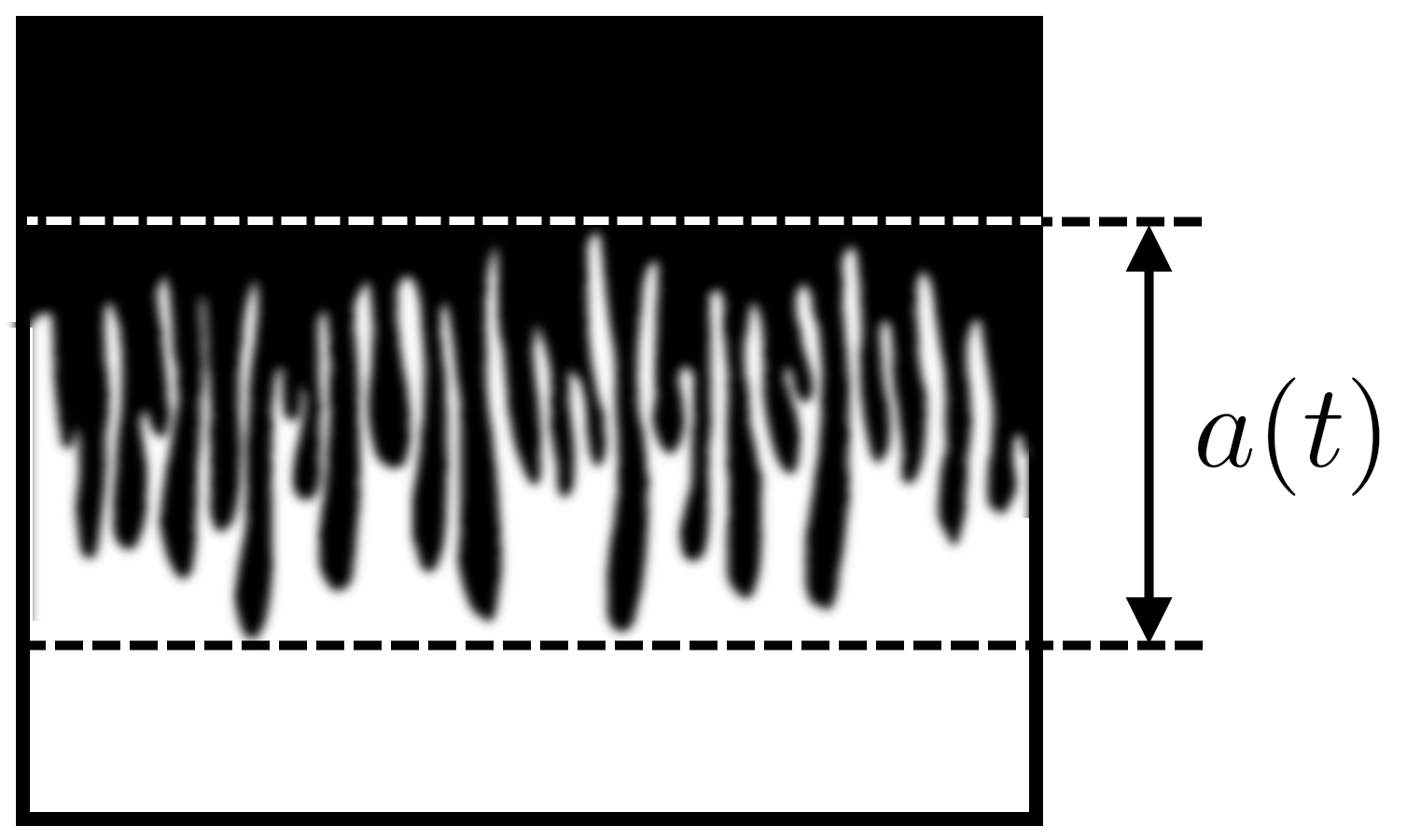
We are interested in studying the pattern formation for the initial conditions close to the unstable stratification:

$$c(0,x,y)=\begin{cases}+1,&y\geq 0,\\ -1,&y<0.\end{cases}$$ (4)

This corresponds to the heavier fluid on top and lighter on the bottom, and results into unstable displacement, as on Fig. 1, also known as gravitational fingering phenomenon. Fingering instability appears in subsurface [35], environmental [26, 32, 7], engineering [1], biological [28, 6], and petroleum engineering applications [2, 41, 42, 50]. In particular, the related problem of miscible viscous fingering appears in petroleum industry when a fluid of higher mobility displaces another of lower mobility (e.g., in the context of enhanced oil recovery (EOR) methods: polymer or gas flooding, important role plays speed of growth of the mixing zone [40, 25, 38, 18, 4, 44, 39]). In this case the analogue of Darcy’s law (3) reads as:

$$u =-K\cdot m(c)\nabla p.$$ (5)

Here $K$ is the porous media permeability tensor and $m(c)$ — the mobility function. Equations (1), (2), and (5) are called Peaceman model [34].

Figure 1: Schematic gravitation fingering instability, $a(t)$ — size of the mixing zone

For the inviscid IPM, this is the classical Saffman-Taylor instability. In [36], Saffman and Taylor discovered a one-parameter family of traveling wave solutions (which they called “fingers”). For the viscous IPM, the dynamics is distinguished by three regimes: (i) at early times, the flow is well described by linear stability theory; (ii) at intermediate times, the flow is dominated by nonlinear finger interactions which evolve into a mixing zone; and (iii) at late times.

Many laboratory and numerical experiments show the linear growth of the mixing zone for moderate time regimes (viscous fingering: e.g. [33, 5, 3], gravitational fingering: [27, 48]; see also surveys [22, 37]). A theoretical approach to estimate the width $a(t)$ of the mixing zone for the system (1)–(3) was done in [30]. In particular, the authors get $a(t)\leq 4t$ using energy estimates, and provide pointwise estimates

$$a(t)\leq 2t$$ (6)

for a reduced model that we call transverse flow equilibrium (TFE, see details in Section 2), for generalisations see [29, 49]. Quantification of the size of the mixing zone in laboratory and numerical experiments does not give exact answer: it shows that $a(t)\sim ct$ where the value of $c$ is a number in interval $c\in[1.786,2]$, see [27, 48, 37].

Our motivation is to understand the mechanism of finger formation and sharpen existing estimates for the size of the mixing zone. We show in a simplified setting that there are two (interconnected) mechanisms of possible slowing down of the fingers: (1) the convection in the transverse direction of the flow; (2) intermediate concentration, that is the typical concentration inside the finger is $c^{*}\in(-1,1)$. In particular, our results suggest that estimates (6) could be improved. While the difference between values $1.786$ and $2$ is not so large, it was shown in [3] that, for the case of viscous fingers, intermediate concentration could lead to a significant mixing zone slowdown.

In this paper, we introduce a new model for the gravitational fingering motivated by a finite-volume scheme with a simple upwind [14], that is widely used in multiphase flow simulations [16]. Our basic assumption is that the fluid displacement happens inside two vertical lines (“tubes”), and the transverse flow between the tubes is governed by the discrete Darcy’s law: the velocity is equal to the pressure difference divided by the distance between the tubes. This results in a system of nonlinear reaction-diffusion-convection equations that we call the two-tubes IPM equations.

More precisely, consider the two tubes denoted by 1 and 2. The model we study reads ($y\in\mathbb{R}$, after rescaling we can take $\nu=1$)

$$\partial_{t}c_{1}+\partial_{y}(u_{1}c_{1})-\partial_{yy}c_{1} =-f,$$

$$\partial_{t}c_{2}+\partial_{y}(u_{2}c_{2})-\partial_{yy}c_{2} =f.$$

Here $c_{1,2}=c_{1,2}(t,y)$ are the concentrations and $u_{1,2}=u_{1,2}(t,y)$ are the velocities in tube 1 and 2. Meanwhile the function $f$ is responsible for the flow between the tubes and is defined by

$$f=\begin{cases}w\cdot c_{1},&w\geq 0,\quad\text{(fluid flows from tube 1 to 2)},\\ w\cdot c_{2},&w\leq 0,\quad\text{(fluid flows from tube 2 to 1)}.\end{cases}$$

Figure 2:
Two tubes

Here $w=w(t,y)$ is the velocity of the fluid in the transversal direction to the tubes. The system of equations becomes closed if we supply it with expressions for the fluid velocities $u_{1,2}$ and $w$, analogous to equations (2)–(3), see Section 2 for the complete description. Let us point out that the transverse velocity $w$ is inversely proportional to the distance between the tubes $l$. The parameter $l$ plays a crucial role in our analysis.

Figure 3: Numerical evidence of propagating terrace consisting of two traveling waves

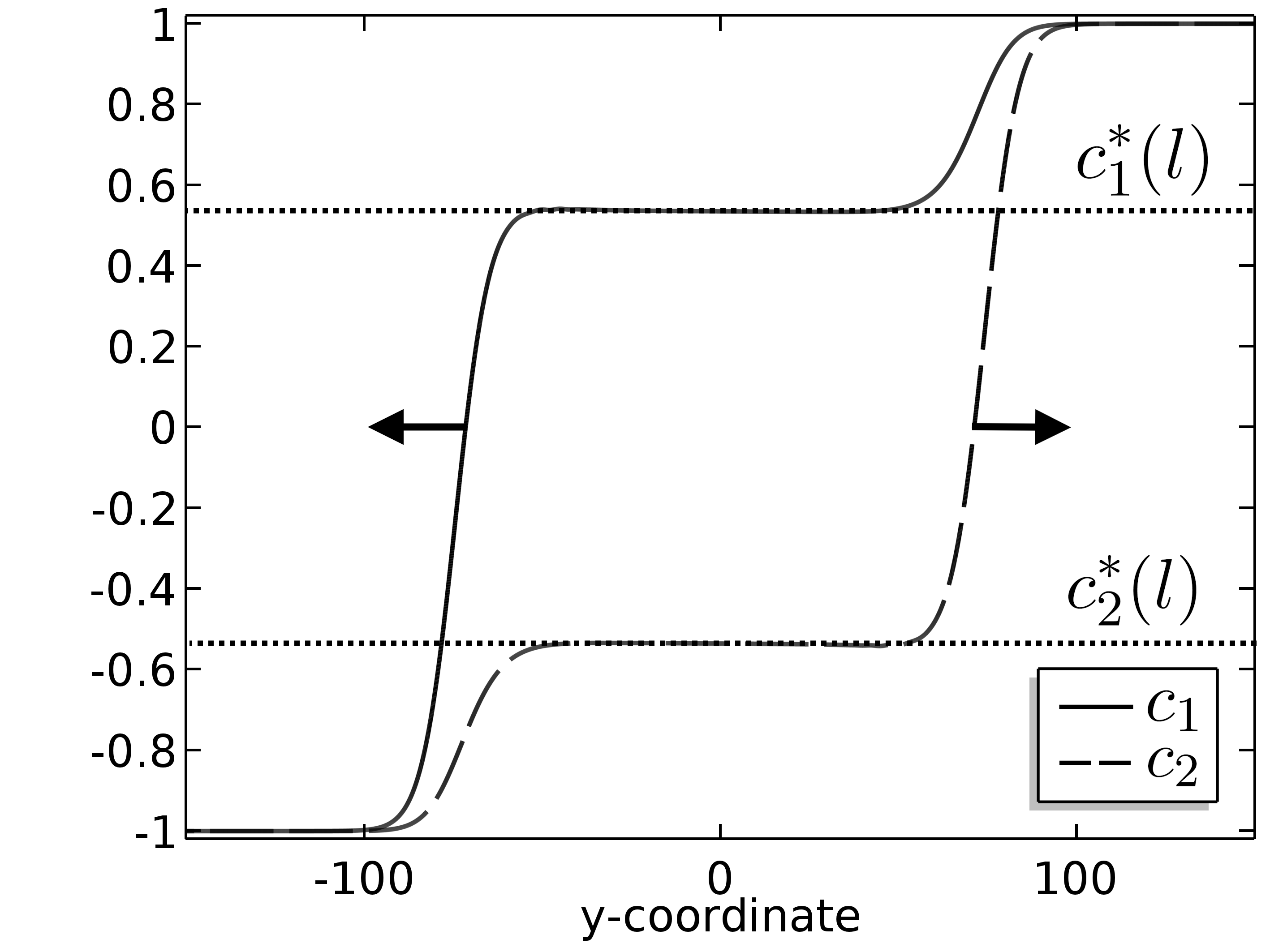
The main result (Theorem 1) claims that for sufficiently small values of $l>0$ there exist two intermediate concentrations $c_{1}^{*}(l)\in(-1,1)$, $c_{2}^{*}(l)\in(-1,1)$ and two traveling wave (TW) solutions that connect the states:

$$(-1,-1)\xrightarrow{TW}(c_{1}^{*}(l),c_{2}^{*}(l))\xrightarrow{TW}(1,1).$$

Moreover, the speeds of the traveling waves approach $-1/4$ and $1/4$ as $l\to 0$. The numerical modelling of the two-tubes IPM model, see Fig. 3, shows that such combination of two traveling waves (we will call it a propagating terrace) appears as a long-term limit for typical initial data with proper values at infinity.

The second main result (Theorem 2) establishes the existence and uniqueness of a propagating terrace for the two-tubes analogue of the TFE model. Surprisingly, in Theorem 2 we managed to find explicitly the trajectories of the traveling wave dynamical system. Note that each of the traveling waves connecting

$$(-1,-1)\xrightarrow{TW}(c_{1}^{*},c_{2}^{*})\quad\text{or}\quad(c_{1}^{*},c_{2}^{*})\xrightarrow{TW}(1,1)$$

exists for a one-parameter family of $(c_{1}^{*},c_{2}^{*})$, but the propagating terrace

$$(-1,-1)\xrightarrow{TW}(c_{1}^{*},c_{2}^{*})\xrightarrow{TW}(1,1)$$

is unique.

There is an important relation between the proofs of Theorem 1 and Theorem 2. Traveling wave dynamical system corresponding to the TFE model is a formal singular limit as $l\to 0$ of traveling wave dynamical system corresponding to the IPM model. Using geometric singular perturbation theory and invariant manifolds it is possible to extend properties of heteroclinic trajectories from the TFE system to the IPM system with sufficiently small $l>0$. See the end of Section 2 for details.

Propagating fronts in the layered media appear in different contexts: multilane traffic flow [21], combustion [31], and foam flow [45] in porous media in layers with different properties (permeabilities, porosities, thermal conductivities etc), voltage conduction along the nerve fibers [9].

The novel model we present here is natural and simple, illustrates the possible mechanism of the reducing the speed of fingers due to interflow between the tubes, while at the same time allowing for a rigorous mathematical treatment.

The paper is organised as follows: in Section 2 we formulate the two-tubes model (for IPM and TFE) and state the main results — Theorem 1 and Theorem 2 — the existence of solution in a form of a propagating terrace consisting of two traveling waves. Also we provide a sketch of the proofs. In Section 3 we give a proof of Theorem 2 for the two-tubes TFE model. In Section 4 we give a proof of Theorem 1 for the two-tubes IPM model. Section 5 is devoted to discussions and possible generalizations.

2 Problem statement and main result

Our aim is to consider the simple setting in which we can analyze the impact of the flow in transverse direction (with respect to gravity) on the speed of propagation of the mixing zone. The idea is to consider IPM equations (1)–(3) and discretize the space in $x$ direction.

In this paper, we focus on the simplest possible formulation — the case of two tubes. The $n$-tubes model, $n>2$, is discussed in [14]. Let $c_{1,2}(t,y)$ be the concentrations and $u_{1,2}(t,y)$ be the velocities in tube 1 and 2. Then the governing equations of the flow inside each tube are:

$$\partial_{t}c_{1}+\partial_{y}(u_{1}c_{1})-\partial_{yy}c_{1} =-f,$$ (7)

$$\partial_{t}c_{2}+\partial_{y}(u_{2}c_{2})-\partial_{yy}c_{2} =f.$$ (8)

The flow $f$ from tube 1 to tube 2 equals:

$$f=\begin{cases}w\cdot c_{1},&w\geq 0,\\ w\cdot c_{2},&w\leq 0.\end{cases}$$ (9)

Here $w=w(t,y)$ is the velocity of the fluid in the transversal direction to the tubes.

Let $p_{1,2}(t,y)$ be the pressures in tubes 1 and 2. The analogue of the Darcy’s law (3), is the following relation between the pressure and velocity:

(Darcy’s law in tube 1 and 2) $$u_{1} =-\partial_{y}p_{1}-c_{1}, u_{2} =-\partial_{y}p_{2}-c_{2},$$ (10)

(Darcy’s law between tubes) $$w =\frac{p_{1}-p_{2}}{l}.$$ (11)

Here $l>0$ is a parameter that corresponds to the distance between the tubes. The semi-discrete analogue of condition (2) writes as:

$$w+\partial_{y}u_{1}=0,\quad-w+\partial_{y}u_{2}=0.$$ (12)

We call the system (7)–(12) the two-tubes IPM equations.

Instead of considering the pressures $p_{1}$ and $p_{2}$ individually, the natural variable to consider is the pressure drop $q:=p_{2}-p_{1}$. Thus, the equations (10)–(12) can be simplified

$$\partial_{y}q =u_{1}-u_{2}+c_{1}-c_{2}, \partial_{y}u_{1} =q/l=-w.$$ (13)

Moreover, relations (12) imply $\partial_{y}(u_{1}+u_{2})=0$. As we assume later the conditions (15), we deduce

$$u_{1}+u_{2}\equiv 0.$$ (14)

Remark 1.

One can think of the model (7)–(12) as a limit of the finite-volume discretization of the model (1)–(3) with spatial grid $2\times N$ cells as $N\to\infty$, see [14] for details. Equation (9) corresponds to upwind scheme.

Remark 2.

To see an analogue of parameter $l$ in the two-dimensional IPM (1)-(3), we need to consider anisotropic permeability tensor in equation (3):

$$u=-\left(\begin{matrix}k_{x}&0\\ 0&k_{y}\end{matrix}\right)\nabla p-(0,c).$$

Notice that $l\to 0$ corresponds to $k_{y}/k_{x}\to 0$.

We are interested in finding solutions $(c_{1},c_{2},u_{1},u_{2},q)$ of (7)–(9), (13), (14) satisfying the following conditions at $\pm\infty$ (physical meaning — heavier fluid up, lighter fluid down; no flow inside the tubes and between them at $\pm\infty$):

$$c_{1,2}(-\infty)=-1,\qquad c_{1,2}(+\infty)=1,\qquad q(\pm\infty)=0,\qquad u_{1,2}(\pm\infty)=0.\qquad$$ (15)

Recall that a function $g(t,y):\mathbb{R}_{+}\times\mathbb{R}\to\mathbb{R}^{n}$, $n\in\mathbb{N}$, is a traveling wave with speed $v\in\mathbb{R}$ connecting states $g_{-}\in\mathbb{R}^{n}$ and $g_{+}\in\mathbb{R}^{n}$, if it has the form $g(t,y)=\tilde{g}(y-vt)$, where $\tilde{g}:\mathbb{R}\to\mathbb{R}^{n}$ is a continuous function, which satisfies $\tilde{g}(-\infty)=g_{-}$, $\tilde{g}(+\infty)=g_{+}$.

Numerically, we observe convergence of the solution of (7)–(9), (13), (14) to a combination of two traveling waves. Following [13], we introduce a notion of propagating terrace for our context.

Definition 1.

A propagating terrace connecting $\alpha\in\mathbb{R}^{5}$ to $\beta\in\mathbb{R}^{5}$ is a pair of finite sequences $(\sigma_{k})_{0\leq k\leq N}$ and $(g_{k})_{1\leq k\leq N}$ such that:

• Each $\sigma_{k}=(c_{1k},c_{2k},u_{1k},u_{2k},q_{k})$ is a stationary solution of (7)–(9), (13), (14) and $\sigma_{0}=\alpha$, $\sigma_{N}=\beta$.

• $g_{k}$ is a traveling wave solution of (7)–(9), (13), (14) connecting $\sigma_{k-1}$ to $\sigma_{k}$, $1\leq k\leq N$.

• The speed $v_{k}\in\mathbb{R}$ of each $g_{k}$ satisfies $v_{1}\leq v_{2}\leq\ldots\leq v_{N}$.

The following theorem is the first main result of the paper.

Theorem 1.

Consider the two-tubes IPM equations (7)–(9), (13), (14). Then there exists sufficiently small $l_{0}>0$ such that for all $l\in(0,l_{0})$ there exist a propagating terrace of two traveling waves with speeds $v_{1}^{*}(l)$, $v_{2}^{*}(l)$ connecting the states $\sigma_{0}=(-1,-1,0,0,0)$, $\sigma_{1}=(c_{1}^{*}(l),c_{2}^{*}(l),u_{1}^{*}(l),u_{2}^{*}(l),0)$, $\sigma_{2}=(1,1,0,0,0)$. Moreover, as $l\to 0$ we obtain:

$$\lim\limits_{l\to 0}c_{1}^{*}(l)=-\lim\limits_{l\to 0}c_{2}^{*}(l)=1/2, \lim\limits_{l\to 0}v_{2}^{*}(l)=-\lim\limits_{l\to 0}v_{1}^{*}(l)=1/4.$$

The proof of Theorem 1 is based on the fine analysis of the auxiliary system. Consider the so-called transverse flow equilibrium (TFE) model for velocities:

$$u_{1}=(c_{2}-c_{1})/2; u_{2}=-u_{1}.$$ (16)

This is a discrete analogue of the two-dimensional model originally introduced in [48], and analyzed in [30]. We call the system (7)–(9), (12), (16) the two-tubes TFE equations.

Remark 3.

In a similar way to Definition 1 the notion of the propagating terrace can be introduced for the two-tubes TFE equations. In this case $\sigma_{k}=(c_{1k},c_{2k}),\alpha,\beta\in\mathbb{R}^{2}$.

The second principal result of the paper is stated as follows.

Theorem 2.

Consider the two-tubes TFE equations (7)–(9), (12), (16). Then there exist exactly two propagating terraces of two traveling waves with speeds $v_{1}^{*}=-1/4$, $v_{2}^{*}=1/4$ connecting the states $\sigma_{0}=(-1,-1)$, $\sigma_{1}=(1/2,-1/2)$ $($or $\sigma_{1}=(-1/2,1/2))$, $\sigma_{2}=(1,1)$.

Theorem 2 can be interpreted in the following way: the width of the mixing zone for the two-tubes TFE equations is $a(t)\sim\frac{1}{2}t$, which means a slowdown compared to estimates (6). We believe that the interflow between the tubes and the presence of the intermediate concentration are responsible for such behavior.

See Remark 8 explaining an obstruction to prove uniqueness of the traveling wave solutions in Theorem 1 in contrast to Theorem 2.

The general scheme of the proof is common for Theorem 1 and Theorem 2 and states as follows (see Fig. 4 for the illustration):

1. For each $v_{1}$ in some interval $[d_{1}^{*},d_{2}^{*}]\subset\mathbb{R}$ we find the state $\sigma_{1}^{*}(v_{1})$, such that there exists a traveling wave solution with speed $v_{1}$ connecting $\sigma_{0}$ with $\sigma_{1}^{*}(v_{1})$. The set $\mathcal{H}_{-1}=\{\sigma_{1}^{*}(v_{1}):v_{1}\in[d_{1}^{*},d_{2}^{*}]\}$ forms a curve.

2. For each $v_{2}$ in some interval $[d_{1}^{**},d_{2}^{**}]\subset\mathbb{R}$ we find the state $\sigma_{1}^{**}(v_{2})$, such that there exists a traveling wave solution with speed $v_{2}$ connecting $\sigma_{1}^{**}(v_{2})$ with $\sigma_{2}$. The set $\mathcal{H}_{1}=\{\sigma_{1}^{**}(v_{2}):v_{2}\in[d_{1}^{**},d_{2}^{**}]\}$ also forms a curve.

3. Finally, we show that the two curves $\mathcal{H}_{1}$ and $\mathcal{H}_{-1}$ intersect, and the intersection point gives the values of the intermediate state $\sigma_{1}$ and the speeds $v_{1}$, $v_{2}$.

Remark 4.

On the first sight for the IPM case it may seem surprising to expect the two curves $\mathcal{H}_{1},\mathcal{H}_{-1}\subset\mathbb{R}^{5}$ to intersect. Note that from the proof of Theorem 1 for any stationary state $\sigma_{1}^{*}=(c_{1}^{*},c_{2}^{*},u_{1}^{*},u_{2}^{*},q^{*})$ the following relations are valid:

$$u_{1}^{*}=-u_{2}^{*}=(c_{2}^{*}-c_{1}^{*})/2,\qquad q^{*}=0.$$

Thus, it is enough to prove the intersection of the curves $\mathcal{H}_{1},\mathcal{H}_{-1}$ projected on the plane $(c_{1}^{*},c_{2}^{*})$, which is already a natural statement to expect.

In order to study propagating terraces, one needs to find traveling wave solutions. This could be reduced to study of heteroclinic trajectories of the corresponding dynamical system. This study is entirely different for Theorem 1 and Theorem 2.

The existence of a heteroclinic trajectory for the two-tubes TFE case (Theorem 2) is proven by explicit construction of two-dimensional invariant manifolds (Proposition 1) and finding exact trajectories inside these manifolds (Lemma 6).

The existence of a heteroclinic trajectory for the two-tubes IPM case (Theorem 4) is proven by a perturbation argument, and thus, is valid only for small enough $l>0$. It consists of 3 steps:

• The traveling wave dynamical system for the two-tubes IPM case has a slow-fast structure for $l>0$ sufficiently small. This allows to reduce the dimension of the dynamical system by using the geometric singular perturbation theory (GSPT). The formal limiting system at $l=0$ coincides with the traveling wave dynamical system for the two-tubes TFE case.

• Heteroclinic trajectory corresponding to traveling wave for the TFE case can be represented as a transversal intersection of some stable and unstable manifolds, and thus, persists under small perturbations. This allows to prove that curves $\mathcal{H}_{1}(l)$ and $\mathcal{H}_{-1}(l)$ projected to the space $(c_{1},c_{2})$ for IPM case are small perturbations of corresponding curves for TFE model, see Fig. 7.

• Intersection of the projections of the curves $\mathcal{H}_{1}(l)$ and $\mathcal{H}_{-1}(l)$ on the plane $(c_{1},c_{2})$ for IPM case is obtained from topological transversality of intersection of corresponding curves for the TFE case. By Remark 4, $\mathcal{H}_{1}(l)$ and $\mathcal{H}_{-1}(l)$ also intersect.

3 Proof of Theorem 2

First, in Section 3.1 we derive a dynamical system corresponding to traveling wave solutions for the TFE model (7)–(9), (16), give explicit formula for the invariant manifolds and formulate Theorem 3 on the existence of the heteroclinic trajectories, which yields Theorem 2. In Section 3.2 we prove Theorem 3. Finally, in Section 3.3 we present a heteroclinic trajectory of interest as a transversal intersection of the suitable stable and unstable manifolds, which would be used in the proof of Theorem 1.

3.1 Traveling wave dynamical system

3.1.1 Derivation

We are looking for a traveling wave solution $c_{1,2}(t,y)=\tilde{c}_{1,2}(y-vt)$ of the system (7)–(9), connecting the states $(c_{1}^{-},c_{2}^{-})$ and $(c_{1}^{+},c_{2}^{+})$, i.e. (for simplicity we omit tildas and write $c_{1,2}(\xi)$)

$$c_{1,2}(t,y)=c_{1,2}(\xi), \xi=y-vt, c_{1,2}(\pm\infty)=c_{1,2}^{\pm}.$$

In the above notation the system (7)–(8) can be rewritten as

$$-v\partial_{\xi}c_{1} =-\partial_{\xi}(u_{1}c_{1})-f+\partial_{\xi\xi}c_{1},$$ (17)

$$-v\partial_{\xi}c_{2} =-\partial_{\xi}(u_{2}c_{2})+f+\partial_{\xi\xi}c_{2}.$$ (18)

Let us rewrite these two second order ODEs as a system of four first order ODEs using new unknown variables $(a,b,r,s)$:

$$a: =c_{1}-c_{2}; b:=c_{1}+c_{2}; r:=\partial_{\xi}(c_{1}-c_{2}); s:=\partial_{\xi}(c_{1}+c_{2}).$$ (19)

Lemma 1.

The traveling wave dynamical system for the equations (7)–(9), (12), (16) takes the following form $\mathrm{(}$in variables (19)$\mathrm{)}$:

$$\begin{split}\partial_{\xi}a&=r,\\ \partial_{\xi}b&=s,\\ \partial_{\xi}r&=-vr-\frac{sa}{2}+\frac{a|r|}{2},\\ \partial_{\xi}s&=-vs-ra.\end{split}$$ (20)

Remark 5.

Note that right hand side of system (20) is Lipschitz and hence it satisfies existence and uniqueness conditions. At the same time it is not differentiable (due to the presence of $|r|$) and hence invariant manifold theory cannot be directly applied. The analysis of (20) below is similar to description of stable and unstable manifolds at the same time it is adapted to nonsmoothness of the system.

Proof.

Clearly, $\partial_{\xi}a=r$ and $\partial_{\xi}b=s$. Let’s show how to obtain the equation on $\partial_{\xi}s$. Summing up the equations (17)–(18), we get:

$$-v\partial_{\xi}(c_{1}+c_{2}) =-\partial_{\xi}(u_{1}c_{1}+u_{2}c_{2})+\partial_{\xi\xi}(c_{1}+c_{2}),$$

$$-v\partial_{\xi}(c_{1}+c_{2}) =-\partial_{\xi}u_{1}\cdot(c_{1}-c_{2})-u_{1}\cdot\partial_{\xi}(c_{1}-c_{2})+\partial_{\xi\xi}(c_{1}+c_{2}).$$

Using the relation (16), we obtain

$$-v\partial_{\xi}(c_{1}+c_{2}) =-\partial_{\xi}(c_{2}-c_{1})\cdot(c_{1}-c_{2})+\partial_{\xi\xi}(c_{1}+c_{2}).$$

Substituting the new variables (19), we get the necessary equation on $\partial_{\xi}s$.

Now let’s show how to obtain the equation on $\partial_{\xi}r$. Subtracting the equation (18) from (17), we get:

$$-v\partial_{\xi}(c_{1}-c_{2}) =-\partial_{\xi}(u_{1}c_{1}-u_{2}c_{2})+\partial_{\xi\xi}(c_{1}-c_{2})-2f,$$

$$-v\partial_{\xi}(c_{1}-c_{2}) =-\partial_{\xi}u_{1}\cdot(c_{1}+c_{2})-u_{1}\cdot\partial_{\xi}(c_{1}+c_{2})+\partial_{\xi\xi}(c_{1}-c_{2})-2f.$$ (21)

The sum $(-\partial_{\xi}u_{1}\cdot(c_{1}+c_{2})-2f)$ can be simplified:

$$-\partial_{\xi}u_{1}\cdot(c_{1}+c_{2})-2f =\begin{cases}-\partial_{\xi}u_{1}\cdot(c_{2}-c_{1}),&\partial_{\xi}u_{1}<0,\\ -\partial_{\xi}u_{1}\cdot(c_{1}-c_{2}),&\partial_{\xi}u_{1}\geq 0,\end{cases}=$$

$$=\begin{cases}-\frac{ar}{2},&r>0,\\ \frac{ar}{2},&r\leq 0,\end{cases}=-\frac{a|r|}{2}.$$

Substituting the new variables (19) into the equation (21), we get the necessary equation on $\partial_{\xi}r$. ∎

3.1.2 Analysis

In this section we make preliminary analysis of the traveling wave dynamical system and introduce invariant manifolds important for the proof of Theorem 2.

The set of fixed points for the system (20) for any $v\in\mathbb{R}$ coincides with the set

$$M:=\{(a,b,r,s)\in\mathbb{R}^{4}:r=s=0\}.$$ (22)

Notice that the right hand side of the system (20) does not depend on $b$, thus, we can first analyze the three-dimensional system:

$$\begin{split}\partial_{\xi}a&=r,\\ \partial_{\xi}r&=-vr-\frac{sa}{2}+\frac{a|r|}{2},\\ \partial_{\xi}s&=-vs-ra.\end{split}$$ (23)

By a straightforward computation one can check that for $r>0$

$$\partial_{\xi}(r+s) =\left(-v-\frac{a}{2}\right)(r+s);$$ (24)

$$\partial_{\xi}(2r-s) =(-v+a)(2r-s).$$ (25)

Similarly, for $r<0$

$$\partial_{\xi}(r-s) =\left(-v+\frac{a}{2}\right)(r-s);$$

$$\partial_{\xi}(2r+s) =(-v-a)(2r+s).$$

As a consequence we obtain the following statement.

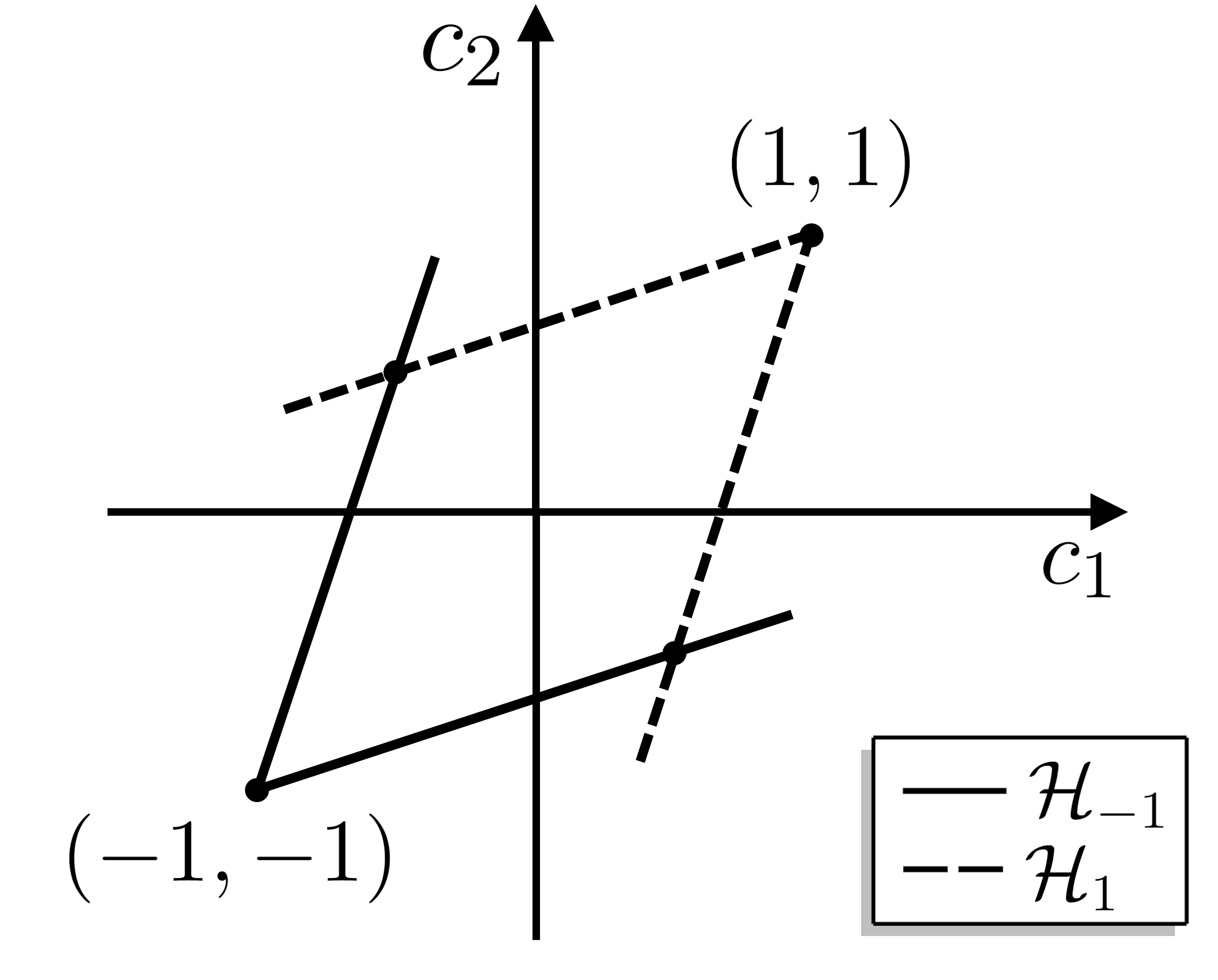
Proposition 1.

The following two-dimensional manifolds are invariant:

$$I_{1} =\{(a,r,s)\in\mathbb{R}^{3}:\;r>0\;\text{ and }\;s=2r\};$$

$$I_{2} =\{(a,r,s)\in\mathbb{R}^{3}:\;r>0\;\text{ and }\;s=-r\};$$

$$I_{3} =\{(a,r,s)\in\mathbb{R}^{3}:\;r<0\;\text{ and }\;s=r\};$$

$$I_{4} =\{(a,r,s)\in\mathbb{R}^{3}:\;r<0\;\text{ and }\;s=-2r\}.$$

By uniqueness of solutions, the following regions are also invariant:

$$R_{1} =\{(a,r,s)\in\mathbb{R}^{3}:s\geq-2r\;\text{ and }\;s\geq 2r\};$$

$$R_{2} =\{(a,r,s)\in\mathbb{R}^{3}:\;s\leq 2r\;\text{ and }\;s\geq-r\};$$

$$R_{3} =\{(a,r,s)\in\mathbb{R}^{3}:\;s\leq-r\;\text{ and }\;s\leq r\};$$

$$R_{4} =\{(a,r,s)\in\mathbb{R}^{3}:\;s\geq r\;\text{ and }\;s\leq-2r\}.$$

In what follows we will show that heteroclinic trajectories corresponding to traveling waves belong to the invariant manifolds $I_{1}$–$I_{4}$ (see Theorem 3 below).

3.1.3 Heteroclinic trajectories

We are looking for all values of $a_{0},b_{0},v\in\mathbb{R}$ such that there exist a heteroclinic trajectory $(a(\xi),b(\xi),r(\xi),s(\xi))$ of the dynamical system (20) that connects either a pair of critical points

$$(a,b,r,s)(-\infty)=(a_{0},b_{0},0,0)\quad\text{and}\quad(a,b,r,s)(+\infty)=(0,2,0,0),$$ (26)

or points

$$(a,b,r,s)(-\infty)=(0,-2,0,0)\quad\text{and}\quad(a,b,r,s)(+\infty)=(a_{0},b_{0},0,0).$$ (27)

An important step in proving Theorem 2 is the following Theorem 3, that gives an explicit relation between the fixed points for which there exist heteroclinic trajectories for the traveling wave dynamical system (20).

Theorem 3.

The following statements are valid:

Item 1. For any $v>0$ there exist exactly two values of the pair $(a_{0},b_{0})$ such that there exists a heteroclinic trajectory of the system (20), satisfying (26). Namely, either $(a_{0},b_{0})=(4v,-8v+2)$ or $(a_{0},b_{0})=(-4v,-8v+2)$. Also for any $v>0$ there does not exist any heteroclinic trajectory of the system (20), satisfying (27).

Item 2. For $v=0$ the system (20) does not have a heteroclinic trajectory that satisfies either $(a,b,r,s)(-\infty)=(0,b_{0},0,0)$ or $(a,b,r,s)(+\infty)=(0,b_{0},0,0)$ for any $b_{0}\in\mathbb{R}$.

Item 3. For any $v<0$ there exist exactly two values of the pair $(a_{0},b_{0})$ such that there exists a heteroclinic trajectory of the system (20), satisfying (27). Namely, either $(a_{0},b_{0})=(4v,-8v-2)$ or $(a_{0},b_{0})=(-4v,-8v-2)$. Also for any $v<0$ there does not exist any heteroclinic trajectory of the system (20), satisfying (26).

We postpone the proof of Theorem 3 to the Section 3.2, and first show how to prove Theorem 2 using Theorem 3. Indeed, by Theorem 3, we obtain in the original variables $c_{1}=(a+b)/2$, $c_{2}=(b-a)/2$:

• for every $v<0$ there exist exactly one traveling wave solution $c_{1,2}$ connecting $\sigma_{0}=(-1,-1)$ with each of the states

  $$\left[\begin{array}[]{ll}\sigma_{1}^{*}(v)=(c_{1}^{*}(v),c_{2}^{*}(v))=(-2v-1,-6v-1)\\ \sigma_{1}^{*}(v)=(c_{1}^{*}(v),c_{2}^{*}(v))=(-2v-1,-6v-1)\end{array}\right.$$

  Denote $\mathcal{H}_{-1}:=\{\sigma_{1}^{*}(v):v<0\}$, see Fig. 4.

• for every $v>0$ there exist exactly one traveling wave solution $c_{1,2}$ connecting each of the states

  $$\left[\begin{array}[]{ll}\sigma_{1}^{**}(v)=(c_{1}^{**}(v),c_{2}^{**}(v))=(-2v+1,-6v+1)\\ \sigma_{1}^{**}(v)=(c_{1}^{**}(v),c_{2}^{**}(v))=(-2v+1,-6v+1)\end{array}\right.$$

  with $\sigma_{2}=(1,1)$. Denote $\mathcal{H}_{1}:=\{\sigma_{1}^{**}(v):v>0\}$, see Fig. 4.

Notice that the intersection $\mathcal{H}_{1}\cap\mathcal{H}_{-1}$ consists of two points $(-\frac{1}{2},\frac{1}{2})$ and $(\frac{1}{2},-\frac{1}{2})$, and, thus, Theorem 2 is proven.

Figure 4: Representation of the sets $\mathcal{H}_{1}$ and $\mathcal{H}_{-1}$ in $(c_{1},c_{2})$-plane.

3.2 Proof of Theorem 3

Proof.

Item 1. First, we deal with the case $v>0$. The case $v<0$ can be managed similarly. Consider a trajectory $(a(\xi),b(\xi),r(\xi),s(\xi))$ of the system (20). Note that $(a(\xi),r(\xi),s(\xi))$ is a trajectory for the system (23).

We divide the proof of Theorem 3 for $v>0$ into smaller lemmas.

Lemma 2.

Let $(a,r,s)(-\infty)=(a_{0},0,0)$ for some $a_{0}\in\mathbb{R}$ and $(a(\xi),r(\xi),s(\xi))\not\equiv(a_{0},0,0)$. Then $|a_{0}|\geq\frac{4}{5}v$. In particular, there exists $\xi_{0}\in\mathbb{R}$ such that $a(\xi)$ is of constant sign for all $\xi<\xi_{0}$.

Proof.

Indeed,

$$\partial_{\xi}(r^{2}+s^{2})=2r\partial_{\xi}r+2s\partial_{\xi}s=2r\left(-vr-\frac{sa}{2}+\frac{a|r|}{2}\right)+2s(-vs-ra).$$

Estimating $rs\leq(r^{2}+s^{2})/2$ and $r|r|\leq(r^{2}+s^{2})$, we get

$$\partial_{\xi}(r^{2}+s^{2})\leq(r^{2}+s^{2})\left(-2v+\frac{5}{2}|a|\right).$$

By contradiction, if $|a_{0}|<\frac{4}{5}v$, then there exists $\xi_{0}\in\mathbb{R}$ such that $\partial_{\xi}(r^{2}+s^{2})\leq 0$ for all $\xi<\xi_{0}$. Taking into account that $r^{2}+s^{2}\to 0$ as $\xi\to-\infty$, we obtain $r^{2}+s^{2}\equiv 0$ for all $\xi<\xi_{0}$, and by uniqueness of solutions this holds for all $\xi\in\mathbb{R}$. ∎

Lemma 3.

There exists $\xi_{1}\in\mathbb{R}$ such that $r(\xi)$ is of constant sign for all $\xi<\xi_{1}$.

Proof.

As it is noticed in Proposition 1, the regions $R_{i}$, $i=1,2,3,4$, are invariant. If the trajectory $(a,r,s)\in R_{2}$ or $(a,r,s)\in R_{4}$, then the statement is obviously true.

Consider $(a,r,s)\in R_{1}$. By Lemma 2, for $\xi<\xi_{0}$ the sign of $a(\xi)$ is constant. Without loss of generality, assume that $a(\xi)>0$, $\xi<\xi_{0}$. Then

$$\partial_{\xi}r\biggr{\rvert}_{r=0}=-\frac{sa}{2}<0.$$

This implies that there exists $\xi_{1}\in\mathbb{R}$, $\xi_{1}<\xi_{0}$ such that $r(\xi)<0$ for $\xi<\xi_{1}$. The case $(a,r,s)\in R_{3}$ is similar. ∎

Lemma 4.

Let function $\alpha:\mathbb{R}^{3}\to\mathbb{R}$ satisfy

$$\frac{d}{d\xi}\alpha(x(\xi))=\alpha(x(\xi))\cdot\mu(x(\xi)),$$ (28)

where $\mu:\mathbb{R}^{3}\to\mathbb{R}$ is a continuous function. Assume that

$$\lim\limits_{\xi\to-\infty}x(\xi)=x^{-},\quad\mu(x^{-})<0,\quad\alpha(x^{-})=0,$$ (29)

then

$$\alpha(x(\xi))\equiv 0,\quad\xi\in\mathbb{R}.$$ (30)

Proof.

Let $\beta(\xi)=\alpha^{2}(x(\xi))$, then by (28)

$$\frac{d}{d\xi}\beta(\xi)=2\beta(\xi)\cdot\mu(x(\xi)).$$ (31)

Due to (29) and continuity of $\mu$, there exists $\xi_{0}\in\mathbb{R}$ such that for all $\xi<\xi_{0}$ the inequality $\mu(x(\xi))<0$ holds. Note that $\beta(\xi)\geq 0$ and, hence,

$$\frac{d}{d\xi}\beta(\xi)\leq 0,\quad\xi<\xi_{0}.$$

Thus, $\beta(\xi)$ is a nonincreasing nonnegative function on $(-\infty,\xi_{0})$. Since $\beta(\xi)\to 0$ as $\xi\to-\infty$ we conclude that $\beta(\xi)=0$ for $\xi<\xi_{0}$. Due to uniqueness of solution of (31), $\beta(\xi)\equiv 0$ for all $\xi\in\mathbb{R}$, which implies (30). ∎

Lemma 5.

Consider a trajectory $(a,r,s)$ of the system (23) such that
$(a,r,s)(-\infty)=(a_{0},0,0)$, $a_{0}\in\mathbb{R}$. Then $(a,r,s)\in I_{1}\cup I_{2}\cup I_{3}\cup I_{4}$, where $I_{k},k=1,2,3,4,$ are defined in Proposition 1.

Proof.

By Lemma 3, there exists $\xi_{1}\in\mathbb{R}$ such that $r(\xi)$ is of constant sign for all $\xi<\xi_{1}$.

Consider the case $r(\xi)>0$, $\xi<\xi_{1}$. By Lemma 2, we have $a(\xi)$ is of constant sign for $\xi<\xi_{1}$.

• If $a(\xi)>0$, $\xi<\xi_{1}$, then $-v-a/2<0$. Applying Lemma 4 to the relation (24) with $\alpha=r+s$, we obtain $r+s\equiv 0$, that is $(a,r,s)\in I_{2}$.

• If $a(\xi)<0$, $\xi<\xi_{1}$, then $-v+a<0$. Applying Lemma 4 to the relation (25) with $\alpha=2r-s$, we obtain $2r-s\equiv 0$, that is $(a,r,s)\in I_{1}$.

The case $r(\xi)<0$, $\xi<\xi_{1}$, is similar. ∎

So we reduced the problem to finding heteroclinic trajectories in each of the invariant half-planes $I_{k},k=1,2,3,4$.

Lemma 6.

• If $(a,r,s)\in I_{1}$, then there exist a unique $a_{0}\in\mathbb{R}$ such that there exists a heteroclinic trajectory, satisfying

  $$(a,r,s)(-\infty)=(a_{0},0,0)\quad\text{and}\quad(a,r,s)(+\infty)=(0,0,0).$$ (32)

  Moreover, $a_{0}=-4v$.

• If $(a,r,s)\in I_{4}$, then there exist a unique $a_{0}\in\mathbb{R}$ such that there exists a heteroclinic trajectory, satisfying (32). Moreover, $a_{0}=4v$.

• If $(a,r,s)\in I_{2}$ or $(a,r,s)\in I_{3}$, then there does not exist heteroclinic trajectories, satisfying (32).

Proof.

(i) The two-dimensional system inside $I_{1}$ takes the form:

$$\partial_{\xi}a =r,$$

$$\partial_{\xi}r =r\left(-v-\frac{a}{2}\right).$$

By a straightforward computation, we get

$$\frac{d}{d\xi}\left(r+\left(v+\frac{a}{2}\right)^{2}\right)=0.$$

This allows us to construct the phase portrait and write an explicit relation

$$r=-\left(v+\frac{a}{2}\right)^{2}+r_{0},\quad r_{0}\in\mathbb{R}.$$ (33)

Substituting it into the equation $\partial_{\xi}a=r$, it is clear, that there exists a unique $r_{0}$ and $a_{0}$ such that the trajectory $(a,r,s)$ lies in the region $\{r\geq 0\}$ and satisfies (32). Indeed, the condition $(a,r,s)(+\infty)=(0,0,0)$ implies $r_{0}=v^{2}$. The relation (33) immediately gives $a_{0}=-4v$.

(ii) The proof is similar to (i). The two-dimensional system inside $I_{4}$ takes the form:

$$\partial_{\xi}a =r,$$

$$\partial_{\xi}r =r\left(-v+\frac{a}{2}\right).$$

By a straightforward computation, we get that the following relation is valid on each trajectory

$$r=\left(-v+\frac{a}{2}\right)^{2}+r_{0},\quad r_{0}\in\mathbb{R}.$$ (34)

Substituting it into the equation $\partial_{\xi}a=r$, we obtain that there exists a unique $r_{0}$ and $a_{0}$ such that the trajectory $(a,r,s)$ lies in the region $\{r\leq 0\}$ and satisfies (32). Indeed, the condition $(a,r,s)(+\infty)=(0,0,0)$ implies $r_{0}=-v^{2}$. The relation (34) immediately gives $a_{0}=4v$.

(iii) The analogous reasoning for the half-planes $I_{2}$ and $I_{3}$ implies

$$\text{on }I_{2}: \quad\frac{d}{d\xi}\left(r-\frac{(a-v)^{2}}{2}\right)=0;\qquad \text{on }I_{3}:\quad\frac{d}{d\xi}\left(r+\frac{(a+v)^{2}}{2}\right)=0.$$

These relations allow to construct the phase portrait, and conclude that there are no heteroclinic trajectories in $I_{2}$ and $I_{3}$. ∎

Let us finish the proof of Theorem 3 for $v>0$. By Lemma 5, the heteroclinic trajectory $(a(\xi),r(\xi),s(\xi))$ necessarily lies in one of the four invariant half-planes $I_{k},k=1,2,3,4$. By Lemma 6, there exist exactly two heteroclinic trajectories inside $I_{k},k=1,2,3,4$ which satisfy (32).

In particular, if $(a,r,s)\in I_{1}$, then $s\equiv 2r$, thus, $\partial_{\xi}(b-2a)=0$. Taking into account (26), we obtain $b_{0}-2a_{0}=2$, which gives $b_{0}=-8v+2$.

If $(a,r,s)\in I_{4}$, then $s\equiv-2r$, thus, $\partial_{\xi}(b+2a)=0$. Taking into account (26), we obtain $b_{0}+2a_{0}=2$, which gives $b_{0}=-8v+2$.

This finishes the proof of Theorem 3 for $v>0$.

Item 2. Assume that there exists a heteroclinic trajectory $(a(\xi),r(\xi),s(\xi))$ connecting $(a_{0},0,0)$ and $(0,0,0)$. The first and the third equations of system (23) imply that

$$\frac{d}{d\xi}\left(s+\frac{a^{2}}{2}\right)=0,$$

and hence $s+\frac{a^{2}}{2}\equiv 0$. In particular, $a_{0}=0$ and the heteroclinic trajectory is actually homoclinic. Substituting $s=-a^{2}/2$ into (23), we get the following system

$$\begin{split}\partial_{\xi}a&=r,\\ \partial_{\xi}r&=\frac{a^{3}}{4}+\frac{a|r|}{2}.\end{split}$$ (35)

Analyzing the signs of $\partial_{\xi}a$ and $\partial_{\xi}r$ on lines $\{r=0\}$ and $\{a=0\}$, we conclude that the sets

$$A_{1}=\{r\geq 0,a\geq 0\},\quad A_{3}=\{r\leq 0,a\leq 0\}$$

are positive invariant and sets

$$A_{2}=\{r\leq 0,a\geq 0\},\quad A_{4}=\{r\geq 0,a\leq 0\}$$

are negative invariant, see Fig. 5.

Figure 5: Vector field (35) on axis $a=0$ and $r=0$.

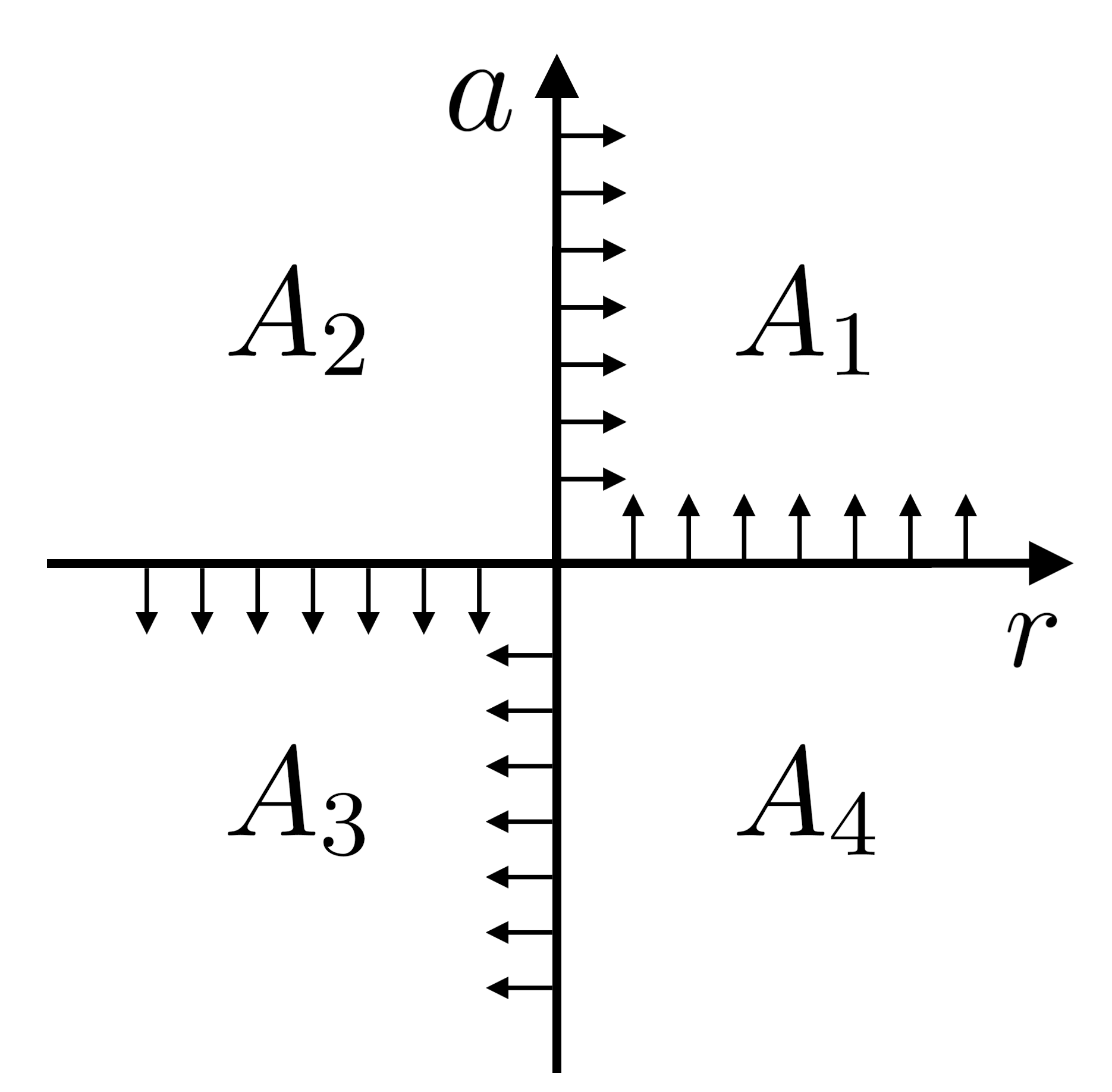
Note that in the sets $A_{1}$, $A_{3}$ the value of $a^{2}$ is monotonically increasing and in the sets $A_{2}$, $A_{4}$ the value of $r^{2}$ is monotonically decreasing. These statements contradict to the existence of nontrivial homoclinic trajectory associated to the point $(a=0,r=0)$.

Item 3. The case $v<0$ can be managed similarly to $v>0$. We omit the proof. ∎

3.3 Transversal intersection of stable and unstable manifolds

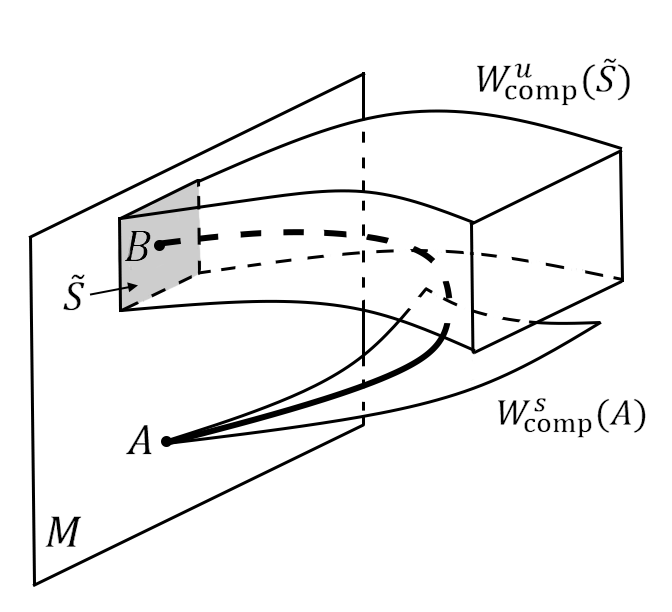
In this section we show that a heteroclinic trajectory, described in Theorem 3, can be seen as a transversal intersection of suitable stable and unstable manifolds. We will use this fact in Section 4 to prove the persistence of the heteroclinic trajectory under small perturbations.

We consider a system (20) under the constraint $r\leq 0$, that is

$$\begin{split}\partial_{\xi}a&=r,\\ \partial_{\xi}b&=s,\\ \partial_{\xi}r&=-vr-\frac{a}{2}(s+r),\\ \partial_{\xi}s&=-vs-ra.\end{split}$$ (36)

In what follows we assume $(a,b,r,s)\in\mathbb{R}^{4}$. We recall that $M$, defined in (22), is the set of fixed points of (36). By Theorem 3 Item 1, for $v>0$ there exists a heteroclinic trajectory between the fixed points:

$$A:=(a,b,r,s)(+\infty) =(0,2,0,0),\quad\text{and}\quad$$

$$B:=(a,b,r,s)(-\infty) =(4v,-8v+2,0,0),$$

such that $r(\xi)<0$, $\xi\in\mathbb{R}$. Fix $C$ to be any point on this trajectory (different from $A$ and $B$). Denote by $\phi_{\xi}(X)$ an image of the point $X\in\mathbb{R}^{4}$ under the flow of the system (36) at $\xi\in\mathbb{R}$. For any point $X\in\mathbb{R}^{4}$ we denote by $U_{X}$ some neighbourhood of $X$ in $\mathbb{R}^{4}$.

3.3.1 Stable manifold

First, notice that the tangent space at point $A$ has a splitting into stable and central parts:

$$\mathrm{T}_{A}\mathbb{R}^{4}=E^{s}(A)\oplus E^{c}(A),$$

where the central part $E^{c}(A)$ is spanned by eigenvectors corresponding to zero eigenvalues $\lambda_{3,4}=0$:

$$E^{c}(A)=\langle\begin{pmatrix}1&0&0&0\end{pmatrix}^{T},\begin{pmatrix}0&1&0&0\end{pmatrix}^{T}\rangle,$$

while the stable part $E^{s}(A)$ is spanned by eigenvectors corresponding to eigenvalues with negative real part $\lambda_{1,2}=-v$ (here $v>0$ by Theorem 3.1):

$$E^{s}(A)=\langle\begin{pmatrix}1&1&-v&-v\end{pmatrix}^{T},\begin{pmatrix}-1&2&v&-2v\end{pmatrix}^{T}\rangle.$$ (37)

By [20, Theorem 4.1(e)], there exists a local stable manifold $W^{s}_{loc}(A)$ defined by

$$W^{s}_{loc}(A)=\{X\in U_{A}:\phi_{\xi}(X)\to A\text{ as }\xi\to\infty\text{ and }\phi_{\xi}(X)\in U_{A}\text{ for all }\xi\geq 0\},$$ (38)

which is tangent to $E^{s}(A)$ at point $A$. Notice that $\mathrm{dim}(W^{s}_{loc}(A))=2$.

For the point $C$ on the trajectory there exists $\xi_{0}<0$ and $x\in W^{s}_{loc}(A)$ such that $C=\phi_{\xi_{0}}(x)$. Denote

$$W^{s}_{\mathrm{comp}}(A): =\{\phi_{\xi}(x)\in\mathbb{R}^{4}:\text{ for all }x\in W^{s}_{loc}(A),\xi\in[-\xi_{0}-1,0]\}.$$ (39)

Note that $C\in W^{s}_{\mathrm{comp}}(A)$.

In what follows we will need the following construction. Consider small enough $d>0$ and a set

$$A^{*}=\{(a,b,0,0),\mbox{ where }|a|,|b-2|<d\},$$ (40)

such that $\dim W^{s}_{loc}(x)=2$ for any $x\in A^{*}$.

3.3.2 Unstable manifold

The tangent space at point $B$ has a splitting into stable, central and unstable parts:

$$\mathrm{T}_{B}\mathbb{R}^{4}=E^{s}(B)\oplus E^{c}(B)\oplus E^{u}(B),$$

where the central part $E^{c}(B)$, analogously to the case for the point $A$, is spanned by eigenvectors corresponding to zero eigenvalues $\lambda_{3,4}=0$:

$$E^{c}(B)=\langle\begin{pmatrix}1&0&0&0\end{pmatrix}^{T},\begin{pmatrix}0&1&0&0\end{pmatrix}^{T}\rangle,$$

while the stable part $E^{s}(B)$ is spanned by eigenvector corresponding to eigenvalue with negative real part $\lambda_{1}=-5v$:

$$E^{s}(B)=\langle\begin{pmatrix}1&1&-5v&-5v\end{pmatrix}^{T}\rangle,$$

and the unstable part $E^{u}(B)$ is spanned by eigenvector corresponding to eigenvalue with positive real part $\lambda_{1}=v$:

$$E^{u}(B)=\langle\begin{pmatrix}-1&1&-v&2v\end{pmatrix}^{T}\rangle.$$ (41)

By [20, Theorem 4.1(be)], there exists a unique local unstable manifold $W^{u}_{loc}(B)$ defined by

$$W^{u}_{loc}(B)=\{X\in U_{B}:\phi_{\xi}(X)\to B\text{ as }\xi\to-\infty\text{ and }\phi_{\xi}(X)\in U_{B}\text{ for all }\xi\leq 0\},$$ (42)

which is tangent to $E^{u}(B)$ at point $B$. Notice that $\mathrm{dim}(W^{u}_{loc}(B))=1$.

Let $\tilde{S}$ be the neighbourhood of the point $B$ inside $M$:

$$\tilde{S}: =\{(a,b,0,0):a\in(3.9v,4.1v),b\in\bigl{(}0.9(-8v+2),1.1(-8v+2)\bigr{)}\}.$$ (43)

By [20, Theorem 4.1(ab)], there exists a unique local unstable manifold $W^{u}_{loc}(\tilde{S})$ which is tangent to $E^{u}(X)\oplus E^{c}(X)$ for any $X\in\tilde{S}$. Notice that $\mathrm{dim}(W^{u}_{loc}(\tilde{S}))=3$.

Due to Proposition 1, we observe that the set

$$\{s+2r=0\}:=\{(a,b,r,s):s+2r=0\}$$

is invariant and tangent to $E^{u}(X)\oplus E^{c}(X)$ for $X\in S$, thus $W^{u}_{loc}(\tilde{S})\subset\{s+2r=0\}$.

For the point $C$ on the trajectory there exists $\xi_{1}\geq 0$ and $y\in W^{u}_{loc}(\tilde{S})$ such that $C=\phi_{\xi_{1}}(y)$. Denote

$$W^{u}_{\mathrm{comp}}(\tilde{S}): =\{\phi_{\xi}(x)\in\mathbb{R}^{4}:\text{ for all }x\in W^{u}_{loc}(\tilde{S}),\xi\in[0,\xi_{1}+1]\}.$$ (44)

Note that $C\in W^{u}_{\mathrm{comp}}(\tilde{S})$.

Figure 6: Schematic representation of the transversal intersection of the stable manifold $W^{s}_{\mathrm{comp}}(A)$ and unstable manifold $W^{u}_{\mathrm{comp}}(\tilde{S})$.

3.3.3 Transversal intersection

The following Lemma claims that the manifolds $W^{s}_{\mathrm{comp}}(A)$ and $W^{u}_{\mathrm{comp}}(\tilde{S})$ intersect transversely in point $C$ (and, thus, in any point of the heteroclinic trajectory under consideration).

Lemma 7.

The manifolds $W^{s}_{\mathrm{comp}}(A)$ and $W^{u}_{\mathrm{comp}}(\tilde{S})$ intersect transversely in point $C$.

Proof.

Consider

$$W^{u}(\tilde{S}):=\{\phi_{\xi}(x)\in\mathbb{R}^{4}:\text{ for all }x\in W^{u}_{loc}(\tilde{S}),\xi\in[0,+\infty)\}.$$

It is clear that $A\in\mathrm{Cl}(W^{u}(\tilde{S}))$ and $W^{u}(\tilde{S})\subset\{s+2r=0\}$. Note that

$$T_{A}(\{s+2r=0\})+T_{A}(W_{loc}^{s}(A))=\mathbb{R}^{4}.$$

Hence, for any point $C^{*}=\phi_{\xi}(C)$ sufficiently close to $A$ (for some $\xi\in\mathbb{R}$), we obtain

$$T_{C^{*}}(W^{u}(\tilde{S}))+T_{C^{*}}(W_{loc}^{s}(A))=\mathbb{R}^{4}.$$

This implies that the intersection of the manifolds $W^{s}_{loc}(A)$ and $W^{u}(\tilde{S})$ is transversal in point $C^{*}$, hence the manifolds $W^{s}_{\mathrm{comp}}(A)$ and $W^{u}_{\mathrm{comp}}(\tilde{S})$ also intersect transversely in the point $C$ of the heteroclinic trajectory. ∎

Remark 6.

In Section 4 we restrict ourselves to considering the systems (36) for $v$ sufficiently close to $v_{1}^{*}$. In this case, instead of considering the sets $\tilde{S}$ depending on $v$ (see formula (43)), we define the unique set $S^{*}$ for all $v\in(v_{1}^{*}-\delta,v_{1}^{*}+\delta)$ for some small enough $\delta>0$:

$$S^{*}:=\{(a,b,0,0):a\in(3.9v^{*}_{1},4.1v^{*}_{1}),b\in\bigl{(}0.9(-8v^{*}_{1}+2),1.1(-8v^{*}_{1}+2)\bigr{)}\}.$$ (45)

By the same argument as before, the manifolds $W^{s}_{\mathrm{comp}}(A)$ and $W^{u}_{\mathrm{comp}}(S^{*})$ intersect transversally.

4 Proof of Theorem 1

First, in Section 4.1 we derive a dynamical system corresponding to traveling wave solutions for the two-tubes IPM equations (7)–(9), (13), (14). Also we formulate an auxiliary Theorem 4 on the existence of heteroclinic trajectories, and show how to derive Theorem 1 from Theorem 4. In Section 4.2 we present a proof of Theorem 4.

4.1 Traveling wave dynamical system

4.1.1 Derivation

We are looking for a traveling wave solution of the system (7)–(9), (13), (14) (for simplicity we denote the new unknown functions of one variable by the same notation $c_{1},\ldots$)

$$(c_{1},c_{2},u_{1},u_{2},q)(t,y)=(c_{1},c_{2},u_{1},u_{2},q)(\xi),\qquad\xi=y-vt,$$

connecting the states $(c_{1}^{-},c_{2}^{-},u_{1}^{-},u_{2}^{-},q^{-})$ and $(c_{1}^{+},c_{2}^{+},u_{1}^{+},u_{2}^{+},q^{+})$, i.e.

$$(c_{1},c_{2},u_{1},u_{2},q)(\pm\infty)=(c_{1}^{\pm},c_{2}^{\pm},u_{1}^{\pm},u_{2}^{\pm},q^{\pm}).$$

In variable $\xi$ the system (7)–(9), (13), (14) consists of the two equations (17)–(18) as before, and the additional ones:

$$\partial_{\xi}q =u_{1}-u_{2}+c_{1}-c_{2}, \partial_{\xi}u_{1} =q/l, \partial_{\xi}u_{2} =-q/l.$$ (46)

Using the unknown variables $(a,b,r,s)$, defined in formula (19), we write the system (17)–(18) and (46) in the form of a traveling wave dynamical system (47), as is stated in the following Lemma.

Lemma 8.

The traveling wave dynamical system for the two-tubes IPM equations (7)–(9), (13), (14) takes the following form $\mathrm{(}$in variables (19)$\mathrm{)}$:

$$\begin{split}\partial_{\xi}a&=r,\\ \partial_{\xi}b&=s,\\ \partial_{\xi}r&=-vr+u_{1}s+a\cdot\frac{|q|}{l},\\ \partial_{\xi}s&=-vs+u_{1}r+a\cdot\frac{q}{l},\\ \partial_{\xi}u_{1}&=\frac{q}{l},\\ \partial_{\xi}q&=2u_{1}+a.\end{split}$$ (47)

Proof.

As before it is clear that $\partial_{\xi}a=r$ and $\partial_{\xi}b=s$. Let’s show how to obtain the equation on $\partial_{\xi}s$. Summing up the equations (17)–(18), we get:

$$-v\partial_{\xi}(c_{1}+c_{2}) =-\partial_{\xi}(u_{1}c_{1}+u_{2}c_{2})+\partial_{\xi\xi}(c_{1}+c_{2}),$$

$$-v\partial_{\xi}(c_{1}+c_{2}) =-\partial_{\xi}u_{1}\cdot(c_{1}-c_{2})-u_{1}\cdot\partial_{\xi}(c_{1}-c_{2})+\partial_{\xi\xi}(c_{1}+c_{2}).$$

Using the relations (13) and (19), we get the necessary equation on $\partial_{\xi}s$.

Now let’s show how to obtain the equation on $\partial_{\xi}r$. Subtracting the equation (18) from (17), we get:

$$-v\partial_{\xi}(c_{1}-c_{2}) =-\partial_{\xi}(u_{1}c_{1}-u_{2}c_{2})+\partial_{\xi\xi}(c_{1}-c_{2})-2f,$$

$$-v\partial_{\xi}(c_{1}-c_{2}) =-\partial_{\xi}u_{1}\cdot(c_{1}+c_{2})-u_{1}\cdot\partial_{\xi}(c_{1}+c_{2})+\partial_{\xi\xi}(c_{1}-c_{2})-2f.$$

The sum $(-\partial_{\xi}u_{1}\cdot(c_{1}+c_{2})-2f)$ can be simplified:

$$-\partial_{\xi}u_{1}\cdot(c_{1}+c_{2})-2f =\begin{cases}-\partial_{\xi}u_{1}\cdot(c_{2}-c_{1}),&\partial_{\xi}u_{1}<0,\\ -\partial_{\xi}u_{1}\cdot(c_{1}-c_{2}),&\partial_{\xi}u_{1}\geq 0,\end{cases}=$$

$$=\begin{cases}\frac{aq}{l},&q<0,\\ -\frac{aq}{l},&q\geq 0,\end{cases}=-\frac{a|q|}{l}.$$

Substituting the new variables (19) into the equation (21), we get the necessary equation on $\partial_{\xi}r$. ∎

Assume $q\geq 0$. We rewrite the system (47) using the following change of variables:

$$r_{1}:=r-u_{1}a-\frac{a^{2}}{2},\qquad s_{1}:=s-u_{1}a-\frac{a^{2}}{2},\qquad q_{1}:=\frac{q}{\sqrt{l}},\qquad\varepsilon:=\sqrt{l}.$$

In new variables the system (47) becomes a slow-fast system in a standard form:

$$\begin{split}\partial_{\xi}a&=r_{1}+u_{1}a+\frac{a^{2}}{2},\\ \partial_{\xi}b&=s_{1}+u_{1}a+\frac{a^{2}}{2},\\ \partial_{\xi}r_{1}&=-v\left(r_{1}+u_{1}a+\frac{a^{2}}{2}\right)+u_{1}(s_{1}-r_{1})-a\left(r_{1}+u_{1}a+\frac{a^{2}}{2}\right),\\ \partial_{\xi}s_{1}&=-v\left(s_{1}+u_{1}a+\frac{a^{2}}{2}\right)-a\left(r_{1}+u_{1}a+\frac{a^{2}}{2}\right),\\ \varepsilon\cdot\partial_{\xi}u_{1}&=q_{1},\\ \varepsilon\cdot\partial_{\xi}q_{1}&=2u_{1}+a.\end{split}$$ (48)

If we formally consider $\varepsilon=0$ in (48), we get $u_{1}=-\frac{a}{2}=\frac{c_{2}-c_{1}}{2}$ and this expression coincides with the velocities in TFE model (16). Substituting this relation into the first four equations of the system (48), we obtain the traveling wave dynamical system for the TFE model (20) (note that formally we have $r_{1}=r$ and $s_{1}=s$) under the restriction $r\leq 0$.

Notice that the same reasoning for $q\leq 0$, leads to the traveling wave dynamical system for the TFE model (20) under the restriction $r\geq 0$.

This puts us into the framework of geometric singular perturbation theory (e.g. see the original work of Fenichel [17]), and determines our general strategy: knowing the existence of heteroclinic trajectory for the “unperturbed” system for $\varepsilon=0$ (two-tubes TFE equations), we prove that the heteroclinic trajectory persists under perturbation for small enough $\varepsilon>0$ (two-tubes IPM equations).

The set of fixed points for the system (48) for any $v\in\mathbb{R}$ and $\varepsilon>0$ coincides with the set

$$M:=\bigl{\{}(a,b,r_{1},s_{1},u_{1},q_{1})\in\mathbb{R}^{6}:r_{1}=s_{1}=q_{1}=0,u_{1}=-\frac{a}{2}\bigr{\}}.$$

4.1.2 Heteroclinic trajectories

We are looking for all values of $a_{0},b_{0},v\in\mathbb{R}$ such that there exist a heteroclinic trajectory $(a(\xi),b(\xi),r_{1}(\xi),s_{1}(\xi),u_{1}(\xi),q_{1}(\xi))$ of the dynamical system (48) that connects either a pair of critical points

$$\begin{split}(a,b,r_{1},s_{1},u_{1},q_{1})(-\infty)&=(a_{0},b_{0},0,0,-\frac{a_{0}}{2},0)\\ (a,b,r_{1},s_{1},u_{1},q_{1})(+\infty)&=(0,2,0,0,0,0),\end{split}$$ (49)

or points

$$\begin{split}(a,b,r_{1},s_{1},u_{1},q_{1})(-\infty)&=(0,-2,0,0,0,0)\\ (a,b,r_{1},s_{1},u_{1},q_{1})(+\infty)&=(a_{0},b_{0},0,0,-\frac{a_{0}}{2},0).\end{split}$$ (50)

An important step in proving Theorem 1 is the following Theorem 4, that provides a structure of the set of the fixed points for which there exist heteroclinic trajectories for the traveling wave dynamical system (48).

Theorem 4.

The following statements are valid:

Item 1. There exist $\varepsilon_{0},\delta>0$ such that for any $v\in(v_{1}^{*}-\delta,v_{1}^{*}+\delta)$ and for any $\varepsilon\in[0,\varepsilon_{0})$ there exists a pair $(a_{0},b_{0})=(a_{0}(v,\varepsilon),b_{0}(v,\varepsilon))$ such that there exists a heteroclinic trajectory of the system (48), satisfying (49). Moreover, we have:

• Continuous dependence: $a_{0}$ and $b_{0}$ depend continuously on $(v,\varepsilon)$ at any point $(v,\varepsilon)\in(v_{1}^{*}-\delta,v_{1}^{*}+\delta)\times[0,\varepsilon_{0})$.

• Consistency: $q_{1}(\xi)\geq 0$, $\xi\in\mathbb{R}$, on the heteroclinic trajectory.

Item 2. There exist $\varepsilon_{0},\delta>0$ such that for any $v\in(v_{2}^{*}-\delta,v_{2}^{*}+\delta)$ and for any $\varepsilon\in[0,\varepsilon_{0})$ there exists a pair $(a_{0},b_{0})=(a_{0}(v,\varepsilon),b_{0}(v,\varepsilon))$ such that there exists a heteroclinic trajectory of the system (48), satisfying (50). Moreover, we have:

• Continuous dependence: $a_{0}$ and $b_{0}$ depend continuously on $(v,\varepsilon)$ at any point $(v,\varepsilon)\in(v_{2}^{*}-\delta,v_{2}^{*}+\delta)\times[0,\varepsilon_{0})$.

• Consistency: $q_{1}(\xi)\geq 0$, $\xi\in\mathbb{R}$, on the heteroclinic trajectory.

Remark 7.

The analogue of Theorem 4 is also valid for the analogue of the system (48) if we assume $q_{1}\leq 0$ instead of $q_{1}\geq 0$.

Remark 8.

We do not claim uniqueness of heteroclinic solutions of (47) due to possibility of trajectories with not constant sign of $q$, which is not covered by our techniques. However, we expect that corresponding heteroclinic of (47) is unique.

We postpone the proof of Theorem 4 to the Section 4.2, and first show how to prove Theorem 1 using Theorem 4.

Note that for $\varepsilon=0$ the system (48) coincides with the system (20). This allows us to formally define $a_{0}(v,0)$ and $b_{0}(v,0)$ from Theorem 3. In particular, in the case $q_{1}\geq 0$ Theorem 4 Item 1 claims the continuous dependence of $a_{0}$ and $b_{0}$ at the point $(v,0)$, $v\in(v_{1}^{*}-\delta,v_{1}^{*}+\delta)$. This implies:

$$a_{0}(v,\varepsilon)=4v+g(v,\varepsilon),\qquad b_{0}(v,\varepsilon)=-8v+2+h(v,\varepsilon),$$

where $g(v,\varepsilon)$ and $h(v,\varepsilon)$ are continuous functions and $g(v,\varepsilon)$, $h(v,\varepsilon)\to 0$ as $\varepsilon\to 0$. Similar reasoning for the case $q_{1}\leq 0$ gives:

$$a_{0}(v,\varepsilon)=-4v+g_{1}(v,\varepsilon),\qquad b_{0}(v,\varepsilon)=-8v-2+h_{1}(v,\varepsilon),$$

where $g_{1}(v,\varepsilon)$ and $h_{1}(v,\varepsilon)$ are continuous functions; $g_{1}(v,\varepsilon)$, $h_{1}(v,\varepsilon)\to 0$ as $\varepsilon\to 0$.

By Theorem 4 we obtain in the original variables $c_{1}=(a+b)/2$, $c_{2}=(b-a)/2$, $l=\varepsilon^{2}$:

• there exists $l_{0}>0$ such that for all $l\in(0,l_{0})$ and all $v\in(v_{2}^{*}-\delta,v_{2}^{*}+\delta)$ there exists a traveling wave solution $(c_{1},c_{2},u_{1},u_{2},q)$ connecting $\sigma_{0}=(-1,-1,0,0,0)$ with the state $\sigma_{1}^{*}(v,l)=(c_{1}^{*}(v,l),c_{2}^{*}(v,l),u_{1}^{*}(v,l),u_{2}^{*}(v,l),q^{*}(v,l))$, where

  $$(c_{1}^{*}(v,l),c_{2}^{*}(v,l))=(-2v-1+z_{1}^{*}(v,l),-6v-1+z_{2}^{*}(v,l)),$$

  $$u_{1}^{*}(v,l)=-u_{2}^{*}(v,l)=(c_{2}^{*}(v,l)-c_{1}^{*}(v,l))/2,\qquad q^{*}(v,l)=0.$$ (51)

  Here $z_{1,2}^{*}(v,l)$ are continuous functions and $z_{1,2}^{*}(v,l)\to 0$ as $l\to 0$ for any fixed $v\in(v_{2}^{*}-\delta,v_{2}^{*}+\delta)$.

  Denote $\mathcal{H}_{-1}(l):=\{\sigma_{1}^{*}(v,l):v\in(v_{2}^{*}-\delta,v_{2}^{*}+\delta)\}$ and let $\Pi\mathcal{H}_{-1}(l)$ be the its projection of $\mathcal{H}_{-1}(l)$ on the plane $(c_{1},c_{2})$, see Fig. 7. Note that $\Pi\mathcal{H}_{-1}(0)$ coincides with the subset of $\mathcal{H}_{-1}$ (see Section 3.1.3) under the restriction $v\in(v_{2}^{*}-\delta,v_{2}^{*}+\delta)$.

• there exists $l_{0}>0$ such that for all $l\in(0,l_{0})$ and all $v\in(v_{1}^{*}-\delta,v_{1}^{*}+\delta)$ there exist a traveling wave solution $c_{1,2}$ connecting the state $\sigma_{1}^{**}(v,l)=(c_{1}^{**}(v,l),c_{2}^{**}(v,l),u_{1}^{**}(v,l),u_{2}^{**}(v,l),q^{**}(v,l))$ with the state $\sigma_{2}=(1,1,0,0,0)$, where

  $$(c_{1}^{**}(v,l),c_{2}^{**}(v,l))=(-2v+1+z_{1}^{**}(v,l),-6v+1+z_{2}^{**}(v,l)),$$

  $$u_{1}^{**}(v,l)=-u_{2}^{**}(v,l)=(c_{2}^{**}(v,l)-c_{1}^{**}(v,l))/2,\qquad q^{**}(v,l)=0.$$ (52)

  Here $z_{1,2}^{**}(v,l)$ are continuous functions and $z_{1,2}^{**}(v,l)\to 0$ as $l\to 0$ for any fixed $v\in(v_{1}^{*}-\delta,v_{1}^{*}+\delta)$.

  Denote $\mathcal{H}_{1}(l):=\{\sigma_{2}^{**}(v,l):v\in(v_{1}^{*}-\delta,v_{1}^{*}+\delta)\}$ and let $\Pi\mathcal{H}_{1}(l)$ be the projection of $\mathcal{H}_{1}(l)$ on the plane $(c_{1},c_{2})$, see Fig. 7. Note that $\Pi\mathcal{H}_{1}(0)$ coincides with the subset of $\mathcal{H}_{1}$ (see Section 3.1.3) under the restriction $v\in(v_{1}^{*}-\delta,v_{1}^{*}+\delta)$.

Figure 7: Representation of the sets $\Pi\mathcal{H}_{1}(l)$ and $\Pi\mathcal{H}_{-1}(l)$ in $(c_{1},c_{2})$-plane.

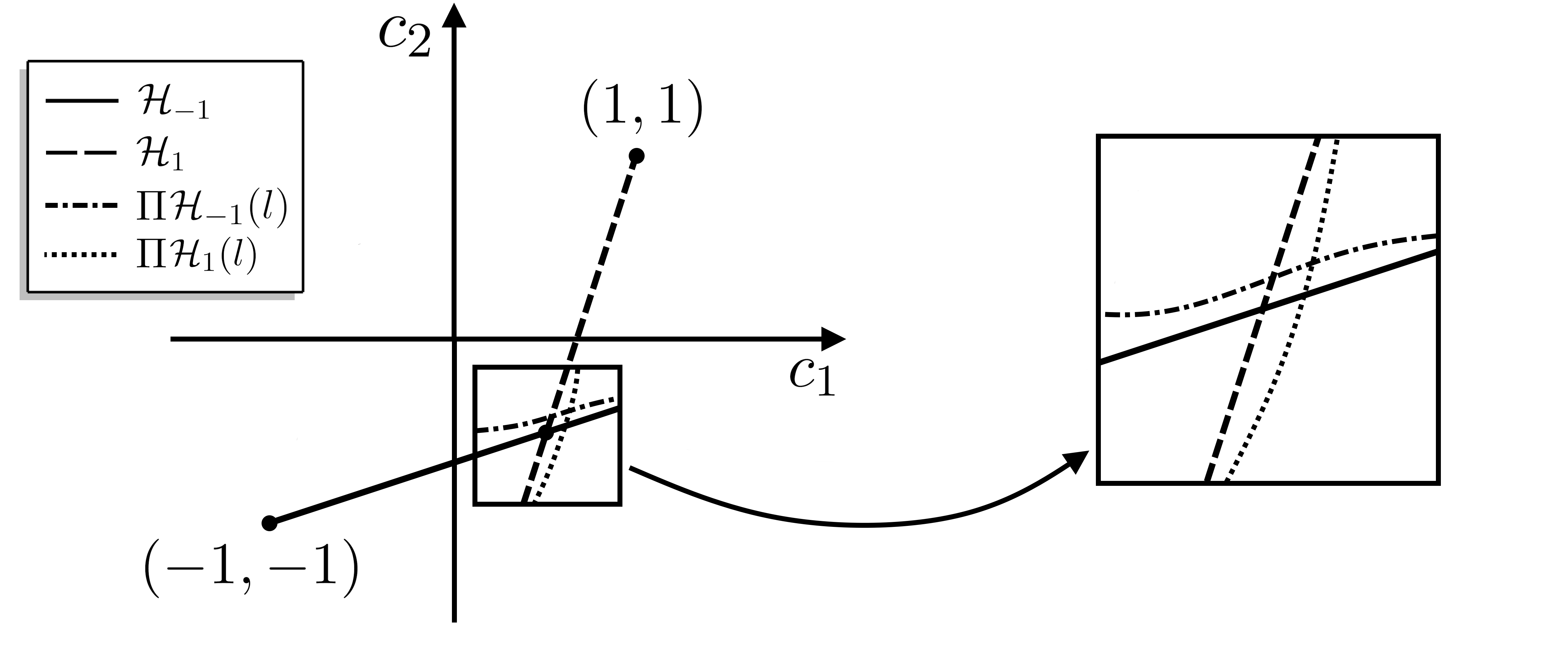
From Section 3.1.3 we know that the point $(1/2,-1/2)$ lies in the intersection of the curves $\Pi\mathcal{H}_{1}(0)$ and $\Pi\mathcal{H}_{-1}(0)$. For every fixed $l\geqslant 0$ the set $\Pi\mathcal{H}_{1}(l)$ (similarly, $\Pi\mathcal{H}_{-1}(l)$) is a curve and is close to $\Pi\mathcal{H}(0)$ and $\Pi\mathcal{H}_{-1}(0)$ near their intersection point. An easy topological argument shows that the curves $\Pi\mathcal{H}_{1}(l)$ and $\Pi\mathcal{H}_{-1}(l)$ have at least one point of intersection, that means there exist $v_{1}^{*}(l)$ and $v_{2}^{*}(l)$ such that the intersection $\Pi\mathcal{H}_{1}(l)\cap\Pi\mathcal{H}_{-1}(l)$ contains the point $(c_{1}^{*}(v_{2}^{*}(l),l),c_{2}^{*}(v_{2}^{*}(l),l))$ (or the same point $(c_{1}^{**}(v_{1}^{*}(l),l),c_{2}^{**}(v_{1}^{*}(l),l))$). Due to relations (51), (52), the curves $\mathcal{H}_{0}(l)$ and $\mathcal{H}_{1}(l)$ also intersect. By continuity argument, we obtain

$$\lim\limits_{l\to 0}c_{1}^{*}(v_{2}^{*}(l),l)=-1/2,\qquad\lim\limits_{l\to 0}c_{2}^{*}(v_{2}^{*}(l),l)=1/2,\qquad\lim\limits_{l\to 0}v_{1}^{*}(l)=-\lim\limits_{l\to 0}v_{2}^{*}(l)=1/4,$$

thus Theorem 1 is proven.

4.2 Proof of Theorem 4

We prove Theorem 4, Item 1, in four steps, following the scheme:

Step 1: we apply the geometric singular perturbation theory to the system (48), and reduce the problem to studying the heteroclinic trajectories in a 4-dimensional dynamical system (55), described in Lemma 9. Notice that this system (55) for $\varepsilon>0$ is a small perturbation of the dynamical system for TFE model ($\varepsilon=0$), studied in detail in Section 3.2.

Step 2: since the heteroclinic trajectory of the unperturbed system ($\varepsilon=0$) is a transverse intersection of some suitable stable and unstable manifolds (see Section 3.3), then it persists under small perturbation for $\varepsilon>0$. This guarantees the existence of a heteroclinic trajectory for (55), and thus, for (48) too.

Step 3: we prove the continuous dependence of the limiting points of the heteroclinic trajectory on the parameters $v$ and $\varepsilon$ (Item (a) of the Theorem 4).

Step 4: we prove that the found heteroclinic trajectory, indeed, satisfies the original assumption $q_{1}\geq 0$ (Item (b) of the Theorem 4).

The proof of Theorem 4, Item 2, is analogous to Item 1, so we omit it.

Step 1: application of geometric singular perturbation theory

In this section we apply the geometric singular perturbation theory (GSPT) for the system (48). This step allows to reduce the dimension of the dynamical system under consideration (from 6-dimensional to 4-dimensional). The original ideas on GSPT are due to N. Fenichel [17], the more recent advances on the theory can be found in books [24] and [46] (and references therein).

The system (48) has a structure of a “slow-fast” system (we denote $\partial_{\xi}$ by $\dot{\phantom{a}}$):

$$\begin{cases}\quad\dot{X}&=F(X,Y),\\ \varepsilon\cdot\dot{Y}&=AY-G(X),\end{cases}$$

where $X=\begin{pmatrix}a&b&r_{1}&s_{1}\end{pmatrix}^{T}\in\mathbb{R}^{4}$ and $Y=\begin{pmatrix}u_{1}&q_{1}\end{pmatrix}^{T}\in\mathbb{R}^{2}$, $A=\begin{pmatrix}0&1\\ 2&0\end{pmatrix}$; $F(X,Y)$ and $G(X)$ are the concrete vector functions. While in system (48) variable $v$ is a parameter, in this subsection it is convenient to include $v$ as a constant variable. Thus, we consider an extended system:

$$\begin{cases}\quad\dot{v}&=0,\\ \quad\dot{X}&=F(X,Y,v),\\ \varepsilon\cdot\dot{Y}&=AY-G(X).\end{cases}$$ (53)

System (53) is usually called “slow” system. For any $\varepsilon>0$ we obtain an equivalent “fast” system through the change of variables $\eta=\xi/\varepsilon$ (we denote $\partial_{\eta}$ by ^′):

$$\begin{cases}v^{\prime}&=0,\\ X^{\prime}&=\varepsilon\cdot F(X,Y,v),\\ Y^{\prime}&=\quad AY-G(X).\end{cases}$$ (54)

The set of fixed points of the fast system (54) for $\varepsilon=0$ is called a critical manifold. In our case for the fast-slow system (53)–(54) the critical manifold is:

$$K=\{(v,X,Y)\in\mathbb{R}^{7}:AY=G(X)\},\qquad\mathrm{codim}(K)=2.$$

The critical manifold $K$ is normally hyperbolic since the matrix of the first derivatives $D_{Y}(AY-G(X))\rvert_{K}=A$ has two eigenvalues $\lambda=\pm\sqrt{2}$ with non-zero real part.

Consider a compact submanifold $K_{0}\subset K$. Due to normal hyperbolicity of $K$, we can apply Fenichel’s result [17, Theorem 9.1]. Thus, there exists a manifold $K_{\varepsilon}\subset\mathbb{R}^{7}$ which is normally hyperbolic locally invariant under the flow of the system (53), diffeomorphic to $K_{0}$, and for some $H\in C^{1}$ the following inclusion is valid

$$K_{\varepsilon}\subset\{(v,X,Y)\subset\mathbb{R}^{7}:AY=G(X)+\varepsilon\cdot H(X,v,\varepsilon)\}.$$

As we will see below, in order to prove the existence of the heteroclinic trajectory, it is enough to restrict ourselves to the analysis of the dynamics inside the invariant manifold $K_{\varepsilon}$.

Lemma 9.

Let $(v(\xi),X(\xi),Y(\xi))\subset K_{\varepsilon}$ be a trajectory of (53), then there exists a function $F_{v,\varepsilon}:\mathbb{R}^{4}\to\mathbb{R}^{4}$ such that

1. $v(\xi)\equiv v^{*}$ for some $v^{*}\in\mathbb{R}$, and

   $$\dot{X}=F_{v^{*},\varepsilon}(X).$$ (55)

2. $F_{v,0}$ coincides with the right-hand side of (36).

Moreover, for $v$ close to $v_{1}^{*}$ and small enough $\varepsilon>0$ the following holds:

1. $F_{v,\varepsilon}(X)=0$ for $X\in A^{*}\cup S^{*}$, where $A^{*}$ is defined by (40), and $S^{*}$ is defined by (45).

2. $F_{v,\varepsilon}$ continuously depends on $(v,\varepsilon)$ in the $C^{1}_{loc}$-topology.

Proof.

Equality $v(\xi)\equiv v^{*}$ for some $v^{*}\in\mathbb{R}$ is a straightforward consequence of (53). Since $K_{\varepsilon}$ is invariant and determined by relation $AY=G(X)+\varepsilon\cdot H(X,v^{*},\varepsilon)$, we define

$$F_{v^{*},\varepsilon}(X):=F(X,A^{-1}(G(X)+\varepsilon H(X,v^{*},\varepsilon)),v^{*}),$$

which guarantees Item 1. Note that $F_{v,0}(X)=F(X,A^{-1}G(X),v)$ coincides with the right-hand side of (36), thus Item 2 is proved. Differentiability of $H$, $G$ and $F$ implies Item 4.

Consider a point $X=(a,b,0,0)\in A^{*}\cup S^{*}$, then point $(a,b,0,0,-a/2,0)$ is a fixed point of (48) for any $v,\varepsilon$. Note that for small $\varepsilon>0$ the point $(v,a,b,0,0,-a/2,0)$ lies in a small neighborhood of $K_{\varepsilon}$. Since $K_{\varepsilon}$ is invariant and normally hyperbolic, any trajectory staying in a small neighborhood of it actually belongs to it. Hence, $(v,a,b,0,0,-a/2,0)\in K_{\varepsilon}$, which concludes the proof of Item 3. ∎

Step 2: proof of the intersection of stable and unstable manifolds for perturbed system

Consider a small disc $\mathfrak{D}\in\mathbb{R}^{4}$ transversal to the vector field $F_{v_{1}^{*},0}$ at point $C\in W^{u}_{\mathrm{comp}}(S^{*})\cap W^{s}_{\mathrm{comp}}(A)$. Denote by $\phi_{\xi}^{v^{*},\varepsilon}(X)$ an image of the point $X\in\mathbb{R}^{4}$ under the flow of the system (55) at $\xi\in\mathbb{R}$, see Lemma 9.

Lemma 10.

For small enough $\varepsilon>0$ and $v$ close enough to $v_{1}^{*}$ there exists invariant manifolds $W^{u}_{loc,v,\varepsilon}(S^{*})$, $W^{u}_{\mathrm{comp},v,\varepsilon}(S^{*})$, $W^{s}_{loc,v,\varepsilon}(A)$, $W^{s}_{\mathrm{comp},v,\varepsilon}(A)$ of the flow $F_{v,\varepsilon}$ defined similarly to (42), (44), (38), (39). There exists point of intersection

$$C(v,\varepsilon)=W^{u}_{\mathrm{comp},v,\varepsilon}(S^{*})\cap W^{s}_{\mathrm{comp},v,\varepsilon}(A)\cap\mathfrak{D},$$

which depends continuously on $v,\varepsilon$ for $(v,\varepsilon)\in(v_{1}^{*}-\delta,v_{1}^{*}+\delta)\times[0,\varepsilon_{0})$ for some $\delta,\varepsilon_{0}>0$.

Proof.

The lemma is a straightforward consequence of the persistence of stable and unstable manifolds for normally hyperbolic sets [20, Theorem 4.1], Lemma 9 and transversality of the manifolds $W^{u}_{\mathrm{comp}}(S^{*})$ and $W^{s}_{\mathrm{comp}}(A)$. Below we provide a more detailed exposition.

Note that the set $S^{*}$ is normally hyperbolic for the flow $F_{v_{1}^{*},0}$. According to [20, Theorem 4.1(f)] for the flow $F_{v,\varepsilon}$ with $(v,\varepsilon)$ close to $(v_{1}^{*},0)$ there exists a unique locally invariant set $S^{*}_{v,\varepsilon}$ in a neighborhood of $S^{*}$ and its local unstable manifold $W^{u}_{loc,v,\varepsilon}(S^{*}_{v,\varepsilon})$ continuously depending on $v,\varepsilon$ in the $C^{1}$-topology. Due to Lemma 9 item 3, the set $S^{*}$ is invariant for $F_{v,\varepsilon}$, hence $S^{*}=S^{*}_{v,\varepsilon}$ and $W^{u}_{loc,v,\varepsilon}(S^{*}_{v,\varepsilon})=W^{u}_{loc,v,\varepsilon}(S^{*})$. Note that $W^{u}_{loc,v_{1}^{*},0}(S^{*})=W^{u}_{loc}(S^{*})$.

Similarly, the set $A^{*}$ is normally hyperbolic (attracting) for $F_{v_{1}^{*},0}$ and according to [20, Theorem 4.1(f)] and Lemma 9 Item 3, the stable manifold of $W^{s}_{loc,v,\varepsilon}(x)$ depends continuously on $v,\varepsilon$ in the $C^{1}$-topology for any $x\in A^{*}$. In particular, $W^{s}_{loc,v,\varepsilon}(A)$ depends continuously on $v,\varepsilon$ in the $C^{1}$-topology and $W^{s}_{loc,v_{1}^{*},0}(A)=W^{s}_{loc}(A)$.

Remark 9.

Note that [20, Theorem 4.1] is applicable to normally hyperbolic manifolds, while sets $S^{*}$, $A^{*}$ are topological discs. In order to be able to apply [20, Theorem 4.1], we suggest the following construction. Consider $U_{S^{*}}$ a neighborhood of $S^{*}$ (same as in definition of $W^{u}_{loc}(S^{*})$) and vector fields $F_{v_{1}^{*},0}^{*}$, $\tilde{F}_{v,\varepsilon}$ satisfying (we omit the construction)

• $F_{v_{1}^{*},0}^{*}(x)=F_{v_{1}^{*},0}(x)$, $\tilde{F}_{v,\varepsilon}(x)=F_{v,\varepsilon}(x)$ for $x\in U_{S^{*}}$,

• There are compact manifolds $N$, $N_{v,\varepsilon}$ normally hyperbolic for $\tilde{F}_{v_{1}^{*},0}$ and $\tilde{F}_{v,\varepsilon}$ respectively and $S^{*}\subset N$, $S^{*}\subset N_{v,\varepsilon}$.

• $\tilde{F}_{v,\varepsilon}$ is a small perturbation of $F_{v_{1}^{*},0}^{*}$.

Note that $W^{u}_{loc}(S^{*})$ and $W^{u}_{loc,v,\varepsilon}(S^{*})$ would be unstable manifolds of $S^{*}$ for vector fields $F_{v_{1}^{*},0}^{*}$, $\tilde{F}_{v,\varepsilon}$ as well and [20, Theorem 4.1] is applicable to the family of vector fields $\tilde{F}_{v,\varepsilon}$.

Similar construction is possible for the set $A^{*}$.

See also Theorem 4.5.1, Theorem 5.6.1 and Section 6.3 in [47].

Since $F_{v,\varepsilon}$ depends continuously on $v,\varepsilon$ in $C^{1}_{loc}$-topology, we see that the disk $\mathfrak{D}$ is transverse to the vector field $F_{v,\varepsilon}$ for $\varepsilon>0$ small enough and $v$ close to $v_{1}^{*}$. Similarly to (39) and (44), we define:

$$W^{s}_{\mathrm{comp},v,\varepsilon}(A): =\bigl{\{}\phi^{v,\varepsilon}_{\xi}(x)\in\mathbb{R}^{4}\,:\,\text{for all }x\in W^{s}_{loc,v,\varepsilon}(A),\,\xi\in[-\xi_{0}-1,0]\bigr{\}},$$

$$W^{u}_{\mathrm{comp},v,\varepsilon}(S^{*}): =\bigl{\{}\phi^{v,\varepsilon}_{\xi}(x)\in\mathbb{R}^{4}\,:\,\text{for all }x\in W^{u}_{loc,v,\varepsilon}(S^{*}),\,\xi\in[0,\xi_{1}+1]\bigr{\}}.$$

Continuous dependence of $W^{u}_{loc,v,\varepsilon}(S^{*})$ on $v,\varepsilon$ in the $C^{1}$-topology implies continuous dependence of $W^{u}_{\mathrm{comp},v,\varepsilon}(S^{*})$ on $v,\varepsilon$ in the $C^{1}$-topology. Similarly $W^{s}_{\mathrm{comp},v,\varepsilon}(A)$ depends continuously on $v,\varepsilon$ in the $C^{1}$-topology.

Transversality of intersection of the manifolds $W^{s}_{\mathrm{comp}}(A)=W^{s}_{\mathrm{comp},v_{1}^{*},0}(A)$ and $W^{u}_{\mathrm{comp}}(S^{*})=W^{u}_{\mathrm{comp},v_{1}^{*},0}(S^{*})$ implies that the set

$$\gamma_{v,\varepsilon}:=W^{u}_{\mathrm{comp},v,\varepsilon}(S^{*})\cap W^{s}_{\mathrm{comp},v,\varepsilon}(A)\neq\emptyset,$$

and depends continuously on $v,\varepsilon$ in $C^{1}$-topology. Note that $\dim\gamma_{v,\varepsilon}=1$ and $\gamma_{v,\varepsilon}$ is a trajectory of (55). Since $\mathfrak{D}$ is transverse to the vector field $F_{v,\varepsilon}$ and $\gamma_{v_{1}^{*},0}\cap\mathfrak{D}=C$ then $C(v,\varepsilon):=\gamma_{v,\varepsilon}\cap\mathfrak{D}$ depends continuously on $v,\varepsilon$. ∎

Step 3: Continuous dependence of intersection point

Let $D(v,\varepsilon):=\phi_{-\xi_{1}-1}^{v,\varepsilon}(C(v,\varepsilon))\in W^{u}_{loc,v,\varepsilon}(S^{*})$. Due to Lemma 10, the point $D(v,\varepsilon)$ depends continuously on $v$ and $\varepsilon$. For small enough $\varepsilon_{0}>0$ denote

$$\mathds{W}:=\{(v,\varepsilon,x):\;|v-v_{1}^{*}|<\varepsilon_{0},\;\varepsilon\in[0,\varepsilon_{0}),\;x\in W^{u}_{loc,v,\varepsilon}(S^{*})\}.$$

Consider the map

$$P:\mathds{W}\to S^{*},\quad\text{defined in such a way that }x\in W^{u}_{loc,v,\varepsilon}(P(v,\varepsilon,x)).$$

Continuous dependence of unstable lamination [20, Theorem 4.1(f)] implies that the map $P$ is uniquely defined and continuous. Hence, the point

$$B(v,\varepsilon):=P(v,\varepsilon,D(v,\varepsilon))$$

depends continuously on $v,\varepsilon$ and there exists a heteroclinic trajectory $X(\xi)$ of (55) that connects $B(v,\varepsilon)\in S^{*}$ and $A$. Hence, there exists a unique trajectory of (53), $(v,X(\xi),Y(\xi))\in K_{\varepsilon}$. Then $(X(\xi),Y(\xi))$ is a heteroclinic trajectory of (48) with given $(v,\varepsilon)$. As the point $B(v,\varepsilon)=(a_{0}(v,\varepsilon),b_{0}(v,\varepsilon),0,0)$ depends continuously on $v,\varepsilon$, so do the functions $a_{0}(v,\varepsilon)$, $b_{0}(v,\varepsilon)$.

Step 4: Consistency

First, we prove that the inequality $r_{1}\leq 0$ holds on heteroclinic trajectory $\Gamma_{v,\varepsilon}$, that connects $B(v,\varepsilon)$ and $A$. Consider $\widehat{\xi}>0$ such that

$$\phi_{-\widehat{\xi}}\,(C(v_{1}^{*},0))\in W^{u}_{loc}(B),\quad\phi_{\widehat{\xi}}\,(C(v_{1}^{*},0))\in W^{s}_{loc}(A).$$

Additionally, for $\varepsilon\in[0,\varepsilon_{0})$ for small enough $\varepsilon_{0}>0$ we can guarantee the inclusions

$$\phi_{-\widehat{\xi}}\,(C(v,\varepsilon))\in W^{u}_{loc,v,\varepsilon}(B(v,\varepsilon)),\quad\phi_{\widehat{\xi}}\,(C(v,\varepsilon))\in W^{s}_{loc,v,\varepsilon}(A).$$

We prove $r_{1}\leq 0$ at $\phi_{\xi}\,(C(v,\varepsilon))$ independently for $\xi<-\widehat{\xi}$,  $\xi\in[-\widehat{\xi},\widehat{\xi}]$ and $\xi>\widehat{\xi}$.

1. Consider $\xi<-\widehat{\xi}$. Note that the tangent vector at point $B$ to the manifold $W^{u}_{loc}(B)$ is (see (41))

   $$(-1,1,-v_{1}^{*},2v_{1}^{*})$$ (56)

   with non-zero $r_{1}$ component and heteroclinic trajectory $\Gamma_{v_{1}^{*},0}$ satisfies $r_{1}<0$, see (34). Hence, for small enough $\varepsilon_{0}>0$ the tangent vector to $W^{u}_{loc}(B(v,\varepsilon))$ at the point $B(v,\varepsilon)$ is close to (56). Thus, the inequality $r_{1}<0$ holds on $\Gamma_{v,\varepsilon}\cap W^{u}_{loc}(B(v,\varepsilon))$.

2. Consider $\xi\in[-\widehat{\xi},\widehat{\xi}]$. Note that interval $\xi\in[-\widehat{\xi},\widehat{\xi}]$ is bounded and for the set $\{\phi_{\xi}(C(v_{1}^{*},0)),\;\xi\in[-\widehat{\xi},\widehat{\xi}]\}$ the inequality $r_{1}<r^{c}$ holds for some constant $r^{c}<0$. Additionally decreasing $\varepsilon_{0}$, we can conclude that the inequality $r_{1}<r^{c}/2<0$ holds also for the set $\{\phi^{v,\varepsilon}_{\xi}(C(v,\varepsilon)),\;\xi\in[-\widehat{\xi},\widehat{\xi}]\}.$

3. Consider $\xi>\widehat{\xi}$. Note that $T_{A}W^{s}_{loc}(A)\subset\{r_{1}=-v_{1}^{*}a\}$, see (37). Hence, for sufficiently small $\varepsilon_{0}$ all points $(a,b,r_{1},s_{1})\in W^{s}_{loc,v,\varepsilon}(A)$ satisfy $r_{1}\in(-\frac{3}{2}v_{1}^{*}a,-\frac{1}{2}v_{1}^{*}a)$. So we can write $r_{1}(\xi)=k(\xi)a(\xi)$, where $k(\xi)\in(-\frac{3}{2}v_{1}^{*},-\frac{1}{2}v_{1}^{*})$, on the heteroclinic trajectory $\Gamma_{v,\varepsilon}$. Thus, $r_{1}(\xi)$ has a different sign than $a(\xi)$ and

   $$\dot{a}=\left(k(\xi)+u_{1}+\frac{a}{2}\right)a,\quad\xi\geq\widehat{\xi}.$$

   This implies that $a(\xi)$ has the same sign for all $\xi\geq\widehat{\xi}$ and $r_{1}(\xi)$ has an opposite sign. Since $r_{1}(\widehat{\xi})<0$ then $r_{1}(\xi)\leq 0$ for $\xi>\widehat{\xi}.$

We proved that the inequality $r_{1}\leq 0$ holds on the heteroclinic trajectory $\Gamma_{v,\varepsilon}$. Now we can prove that $q_{1}\geq 0$ on $\Gamma_{v,\varepsilon}$ (by contradiction). Equations (48) imply

$$q_{1}=-\frac{1}{2}\varepsilon r_{1}-\frac{1}{4}\varepsilon^{2}a\dot{q}_{1}+\frac{1}{2}\varepsilon^{2}\ddot{q}_{1}.$$ (57)

Note that $q_{1}\to 0$ as $\xi\to\pm\infty$. If $\inf_{\xi}q_{1}(\xi)<0$, then there exists $\xi_{2}\in\mathbb{R}$ such that $q_{1}(\xi_{2})=\inf_{\xi}q_{1}(\xi)<0$. Equation (57) does hold for $\xi=\xi_{2}$. Since left hand side of (57) is negative at $\xi=\xi_{2}$, and the right hand side of (57) is non-negative

$$-\frac{1}{2}\varepsilon r_{1}(\xi_{2})\geq 0,\quad\dot{q}_{1}(\xi_{2})=0,\quad\ddot{q}_{1}(\xi_{2})\geq 0,$$

we get a contradiction. Hence, $\inf_{\xi}q_{1}(\xi)\geq 0$, and Item (1b) of Theorem 4 is proved.

5 Discussions and generalizations

There are several directions for further investigation:

1.  Stability properties of the propagating terraces. Note that Theorem 1 establishes the existence of the propagating terrace consisting of two traveling waves for small values of parameter $l$. Nevertheless, numerical simulations show that for a typical initial data, the solution of (7)–(12) converges to a propagating terrace for any value of $l>0$. This observation suggests that a statement of Theorem 1 holds for any $l>0$, moreover, this propagating terrace is stable. At the same time, for system (7)–(12) it is possible to construct other solutions in a form of a propagating terrace consisting of $k$ traveling waves for any $k>2$, but we expect them to be unstable to small perturbations. Stability of propagation terraces for systems (7)–(12) is an open question.

2.   $n$-tubes model for gravitational fingering. It is possible to construct a model on similar principles for $n>2$ tubes. In that case for typical initial data, the solution converges to a propagating terrace consisting of several traveling waves. However, for $n>2$ limiting solution profile is not unique and usually consists of $k\geq n$ traveling waves. We discuss details of the construction and its properties in a separate paper [14].

3.  Two- and $n$-tubes model for viscous fingering. There is a natural analogue of a two-tubes model for the system (1), (2), (5) that describes viscous fingering phenomenon. Numerical simulations show that for typical initial data solution of a two-tubes model converges to a propagating terrace of two traveling waves. This observation suggests that analogue of Theorem 1 for the case of viscous fingers should be correct. Most of the steps of the proof of Theorem 1 could be repeated in that case. However, we cannot prove the existence of analogues of invariant hyperplanes $I_{1},I_{4}$. At the same time numerics shows that corresponding dynamical system has invariant sets which play a similar role. Detailed analysis of 2- and $n$-tube model for viscous liquids displacement is a subject for future research.

References

- [1] P. Bai, J. Li, F. R. Brushett, M. Z. Bazant, 2016. Transition of lithium growth mechanisms in liquid electrolytes, Energy & Environmental Science, 9, pp.3221–3229.
- [2] F. Bakharev, L. Campoli, A. Enin, S. Matveenko, Y. Petrova, S. Tikhomirov, A. Yakovlev, 2020. Numerical investigation of viscous fingering phenomenon for raw field data. Transport in Porous Media, 132, pp.443–464.
- [3] F. Bakharev, A. Enin, S. Matveenko, N. Rastegaev, D. Pavlov, S. Tikhomirov, 2023. Relation between size of mixing zone and intermediate concentration in miscible displacement. arXiv:2310.14260.
- [4] F. Bakharev, A. Enin, K. Kalinin, Yu. Petrova, N. Rastegaev, S. Tikhomirov, 2023. Optimal polymer slugs injection profiles. Journal of Computational and Applied Mathematics, 425, Paper No. 115042.
- [5] F. Bakharev, A. Enin, A. Groman, A. Kalyuzhnyuk, S. Matveenko, Yu. Petrova, I. Starkov, S. Tikhomirov, 2022. Velocity of viscous fingers in miscible displacement: comparison with analytical models. Journal of Computational and Applied Mathematics, 402, 113808.
- [6] E. Ben-Jacob, I. Cohen, H. Levine, 2000. Cooperative self-organization of microorganisms. Advances in Physics, 49, pp.395–554.
- [7] E. Ben-Jacob, N. Goldenfeld, B. Kotliar, J. Langer, 1984. Pattern selection in dendritic solidification. Physical Review Letters, 53, 2110.
- [8] R. Bianchini, T. Crin-Barat, M. Paicu, 2024. Relaxation approximation and asymptotic stability of stratified solutions to the IPM equation. Archive for Rational Mechanics and Analysis, 248(1), p.2.
- [9] A. Bose, 1995. Symmetric and antisymmetric pulses in parallel coupled nerve fibres. SIAM Journal on Applied Mathematics, 55(6), pp.1650–1674.
- [10] A. Castro, D. Córdoba and D. Lear, 2019. Global existence of quasi-stratified solutions for the confined IPM equation. Archive for Rational Mechanics and Analysis, 232, pp.437–471.
- [11] D. Córdoba, F. Gancedo, R. Orive, 2007. Analytical behavior of two-dimensional incompressible flow in porous media. Journal of Mathematical Physics, 48(6), 065206.
- [12] D. Cordoba, D. Faraco, F. Gancedo, 2011. Lack of uniqueness for weak solutions of the incompressible porous media equation. Archive for Rational Mechanics and Analysis, 200, pp.725–746.
- [13] A. Ducrot, T. Giletti, H. Matano, 2014. Existence and convergence to a propagating terrace in one-dimensional reaction-diffusion equations. Transactions of the American Mathematical Society, 366(10), pp.5541–5566.
- [14] Y. Efendiev, Y. Petrova, S. Tikhomirov Transversally Reduced Fingering Model (TRFM). In preparation.
- [15] T.M. Elgindi, 2017. On the asymptotic stability of stationary solutions of the inviscid incompressible porous medium equation. Archive for Rational Mechanics and Analysis, 225, pp.573–599.
- [16] R. Eymard, T. Gallouet and R. Herbin, 2000. Finite volume methods, in Handbook of numerical analysis, Vol. VII. North-Holland, Amsterdam, 713–1020.
- [17] N. Fenichel, 1979. Geometric singular perturbation theory for ordinary differential equations. Journal of Differential Equations, 31(1), pp.53–98.
- [18] C.H. Gao, 2011. Advances of Polymer Flood in Heavy Oil Recovery. SPE Heavy Oil Conference and Exhibition.
- [19] Th. Giletti, H. Matano, 2020. Existence and uniqueness of propagating terraces. Communications in Contemporary Mathematics 22.06, 1950055.
- [20] M.W. Hirsch, C.C. Pugh, M. Shub, 1970. Invariant manifolds. Bulletin of the American Mathematical Society, 76(5), pp.1015–1019.
- [21] H. Holden, N.H. Risebro, 2019. Models for dense multilane vehicular traffic. SIAM Journal on Mathematical Analysis, 51(5), pp.3694–3713.
- [22] G.M. Homsy, 1987. Viscous fingering in porous media. Annual Review of Fluid Mechanics, 19(1), pp.271–311.
- [23] A. Kiselev, Y. Yao, 2023. Small scale formations in the incompressible porous media equation. Archive for Rational Mechanics and Analysis, 247, p.1.
- [24] C. Kuehn, 2015. Multiple time scale dynamics (Vol. 191). Berlin: Springer.
- [25] L. W. Lake, R. Johns, B. Rossen, G. Pope, 2014. Fundamentals of Enhanced Oil Recovery, Society of Petroleum Engineers.
- [26] J. S. Langer, 1980. Instabilities and pattern formation in crystal growth. Reviews of modern physics, 52, p.1.
- [27] O. Manickam, G. M. Homsy, 1995. Fingering instabilities in vertical miscible displacement flows in porous media. Journal of Fluid Mechanics, 288, pp.75–102.
- [28] M. Matsushita, H. Fujikawa, 1990. Diffusion-limited growth in bacterial colony formation. Physica A: Statistical Mechanics and its Applications, 168, pp.498–506.
- [29] G. Menon, F. Otto, 2006. Diffusive slowdown in miscible viscous fingering. Communications in Mathematical Sciences 4.1, pp.267–273.
- [30] G. Menon, F. Otto, 2005. Dynamic scaling in miscible viscous fingering. Communications in Mathematical Physics, 257, pp.303–317.
- [31] J.C. Da Mota, S. Schecter, 2006. Combustion fronts in a porous medium with two layers. Journal of Dynamics and Differential Equations, 18(3), pp.615–665.
- [32] W.W. Mullins, R.F. Sekerka, 1963. Morphological stability of a particle growing by diffusion or heat flow. Journal of Applied Physics, 34, pp.323–329.
- [33] J.S. Nijjer, D.R. Hewitt, J.A. Neufeld, 2018. The dynamics of miscible viscous fingering from onset to shutdown. Journal of Fluid Mechanics, 837, pp.520–545.
- [34] D.W. Peaceman, H.H. Rachford, 1962. Numerical Calculation of Multidimensional Miscible Displacement. Society of Petroleum Engineers Journal, 2, 327–339.
- [35] M. Price, 2013. Introducing groundwater. Routledge.
- [36] P.G. Saffman, G.I. Taylor, 1958. The penetration of a fluid into a porous medium or Hele-Shaw cell containing a more viscous liquid. Proceedings of the Royal Society of London. Series A. Mathematical and Physical Sciences, 245(1242), pp.312-329.
- [37] G. Scovazzi, M.F. Wheeler, A. Mikelić, S. Lee, 2017. Analytical and variational numerical methods for unstable miscible displacement flows in porous media. Journal of Computational Physics, 335, pp.444-496.
- [38] J.J. Sheng, B. Leonhardt, N. Azri, 2015. Status of polymer-flooding technology, Journal of Canadian Petroleum Technology, 54(02), pp.116–126.
- [39] M.R. Soltanian, M. A. Amooie, N. Gershenzon, Z. Dai, R. Ritzi, F. Xiong, D. Cole, J. Moortgat, 2017. Environmental Science & Technology, 51(13), pp.7732–7741.
- [40] K. S. Sorbie, 1991. Polymer-Improved Oil Recovery. Springer Science & Business Media.
- [41] K.S. Sorbie, A.Y. Al Ghafri, A. Skauge, E. J. Mackay, 2020 On the modelling of immiscible viscous fingering in two-phase flow in porous media. Transport in Porous Media, 135, pp.331–359.
- [42] K.S. Sorbie, H.R. Zhang, N.B. Tsibuklis, 1995. Linear viscous fingering: new experimental results, direct simulation and the evaluation of averaged models. Chemical Engineering Science, 50(4), pp.601–616.
- [43] L. Székelyhidi Jr, 2012. Relaxation of the incompressible porous media equation. Annales scientifiques de l’Ecole normale supérieure, 45(3), pp.491–509.
- [44] S. Tikhomirov, F. Bakharev, A. Groman, A. Kalyuzhnyuk, Yu. Petrova, A. Enin, K. Kalinin, N. Rastegaev, 2021. Calculation of graded viscosity banks profile on the rear end of the polymer slug. SPE Russian Petroleum Technology Conference.
- [45] A.C. Vásquez, L.F. Lozano, W.S. Pereira, J.B. Cedro, G. Chapiro, , 2022. The traveling wavefront for foam flow in two-layer porous media. Computational Geosciences, 26(6), pp.1549–1561.
- [46] M. Wechselberger, 2020. Geometric singular perturbation theory beyond the standard form (Vol. 6). New York: Springer.
- [47] S. Wiggins, 2013. Normally hyperbolic invariant manifolds in dynamical systems, Applied Mathematical Sciences, Vol. 105, Springer New York, NY.
- [48] R.A. Wooding, 1969. Growth of fingers at an unstable diffusing interface in a porous medium or Hele-Shaw cell. Journal of Fluid Mechanics, 39(3), pp.477–495.
- [49] Y.C. Yortsos, D. Salin, 2006. On the selection principle for viscous fingering in porous media. Journal of Fluid Mechanics, 557, pp.225–236.
- [50] H.R. Zhang, K.S. Sorbie, N.B. Tsibuklis, 1997. Viscous fingering in five-spot experimental porous media: new experimental results and numerical simulation. Chemical Engineering Science, 52(1), pp.37–54.